Article

AI-Based Indoor Localization Using Virtual Anchors in Combination with Wake-Up Receiver Nodes

by
Sirine Chiboub
1,2,3,
Aziza Chabchoub
1,2,3,
Rihab Souissi
1,2,3,
Salwa Sahnoun
2,3,
Ahmed Fakhfakh
2,3 and
Faouzi Derbel
1,*
1
Smart Diagnostic and Online Monitoring, Leipzig University of Applied Sciences, Wächterstraße 13, 04107 Leipzig, Germany
2
Laboratory of Signals, Systems, Artificial Intelligence and Networks (SM@RTS), Digital Research Center of Sfax (CRNS), Sfax University, Sfax 3021, Tunisia
3
National School of Electronics and Telecommunications of Sfax, Technopole of Sfax, Sfax 3018, Tunisia
*
Author to whom correspondence should be addressed.
Electronics 2026, 15(3), 584; https://doi.org/10.3390/electronics15030584
Submission received: 22 December 2025 / Revised: 22 January 2026 / Accepted: 26 January 2026 / Published: 29 January 2026
(This article belongs to the Special Issue Advanced Indoor Localization Technologies: From Theory to Application)

Abstract

Accurate indoor localization is essential for navigation, monitoring, and industrial applications, especially in environments with Non-line of sight (NLOS) conditions. An indoor positioning system consists of fixed physical nodes, referred to as anchors, which serve as reference nodes with known locations, and entities that could be persons or objects that are also equipped with a node, referred to as targets, whose positions are estimated based on signal measurements exchanged with the surrounding anchors. Although RSSI is widely used due to hardware simplicity, its performance is often affected by signal degradation, multipath propagation, and environmental interference. To address this limitation, this work aims to develop an indoor positioning system, especially in wide areas with a minimal number of physical anchors, while maintaining high positioning accuracy and low latency. The proposed approach integrates VA, RSSI-based multilateration, and ML as a tool to refine and improve positioning accuracy, where ML models are used to predict the VA features and subsequently predict the corresponding distances. In addition, the system relies on energy-efficient WuRx nodes, which ensure a low power consumption and support on-demand communication. The study area covers two distinct floors with a total area of 366.9 m2, covered using only four physical anchors. Two studies were performed, the offline and the online, in order to evaluate the proposed system under both the theoretical performance and real implementation conditions. In the offline phase, hexagonal and rectangular grid architectures were compared using multiple machine learning models under varying numbers of virtual anchors. By comparing different architectures and machine learning models, the rectangular grid with 10 virtual anchors combined with the XGBoost model achieved the best performance, resulting in an RMSE of 1.49 m with a processing time of approximately 0.15 s . The online evaluation confirmed the performance of the proposed system, achieving an RMSE of 2.48 m .

1. Introduction

IPSs have emerged as a critical area of research due to their ability to provide accurate location data in environments where traditional satellite-based methods are ineffective, such as shopping centers and hospitals, where the tracking of objects and individuals is crucial [1]. GNSSs, such as the GPS, perform poorly indoors because satellite signals are attenuated, reflected by multiple paths, and obstructed by building structures, which leads to unreliable or unavailable position estimates [2].
To address these challenges, IPS technologies rely on signal measurements and positioning methods such as TOA [3], AOA [4], RSSI [5], and TDOA [6]. Localization techniques based on TOA, TDOA, and AOA generally require additional hardware and high-precision components, particularly for accurate time and angle measurements [7]. Such requirements often involve precise clock synchronization, high-resolution timing modules, specialized antenna arrays, or phase detection systems, which are used to extract angular information. These additional hardware components can significantly increase the complexity and cost of the system. This makes the initial deployment of these techniques in large-scale indoor environments potentially expensive and challenging compared with simpler approaches [8]. RSSI is one of the most widely employed methods in indoor positioning research due to its simplicity and low implementation cost. However, RSSI measurements exhibit significant variability in real indoor environments due to environmental factors such as multipath interference, shadowing, the movement of people or objects, and structural changes [9]. This complicates the estimation of reliable distances and further degrades the accuracy of localization in dynamic and mobile scenarios, where signal strength can fluctuate rapidly as the target moves [10]. Another significant challenge is achieving the network density required for accurate indoor positioning. In large-scale deployments, achieving high spatial resolution often requires a dense infrastructure of anchor nodes, which can substantially increase deployment complexity and cost [11]. The concept of virtual anchors has been proposed as a cost-effective alternative to address these limitations [12]. By using existing infrastructure or synthesized reference points, virtual anchors can reduce the number of physical devices needed while maintaining positioning performance. This can solve problems such as replacing anchors due to battery depletion and network costs [13]. Energy consumption in indoor localization applications is a significant challenge, particularly in systems requiring continuous or high-frequency communication and sensing. This can result in rapid battery depletion, leading to communication interruptions or the loss of target tracking [14].
In this paper, we propose a system that balances the reduction in network density and localization performance by introducing virtual anchors with the same characteristics as physical anchors. This system is supported by a carefully designed architecture that aims to minimize energy consumption while improving positioning accuracy. The system also employs nodes equipped with wake-up receivers for low-power energy consumption, combined with a dedicated communication protocol that activates only the nearest anchors when needed, with variation in the transmission power. To further enhance system accuracy, a machine learning-based approach is used for target tracking.
This paper is organized as follows. Section 2 reviews related works on indoor positioning systems. Section 3 describes the hardware system setup. Section 4 presents the system architecture and theoretical background. Section 5 introduces the proposed indoor localization approach. Section 6 reports the experimental results and offers a detailed discussion of the performance of the system. Finally, Section 7 concludes the paper and outlines potential directions for future research.

2. Related Works

Although the concept of VA has been explored for several years, it remains a highly promising approach for indoor localization and emerging smart environment applications. Its strength lies in dealing with the problems of deploying and maintaining physical anchors, which are often costly and logistically complex in dense or dynamic indoor settings. As a result, a growing number of recent studies continue to advance and refine the use of VA to enhance localization performance and scalability. Table 1 provides an insightful overview, summarizing the key performance characteristics of the technologies discussed in these studies.
The authors in [15] employ the UWB enhanced through an intelligent cluster-based VA selection algorithm. By strategically deploying 25 virtual anchors, this method achieves remarkable localization accuracy, with positioning errors lower than 0.8 m in open spaces and approximately 1.5 m in complex office environments. The optimized VA placement balances processing efficiency with precision, ensuring reliable tracking within a 6 m × 6 m area, even in dynamically changing indoor settings. In [16], the authors use RSSI-based multilateration, incorporating zone selection and virtual position-based adjustment methods within a ZigBee wireless sensor network (IEEE 802.15.4, 2.4 GHz). By employing a hybrid setup of four physical anchors and twelve virtual anchors (distributed as three per zone), this method significantly reduces the variability in RSSI signals, which often introduce challenges in indoor environments. Experimental results demonstrate that this approach achieves high localization accuracy, with an average error of 0.68 m in controlled laboratory settings ( 4 m × 4 m room), while maintaining an acceptable margin of 1.77 m in a larger corridor space ( 22 m × 9.3 m ). This represents a marked improvement of more than 57% compared to traditional multilateration approaches, highlighting its cost-effectiveness and reduced computational requirements.
The authors of [17] introduce an innovative indoor localization framework based on ANN and RSSI fingerprinting, introducing a smart virtual sensor paradigm. This system dynamically handles the failure of physical anchor nodes by employing ANN-based virtual sensors that rely on time series prediction to maintain continuous localization. Linear prediction is adopted as a simple baseline method, which uses the last known positions and assumes constant speed and straight line motion without any learning process. Experiments conducted in a 12.6 m × 4.5 m indoor environment show that the ANN significantly outperforms this baseline approach, achieving RMSE values of 0.27 m along the X-axis and 0.28 m along the Y-axis. Furthermore, the ANN model maintains high-precision predictions for up to 8 s, offering a robust and cost-effective solution that eliminates the need for additional hardware investments, making it a suitable option for scalable indoor localization applications.
In [18], the authors propose an indoor localization system that exploits UWB signals and multipath propagation to enable accurate positioning using a single physical anchor. Instead of deploying multiple anchors, the system treats signal reflections from surrounding walls as virtual anchor positions, which are obtained by mirroring the physical anchor position with respect to the room boundaries. By considering first-order reflections, a fixed number of virtual anchors associated with dominant reflective surfaces is obtained, thereby enhancing spatial diversity without increasing hardware complexity. The approach is experimentally validated in real indoor environments, including office and stockroom scenarios with areas of 31.6 m 2 and 46.7 m 2 , respectively. Experimental results demonstrate high localization accuracy, with 90% of positioning errors remaining below 0.20 m in office environments and 0.445 m in more cluttered spaces. In addition to localization accuracy, several studies emphasize other performance indicators, such as energy consumption, hardware cost, and model training complexity. ZigBee-based RSSI systems, illustrated in [19,20], generally offer low power operation but still require multiple physical anchors, which increases deployment and maintenance costs in large-scale environments. UWB-based solutions [21,22] achieve high positioning accuracy but rely on specialized and costly hardware, limiting their practical scalability. Fingerprinting-based ANN approaches [17] provide high localization precision in controlled scenarios, while they require extensive offline data collection and long training phases, which reduce adaptability in dynamic or multi-floor environments.
Recent studies have increasingly adopted virtual anchors as an effective strategy to enhance indoor positioning performance while reducing reliance on dense physical infrastructure. These works demonstrate the potential of virtual anchors to improve localization accuracy and system efficiency across indoor environments of different scales, including rooms, corridors, and open indoor spaces. Building on these advances, this paper aims to design and implement an innovative indoor positioning solution that employs virtual anchors to significantly reduce network density while extending coverage and maintaining high localization accuracy and low latency.

3. Hardware System Setup: Wake-Up Receiver Node

In this work, we employ a wireless sensor node architecture equipped with a wake-up receiver (WuRx), which enables continuous channel monitoring with minimal energy consumption. A WuRx is an RF receiver designed to provide continuous monitoring for a sensor node. By leveraging a combination of passive or active circuit techniques, the WuRx maintains extremely low power consumption, typically below 10 μW. The optimal WuRx design achieves an effective balance between idle listening power consumption and receiver sensitivity. The nodes employed in this work are based on the design presented in [23].
In listening mode, the WuRx attains a sensitivity of −61.6 dBm while consuming only   5.71 μ W . Upon detecting a WuPT containing its assigned address, it triggers an interrupt to the MCU, which subsequently transitions both the WuRx and the associated hardware components from sleep to active mode. The implemented hardware platform integrates a Texas Instruments MSP430G2553 microcontroller, selected for its support of Low Power Mode 4 (LPM4), in which the CPU and all peripheral modules are fully disabled, enabling an ultra-low current consumption of approximately 0.5 μ A . The primary radio transceiver exhibits a higher sensitivity of −107 dBm. Once a node receives a wake-up call, it responds with an acknowledgment. The addressing mechanism embedded in the wake-up packet ensures targeted activation and prevents unnecessary wake-ups, thereby maintaining energy efficiency. Figure 1 illustrates a communication system incorporating a wake-up from a sender node to a receiver node. The receiver uses an RF switch to alternate between the wake-up receiver and the main receiver [24]. This enables the main sensor node to remain in a low-power sleep mode until a designated trigger event occurs. These nodes are employed as target and anchor nodes within the proposed indoor localization system.

4. System Architecture and Theoretical Background

This section presents the overall system architecture and the theoretical background of the proposed indoor localization system, including RSSI-based multilateration, machine learning-based distance estimation, virtual anchor deployment, and the architecture of the proposed grid.

4.1. Received Signal Strength Indicator (RSSI)

RSSI is a commonly used measurement parameter in wireless networks that represents the received signal power at the receiver. In this work, RSSI values are collected from transmitting nodes and used as an input parameter for distance estimation. Although it generally decreases with increasing distance between the transmitter and receiver, this relationship is not strictly linear due to environmental effects such as electromagnetic noise, multipath propagation, and interference, which may cause signal fluctuations or unusually high values. It is expressed in dBm, ranging from about  0 dBm to around  −100 dBm. This makes RSSI a crucial parameter for optimizing network performance and ensuring reliable connectivity [25]. Environmental conditions, including temperature and humidity, can also affect RSSI stability [26]. Equations (1) and (2) present the path loss model of RSSI and the extracted distance [27].
RSSI ( d ) = RSSI ( d 0 ) 10 n log 10 d d 0 + X σ
d R S S I = 10 ( R S S I r e f R S S I ) 10 η
where d represents the distance between the transmitter and the receiver device, while d0 is the reference distance. The term RSSI(d0) denotes the RSSI value measured by the device at the reference distance d0. Additionally, Xσ refers to the Gaussian distributed noise with a mean of zero and a variance of σ2. The path loss exponent is denoted by η, which reflects environmental attenuation.

4.2. Multilateration

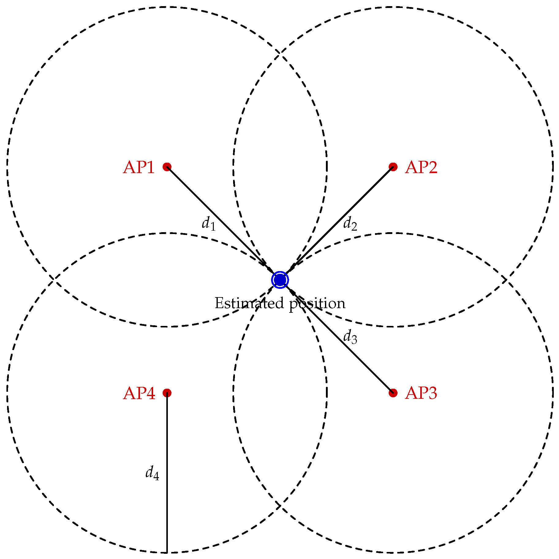
Multilateration is a positioning technique that determines the location of a target by using distance measurements from multiple reference nodes with known coordinates [28]. Trilateration is a fundamental case of multilateration for estimating positions, relying on distance measurements from three anchors with known coordinates. This method is widely employed due to its simplicity, accuracy, and low computational complexity, making it easy to implement on real embedded hardware platforms. In trilateration, the locations of fixed nodes and mobile targets are estimated using relative distance measurements. The target position is determined using the coordinates of reference nodes together with distance information derived from RSSI data, which reflects the distance between the target and each reference node [29].
d 1 = ( x x 1 ) 2 + ( y y 1 ) 2
d 2 = ( x x 2 ) 2 + ( y y 2 ) 2
d 3 = ( x x 3 ) 2 + ( y y 3 ) 2
d 4 = ( x x 4 ) 2 + ( y y 4 ) 2
where di is the distance between the target and each reference node.
d 1 2 d 2 2 = 2 x 1 x 2 y 1 y x 2 2 y 2 2 + 2 x 2 x + 2 y 2 y + x 1 2 + y 1 2
d 1 2 d 3 2 = 2 x 1 x 2 y 1 y x 3 2 y 3 2 + 2 x 3 x + 2 y 3 y + x 1 2 + y 1 2
d 1 2 d 4 2 = 2 x 1 x 2 y 1 y x 4 2 y 4 2 + 2 x 4 x + 2 y 4 y + x 1 2 + y 1 2
Equations (7)–(9) can be written in the system as follows:
d 1 2 d 2 2 + x 2 2 + y 2 2 x 1 2 y 1 2 d 1 2 d 3 2 + x 3 2 + y 3 2 x 1 2 y 1 2 d 1 2 d 4 2 + x 4 2 + y 4 2 x 1 2 y 1 2 = 2 ( x 2 x 1 ) 2 ( y 2 y 1 ) 2 ( x 3 x 1 ) 2 ( y 3 y 1 ) 2 ( x 4 x 1 ) 2 ( y 4 y 1 ) x y
As the number of reference nodes increases to N, the accuracy improves. Therefore, we extend the system of equations in (10) to include n equations, which allows the use of multilateration in position estimation [28]. This approach relies on distance measurements to four or more anchors with known coordinates (AP1–AP4), as schematically illustrated in Figure 2.
d 1 2 d 2 2 + x 2 2 + y 2 2 x 1 2 y 1 2 d 1 2 d 3 2 + x 3 2 + y 3 2 x 1 2 y 1 2 d 1 2 d 4 2 + x 4 2 + y 4 2 x 1 2 y 1 2 d 1 2 d n 2 + x n 2 + y n 2 x 1 2 y 1 2 = 2 ( x 2 x 1 ) 2 ( y 2 y 1 ) 2 ( x 3 x 1 ) 2 ( y 3 y 1 ) 2 ( x 4 x 1 ) 2 ( y 4 y 1 ) 2 ( x n x 1 ) 2 ( y n y 1 ) x y
Equation (11) can be written as the product of two matrices as follows (12):
B = A x y
where
B = d 1 2 d 2 2 + x 2 2 + y 2 2 x 1 2 y 1 2 d 1 2 d 3 2 + x 3 2 + y 3 2 x 1 2 y 1 2 d 1 2 d 4 2 + x 4 2 + y 4 2 x 1 2 y 1 2 d 1 2 d n 2 + x n 2 + y n 2 x 1 2 y 1 2
and A is
A = 2 ( x 2 x 1 ) 2 ( y 2 y 1 ) 2 ( x 3 x 1 ) 2 ( y 3 y 1 ) 2 ( x 4 x 1 ) 2 ( y 4 y 1 ) 2 ( x n x 1 ) 2 ( y n y 1 )
To calculate the solution of Equation (12), we derived Equation (15)
x y = ( A T A ) 1 A T B

4.3. Virtual Anchors

To reduce hardware costs, we propose the use of virtual anchors. Virtual anchors emulate real physical anchors without requiring actual hardware deployment. Unlike physical anchors, which are fixed devices installed in the environment, VAs exist only in the digital domain, and their features are generated by machine learning models based on signal measurements from real anchors and the associated virtual anchor positions. In our study, the integration of machine learning is motivated by the complex and highly nonlinear relationship between RSSI measurements and distance, particularly under NLOS conditions, where multipath propagation and environmental variability significantly affect signal behavior.
Machine learning models are able to capture these nonlinearities directly from data, enabling more robust estimation of virtual anchor features and the corresponding distances. Consequently, the proposed approach enhances localization accuracy and system scalability while reducing infrastructure density and deployment costs. For each virtual anchor, we define x and y coordinates according to a specific architecture, which will be described in the following section. Using these coordinates along with the parameters of the real anchors, a machine learning model predicts the corresponding features of each virtual anchor, including RSSI, temperature, and humidity. Each VA is also assigned a unique ID, creating a dataset that reflects the real anchor data but incorporates the additional virtual anchors. By integrating these predicted virtual anchors into the multilateration process, the effective number of reference points is increased without adding new hardware. This strategy significantly reduces the number of required real anchors, lowers deployment costs, and improves localization accuracy and coverage, particularly in NLOS indoor environments. Figure 3 illustrates the complete process of creating virtual anchors.

4.4. Machine Learning Algorithms

Machine learning algorithms play a key role in modern indoor localization systems by improving localization accuracy [30]. Machine learning is used in indoor localization to improve distance prediction accuracy, which is essential for multilateration-based positioning. In this work, machine learning models are first applied to predict the features of virtual anchors. Then, it is used to predict distances of real anchors. The selected machine learning algorithms are tree-based regression models. They are suitable for learning the RSSI-based path loss relationship and for capturing nonlinear effects under noisy measurement conditions. Accordingly, distance prediction is interpreted as the path loss model described in Equations (1) and (2). Random Forest represents bagging-based ensembles, which are known for their robustness to noise and stable performance [31]. XGBoost and CatBoost represent gradient boosting approaches, which are designed to achieve higher predictive accuracy by sequentially correcting model errors. Other tree-based methods were not included, as the selected algorithms already represent the main ensemble learning strategies relevant to the considered localization task, allowing the experimental framework to remain focused and manageable.

4.4.1. Random Forest Algorithm (RF)

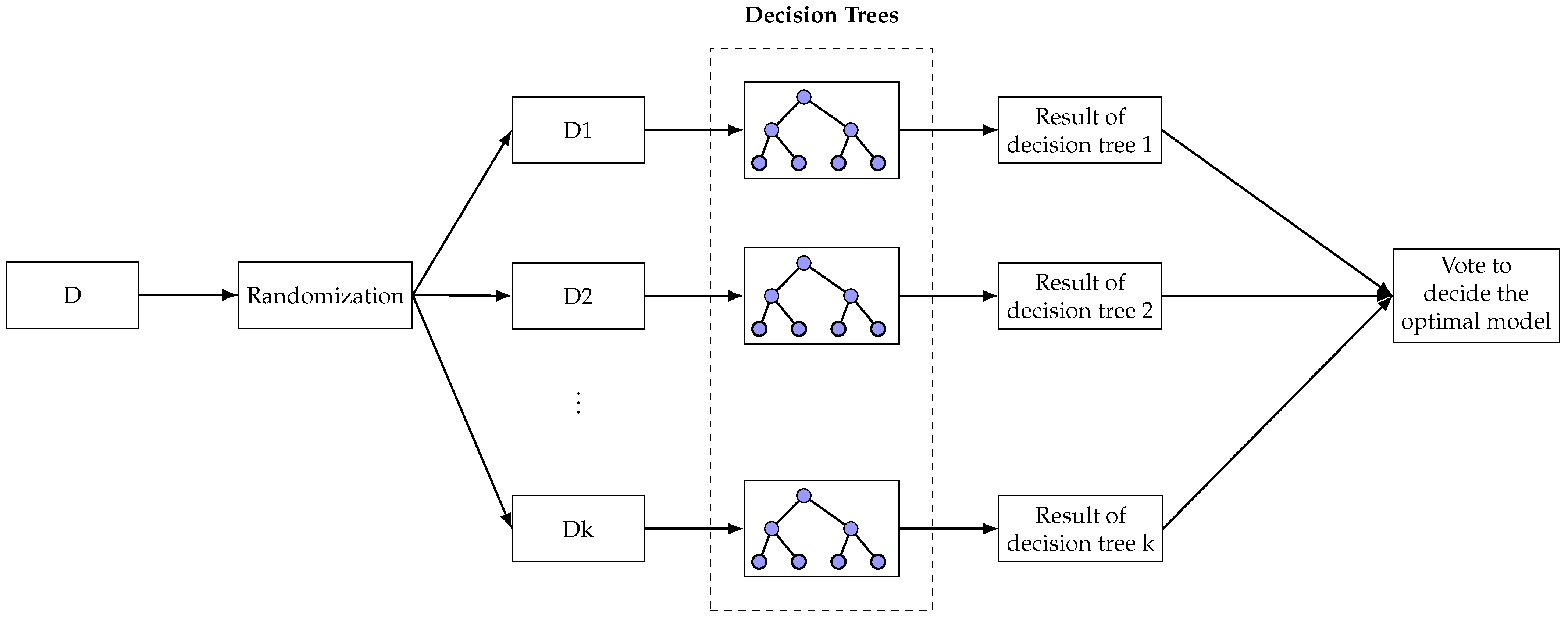
RF is an ensemble learning algorithm combining multiple decision trees to enhance predictive accuracy and avoid overfitting. It is robust, handles high-dimensional data effectively, and is widely used for classification and regression tasks.
RF combines multiple weak learners to create a robust model that reduces overfitting and minimizes individual errors, thereby improving accuracy and stability [32]. The performance of Random Forest is mainly influenced by key hyperparameters, including the number of iterations, which specifies the number of decision trees in the ensemble, and max depth, which controls the complexity of individual trees. Increasing the number of iterations generally leads to more stable predictions at the cost of higher computational complexity, while larger values of max depth enable the model to capture more complex patterns, but may increase the risk of overfitting [33]. Figure 4 illustrates the architecture of the RF algorithm. The model employs a bagging strategy, in which each decision tree is trained on a randomly resampled subset of the original dataset generated with replacement. The individual trees operate independently, and the final prediction is obtained by aggregating their outputs, using averaging for regression tasks or majority voting for classification.

4.4.2. CatBoost Algorithm

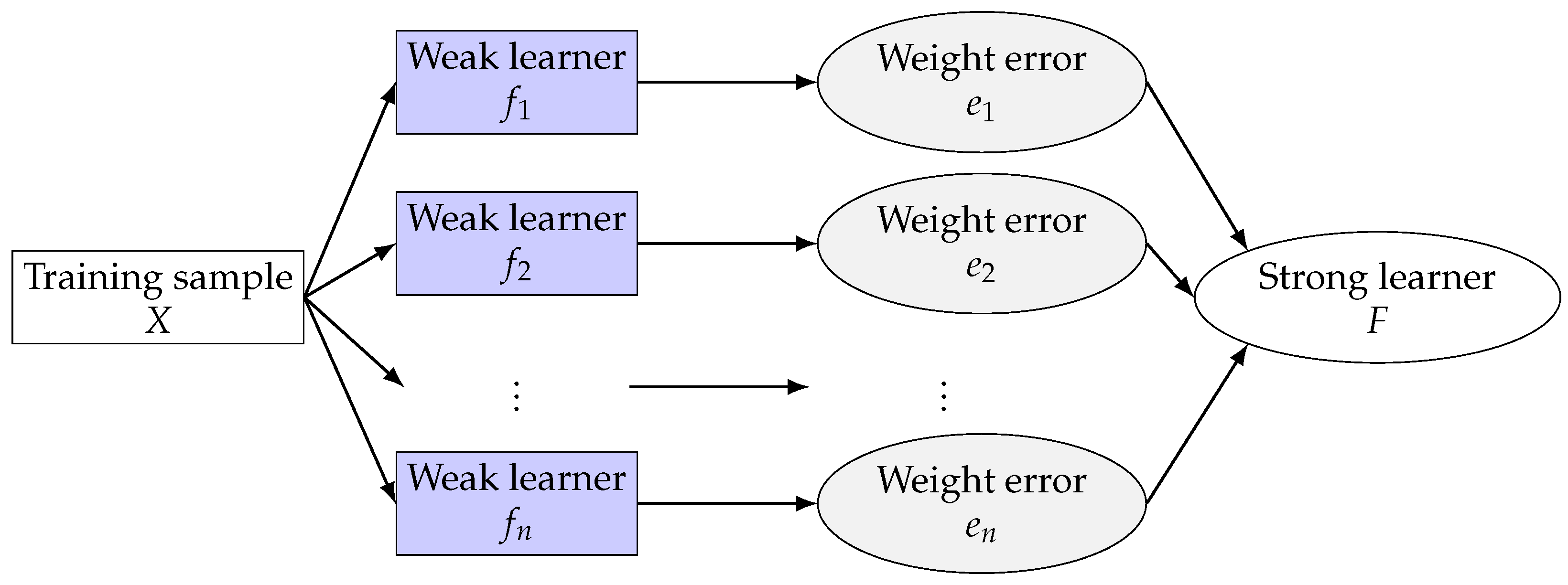
CatBoost is a gradient boosting method designed to improve the performance of decision tree ensembles, particularly when handling complex and heterogeneous feature spaces [34]. In addition to its robustness to categorical data, CatBoost is well suited for RSSI-based indoor localization due to its ability to effectively model nonlinear relationships and mitigate overfitting on noisy measurements. Unlike other boosting methods, it employs ordered boosting and advanced regularization techniques to reduce prediction bias and gradient distortion, leading to improved accuracy and generalization [35].
Figure 5 shows the general boosting principle used by CatBoost. The training data are processed sequentially by multiple weak learners (decision trees), where each new learner focuses on reducing the residual errors of the previous ones. The outputs of these weak learners are then combined to form a strong predictive model. In CatBoost-based regression models, the performance is strongly affected by the choice of several hyperparameters. In particular, the tree depth influences the ability of the model to capture complex patterns, the learning rate controls the speed and stability of the training process, and the number of iterations determines the overall model capacity. Adjusting these hyperparameters allows balancing prediction accuracy and overfitting, and their optimization has been shown to significantly improve regression performance in recent studies [36].

4.4.3. XGBoost Algorithm

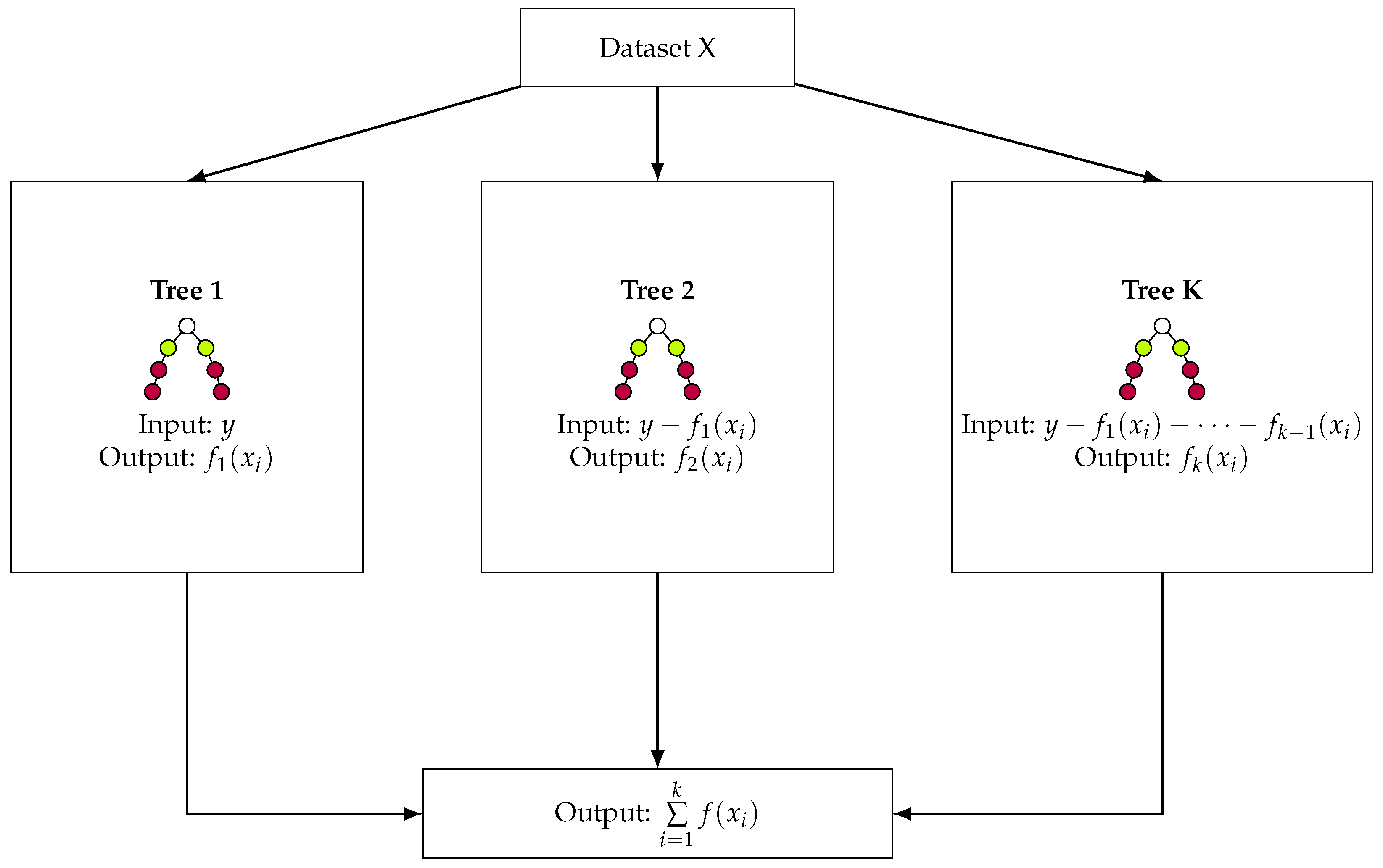
XGBoost is a scalable, efficient, open-source machine learning framework using gradient-boosted decision trees for classification, regression, and ranking tasks. It employs parallel processing, GPU acceleration, built-in L1 and L2 regularization, and automatically handles missing data, ensuring robust and accurate performance on large datasets [37]. The performance of XGBoost is highly dependent on several key hyperparameters, including max depth, which controls the complexity of individual trees, learning rate, which determines the contribution of each boosting iteration, and number of iterations, which specifies how many trees are sequentially added to the ensemble and affects the trade-off between accuracy and overfitting [38]. Figure 6 illustrates the overall structure of the XGBoost algorithm. The dataset X serves as the input to a sequence of boosted decision trees, where each tree is trained to minimize the residual errors produced by the preceding models. Tree 1 generates the initial prediction f1(xi), which is then used to compute the residuals for Tree 2. This iterative process continues until Tree K, with each subsequent tree refining the model by learning from the remaining errors. The final prediction is obtained by aggregating the outputs of all trees, expressed as k = 1 K f k ( x i ) , representing the ensemble output generated through gradient boosting.

4.5. Network Architecture and Deployment

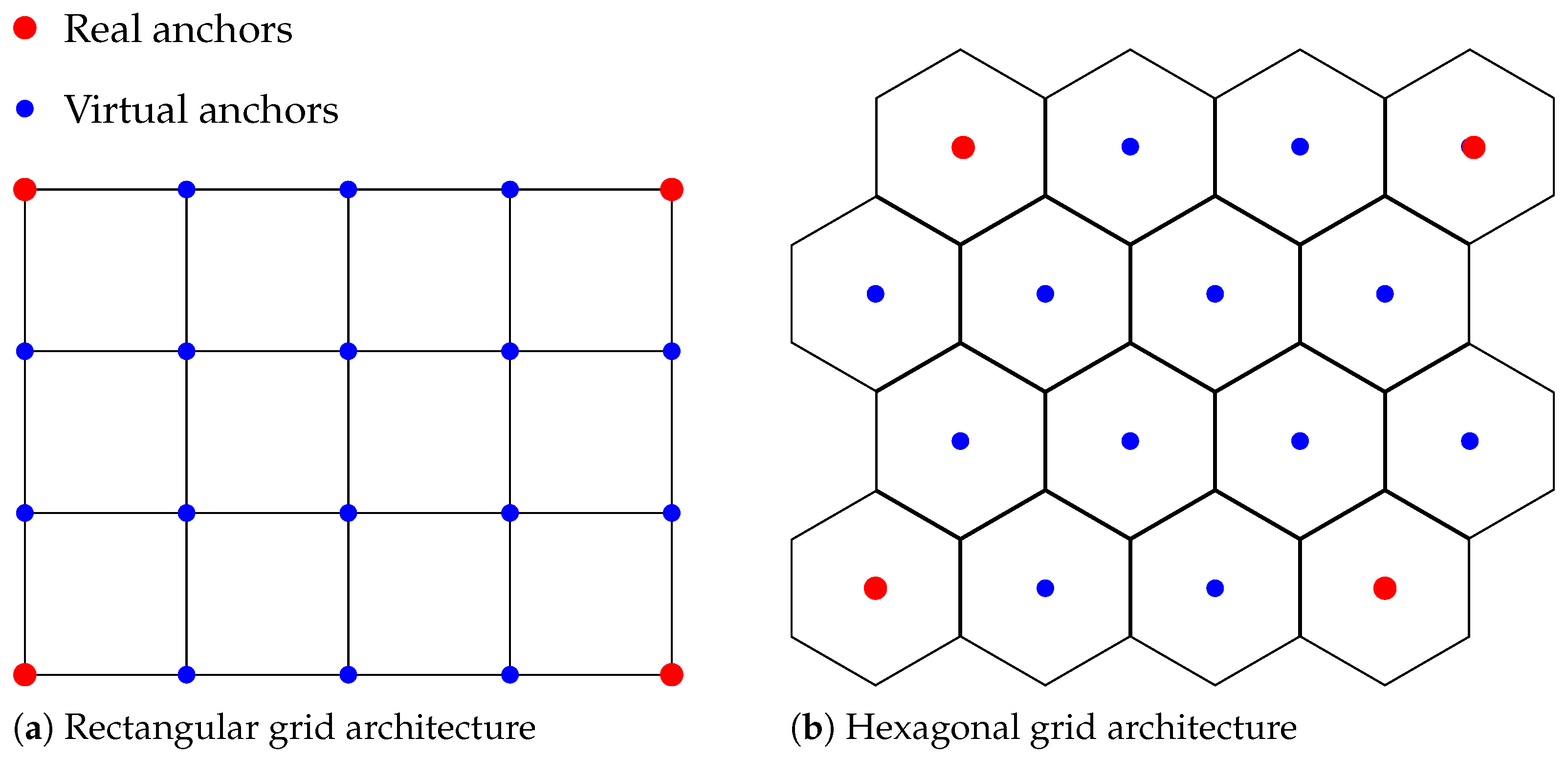
Efficient positioning of anchor nodes within a structured architecture plays a critical role in minimizing localization errors and reducing the impact of environmental interference [39]. The choice of the grid architecture directly affects the geometric distribution of reference nodes, which determines the quality of the distance intersections used in multilateration. A well-designed architecture improves geometric diversity, reduces position ambiguity, and enhances the robustness of localization results, particularly in indoor environments affected by RSSI noise and multipath propagation. In this study, as shown in Figure 7, two distinct grid configurations were explored, a rectangular grid and a hexagonal grid. The placement of virtual anchors is based on the study presented in [39].
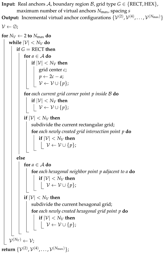
As demonstrated in the Algorithm 1, a structured placement strategy is adopted for each architecture to maximize coverage. The algorithm takes as inputs the set of real anchors A , the boundary region B defining the deployment area, the grid type G ∈ {RECT, HEX}, the maximum number of virtual anchors Nmax, and the grid spacing parameter s. Real anchors are positioned near the extremities of each area to provide reference boundaries, while VAs are placed according to the underlying grid segmentation, and their coordinates are generated using predefined geometric grid rules. The algorithm incrementally builds the virtual anchor set V , where NV represents the number of virtual anchors at each incremental step and is progressively increased from 2 to Nmax. In the rectangular architecture, VAs are added progressively following a rectangular grid. Initially, VAs are positioned symmetrically with respect to the real anchors to maintain geometric balance, using the grid center c and the symmetry rule p = 2ca for each real anchor a A . Following this, VAs are placed at the corners of the rectangular grid defined within the boundary region B . Additional anchors are generated by subdividing the grid according to the spacing parameter s, which increases spatial density while preserving uniform spacing. In the hexagonal grid, VAs are placed adjacent to the real anchors to form a hexagonal grid with uniform spacing s. For example, when two VAs are introduced, each hexagonal cell is centered between two real anchors and two VAs, preserving geometric symmetry within the boundary region B . As more VAs are introduced, the hexagonal grid is progressively subdivided based on coverage requirements, generating new grid points according to the spacing parameter s and increasing spatial density while maintaining the hexagonal structure.
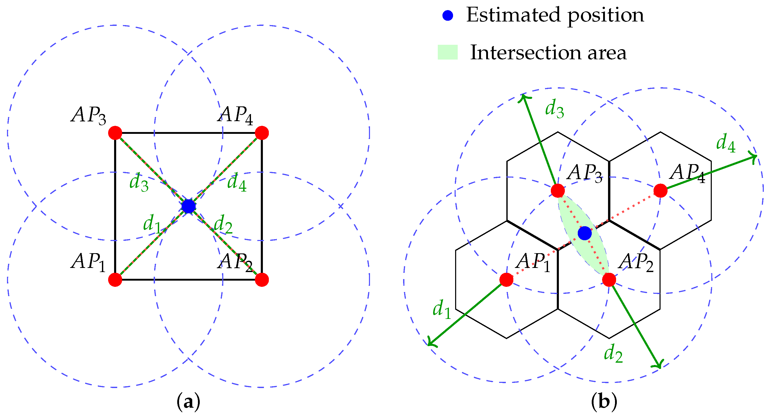
Beyond deployment considerations, the grid geometry has a direct impact on localization accuracy. In the rectangular architecture, reference nodes are placed at the corners of the grid, and the intersection occurs within a very small area or, ideally, at a single point. In contrast, the hexagonal grid architecture causes multilateration circles to intersect over an area rather than a single point, resulting in increased uncertainty and higher localization error.
Algorithm 1: Incremental virtual anchor generation using structured grid rules
Electronics 15 00584 i001
This geometric behavior is illustrated by the intersection shown in Figure 8. In the rectangular grid architecture, the distance circles associated with the surrounding anchors intersect within a compact region, resulting in a well-defined and stable position estimate. In contrast, in the hexagonal grid architecture, the distance circles overlap over a wider area due to the spatial arrangement of the anchors. This extended intersection region reflects increased geometric ambiguity, where small variations in RSSI-based distance estimates can lead to larger deviations in the estimated position, thereby contributing to the higher localization error observed for the hexagonal architecture.

5. Proposed Indoor Localization Application

5.1. Environment Setup

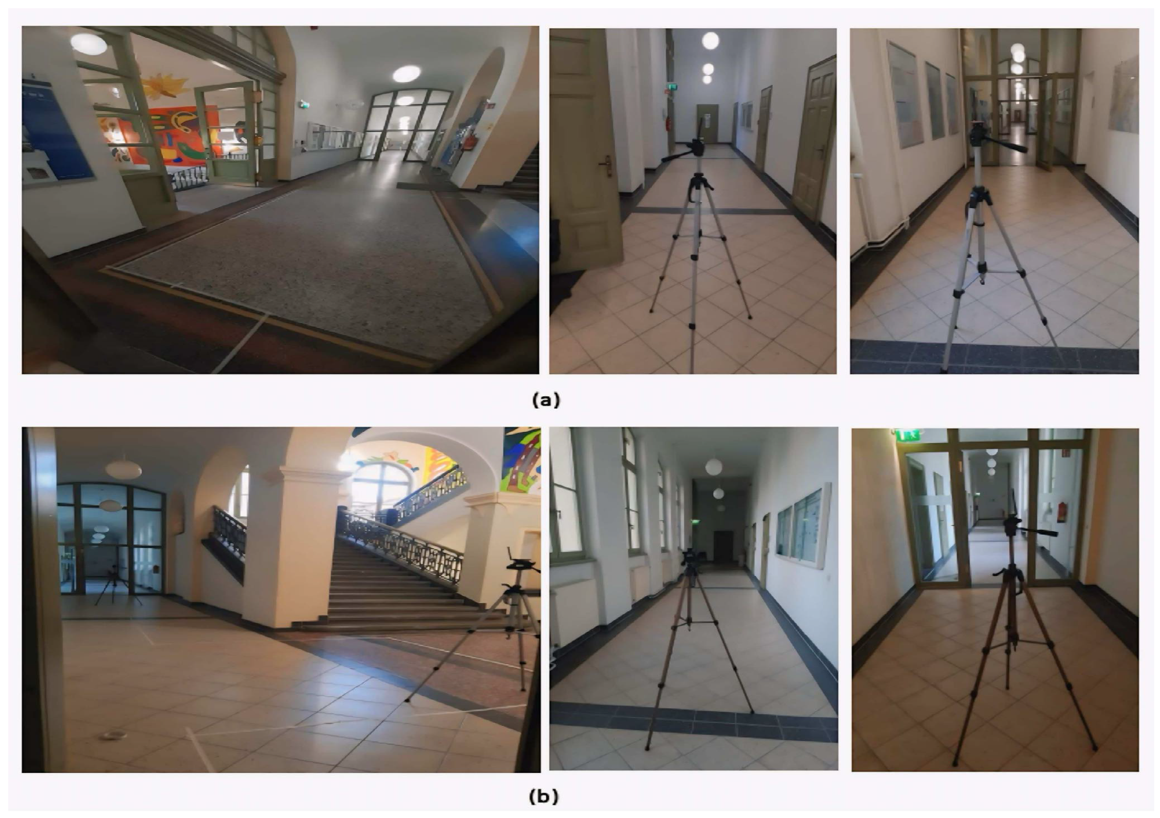
To test the proposed algorithm, experiments were conducted on two floors of the HTWK Leipzig building. The first floor, with a total area of approximately 196.5 m 2 , and the second floor, with a total area of 170.4 m 2 . The experimental setup included four anchors deployed in a real indoor environment to evaluate the accuracy of distance measurements. As summarized in Table 2, the anchors were strategically positioned along a corridor across two floors. Anchors 2 and 3 were located on the first floor, while anchors 4 and 5 were placed on the second floor. Based on the collected data, the path loss exponent η was found to vary between 1.61 and 3, reflecting the mixture of LOS and NLOS propagation conditions typically encountered in indoor environments [25]. The specific arrangement of the anchors and the corresponding environmental parameters are detailed in Figure 9 and Table 2. In addition, Figure 10 shows a highly obstructed indoor environment, characterized by dense laboratory furniture and metallic cabinets that strongly affect radio signal propagation. This configuration resulting in non-line of sight (NLOS) propagation, increased multipath effects, and higher attenuation.

5.2. Communication Protocol

The communication protocol is the most important part of the positioning system, enabling the target device and anchor nodes to interact efficiently. To adapt communication dynamically based on the mobility of the target node, we incorporate the algorithm proposed in [40]. Within this approach, transmission power is adjusted to selectively activate nodes based on target positions. A key element of this protocol is the use of WuRxs, which allow anchor nodes to remain in an ultra-low-power sleep state and be activated only on demand. The target device initiates the localization process by transmitting a wake-up call, which is detected by the WuRx of nearby anchors, triggering their main radio modules. This mechanism significantly reduces idle listening and energy consumption while enabling low-latency responses, which are essential for localization applications.
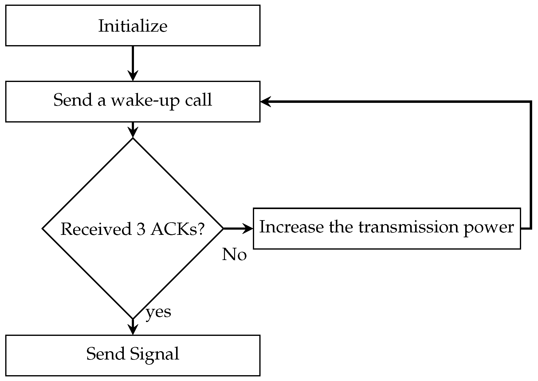
As illustrated in Figure 11, the target waits for acknowledgments (ACKs) from at least three activated anchors. Once these ACKs are received, the target transmits the collected data to a PC adapter connected to a laptop via UART. If an insufficient number of responses is obtained, the target increases its transmission power by 5 dBm and retries to ensure reliable connectivity. A machine learning model combined with multilateration then processes the received inputs in order to estimate the position of the target. The protocol initially operates with a default transmission power of 0 dBm .

5.3. Data Collection

The dataset includes the anchor IDs, the RSSI measurements, the environmental parameters, and the coordinates of the real anchors deployed in the test area. Recording temperature and humidity together with RSSI helps account for environmental variations that may influence signal propagation [26].
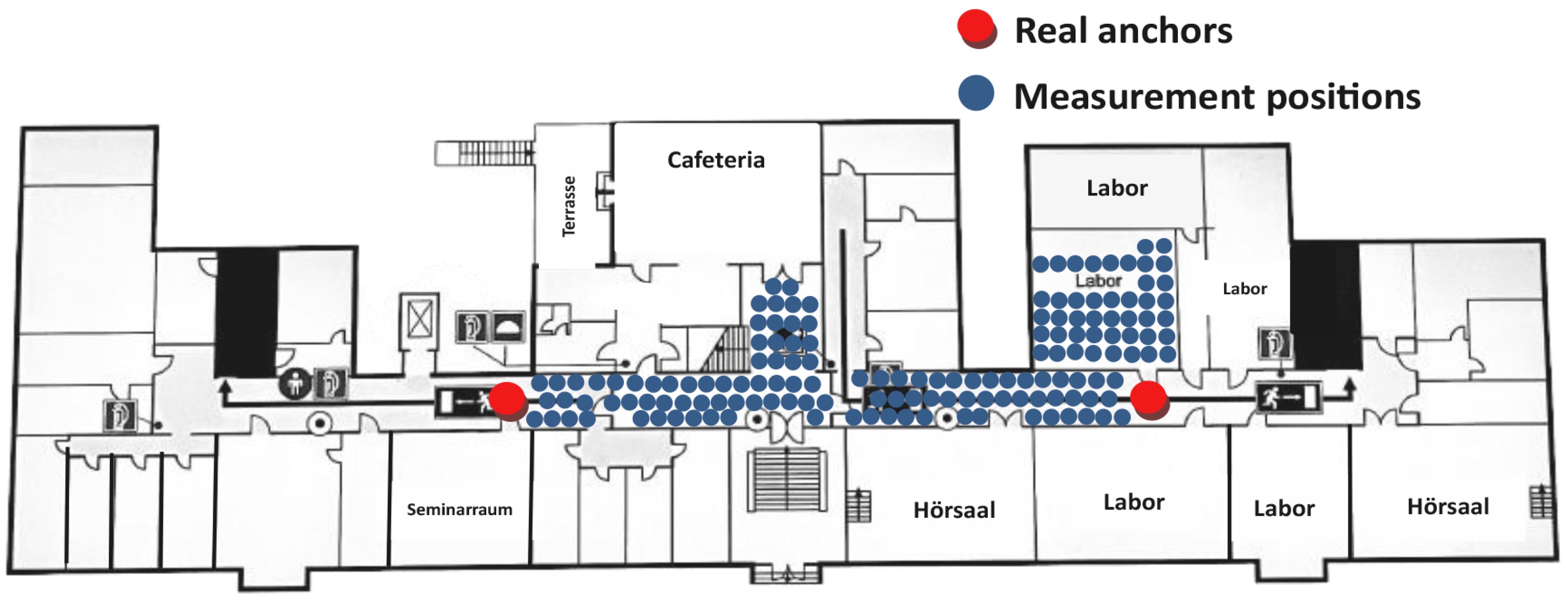
A total of 226 measurement positions were collected throughout the indoor environment. The measurement positions were spatially distributed across corridors, laboratory areas, and open spaces, ensuring representative coverage of the experimental layout. In particular, the laboratory areas contain dense furniture, structural walls, and measurement equipment, which introduce obstructions and multipath effects. As a result, several measurement positions experience NLOS propagation conditions. Accordingly, the estimated path loss exponent η was 2.66 on the first floor and 2.25 on the second floor, reflecting increased attenuation due to structural obstacles such as walls and floor separations.
The spatial distribution of the measurement positions for both floors is illustrated in Figure 12 and Figure 13, highlighting the coverage of NLOS propagation scenarios within the experimental environment. At each position, the target remained stationary for approximately 4 min, allowing the system to gather a sufficient number of samples and reduce the influence of short-term signal variations, resulting in representative RSSI, temperature, and humidity measurements.

5.4. Data Preprocessing

Data preprocessing is a critical step in preparing datasets for machine learning. It ensures that the data is clean, consistent, and fit for purpose [41]. This process involves several key techniques aimed at improving both data quality and model performance. One of the most important tasks is cleaning the data, which involves addressing missing values that could mislead the model and distort the results. We also check for data-type mismatches to ensure numeric values are correctly treated. Another important step in the process of cleaning data is dealing with outliers, defined as extreme values that differ significantly from the rest of the dataset. Outliers can reduce the reliability of models. Identifying and managing outliers helps ensure that the training data accurately reflects the underlying patterns of the problem we are trying to solve. Beyond cleaning, preprocessing also involves scaling features to make them comparable. A common approach is z-score standardization, which transforms the data to have a mean of 0 and a standard deviation of 1 [42].
z = x μ σ
where x is the original value, μ is the mean of the feature, σ is the standard deviation of the feature, and z is the standardized value. This process ensures that each feature contributes equally to the analysis or modeling process [43].

5.5. Proposed Offline Application

In the offline phase, two steps are performed. The first step involves predicting the features of the virtual anchors, while the second step involves predicting the distance between the target and the anchors using machine learning models. As illustrated in Figure 14, the process starts with data collection, where features such as anchor ID, RSSI, temperature, humidity, SQI, PQI, and Txp are gathered. The PQI and SQI are used to evaluate the reliability of preamble detection and the accuracy of signal synchronization. PQI reflects the quality of preamble detection by evaluating the stability of the received preamble sequence, while SQI measures the similarity between the received and expected synchronization words using cross-correlation, where a perfect match yields a value equal to eight times the synchronization length [44].
A data cleaning stage is then applied to ensure measurement reliability; during this stage, SQI, PQI, and Txp are discarded due to their instability and their limited contribution to improve distance estimation accuracy, while only ID, RSSI, temperature, and humidity are retained as input features for the learning process.
Virtual anchors are then positioned according to the selected grid architecture, and their features are predicted using a machine learning model. The resulting dataset, combining real and virtual anchors, is used to train different models for distance estimation. Finally, multilateration is applied for position estimation, and the models are evaluated and compared using performance metrics such as RMSE, MAE, and R2. Model performance is assessed through performance metrics using a dataset split into 70% training, 20% testing, and 10% validation sets. The comparison of models identifies the most effective one for accurate distance and coordinate prediction.

5.6. Proposed Online Application

The online phase enables real implementation with both real and virtual anchors while maintaining minimal latency.
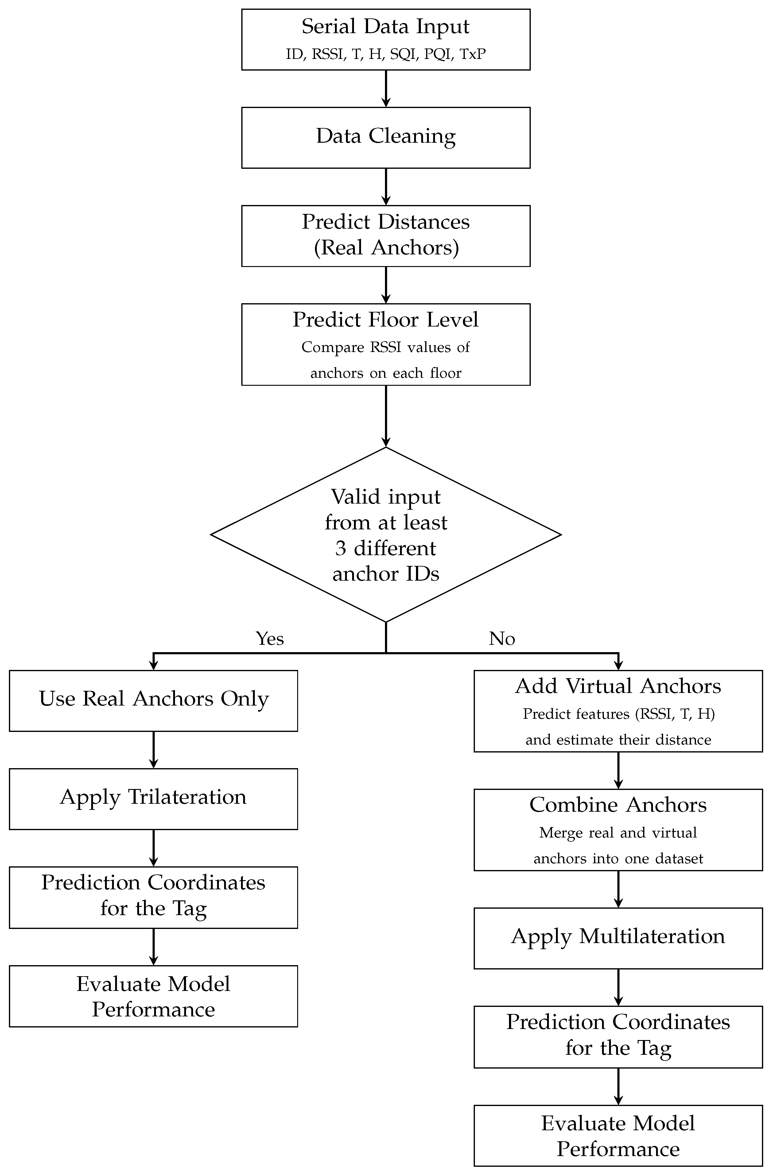
As shown in Figure 15, it begins with serial data acquisition, where measurements include anchor IDs, RSSI, temperature, and humidity, SQI, PQI, and Txp. After acquisition, data cleaning is performed to remove invalid or duplicate entries and ensure data consistency. Subsequently, the trained model from the offline phase is applied to estimate the distances between the tag and the available anchors based on signal characteristics. The floor level is inferred by comparing the RSSI values measured across different floors. Since the system operates at a transmission power of 0 dBm and covers multiple floors, the set of selected anchors may occasionally include anchors deployed on both floors, making direct floor identification based on anchor IDs unreliable. To resolve this ambiguity, the floor decision is performed by comparing the maximum RSSI values observed on each floor. The floor associated with the highest received signal strength is selected as the target floor. Once the floor is determined and measurements from at least three real anchors on the selected floor are available, the tag position is computed using trilateration, and the localization accuracy is subsequently evaluated. In cases where fewer than three real anchors are detected, virtual anchors are introduced. Their features and distances are predicted using the trained models, and they are combined with real anchors to enable reliable position estimation through multilateration. This phase differs from the offline phase because no model training or comparison is performed. The focus is on testing the selected model with incoming data to enable continuous and adaptive localization.

6. Results and Discussion

This study presents a comprehensive comparison of different machine learning models based on both error metrics and processing time. To minimize localization latency, multiple comparisons were conducted in the offline phase by varying the number of virtual anchors, aiming to identify the optimal model configuration for each grid architecture. This section also provides detailed insights into the performance of the system under realistic scenarios, demonstrating its potential for practical deployment.
We used performance measures for evaluation, including RMSE, MAE, and R2, to evaluate and characterize the effectiveness of our models. RMSE quantifies the average magnitude of prediction errors [45], while MAE represents the average of the absolute differences between predicted and actual values [46]. The coefficient of determination, R2, measures the proportion of variance in the dependent variable explained by the independent variables and ranges from 0 to 1. The mathematical definitions of RMSE, MAE, and R2 are provided in Equations (17), (18), and (19), respectively.
RMSE = 1 n i = 1 n ( y i y ^ i ) 2
MAE = 1 n i = 1 n y i y ^ i
R 2 = 1 i = 1 n ( y i y ^ i ) 2 i = 1 n ( y i y ¯ ) 2
where yi represents the observed (actual) value for each respective data point i. Additionally, y ^ i signifies the predicted value associated with each data point i. y ¯ is the average of all the observed target values.

6.1. Prediction of Virtual Anchors

For each network architecture, all anchors are assigned predefined coordinates together with a unique numerical identifier. In the experimental setup, two physical anchors are deployed on the first floor (IDs 2 and 3), while two physical anchors are installed on the second floor (IDs 4 and 5). Virtual anchors (VA) are progressively introduced to enhance spatial coverage and increase measurement density.
On the first floor, the addition of 12 virtual anchors results in IDs ranging from 6 to 17. For example, adding two VAs leads to IDs 6 and 7. Introducing 12 virtual anchors leads to IDs ranging from 18 to 29, where the addition of two VAs corresponds to IDs 18 and 19. This systematic indexing strategy ensures that physical and virtual anchors are clearly distinguished from each other across different floors.
The spatial locations of VAs are defined according to the selected architecture mentioned in Section 4.5, ensuring systematic numerical indexing, wide area coverage, and balanced spatial distribution. After defining the virtual anchor coordinates, the associated environmental features are predicted using a machine learning approach. In this study, the XGBoost model is employed to estimate the virtual anchor features, including RSSI, temperature, and humidity, using real measurements collected from physical anchors. The model is trained with a maximum tree depth of 7, a number of iterations of 200, and a learning rate of 0.5. XGBoost is selected for its robustness and high predictive accuracy when dealing with noisy indoor measurement data. After prediction, each virtual anchor is appended to the original dataset as a new data row containing its coordinates, unique ID, and predicted features. As virtual anchors are added incrementally, the size of the training dataset increases accordingly. This controlled data augmentation process significantly enriches the dataset and supports more robust learning and localization performance.
To analyze the impact of virtual anchors on data characteristics, kernel density estimation (KDE) is employed to compare the distributions of RSSI, temperature, and humidity before and after the introduction of virtual anchors. KDE estimates the probability density of data by smoothing measured samples. Given a set of samples x 1 , x 2 , , x n , the KDE is defined as [47]:
f ^ ( x ) = 1 n h i = 1 n K x x i h
where n denotes the number of samples, K ( · ) is the kernel function, and h is the bandwidth parameter controlling the smoothness of the estimated density.
K ( u ) = 1 2 π exp u 2 2
Figure 16 illustrates the kernel density estimation (KDE) of the RSSI, temperature, and humidity distributions for the initial dataset and the dataset with two virtual anchors. For RSSI, the probability density reaches a maximum of approximately 0.27–0.28 in the range of −52 to 50 dBm , indicating a high concentration of signal strength values within this interval. For temperature, the density exhibits a primary peak of approximately 0.9 around 21 °C to 22 °C, with a secondary peak observed near 24 °C. In the case of humidity, the maximum density is approximately 0.14–0.15, centered around 45–55%, reflecting the dominant range of humidity measurements. The KDE results show that the shapes of the RSSI, temperature, and humidity distributions after virtual anchor integration closely follow those of real anchors. This similarity confirms that virtual anchors emulate real anchor features, while KDE curves indicate increased data density and improved continuity of the feature space.

6.2. Distance Prediction Using Different Numbers of Virtual Anchors

During the offline phase, a hyperparameter tuning process was conducted to optimize the learning models, as described in Section 4.4. Key parameters, including tree depth, number of iterations, and learning rate, were adjusted within predefined ranges to ensure accurate predictions while maintaining computational efficiency and limiting overfitting. The performance of the machine learning models used in this study was evaluated through a systematic hyperparameter analysis. For CatBoost and XGBoost, parameters such as tree depth, number of iterations, and learning rate were tuned. In contrast, the RF model was evaluated by adjusting parameters, including tree depth and the number of trees. The results showed that increasing the tree depth reduced the prediction error up to an optimal value of 7. Similarly, model performance improved with the number of iterations up to around 200, after which further improvements were minimal. The learning rate also had a clear impact, with a value of 0.5 providing the lowest error. These trends were observed consistently for both rectangular and hexagonal architectures. Based on the optimized hyperparameter settings obtained, distance prediction is used to evaluate the impact of the number of VAs on indoor localization performance. Experiments are conducted for both rectangular and hexagonal grids with 2 to 12 VAs using the RF, CatBoost, and XGBoost models. For each architecture, the same anchor coordinates are employed. Table 3 and Table 4 present the RMSE values of each model in both architectural setups. For the rectangular grid architecture, the best results are achieved with XGBoost, and 10 added virtual anchors, with an RMSE of 2.02 m . This architecture outperforms the hexagonal grid architecture by 1.16 m for the same number of added virtual anchors. For all the configurations comparing the two architectures, XGBoost produced the best results for the rectangle grid architecture with 10 virtual anchors. Using the RF method increases the number of virtual anchors, reducing the RMSE from 3.07 m to 2.73 m when using the rectangular grid with two and ten virtual anchors, respectively. This demonstrates the importance of virtual anchors.
In contrast, the hexagonal configuration exhibits degraded performance with XGBoost as the number of anchors increases, with the RMSE increasing from 2.27 m at two anchors to 3.18 m at ten anchors, a degradation of 0.91 m . Testing the CatBoost model, an RMSE of 2.33 m was obtained with the rectangular grid architecture employing 10 anchors, while the hexagonal grid architecture yielded an RMSE of 3.30 m . RF shows smaller gains but still confirms the superiority of the rectangular grid.
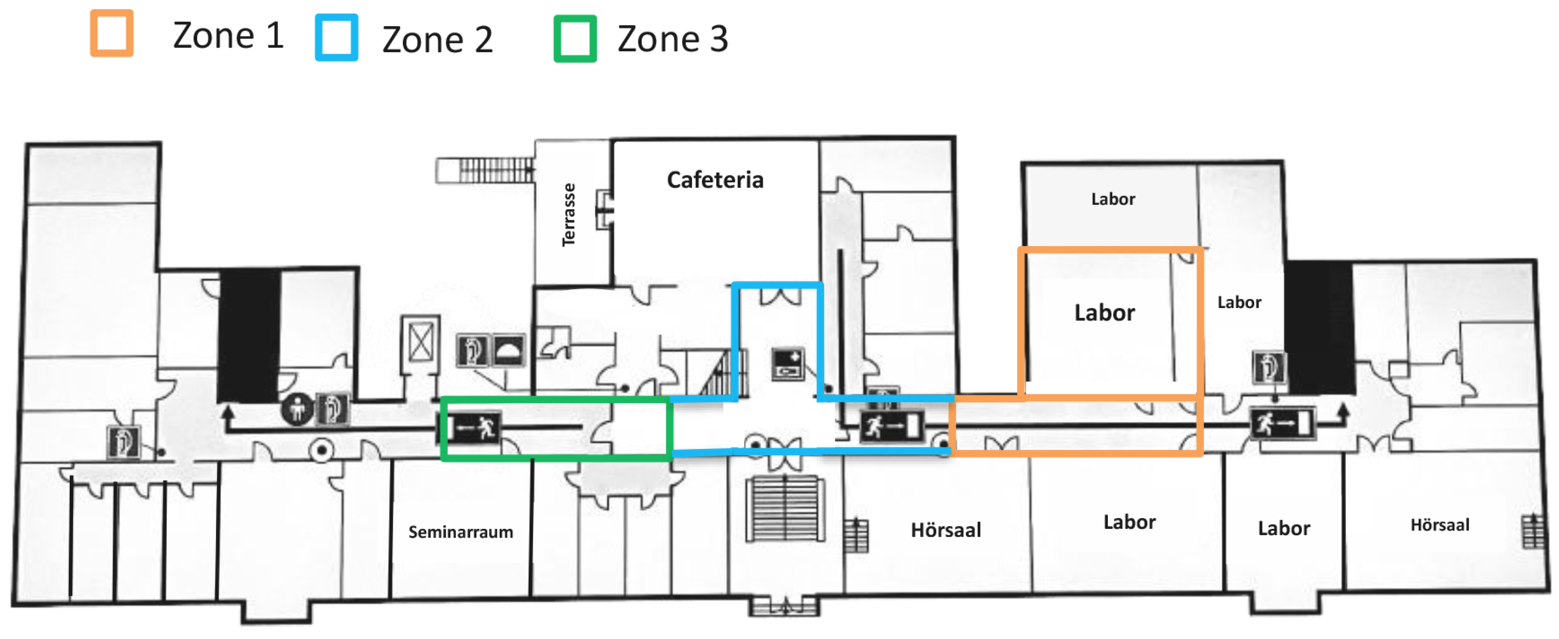
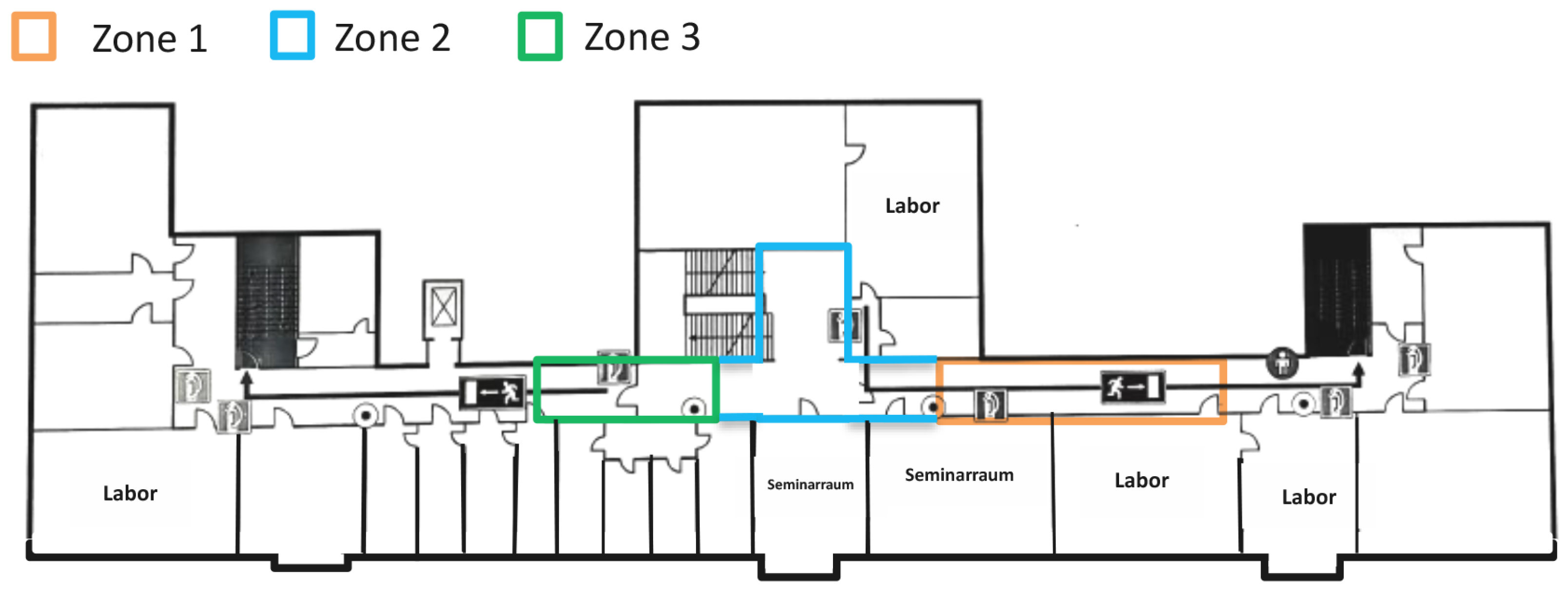
The RMSE fluctuations observed in Table 3 and Table 4 are explained by the zone-based analyses presented in Table 5 and Table 6, which characterize the RMSE behavior on floor 1 and floor 2 under different propagation conditions. To enable a detailed evaluation of RMSE variations, the deployment area on each floor is divided into three distinct zones, as illustrated by the zone layouts shown in Figure 17 and Figure 18. Specifically, the rectangular architecture with 12 virtual anchors is analyzed to clearly explain RMSE fluctuations across zones under LOS and NLOS conditions. On the first floor, zones 1 and 3 show the highest RMSE values of 3.45 m and 4.32 m, respectively. These zones are dominated by NLOS conditions, with path loss exponent values typically ranging from 2.10 to 2.65. This increases multipath effects and higher signal attenuation, resulting in increased RSSI variability and larger localization errors. In contrast, zone 2 on the first floor presents a mixture of LOS and NLOS conditions and achieves a lower RMSE of 2.52 m. On the second floor, zone 1, which is dominated by NLOS conditions, records a higher RMSE of 2.39 m. In contrast, zones 2 and 3, characterized by mixed LOS and NLOS propagation, achieve lower RMSE values of 1.82 m and 2.08 m, respectively. This behavior confirms that the observed RMSE fluctuations are mainly driven by variations in propagation conditions across zones.
Overall, while RMSE fluctuations are observed across zones and floors due to heterogeneous propagation environments, these variations do not affect the identification of the optimal configuration. They highlight the importance of carefully selecting the number of VAs to achieve efficient localization performance and confirm the selection of a configuration based on 10 VAs arranged in a rectangular grid. This conclusion is later validated by the multilateration results.
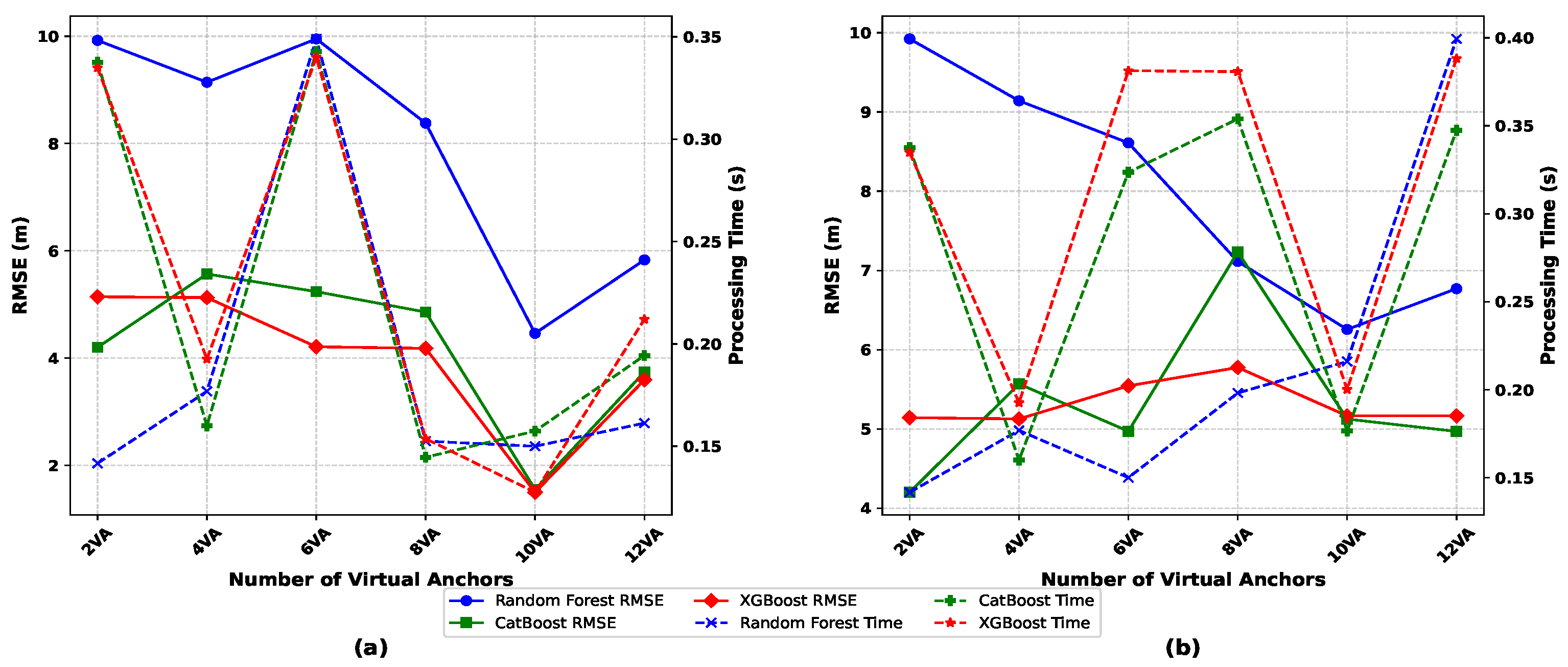
In order to analyze the results, a comparison of all configurations is presented in terms of error and processing time for localizing the target in different positions. These results, shown in Figure 19, present the stability of processing times. In the rectangular configuration, times remain stable between 0.15 s and 0.25 s , even as the number of anchors increases, while the hexagonal design shows greater fluctuations, reaching values of 0.40 s at 12 anchors. Notably, both architectures show that increasing the number of anchors above 10 degrades performance. Specifically, in the rectangular case, the RMSE increases from 1.49 m at 10 anchors to 3.80 m at 12 anchors, indicating redundancy and overfitting.
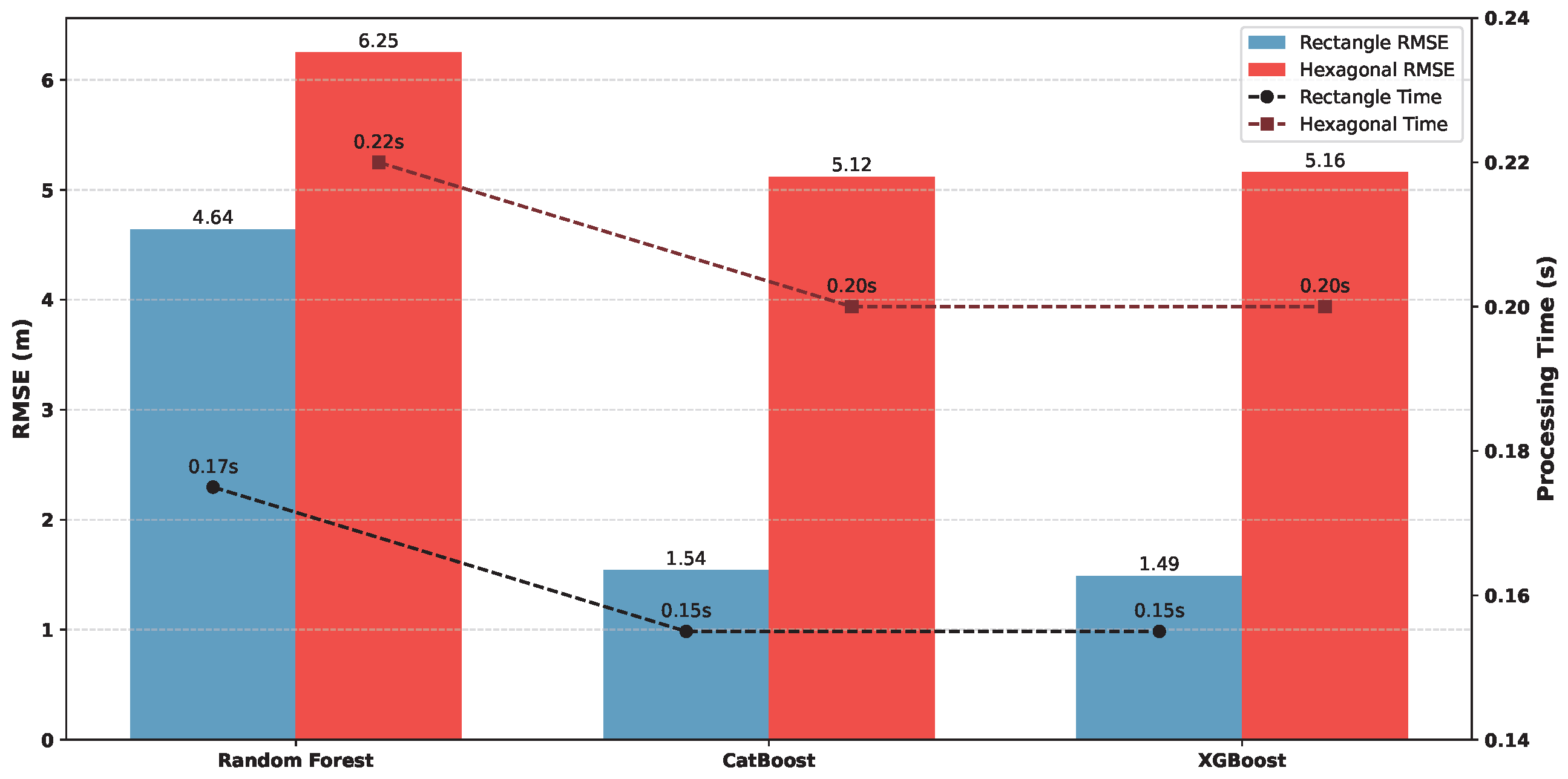
Therefore, based on the superior overall performance, we choose to proceed with 10 virtual anchors for both the rectangular and hexagonal architectures in all subsequent experiments. This allows for a consistent and reliable comparison of the two spatial configurations. While Figure 19 illustrates the behavior of the models across different numbers of virtual anchors, the results in Figure 20 focus specifically on the 10 VAs configuration, which provides the most stable and representative comparison.
Overall, the rectangular architecture with 10 virtual anchors provides the best balance between localization accuracy and computational efficiency. These results confirm that the rectangular architecture consistently outperforms the hexagonal architecture in terms of both accuracy and processing time. With CatBoost, the RMSE decreases from 5.12 m in the hexagonal case to 1.54 m in the rectangular case, representing an improvement of 3.58 m . Similarly, with XGBoost, the RMSE is reduced from 5.16 m in the hexagonal architecture to 1.49 m in the rectangular architecture. Even for the RF, which exhibited the highest errors overall, the rectangular grid achieves a 4.64 m RMSE compared to 6.25 m in the hexagonal case.

6.3. Performance Evaluation Using 10 Virtual Anchors

After identifying 10 virtual anchors as the optimal number, we focused the rest of the analysis on this fixed configuration to better understand the system behavior. This section conducts a detailed analysis using a validation dataset, which is composed of previously unseen data. This evaluation aims to assess the robustness of the system before the online testing phase. We provide a detailed evaluation of the predicted distance performance using 10 virtual anchors, comparing the rectangular and hexagonal architectures of the three selected machine learning models, RF, XGBoost, and CatBoost. The comparison is based on four key metrics, RMSE, MAE, coefficient of determination (R2), and processing time. These results provide insights into the influence of each architecture on the accuracy of the model and efficiency when the number of virtual anchors is kept constant. To compare the results, we used the test and validation datasets, which represent 20% and 10%, respectively.
As shown in Table 3 and Table 7, the rectangular architecture demonstrated better prediction accuracy, especially when using XGBoost. This model achieved the lowest RMSE and MAE, as well as the highest R2, indicating an excellent model fit and low prediction error, with values of 2.02 m , 1.01 m , and 0.92, respectively. In contrast, CatBoost showed slightly higher values where RMSE reached the value of 2.33 m , MAE was 1.59 m , and R2 was 0.90, while the RF performed significantly worse across all metrics.
In comparison, the results for the hexagonal architecture in Table 4 and Table 8 showed lower accuracy. The XGBoost model yielded an RMSE of 3.18 m , an MAE of 2.06 m , and an R2 value of 0.88. However, its performance was slightly lower than the rectangular grid configuration. CatBoost followed with an MAE of 1.59 m and R2 of 0.90, and RF showed the highest error levels and lowest R2. Among the two grid architectures, the RF model exhibited the weakest performance across all evaluation metrics, including MAE, RMSE, and R2. For the hexagonal grid architecture, the model produced values of 3.44 m for MAE, 4.64 m for RMSE, and 0.75 for R2. Performance improved for the rectangular grid architecture, with a reduction of 1.51 m in MAE and an increase of 0.10 in R2. Despite these improvements, it remained the least accurate model compared to the other approaches. While processing times were similar or slightly better in the hexagonal configuration, this small gain in speed did not make up for the lower accuracy of the predictions. Processing times remained within acceptable limits for all models, with XGBoost effectively balancing accuracy and speed. The validation results confirm the stability and robustness of XGBoost for all configurations of the test and validation datasets. After a comprehensive analysis of grid architectures, the number of virtual anchors, multilateration performance, and processing time, using the evaluation metrics MAE, RMSE, and R2 on both the validation and test datasets, the obtained results confirm the results observed in the simulations presented in [39]. This phase enabled the development of pretrained models that first predict the virtual anchor positions and subsequently estimate the distances used for multilateration-based target tracking. This step was essential for defining a robust model capable of maintaining stable performance under varying signal conditions, which are expected to occur during the online deployment phase. Based on the comparative evaluation of the rectangular and hexagonal architectures, as well as the evaluation of distance prediction and multilateration accuracy, the rectangular architecture provides more accurate and reliable localization results. In particular, the integration of the XGBoost model achieves a localization error of 1.49 m with an average processing time of approximately 0.15 s . Consequently, this configuration is selected for the online phase.

6.4. Performance Evaluation of the Online Process

This evaluation focuses on key performance metrics such as accuracy and processing speed. By analyzing these factors, we can determine the capability of the system to handle dynamic data inputs and its overall reliability in an online environment. This section provides detailed insights into how well the system performs under real-world conditions, ensuring its suitability for practical applications.
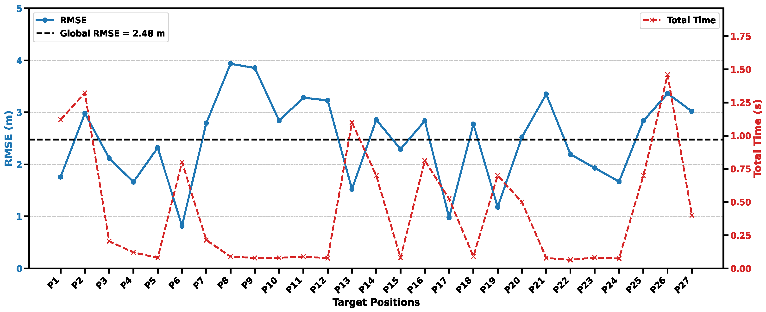
Figure 21 presents the results obtained from both floors, where RMSE varies across tested target positions, ranging from a minimum of 0.81 m to a maximum of 3.93 m , with an RMSE of 2.48 m . This distribution highlights the fundamental challenges of indoor environments, where signal propagation and anchor placement significantly impact positioning accuracy. In addition, processing time is analyzed to assess real implementation feasibility. The processing time remains low across most target positions, generally below 1.5 s .
Table 9 provides a statistical summary of the localization accuracy achieved using the XGBoost model. A closer examination of the reported error metrics indicates stable and reliable performance, with approximately 90% of the RMSE values remaining below 2.32 m and 70% below 2.10 m . These results confirm that the proposed approach maintains consistent localization accuracy under real implementation conditions.
The localization error statistics summarized in Table 10 enable a floor-level evaluation of system accuracy. Floor 1, covering an area of 196.5 m 2 , achieves an RMSE of 2.42 m . In contrast, floor 2, with a larger area of 170.4 m 2 , achieve an RMSE of 2.55 m . Focusing on the best performing localization results, 90% of the errors remain below 2.29 m for floor 1 and 2.32 m for floor 2, while 70% of the errors are below 2.05 m and 2.10 m , respectively. As discussed in Section 5.6, the proposed floor determination strategy enables the correct identification of the target floor before computing the target position. Compared with the studies discussed in Section 2 and Table 11, several limitations were found in previous works. UWB-based solutions, as reported in [15,18], present low localization errors ranging from 0.20 to 1.5 m . However, these approaches rely on costly UWB hardware and specific deployment strategies that limit scalability. The authors in [15] employ a single physical anchor but require up to 25 virtual anchors within a limited 6 × 6 m area. Consequently, this configuration exhibits limited scalability and is not well suited for large-scale, multi-floor indoor environments. RSSI-based approaches, as demonstrated in [16], can reduce hardware costs, but they still require four physical anchors and have been validated only in small and structured environments, including a 4 × 4 m room and a 22 × 9.3 m corridor. Although localization errors of 0.68 m and 1.77 m are achieved, respectively, the approach remains sensitive to environmental changes and lacks validation in larger indoor spaces. Similarly, ANN-based fingerprinting methods in [17] achieve low localization errors of 0.27 m . However, these results are obtained exclusively through simulations conducted in a single room scenario of 12.6 × 4.5 m . In addition, this approach requires extensive offline data collection and long training phases, which significantly restrict its applicability in dynamic and large-scale real-world environments. In contrast, our proposed system operates across two real floors with a total coverage of 366.9 m2 using only four physical anchors, while maintaining competitive accuracy with an offline RMSE of 1.49 m and an online RMSE of 2.48 m . By relying on low-cost RSSI measurements enhanced through machine learning-based virtual anchors and multilateration, the system achieves robust performance in realistic conditions. Furthermore, the system incorporates energy-efficient WuRx nodes, ensuring low energy consumption. These results demonstrate a practical and scalable alternative that overcomes the cost, coverage, and environmental limitations of state-of-the-art solutions.

7. Conclusions

Reducing deployment costs is critical for indoor localization technologies such as UWB and BLE, as these systems require additional hardware infrastructure. In this work, a balance was sought between cost-effectiveness, low energy consumption, and localization accuracy. This study was conducted through a multi-stage methodology designed to meet these objectives.
In the first stage, system deployment costs were reduced by using only four physical anchors to cover two floors with an area of 366.9 m2, complemented by the introduction of virtual anchors that share the same characteristics as real anchors. Predefined coordinates were assigned to each virtual anchor according to the selected grid architecture, with an ID. Using measurements from the real anchors, the virtual anchor features were predicted using XGBoost with 200 trees, a maximum depth of 7, and a learning rate of 0.5. After analyzing the resulting data distribution, this study proceeded to the second stage, which focused on determining the optimal number of virtual anchors.
In this stage, the number of active anchors was selected based on the chosen grid architecture. Two different architectures were compared in terms of processing time and localization accuracy. The number of virtual anchors was gradually increased for each architecture from 2 VA to 12 VA, and performance was evaluated using RMSE, MAE, and R2. Following an extensive analysis, a rectangular grid with 10 virtual anchors was identified as the optimal configuration. The best performance was again obtained using XGBoost with 200 trees, a maximum depth of 7, and a learning rate of 0.5. This configuration achieved an RMSE of 1.49 m , with an average processing time of approximately 0.15 s for the offline phase. To reduce energy consumption, wake-up receiver nodes were employed in combination with a dedicated communication protocol designed to minimize the number of active nodes. A variable transmission power strategy was used to dynamically activate anchors according to the mobility of the target, thereby improving energy efficiency while maintaining localization performance. By combining the proposed communication protocol with a rectangular grid architecture using ten virtual anchors, four real anchors, and the pretrained model, the system achieved an RMSE of 2.48 m . This result confirms the practical viability of the proposed approach for indoor localization scenarios.
As future work, virtual anchors will be treated as adaptive design parameters, where both their number and spatial placement are dynamically optimized to suit different building layouts, area sizes, and multi-floor environments. In addition, future investigations will aim to further align the distributions of virtual anchor features with those of real measurements, ensuring a closer match to real-world signal and environmental variability. Such an adaptive and flexible virtual anchor strategy is expected to enhance system scalability, robustness, and generalization across diverse indoor scenarios.

Author Contributions

S.C., conceptualization, methodology, original draft writing, visualization, and editing; A.C., reviewing, editing, and visualization; R.S., reviewing, editing, and visualization; S.S., reviewing, editing, and visualization; A.F. and F.D., writing paragraphs, reviewing, and editing. All authors have read and agreed to the published version of the manuscript.

Funding

This research received no external funding.

Institutional Review Board Statement

Not applicable.

Informed Consent Statement

Not applicable.

Data Availability Statement

Data are contained within the article.

Acknowledgments

We acknowledge support by the Open Access Publication Funds of the Leipzig University of Applied Sciences. This research was performed at the Leipzig University of Applied Sciences (HTWK).

Conflicts of Interest

The authors declare no conflicts of interest.

Abbreviations

The following abbreviations are used in this manuscript:
IPSsIndoor Positioning Systems
GNSSsGlobal Navigation Satellite Systems
GPSGlobal Positioning System
TOATime of Arrival
TDOATime Difference of Arrival
AOAAngle of Arrival
RSSIReceived signal strength indication
VAsVirtual Anchors
ANNsArtificial Neural Networks
WuRxWake-up receiver
WuPTWake-up Packet
LOSLine of sight
NLOSNon-line of sight
UWBUltra-Wide Band
XGBoostExtreme Gradient Boosting
CatBoostCategory Boosting
RFRandom Forest
PQIPreamble Quality Indicator
SQISynchronization Quality Indicator
TxpTransmission Power
RMSERoot Mean Square Error
MAEMean Absolute Error

References

  1. Gu, Y.; Lo, A.; Niemegeers, I. A survey of indoor positioning systems for wireless personal networks. IEEE Commun. Surv. Tutorials 2009, 11, 13–32. [Google Scholar] [CrossRef]
  2. Yassin, A.; Nasser, Y.; Awad, M.; Al-Dubai, A.; Liu, R.; Yuen, C.; Raulefs, R.; Aboutanios, E. Recent advances in indoor localization: A survey on theoretical approaches and applications. IEEE Commun. Surv. Tutorials 2016, 19, 1327–1346. [Google Scholar] [CrossRef]
  3. Pan, M.; Liu, P.; Liu, S.; Qi, W.; Huang, Y.; You, X.; Jia, X.; Li, X. Efficient joint DOA and TOA estimation for indoor positioning with 5G picocell base stations. IEEE Trans. Instrum. Meas. 2022, 71, 8005219. [Google Scholar] [CrossRef]
  4. Yimwadsana, B.; Serey, V.; Sanghlao, S. Performance analysis of an AoA-based Wi-Fi indoor positioning system. In Proceedings of the 2019 19th International Symposium on Communications and Information Technologies (ISCIT); IEEE: Piscataway, NJ, USA, 2019; pp. 36–41. [Google Scholar]
  5. Guidara, A.; Derbel, F. A real-time indoor localization platform based on wireless sensor networks. In Proceedings of the 2015 IEEE 12th International Multi-Conference on Systems, Signals & Devices (SSD15); IEEE: Piscataway, NJ, USA, 2015; pp. 1–8. [Google Scholar]
  6. Cheng, Y.; Zhou, T. UWB indoor positioning algorithm based on TDOA technology. In Proceedings of the 2019 10th International Conference on Information Technology in Medicine and Education (ITME); IEEE: Piscataway, NJ, USA, 2019; pp. 777–782. [Google Scholar]
  7. Gezici, S. A survey on wireless position estimation. Wirel. Pers. Commun. 2008, 44, 263–282. [Google Scholar] [CrossRef]
  8. Hailu, T.G.; Guo, X.; Si, H.; Li, L.; Zhang, Y. Theories and methods for indoor positioning systems: A comparative analysis, challenges, and prospective measures. Sensors 2024, 24, 6876. [Google Scholar] [CrossRef]
  9. Wang, J.; Park, J. An enhanced indoor positioning algorithm based on fingerprint using fine-grained csi and rssi measurements of ieee 802.11 n wlan. Sensors 2021, 21, 2769. [Google Scholar]
  10. Zafari, F.; Gkelias, A.; Leung, K.K. A survey of indoor localization systems and technologies. IEEE Commun. Surv. Tutorials 2019, 21, 2568–2599. [Google Scholar] [CrossRef]
  11. He, S.; Chan, S.H.G. Wi-Fi fingerprint-based indoor positioning: Recent advances and comparisons. IEEE Commun. Surv. Tutorials 2015, 18, 466–490. [Google Scholar] [CrossRef]
  12. Hoffmann, E.J.; Werner, M.; Schauer, L. Indoor navigation using virtual anchor points. In Proceedings of the 2016 European Navigation Conference (ENC); IEEE: Piscataway, NJ, USA, 2016; pp. 1–8. [Google Scholar]
  13. Esheh, J.; Affes, S. Effectiveness of data augmentation for localization in WSNs using deep learning for the Internet of Things. Sensors 2024, 24, 430. [Google Scholar] [CrossRef]
  14. Limkar, S.; Ashok, W.V.; Wadne, V.; Wagh, S.K.; Wagh, K.; Kumar, A. Energy-Efficient Localization Techniques for Wireless Sensor Networks in Indoor IoT Environments. J. Electr. Syst. 2023, 19, 47. [Google Scholar] [CrossRef]
  15. Choi, H.B.; Lim, K.W.; Ko, Y.B. Improved virtual anchor selection for AR-assisted sensor positioning in harsh indoor conditions. In Proceedings of the 2020 Global Internet of Things Summit (GIoTS); IEEE: Piscataway, NJ, USA, 2020; pp. 1–6. [Google Scholar]
  16. Booranawong, A.; Sengchuai, K.; Buranapanichkit, D.; Jindapetch, N.; Saito, H. RSSI-based indoor localization using multi-lateration with zone selection and virtual position-based compensation methods. IEEE Access 2021, 9, 46223–46239. [Google Scholar] [CrossRef]
  17. Pedrollo, G.; Konzen, A.A.; de Morais, W.O.; Pignaton de Freitas, E. Using smart virtual-sensor nodes to improve the robustness of indoor localization systems. Sensors 2021, 21, 3912. [Google Scholar] [CrossRef] [PubMed]
  18. Großwindhager, B.; Rath, M.; Kulmer, J.; Bakr, M.S.; Boano, C.A.; Witrisal, K.; Römer, K. SALMA: UWB-based single-anchor localization system using multipath assistance. In Proceedings of the 16th ACM Conference on Embedded Networked Sensor Systems, Shenzhen, China, 4–7 November 2018; pp. 132–144. [Google Scholar]
  19. Li, J.; Yu, S.; Wei, Z.; Zhou, Z. An Enhanced ZigBee-Based Indoor Localization Method Using Multi-Stage RSSI Filtering and LQI-Aware MLE. Sensors 2025, 25, 2947. [Google Scholar] [CrossRef] [PubMed]
  20. Shang, F.; Jiang, Y.; Xiong, A.; Su, W.; He, L. A node localization algorithm based on multi-granularity regional division and the lagrange multiplier method in wireless sensor networks. Sensors 2016, 16, 1934. [Google Scholar] [CrossRef]
  21. Meissner, P.; Gigl, T.; Witrisal, K. UWB sequential Monte Carlo positioning using virtual anchors. In Proceedings of the 2010 International Conference on Indoor Positioning and Indoor Navigation; IEEE: Piscataway, NJ, USA, 2010; pp. 1–10. [Google Scholar]
  22. Leitinger, E.; Fröhle, M.; Meissner, P.; Witrisal, K. Multipath-assisted maximum-likelihood indoor positioning using UWB signals. In Proceedings of the 2014 IEEE International Conference on Communications Workshops (ICC); IEEE: Piscataway, NJ, USA, 2014; pp. 170–175. [Google Scholar]
  23. Fromm, R.; Kanoun, O.; Derbel, F. An improved wake-up receiver based on the optimization of low-frequency pattern matchers. Sensors 2023, 23, 8188. [Google Scholar] [CrossRef]
  24. Schott, L.; Fromm, R.; Bouattour, G.; Kanoun, O.; Derbel, F. Analytical and experimental performance analysis of enhanced wake-up receivers based on low-power base-band amplifiers. Sensors 2022, 22, 2169. [Google Scholar] [CrossRef]
  25. Souissi, R.; Ktata, I.; Sahnoun, S.; Fakhfakh, A.; Derbel, F. Improved rssi distribution for indoor localization application based on real data measurements. In Proceedings of the 2024 21st International Multi-Conference on Systems, Signals & Devices (SSD); IEEE: Piscataway, NJ, USA, 2024; pp. 486–491. [Google Scholar]
  26. Guidara, A.; Fersi, G.; Derbel, F.; Jemaa, M.B. Impacts of Temperature and Humidity variations on RSSI in indoor Wireless Sensor Networks. Procedia Comput. Sci. 2018, 126, 1072–1081. [Google Scholar] [CrossRef]
  27. Naghdi, S.; O’Keefe, K. Combining multichannel RSSI and vision with artificial neural networks to improve BLE trilateration. Sensors 2022, 22, 4320. [Google Scholar] [CrossRef]
  28. Du, J.; Yuan, C.; Yue, M.; Ma, T. A novel localization algorithm based on RSSI and multilateration for indoor environments. Electronics 2022, 11, 289. [Google Scholar] [CrossRef]
  29. Cengiz, K. Comprehensive analysis on least-squares lateration for indoor positioning systems. IEEE Internet Things J. 2020, 8, 2842–2856. [Google Scholar] [CrossRef]
  30. Rathnayake, R.M.M.R.; Maduranga, M.W.P.; Tilwari, V.; Dissanayake, M.B. RSSI and Machine Learning-Based Indoor Localization Systems for Smart Cities. Eng 2023, 4, 1468–1494. [Google Scholar] [CrossRef]
  31. Breiman, L. Random forests. Mach. Learn. 2001, 45, 5–32. [Google Scholar] [CrossRef]
  32. Li, X.; Wen, Z.; Su, H. An approach using random forest intelligent algorithm to construct a monitoring model for dam safety. Eng. Comput. 2021, 37, 39–56. [Google Scholar] [CrossRef]
  33. Yuliana, H.; Basuki, S.; Hidayat, M.R.; Charisma, A.; Vidyaningtyas, H. Hyperparameter Optimization of Random Forest Algorithm to Enhance Performance Metric Evaluation of 5G Coverage Prediction. Bul. Pos Dan Telekomun. 2024, 22, 75–90. [Google Scholar]
  34. Prokhorenkova, L.; Gusev, G.; Vorobev, A.; Dorogush, A.V.; Gulin, A. CatBoost: Unbiased boosting with categorical features. In Proceedings of the 32nd International Conference on Neural Information Processing Systems, Montréal, QC, Canada, 3–8 December 2018. [Google Scholar]
  35. Hancock, J.; Khoshgoftaar, T. CatBoost for big data: An interdisciplinary review. J. Big Data 2020, 7, 94. [Google Scholar] [CrossRef]
  36. Elmasry, N.; Elshaarawy, M. Hybrid metaheuristic optimized Catboost models for construction cost estimation of concrete solid slabs. Sci. Rep. 2025, 15, 21612. [Google Scholar] [CrossRef]
  37. Chen, M.; Meng, X.; Kan, G.; Wang, J.; Li, G.; Liu, B.; Liu, C.; Liu, Y.; Liu, Y.; Lu, J. Predicting the sound speed of seafloor sediments in the east China sea based on an XGBoost algorithm. J. Mar. Sci. Eng. 2022, 10, 1366. [Google Scholar] [CrossRef]
  38. Verma, V. Exploring Key XGBoost Hyperparameters: A Study on Optimal Search Spaces and Practical Recommendations for Regression and Classification. Int. J. All Res. Educ. Sci. Methods (IJARESM) 2024, 12, 2455–6211. [Google Scholar] [CrossRef]
  39. Souissi, R.; Ktata, I.; Sahnoun, S.; Fakhfakh, A.; Derbel, F. Analysis of Different Architectures for RSSI Based Indoor Localization using Trilateration Technique. In Proceedings of the 2024 IEEE 4th International Maghreb Meeting of the Conference on Sciences and Techniques of Automatic Control and Computer Engineering (MI-STA); IEEE: Piscataway, NJ, USA, 2024; pp. 446–451. [Google Scholar]
  40. Souissi, R.; Sahnoun, S.; Baazaoui, M.K.; Fromm, R.; Fakhfakh, A.; Derbel, F. A self-localization algorithm for mobile targets in indoor wireless sensor networks using wake-up media access control protocol. Sensors 2024, 24, 802. [Google Scholar] [CrossRef]
  41. García, S.; Luengo, J.; Herrera, F. Data Preprocessing in Data Mining; Springer: Cham, Switzerland, 2015; Volume 72. [Google Scholar]
  42. Hastie, T.; Tibshirani, R.; Friedman, J. The Elements of Statistical Learning; Springer: Berlin/Heidelberg, Germany, 2009. [Google Scholar]
  43. Yaro, A.S.; Maly, F.; Prazak, P. Outlier detection in time-series receive signal strength observation using Z-score method with S n scale estimator for indoor localization. Appl. Sci. 2023, 13, 3900. [Google Scholar] [CrossRef]
  44. STMicroelectronics. SPIRIT1 Low Data Rate RF Transceiver Datasheet. Available online: https://www.mouser.in/pdfDocs/spirit1.pdf (accessed on 1 January 2026).
  45. Chiu, C.C.; Wu, H.Y.; Chen, P.H.; Chao, C.E.; Lim, E.H. Indoor Localization Using 6G Time-Domain Feature and Deep Learning. Electronics 2025, 14, 1870. [Google Scholar] [CrossRef]
  46. Chai, T.; Draxler, R.R. Root mean square error (RMSE) or mean absolute error (MAE)?—Arguments against avoiding RMSE in the literature. Geosci. Model Dev. 2014, 7, 1247–1250. [Google Scholar] [CrossRef]
  47. Parzen, E. On estimation of a probability density function and mode. Ann. Math. Stat. 1962, 33, 1065–1076. [Google Scholar] [CrossRef]
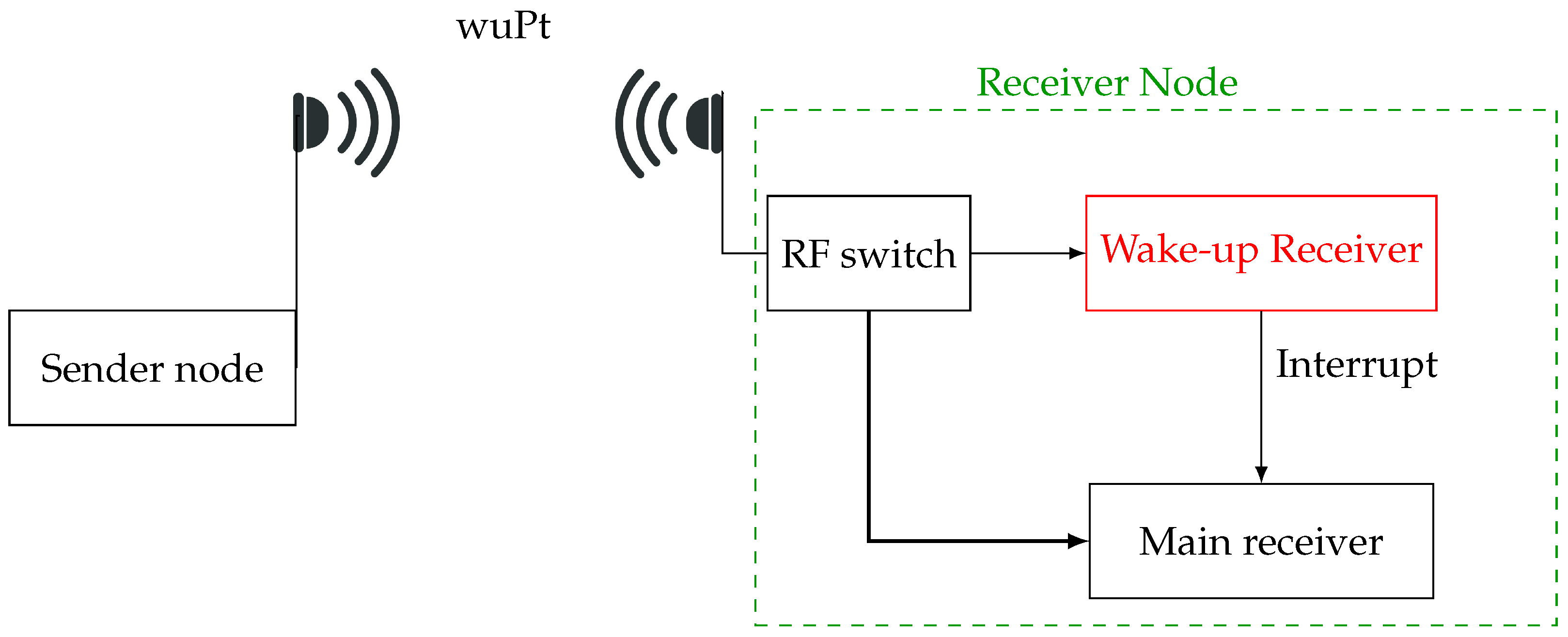
Figure 1. WuPT communication from a sender node to a receiver node based on wake-up receiver.
Electronics 15 00584 g001
Figure 2. Schematic diagram illustrating mulilateration.
Electronics 15 00584 g002
Figure 3. Virtual anchor feature prediction and integration into multilateration.
Electronics 15 00584 g003
Figure 4. The structure of the Random Forest algorithm.
Electronics 15 00584 g004
Figure 5. The structure of the CaBoost algorithm.
Electronics 15 00584 g005
Figure 6. The structure of the XGBoost algorithm.
Electronics 15 00584 g006
Figure 7. Rectangular and hexagonal grid architectures.
Electronics 15 00584 g007
Figure 8. Localization using multilateration in different architectures (a) Position estimation using a rectangle grid. (b) Position estimation using a hexagonal grid.
Electronics 15 00584 g008
Figure 9. Real measurement environment. (a) The first floor. (b) The second floor.
Electronics 15 00584 g009
Figure 10. Example of the tested laboratory environment.
Electronics 15 00584 g010
Figure 11. Used communication protocol.
Electronics 15 00584 g011
Figure 12. Spatial distribution of the measurement positions on the first floor of the experimental environment.
Electronics 15 00584 g012
Figure 13. Spatial distribution of the measurement positions on the second floor of the experimental environment.
Electronics 15 00584 g013
Figure 14. Flow chart of the proposed offline algorithm.
Electronics 15 00584 g014
Figure 15. Flow chart of the proposed online algorithm.
Electronics 15 00584 g015
Figure 16. Kernel density analysis before and after two virtual anchor integration. (a) KDE of RSSI. (b) KDE of temperature. (c) KDE of humidity.
Electronics 15 00584 g016
Figure 17. Zone map of the experimental area on the first floor.
Electronics 15 00584 g017
Figure 18. Zone map of the experimental area on the second floor.
Electronics 15 00584 g018
Figure 19. RMSE and processing time using multilateration with virtual anchors in both architectures. (a) Rectangle architecture. (b) Hexagonal architecture.
Electronics 15 00584 g019
Figure 20. Performance metrics using multilateration across 10 virtual anchors for rectangular architecture.
Electronics 15 00584 g020
Figure 21. Variation in RMSE and processing time based on real implementation.
Electronics 15 00584 g021
Table 1. A performance review of studies using virtual anchors.
ReferenceTechnologiesAlgorithmsNumber of Physical AnchorsNumber of Virtual AnchorsTested AreaDeployment TypeError
[15]UWBNot defined125Open space: 6 m × 6 m Office: 6 m × 6 m Real implementationOpen space: 0.8 m
Office: 1.5 m
[16]RSSI,
ZigBee (2.4 Ghz)
Multilateration
Not defined412
(3 per zone)
Room: 4 m × 4 m Corridor: 22 m × 9.3 m Real implementationRoom: 0.68 m
Corridor: 1.77 m
[17]RSSI,
Fingerprinting
ANN22 12.6 m × 4.5 m SimulationX-axis: 0.27 m
Y-axis: 0.28 m
[18]UWBNot defined14Room A:
31.6 m 2
Room B:
46.7 m 2
Real implementationRoom A: 0.20 m
Room B: 0.445 m
Table 2. Position of anchors in real environment.
Anchor NumberPositions (x, y)Floor
2(1.56 m, 15.54 m)1
3(1.54 m, 53.82 m)1
4(1.44 m, 43.76 m)2
5(1.29 m, 19.48 m)2
Table 3. Performance comparison of distance prediction error metrics using different numbers of virtual anchors in the rectangular architecture.
Number of Virtual Anchors24681012
RF (m)3.073.873.584.392.734.61
CatBoost (m)2.402.652.752.882.332.85
XGBoost (m)2.262.672.622.842.022.79
Table 4. Performance comparison of distance prediction error metrics using different numbers of virtual anchors in the hexagonal architecture.
Number of Virtual Anchors24681012
RF (m)3.074.124.033.754.644.64
CatBoost (m)2.132.872.674.333.305.52
XGBoost (m)2.272.852.834.183.186.19
Table 5. Zone-based RMSE fluctuation analysis under different propagation conditions on floor 1 using 12 VAs.
ZoneDistance Range Between VA and Target (m)Path Loss Exponent η RMSE (m)Environment Type
Zone 14.33–252.10–2.353.45NLOS
Zone 24.33–15.891.81–2.782.52NLOS, LOS
Zone 31.33–17.582.10–2.654.32NLOS
Table 6. Zone-based RMSE fluctuation analysis under different propagation conditions on floor 2 using 12 VAs.
ZoneDistance Range Between VA and Target (m)Path Loss Exponent η RMSE (m)Environment Type
Zone 15.91–19.952.10–2.232.39NLOS
Zone 21.52–11.891.68–21.82LOS
Zone 36.59–14.071.84–1.932.08LOS
Table 7. Performance comparison of distance prediction error metrics using a rectangular grid architecture.
AI AlgorithmsModelMetricsResults
RFTest DatasetMAE1.93 m
R20.86
Validation DatasetMAE1.96 m
R20.85
CatBoostTest DatasetMAE1.59 m
R20.90
Validation DatasetMAE1.61 m
R20.89
XGBoostTest DatasetMAE1.01 m
R20.92
Validation DatasetMAE1.04 m
R20.92
Table 8. Performance comparison of distance prediction error metrics using a hexagonal grid architecture.
AI AlgorithmsModelMetricsResults
RFTest DatasetMAE3.44 m
R20.76
Validation DatasetMAE3.48 m
R20.75
CatBoostTest DatasetMAE2.20 m
R20.85
Validation DatasetMAE2.25 m
R20.84
XGBoostTest DatasetMAE2.06 m
R20.88
Validation DatasetMAE2.09 m
R20.88
Table 9. RMSE performance analysis of the proposed indoor localization system.
ModelRMSE (m)Min RMSE (m)Max RMSE (m)90% RMSE (m)70% RMSE (m)
XGBoost2.480.813.932.322.10
Table 10. RMSE performance analysis of the proposed indoor localization system per floor.
FloorNumber of PositionsArea (m2)RMSE (m)Min RMSE (m)Max RMSE (m)90% RMSE (m)70% RMSE (m)
Floor 114196.52.420.983.362.292.05
Floor 213170.42.550.813.932.322.10
Table 11. Comparative evaluation with existing indoor positioning technologies.
ReferenceTechnologyHardware CostReal AnchorsTested AreaAccuracy
[18]UWBHigh1Room A: 31.6 m 2
Room B: 46.7 m 2
Room A: 0.20 m
Room B: 0.445 m
[15]UWBHigh1Open space: 6 m × 6 m Office: 6 m × 6 m Open space: 0.8 m
Office: 1.5 m
[16]RSSI MultilaterationLow4Room: 4 × 4 m 2 Corridor: 22 × 9.3 m Room: 0.68 m
Corridor: 1.77 m
[17]RSSI, ZigBee (2.4 GHz)
Multilateration
Low2 12.6 × 4.5 m X-axis: 0.27 m
Y-axis: 0.28 m
This workRSSI, WuRxLow4366.9 m2
2 floors
Offline: 1.49 m
Online: 2.48 m
Disclaimer/Publisher’s Note: The statements, opinions and data contained in all publications are solely those of the individual author(s) and contributor(s) and not of MDPI and/or the editor(s). MDPI and/or the editor(s) disclaim responsibility for any injury to people or property resulting from any ideas, methods, instructions or products referred to in the content.