Research on the Range Parameter Estimation Method of Low Signal-To-Background Ratio GM-APD LiDAR Based on Multi-Scale Tracking Differentiator

Abstract

To address the issue of the Geiger-mode Avalanche Photodiode (GM-APD) LiDAR’s echo being easily overwhelmed by strong noise under low signal-to-background ratio conditions, leading to degraded performance in range parameter estimation and low target restoration accuracy, this paper proposes a range parameter estimation method based on multi-scale tracking differentiator. This method eliminates the reliance on complex statistical models and spatial prior information and uses a nonlinear dynamic tracking mechanism to extract target information. Firstly, a dual-scale tracking differentiator system is constructed, where the large-scale factor captures the transient mutation characteristics of the echo signal, and the small-scale factor estimates the overall evolution trend of the signal. Secondly, the difference between the dual-scale outputs is obtained to acquire the residual signal, and nonlinear mapping enhancement is performed in combination with the photon trigger probability characteristics to deeply suppress noise and highlight the target peak. Finally, the peak threshold method is used to complete the range calculation. Simulation results show that when the SBR = 0.06, compared with typical methods such as the neighborhood kernel density method, the method in this paper is more robust, the root mean square error of the range estimation is reduced by at least 38.35%, and the target restoration degree is improved by at least 19.99%, which provides a highly efficient way for high-fidelity single-photon three-dimensional imaging and target detection under strong noise.

1. Introduction

Geiger-mode Avalanche Photodiode LiDAR (GM-APD), a transformative photon-counting technology capable of single-photon detection, with its single-photon-level detection sensitivity, picosecond-level time resolution and all-weather operation capability, has broad application prospects in fields such as autonomous driving and terrain mapping [1]. However, in Geiger mode, the detector only records the trigger time of the first photon in each emission cycle [2]. In a strong noise environment with extremely low signal-to-background ratio (SBR ≤ 1) [3], Signal-to-background ratio (SBR) is defined as the number of signal photons divided by the number of background noise photons, noise photons are highly likely to trigger the detector before the target photons, causing the echo signal to be severely submerged. As a result, the performance of range parameter estimation using traditional methods such as peak threshold [4] or maximum likelihood estimation [5] degrades sharply.

The contribution of this article is a dual-scale tracking differentiator combined with a nonlinear, bin-position-dependent enhancement strategy, which eliminates the need for statistical models or spatial priors under low SBR conditions. At SBR = 0.06, the method reduces RMSE by ≥38.35% and increases restoration degree by ≥19.99% over conventional methods, with further validation on real 830–860 m targets (SBR = 0.038) showing superior edge detail and noise suppression.

The rest of the article is organized as follows: Section 2 provides a literature review of existing methods for GM-APD LiDAR range estimation under low signal-to-background ratio conditions. Section 3 analyzes the first-order difference characteristics of the GM-APD trigger probability curve, which motivates the proposed approach. Section 4 presents the proposed multi-scale tracking differentiator-based range parameter estimation method in detail, including the dual-scale TD construction, residual signal formation, and nonlinear enhancement strategy. Section 5 describes the experimental setup and reports simulation and real-scene results, followed by performance comparisons. Section 6 discusses the advantages, limitations, and potential extensions of the proposed method. Finally, Section 7 concludes the paper.

2. Literature Review

To address this issue, existing methods mainly rely on constructing complex statistical models or introducing spatial distribution priors. In statistical model–based approaches, target information is typically extracted by exploiting the statistical distribution of photon arrival times. Doron Alon et al. [6] proposed a penalized maximum likelihood expectation–maximization (PMLEM) algorithm for photon counting integral imaging. Under severely photon-starved conditions with insufficient elemental images, this method avoids photon loss during reconstruction and requires only one-quarter of the data needed by traditional MLE, while achieving a comparable peak SNR of approximately 17.7 dB. Halimi et al. [7] developed a Bayesian inference–based approach that assumes negligible background noise and jointly estimates range and reflectivity parameters using the Alternating Direction Method of Multipliers (ADMM). However, under extremely low SBR conditions, target photons are extremely scarce and heavily submerged in massive noise, causing the actual echo data to deviate from the ideal statistical model. Such a model mismatch can easily lead to local optimum solutions. To compensate for insufficient statistical information at the single-pixel level, some methods introduce spatial priors. Rapp et al. [8] first proposed the classical UA algorithm, which unmixes signal and noise contributions under high-background conditions. This method achieves accurate depth and reflectivity imaging with as few as 1–3 detected photons per pixel and operates at SBR as low as 0.04, significantly outperforming conventional photon-efficient methods that fail when SBR < 1. Ma et al. proposed a Markov random field–based estimation algorithm [9], which establishes prior relationships between neighboring pixels to enhance the feature differences between strong background noise and weak echo signals, thereby improving signal reconstruction and range parameter estimation under low SBR conditions. Chen et al. [10] proposed the OPEN3DR algorithm, which learns non-local spatial correlations and restores single-photon 3D LiDAR images in the photon-starved regime or with a reduced number of spatial points. By adopting non-uniform sampling to reduce computational cost, this method improves depth and reflectivity image quality, especially under extremely low per-pixel photon counts (as low as 0.8). A. Halimi et al. [11] proposed an adaptive scene sampling strategy for single-photon LiDAR 3D imaging, which iteratively estimates depth maps and guides subsequent sampling positions and acquisition times based on regions of interest. Compared with uniform sampling, this method reduces acquisition time by up to a factor of 8 in real-world scenarios. Chi et al. [12] extended the kernel density estimation approach by incorporating adaptive bandwidth and spatial gradient-based smoothing. In field experiments on a 64 × 64 array GM-APD LiDAR system, they achieved robust pixel-level target detection at 430 m distance with as few as 20 frames (SPPP ≈ 3.6), demonstrating a distance recovery ratio of 87.2–98.2% and target discriminability significantly higher than conventional peak and centroid methods. However, introducing spatial regularization may lead to excessive smoothing at the edges of complex target scenes, thereby suppressing real local mutation features. Meanwhile, when neighboring pixels produce noise-induced false peaks, spatial correlation may instead amplify estimation errors. In addition, several time-domain filtering methods, such as the adaptive Kalman filter proposed by Lu et al. [13] and the sample function–based local peak extraction method proposed by Shi et al. [14], directly process time-domain echo signals. Although these methods eliminate reliance on statistical models and spatial priors, traditional filters struggle to suppress high-frequency noise while preserving weak transient features, often leading to false detections. Therefore, achieving accurate and robust range parameter estimation and high-fidelity three-dimensional imaging without relying on explicit probabilistic inference models and spatial prior assumptions remains an important challenge.

Tracking differentiator (TD), as an effective nonlinear filtering technique, does not require prior knowledge of noise statistical models. Instead, it relies on the dynamic evolution of the signal itself and an internal nonlinear feedback mechanism to effectively separate low-frequency trends from high-frequency transient mutations. This characteristic provides a new approach for weak signal extraction under strong background noise conditions. Motivated by this, this paper proposes a range parameter estimation method for GM-APD LiDAR under low SBR conditions based on a multi-scale tracking differentiator. First, the first-order difference characteristics of the system trigger probability are analyzed. Then, a dual-scale TD system with large-scale and small-scale tracking factors is constructed to achieve precise tracking of the target signal and smooth estimation of the overall signal trend, respectively. Subsequently, the outputs of the dual-scale TD are differenced and combined with nonlinear enhancement to effectively improve the echo SBR and extract a high-fidelity clean residual signal. Finally, a peak threshold method is employed to achieve high-precision range parameter estimation.

3. Analysis of First-Order Difference Characteristics of GM-APD LiDAR Trigger Probability Curve

In this section, a trigger probability model of the GM-APD echo signal is established [15]. Furthermore, the trigger probability curve of the GM-APD is simulated, and the first-order difference in the trigger probability curve is analyzed to characterize its variation features, thereby providing a theoretical basis for subsequent range parameter estimation.

The GM-APD echo signal trigger probability model is the product of the probability of the j-th bin being triggered and the probability of the first j-1 bins not being triggered:

$$P(i)=\left[{\displaystyle \prod _{i=1}^{j-1}\exp \left(-S(i)-N(i)\right)}\right]\cdot \left[1-\exp \left(-S(j)-N(j)\right)\right] j=1,2\dots N,N\in N^{+}$$

(1)

Here, P(i) represents the triggering probability of the GM-APD in the i-th bin, N(i) is the number of noise photons at the i-th bin, and the noise is considered uniformly distributed within the gate. N is the width of the gate, and S(i) represents the number of signal photons at the i-th bin, whose distribution is as follows [16]:

$$S(i)=\left\{\begin{array}{ll}0& i\le i_d\\ S_{total}{\displaystyle \frac{\left(i-i_d\right)}{{\tau }^2}}\exp \left[-{\displaystyle \frac{i-i_d}{\tau }}\right]& i_d<i<N\end{array}\right.$$

(2)

Here, $S_{total}$ represents the number of echo photons within the selected gate; $i_d$ is the delay of the echo pulse reaching the detector, and τ determines the laser pulse width [17].

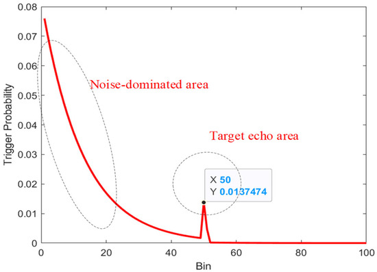
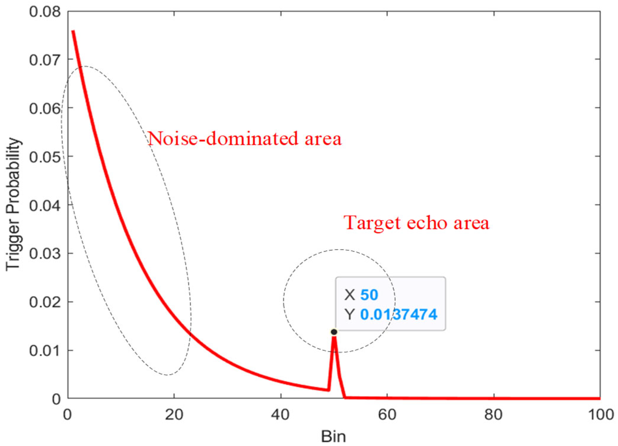
Set the photon number to 0.5203, the noise photon number to 6.50375, the delay of the target echo reaching the detector to 50 bins, the gate width to 100 bins. These parameters are selected to construct a representative low-SBR simulation scenario for analyzing the variation characteristics of the trigger probability curve. Combining with Equation (1), the trigger probability distribution curve of the GM-APD LiDAR echo signal is plotted as shown in Figure 1.

In Figure 1, the horizontal axis represents the time bin index within the gating interval, while the vertical axis represents the trigger probability of the GM-APD detector at each bin. According to the simulation settings, the gating width is 100 bins, and the target echo delay is located at approximately the 50th bin position. Therefore, the region before the target position mainly corresponds to background noise triggering events, while the peak appearing near the target delay position corresponds to the target echo response. The numerical values in the figure indicate the trigger probability magnitude at different bin positions under the simulated low-SBR condition.

The variation rate of the noise interval segment shows a decreasing trend from fast to slow, and there are local peaks in the target interval segment. Furthermore, the first-order difference in the GM-APD echo signal trigger probability is defined as Δn(i) (i = 1, 2, 3, …, N, N ∈ N+), as shown in Equation (3):

$$\Delta n(i)=P(i)-P(i-1) i=1,2\dots ,N,N\in N^{+}$$

(3)

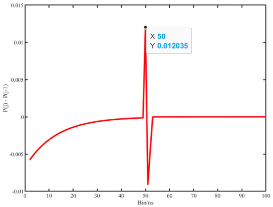
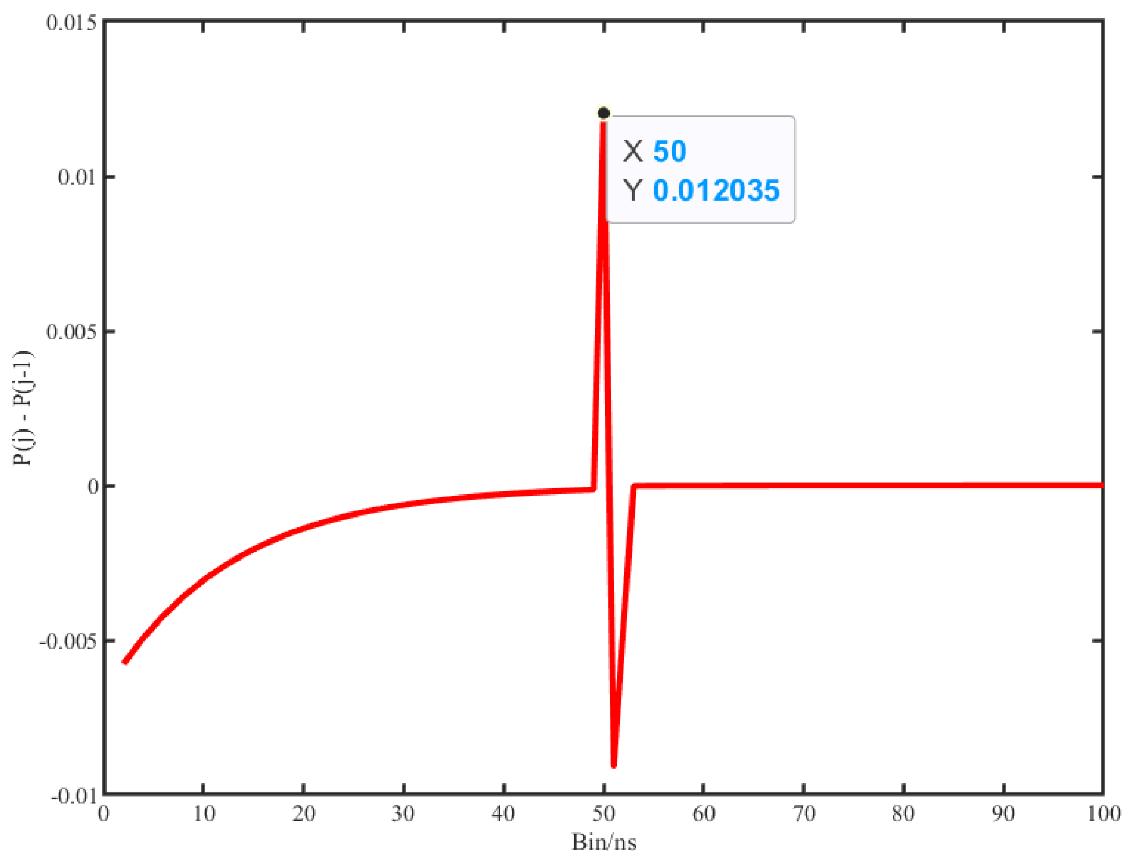
The result of plotting the first-order difference curve of the trigger probability of the GM-APD echo signal is shown in Figure 2:

As can be seen from the above figure, in the first-order difference curve of the trigger probability of the GM-APD echo signal, the first-order difference shows an overall upward trend that is initially fast and then slows down, with a relatively small change range; however, there is a significant amplitude change in the target section.

4. Range Parameter Estimation Method for GM-APD LiDAR Based on Multi-Scale Tracking Differentiator

4.1. Tracking Differentiator Model and Analysis of Parameter Influence

The Tracking Differentiator is a dynamic signal processing tool constructed based on a nonlinear state-space structure. It was originally used for signal tracking and differential estimation in control systems [18].

For the discrete input signal s(k), the tracking differentiator is a discrete-time nonlinear statespace system given by the following:

$$\left\{\begin{array}{l}fh=fhan(s(k),x_1(k),x_2(k),r,h_0)\\ x_1(k+1)=x_1(k)+h{x}_2(k)\\ x_2(k+1)=x_2(k)+h\cdot fh\end{array}\right.$$

(4)

Here, $x_1$(k) represents the tracking state of the input signal, $x_2$(k) represents the estimation of the signal’s rate of change, h is the step size, $h_0$ = mh is the filtering factor, m is the filtering coefficient, fh is the nonlinear adjustment function used to regulate the dynamic response characteristics of the system, r is the tracking factor [19].

The solution equation for the nonlinear regulation function is as follows [20]:

$$\begin{array}{l}fh=-\left\{\begin{array}{l}rsign(a),\left|a\right|>d\\ r{\displaystyle \frac{a}{d}},\left|a\right|\le d\end{array}\right.\\ d=r{h}_0\\ d_0=h_{0}d\\ y(k)=x_1(k)-s(k)+h_0{x}_2(k)\\ a_0=\sqrt{d^2+8r\left|y(k)\right|}\\ a=\left\{\begin{array}{l}{x}_2(k)+{\displaystyle \frac{(a_0-d)}{2}}sign(y(k)),\left|y(k)\right|>d_0\\ \\ x_2(k)+{\displaystyle \frac{y(k)}{h_0}},\left|y(k)\right|\le d_0\end{array}\right.\end{array}$$

(5)

The state-space model in Equations (4) and (5) defines a tracking differentiator that tracks the input signal $s\left(k\right)$ and provides an estimate of its rate of change $x_2\left(k\right)$. Its primary role in this work is to act as a nonlinear dynamic filter that extracts either the overall signal trend or transient features depending on the choice of the tracking factor $r$.

In the tracking differentiator system, the parameter r represents the maximum rate of state change allowed by the control system, thereby determining the trade-off relationship between the dynamic response speed and the filtering characteristics of the system: when r takes a smaller value, the tracking differentiator system has stronger filtering ability but weaker tracking ability; when r takes a larger value, the tracking differentiator system has stronger tracking ability but weaker filtering ability [21].

From the analysis in Section 2, it can be seen that the first-order difference in the trigger probability curve in the background noise interval segment of the GM-APD LiDAR has no abrupt change; however, at the position corresponding to the bin value of the target, the first-order difference in the trigger probability curve has an abrupt change. When r takes a larger value, the system’s response speed to the changes in the input signal is improved, and it can better track the structure of the first-order difference change, obtaining the local features of the target echo; when r takes a smaller value, the system’s restriction on the rate of state change is enhanced, the filtering ability is improved, and it is conducive to suppressing the random disturbance of background noise, and can capture the overall change trend of the trigger probability curve.

4.2. Echo Signal Range Parameter Estimation Method Based on Multi-Scale Tracking Differentiator

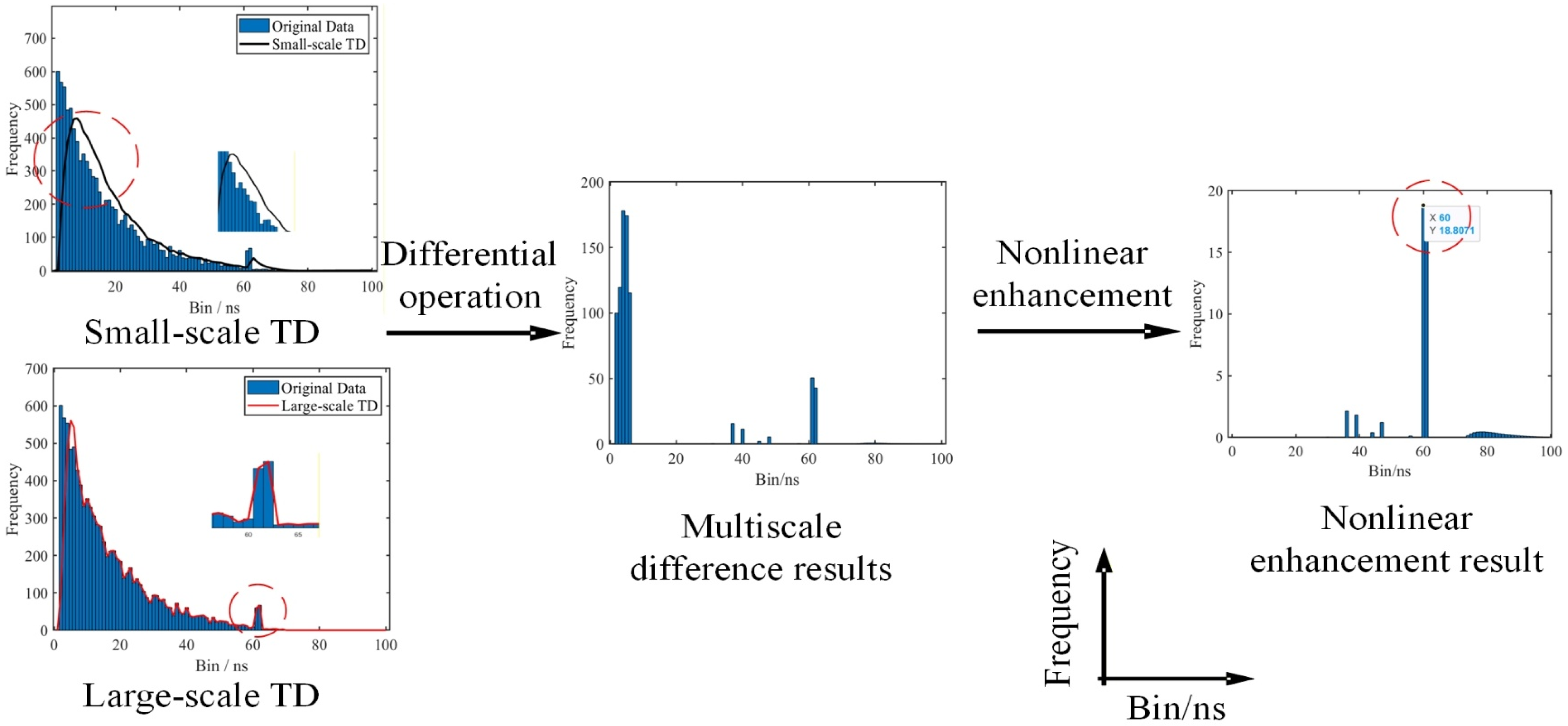
Based on the analysis results in Section 4.1, this section proposes a range parameter estimation method based on multi-scale tracking differentiators. The multi-scale refers to setting different sizes of tracking factors r, constructing tracking outputs with different response capabilities for rate variations, so that the system can characterize the signal from two aspects: the overall trend of the background and the local changes. Using the small-scale r to fit the overall change trend of the echo signal, and the large-scale r to retain the first-order difference jump characteristics of the region where the target echo is located. Further, using the output results of the large-scale and small-scale tracking differentiators to perform a difference to achieve noise suppression. Combined with the statistical characteristics of the photon trigger probability, different weight coefficients are adopted for signals at different positions to perform nonlinear enhancement of the target echo, and finally, the peak threshold method is combined to complete the range parameter estimation.

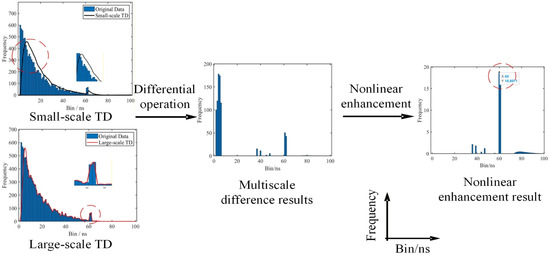
As shown in Figure 3, the proposed framework mainly consists of four stages: dual-scale TD processing, residual signal construction, nonlinear enhancement, and peak extraction. First, the original GM-APD echo signal is processed by both small-scale and large-scale tracking differentiators. The small-scale TD is mainly used to estimate the slowly varying background trend, while the large-scale TD preserves the local abrupt mutation characteristics of the target echo.

Subsequently, the residual signal is obtained by calculating the difference between the outputs of the dual-scale TDs, thereby enhancing the distinguishability between the target echo and background noise. To further suppress front-end residual noise and compensate weak target responses in the rear gating region, a position-dependent nonlinear enhancement operation is introduced. Finally, peak extraction is performed on the enhanced signal to estimate the target range parameter.

In order to ensure that the small-scale tracking results only reflect the overall trend of the signal, the tracking factor r in the tracking differentiator is essentially used to constrain the maximum rate of change in the system state. Therefore, in order to make the small-scale tracking differentiator system only track the overall trend of the signal, its constrained scale should be kept at the same order of magnitude as the amplitude of the noise fluctuation. This paper constructs the small-scale tracking factor $r_s$ using the standard deviation of the global echo data. Calculate the standard deviation of the echo data:

$${\sigma }_{bg}=std(s(1:N))$$

(6)

Here, N represents the width of the gate. This standard deviation characterizes the statistical intensity of the fluctuation of the echo data. The small-scale tracking factor is defined as follows:

$$r_s=l{\sigma }_{bg}$$

(7)

Here, l represents the coverage coefficient, which is an empirical parameter used to appropriately expand the constraint range based on the fluctuation range of the noise amplitude. This is done to ensure that most of the changes in the background noise fall within the nonlinear speed-limiting regulation zone of the tracking differentiator, thereby enabling the system to mainly track the overall trend changes in the signal without generating excessive responses to local abrupt changes.

The trigger frequency histogram s(k) of the GM-APD LiDAR echo signal is processed using the small-scale tracking factor $r_s$:

$$\left\{\begin{array}{l}fh=fhan(s(k),x_1^s(k),x_2^s(k),r_s,h_0)\\ x_1^s(k+1)=x_1^s(k)+h{x}_2^s(k)\\ x_2^s(k+1)=x_2^s(k)+h\cdot fh\end{array}\right.$$

(8)

The nonlinear function fh is solved as shown in Equation (5), from which the output $x_1^s$(k) representing the overall signal trend is obtained.

To ensure that the large-scale tracking differentiator system can completely preserve the target echo structure, the upper bound of the constraints should cover the first-order difference variation range of the target signal. The large-scale tracking factor is defined as follows:

$$r_b=n{r}_s$$

(9)

Here, n is the scale expansion coefficient, which is selected based on experience. Its function is to expand the maximum allowable rate of change range of the system, enabling the tracking differentiator system to maintain the abrupt structure of the target echo.

The trigger frequency histogram of the GM-APD LiDAR echo signal is processed using the large-scale tracking factor $r_b$:

$$\left\{\begin{array}{l}fh=fhan(s(k),x_1^b(k),x_2^b(k),r_b,h_0)\\ x_1^b(k+1)=x_1^b(k)+h{x}_2^b(k)\\ x_2^b(k+1)=x_2^b(k)+h·fh\end{array}\right.$$

(10)

The nonlinear function fh is solved as shown in Equation (5), from which the precise rate of change in the echo data for tracking output $x_1^b(\mathrm{k})$ is obtained.

Next, a residual signal is constructed by performing a differential operation on the outputs of the large-scale and small-scale tracking differentiator systems:

$$I(k)=x_1^b(k)-x_1^s(k)$$

(11)

And truncate the negative values to suppress non-physical residuals:

$$I^{\prime }(k)=\max \left\{I(k),0\right\}$$

(12)

After completing the differential operation of the output of the large-scale and small-scale tracking differentiator system, although most of the background noise has been effectively suppressed, there are still certain residual signals in the front-end region before the gating. This residual mainly comes from two factors: Firstly, the GM-APD laser radar adopts a first-photon triggering detection mechanism. When noise photons arrive before the target echo, a phenomenon of photon front accumulation occurs. Secondly, as a nonlinear system with dynamic adjustment characteristics, the output of the tracking differentiator inevitably has a certain phase delay when tracking the input changes. The system output is difficult to completely synchronize with the input changes, thus manifesting as the residual response in the front-end region before the gating in the differential result. To further suppress the residual noise at the front-end, it is necessary to first analyze the variation law of the triggering probability of the target signals at each position within the gating.

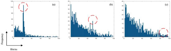
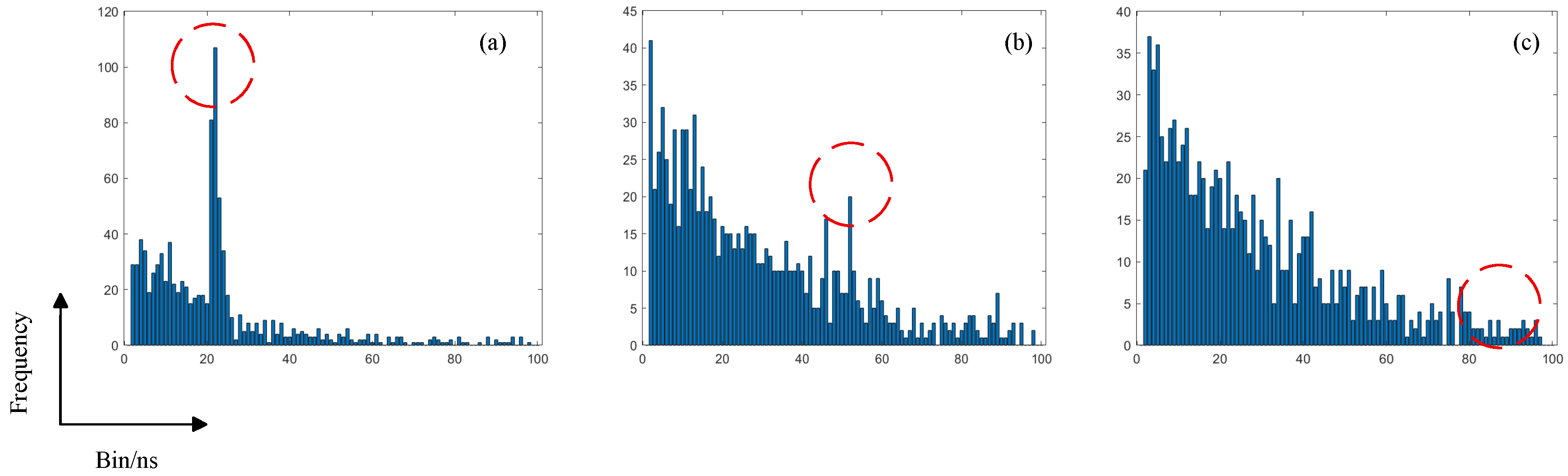
Set the SBR to 0.08 and the frame number to 1000. The target positions are respectively at 20 bins, 50 bins, and 90 bins, they respectively represent the front end, middle end and rear end of the select gate. The simulation results are shown in Figure 4. It can be seen that as the target position moves towards the end of the gate, the target triggering frequency shows an overall decreasing trend with the bin position.

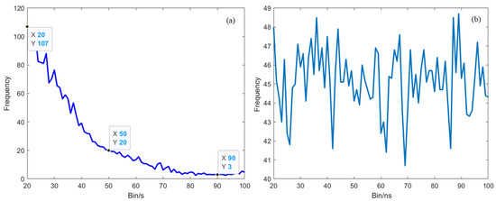
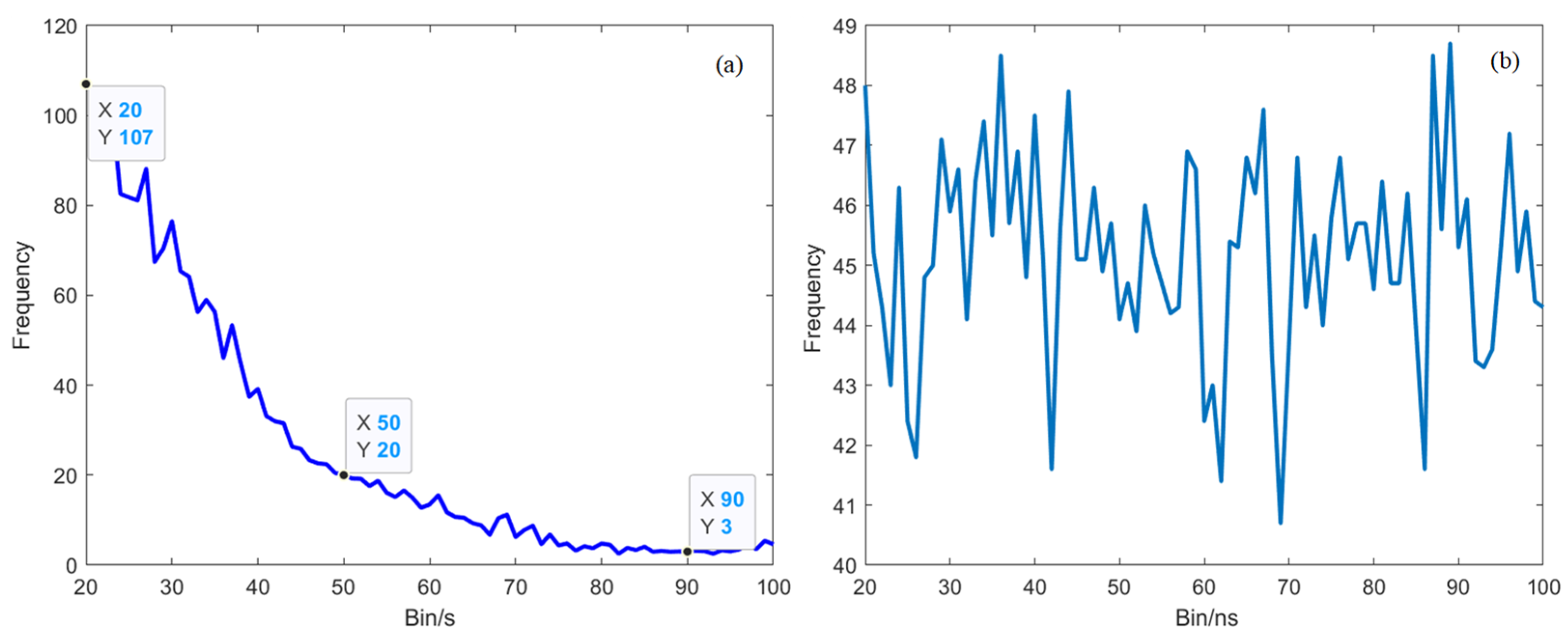
Set the first 19 bins as the pure noise area, and set the target signal to be from bin 20 to bin 100. Keep the SBR constant at 0.08. Simulate the target peak trigger frequency when the target is at each position within a distance of 20 bins to 100 bins. The results are shown in Figure 5a, and it can be seen that the curve shows an overall decreasing trend, verifying the conclusion that the target trigger peak frequency gradually decreases with the bin position as a whole. Use the first 19 bins as the estimation interval for the pure background noise without targets. Simulate the average noise trigger frequency of the first 19 bins when the target position changes from bin 20 to bin 100. The results are shown in Figure 5b, and it can be seen that within the gate, the trigger frequency of the noise randomly changes within a limited range.

Therefore, it can be concluded that in the front-end area of the gate, the target peak frequency is relatively high, and the SBR is also relatively high; while in the rear-end area of the gate, the target peak is smaller, and the SBR is relatively low.

To enhance the range information of the target after the differential signal processing, this paper introduces a nonlinear enhancement strategy. This method constructs a position-dependent weight function based on the time bin position and performs nonlinear weighting on the differential signal.

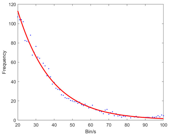
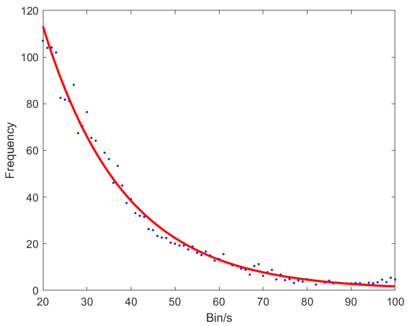
Perform a least squares fit on Figure 5a, and the result is shown in Figure 6:

This is a form of exponential decay, so our nonlinear enhancement function should be an exponential function. In the front-end region before the gating, a smaller weight is assigned to suppress the residual data in the high-confidence area; while in the rear-end region after the gating, the weight gradually increases to compensate for the target peak attenuation caused by the noise accumulation effect, thereby improving the detectability of distant weak targets.

Construct the weight function w(k):

$$w(k)=\left\{\begin{array}{ll}\alpha {({\displaystyle \frac{k}{N}})}^3& {\mathrm{T}}_n\le \mathrm{k}<\mathrm{N}\\ 0& { 0<\mathrm{k}<\mathrm{T}}_n\end{array}\right.$$

(13)

Here, k represents the position of the data time bin value, $N$ is the selectivity gate width, and is the enhancement intensity. The selection of $T_n$ is highly relevant to the target scenario. On the one hand, an appropriate value can be given based on system design parameters or task requirements (such as measurement range), or it can be determined during system calibration and correction based on the strong prior information of the known scene. Non-linear enhancement is performed on the output of multi-scale TD, $I^{\prime }(k)$:

$$L(k)=I^{\prime }(k)·w(k)$$

(14)

Obtaining $L(k)$ represents the histogram of the trigger frequency of the nonlinearly enhanced GM-APD LiDAR. Through the aforementioned nonlinear enhancement strategy, it is possible to suppress the residual response at the front end of the gating process while effectively compensating for weak targets at the rear end, thereby enhancing the stability and robustness of the overall target detection.

Finally, the peak threshold method is used to process the nonlinearly enhanced trigger frequency histogram [22], and the target range is as follows:

$$pos=\arg {\max }_{pos}[L(k)]$$

(15)

Here, $pos$ represents the information about the signal echo range.

The pseudo-code of the method in this article is Algorithm 1 as follows:

Algorithm 1. Multi-Scale Tracking Differentiator-Based Range Parameter Estimation

Input: Photon-count histogram: s(k); 1: Initialize: n, h, l, $T_n$ 2: Compute background noise standard deviation: ${\sigma }_{bg}=std(s(1:T_n))$ 3: Determine small-scale tracking factor: $r_s=l{\sigma }_{bg}$ 4: Compute TD function: $\left\{\begin{array}{l}fh=fhan(s(k),x_1^s(k),x_2^s(k),r_s,h_0)\\ x_1^s(k+1)=x_1^s(k)+h{x}_2^s(k)\\ x_2^s(k+1)=x_2^s(k)+h\cdot fh\end{array}\right.$ 5: Determine large-scale tracking factor: $r_b=n{r}_s$ 6: Compute TD function: $\left\{\begin{array}{l}fh=fhan(s(k),x_1^b(k),x_2^b(k),r_b,h_0)\\ x_1^b(k+1)=x_1^b(k)+h{x}_2^b(k)\\ x_2^b(k+1)=x_2^b(k)+h·fh\end{array}\right.$ 7: Construct difference signal: $I(k)=x_b(k)-x_s(k)$, $I^{\prime }(k)=\max \left\{I(k),0\right\}$ 8: Perform nonlinear enhancement: $L(k)=I^{\prime }(k)·w(k)$ Output: Estimated range position (pos)

5. Experimental Verification and Result Analysis

5.1. Evaluation Index

To verify the effectiveness of the range parameter estimation algorithm proposed in this paper, simulation methods were employed to evaluate and analyze the performance of the algorithm. The evaluation indicators used in this paper include root mean square error (RMSE) [23], Restoration Degree (RD), and Variance (Var) [24].

5.2. Simulation Experiments and Result Analysis

All simulations and data processing in this work were implemented in MATLAB R2024a on a personal computer equipped with an Intel Core i7 processor, 16 GB RAM, and an NVIDIA GeForce RTX-series GPU.

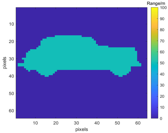
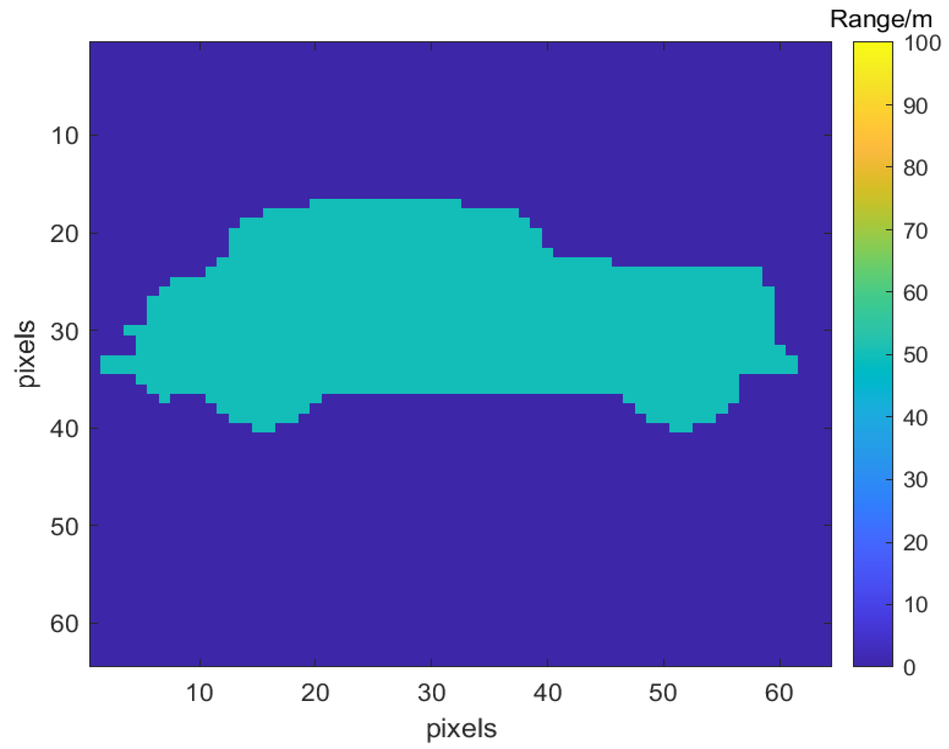
This paper adopts the Monte Carlo data simulation method from reference [25] and sets the car at a range of 50 m as the reference range image, as shown in Figure 7.

Obtain the simulation data of GM-APD LiDAR with different SBR. The simulation parameters are set as shown in

Table 1. Key parameters of the GM-APD LiDAR echo signal simulation.

No.	Parameter	Value
1	PPP	0.1041
2	SBR	0.08, 0.07, 0.06, 0.05, 0.04, 0.03
3	Pixel number	64 × 64
4	Bin width	1 ns
5	Delay	280 ns
6	Gate width	100 ns
7	Target location	Car (50 m)
8	Monte Carlo experiment repetitions	1000

. In particular, in this paper, the gate delay is set to 280 ns and the gate width is set to 100 ns to ensure that the target is within the gate interval.

5.2.1. Algorithm Robustness Experiment

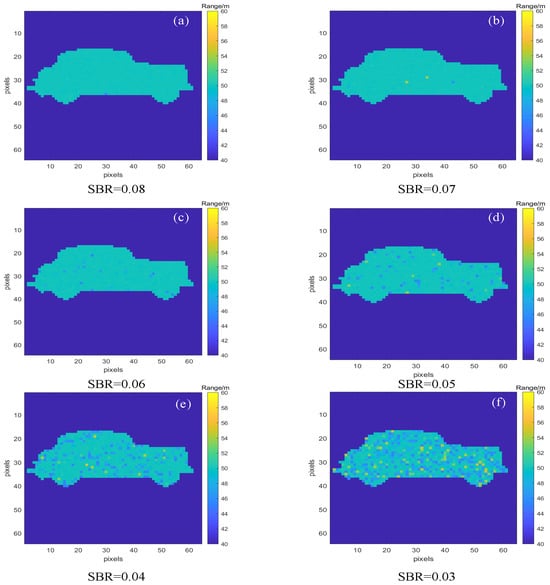
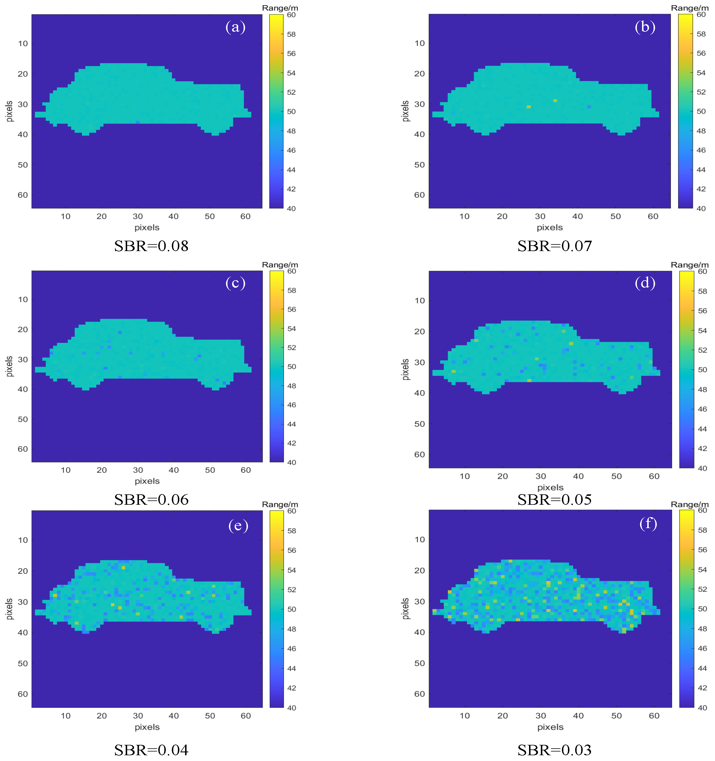
In order to verify the robustness of the algorithm proposed in this paper under different signal-to-interference ratios, data processing was carried out using the method presented in this paper under various SBRs. The results are shown in Figure 8.

As can be seen from Figure 8, as the SBR increases, the method adopted in this paper can generate a clearer edge structure of the range image and reduce the range of abnormal noise. When the SBR is as low as 0.04, the method proposed in this paper still shows good performance, being able to restore most of the range information with fewer noise points. To further evaluate the robustness of the method proposed in this paper, RMSE, RD and Var are used as objective quantitative indicators to evaluate the processing results of the method proposed in this paper as shown in

Table 2. Quantitative evaluation results of different SBRs.

SBR	0.08	0.07	0.06	0.05	0.04	0.03
RMSE	0.1607	0.2585	0.8122	1.1173	1.4779	2.0705
RD	0.9989	0.9957	0.9786	0.9282	0.8124	0.5916
Var	3.1675 × 10−7	2.4453 × 10−7	8.6963 × 10−7	7.9671 × 10−6	1.4947 × 10−6	7.6651 × 10−5

.

As shown in Table 2, when the SBR is greater than or equal to 0.04, the RD after processing by the method proposed in this paper is greater than 0.8124, the RMSE is less than 1.4779, and the fluctuation range of the evaluation indicators is small, indicating that the method proposed in this paper is robust when the SBR is greater than or equal to 0.04. In addition, when the SBR is greater than or equal to 0.04, the Var of the method proposed in this paper in 1000 Monte Carlo experiments is less than 1.4947 × 10⁻⁶, indicating that the method proposed in this paper has stable range parameter estimation ability.

5.2.2. Algorithm Superiority Experiment

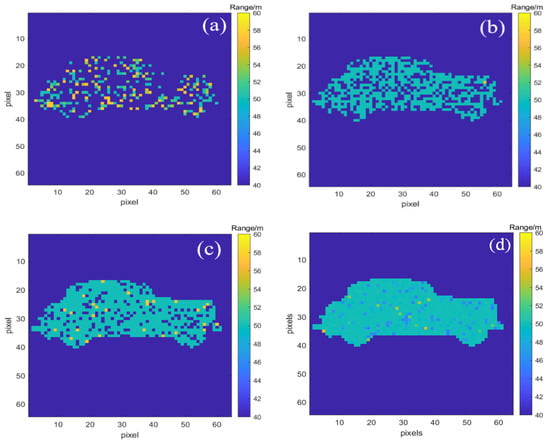
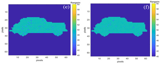
In order to verify the superiority of the algorithm, with a fixed SBR = 0.06, the peak method (Peak), maximum likelihood estimation (MLE), kernel density estimation (KDE), Shi’s method, and Chi’s method were used as comparison methods. The processing results are shown in Figure 9.

As can be seen from Figure 9, the range image processed by the method proposed in this paper has a complete structure, the target is basically fully restored, and there is basically no noise. However, the range values of the range image processed by the Peak method are incorrect, and the range images processed by the MLE and KDE methods also have a lot of abnormal range noises. Further quantitative evaluation of the processing results of each algorithm is shown in

Table 3. Quantitative evaluation results of different algorithms.

Method	Peak	MLE	KDE	Shi [14]	Chi [12]	Proposed
RMSE	9.7130	8.4170	1.3175	1.4753	1.0007	0.8122
RD	0.2615	0.6302	0.8156	0.8672	0.9184	0.9786
Var	7.2675 × 10−5	2.4453 × 10−6	6.5714 × 10−6	4.2441 × 10−6	1.8867 × 10−6	8.6963 × 10−7

.

Compared with the conventional method, the proposed method reduces the RMSE by at least 38.35%, increases the RD by at least 19.99%, and simultaneously increases the variance by at least one order of magnitude. This verifies the superiority of the method presented in this paper.

5.3. GM-APD LiDAR Field Acquisition Experiment Verification and Result Analysis

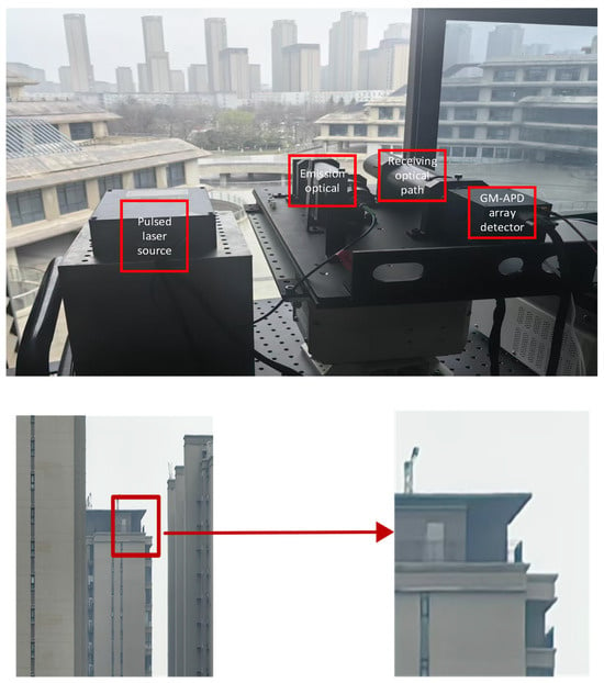
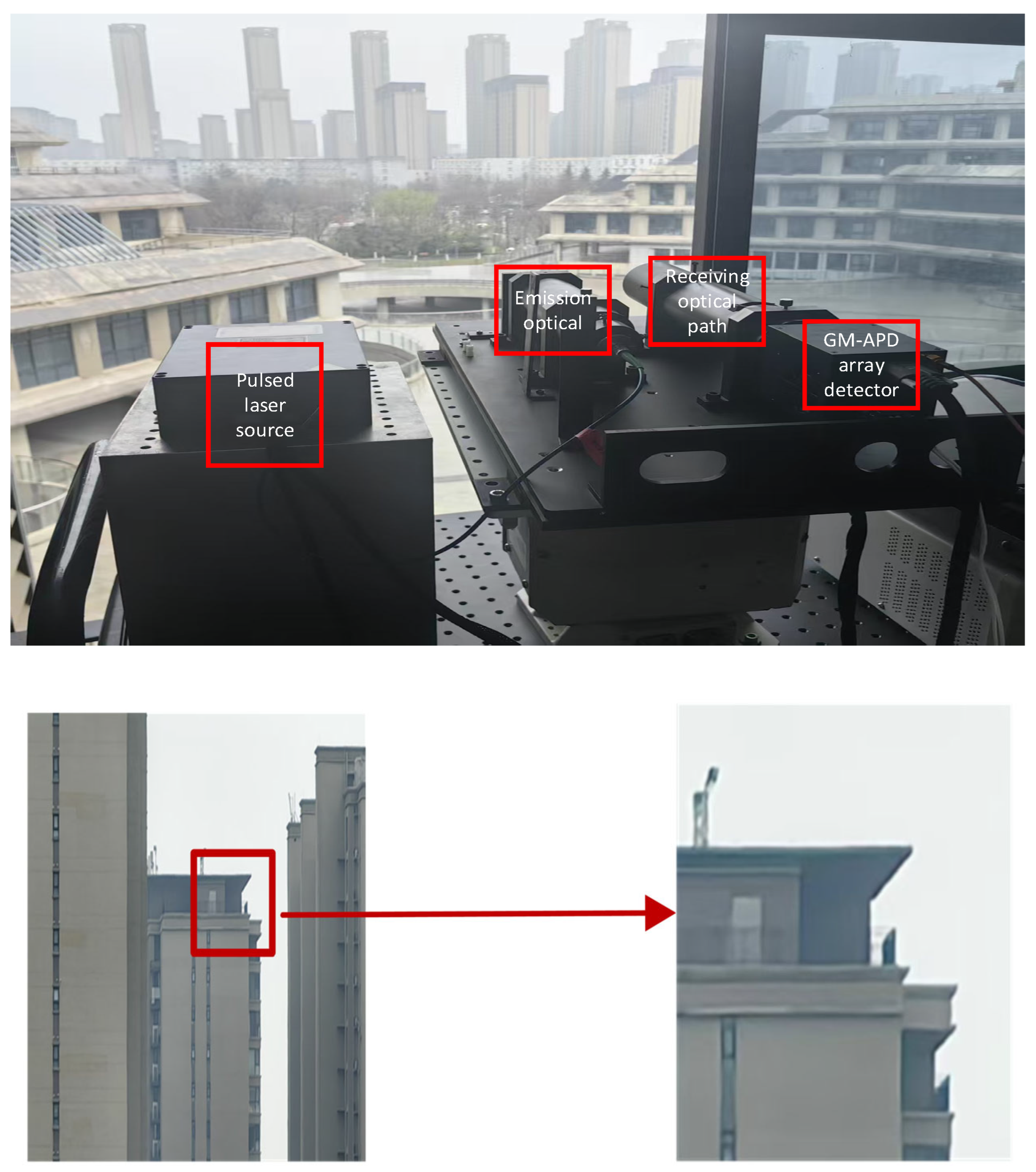
The proposed algorithm was verified through practical experimental tests. The laser radar system used in this experiment was a 64 × 64 transceiver-separated GM-APD laser radar, as shown in Figure 10. The building targets 830–860 m away were detected and imaged under clear outdoor weather conditions.

The key parameters in this detection scenario are shown in

Table 4. Key parameters of GM-APD LiDAR detection and imaging.

No.	Parameter	Value
1	PPP	0.13
2	SBR	0.038
3	Pixel number	64 × 64
4	Bin width	1 ns
5	Delay	5 ns
6	Laser single pulse energy	100 μJ
7	Target location	Building (830–860 m)

. Here, PPP and SBR are calculated according to the method provided in reference [26].

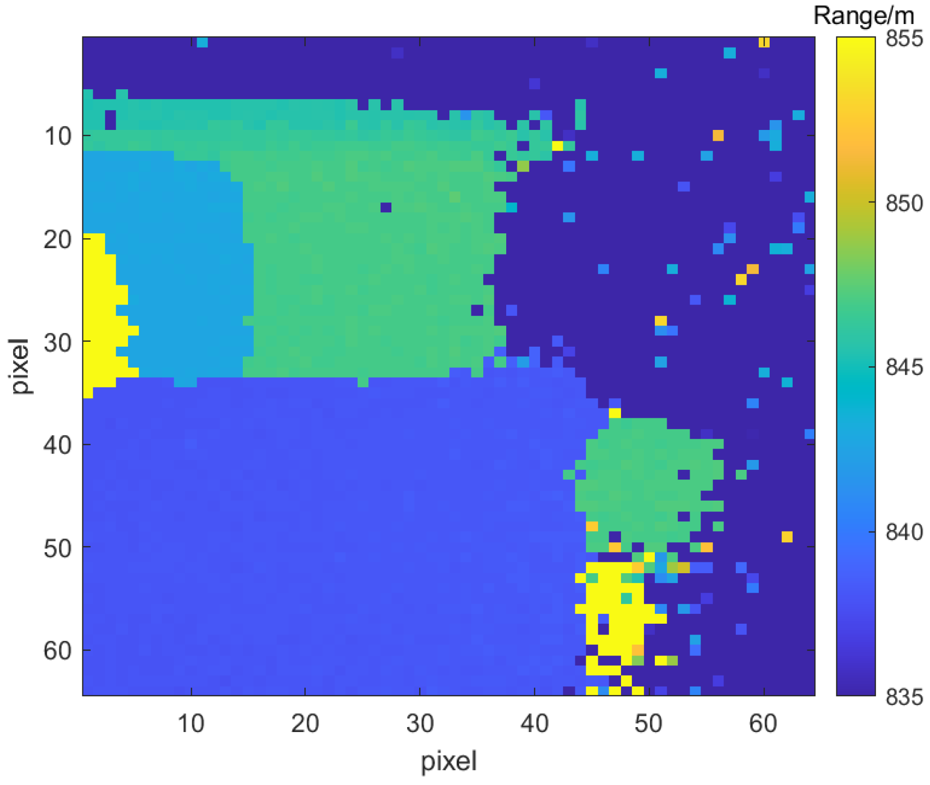
In order to further evaluate the algorithm performance of the method proposed in this paper in the real data collection scenario, data without background noise at night was obtained in the same scenario, and this data was processed using the algorithm proposed in this paper. It was used as the reference image as shown in Figure 11.

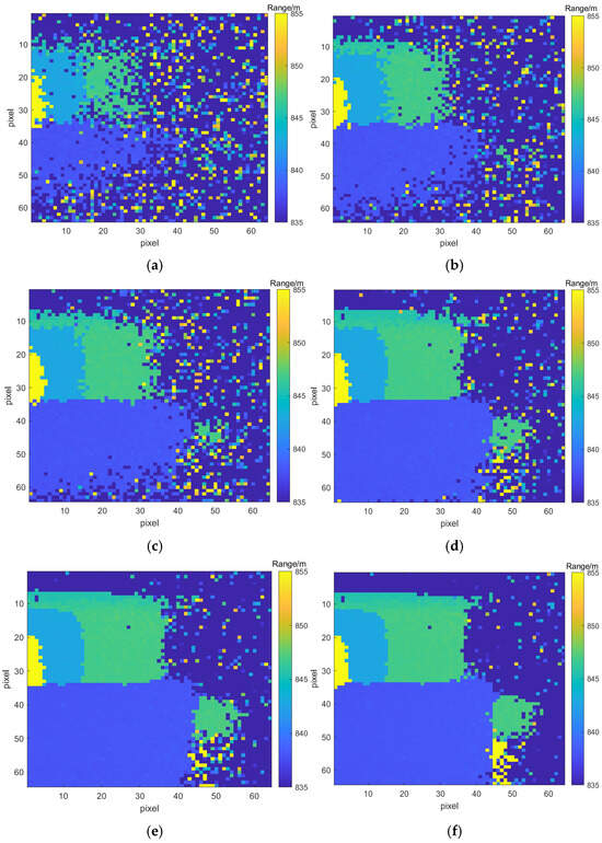
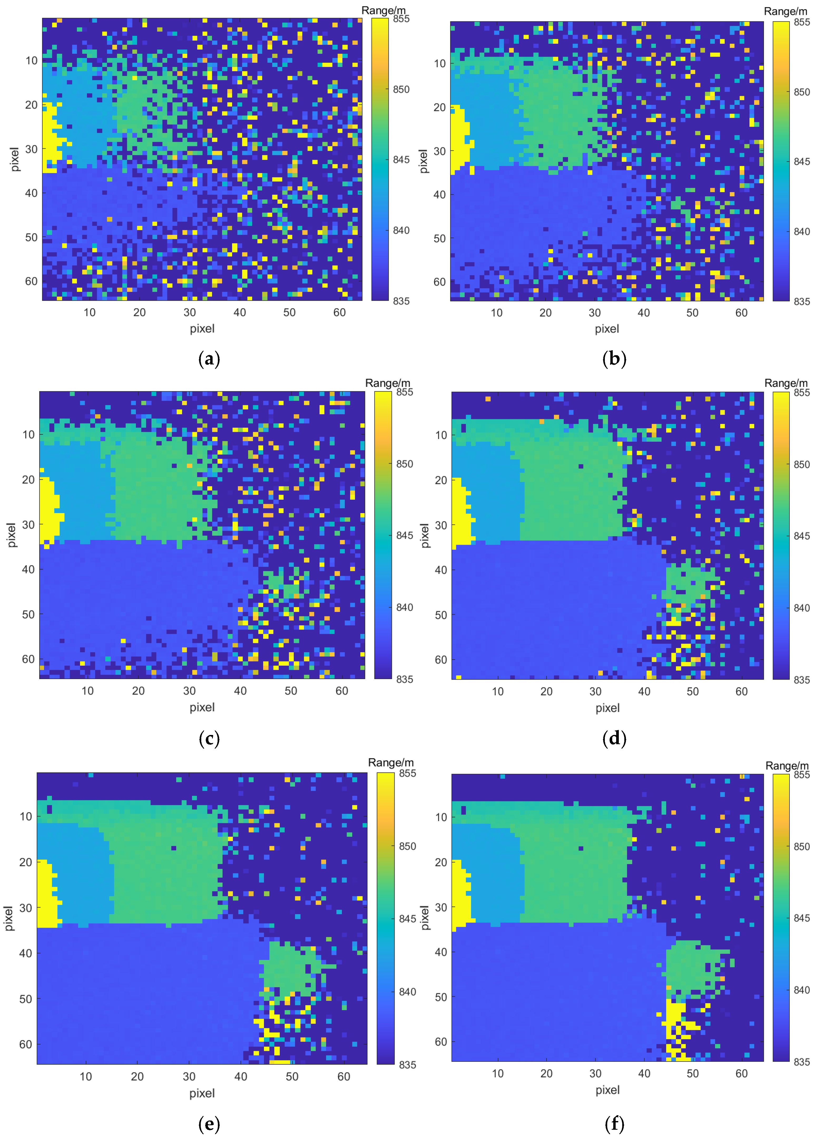
In order to verify the superiority of the algorithm proposed in this paper and to compare the results processed by this algorithm with those processed by Peak, MLE and KDE algorithms, Shi’s method, Chi’s method, the processing results are shown in Figure 12.

As shown in Figure 12, the target range images obtained based on Peak and MLE are missing some target information, and the obtained range images contain a large amount of noise; the target range images obtained based on KDE can obtain most of the target information, but there is a phenomenon of missing the details and contours of the target edges; the target range images obtained by the algorithm proposed in this paper have better target edge detail contours and fewer noise points.

The proposed method in this paper was evaluated using RMSE, RD, and Var for quantitative assessment. The results are shown in

Table 5. Quantitative evaluation results of different algorithms in the real-world experiment.

Method	Peak	MLE	KDE	Shi [14]	Chi [12]	Proposed
RMSE	20.1130	6.8658	3.8823	3.0565	2.9717	2.3941
RD	0.1801	0.5033	0.7859	0.8321	0.8867	0.9182
Var	2.0068 × 10−4	2.3661 × 10−6	8.9875 × 10−6	4.7481 × 10−6	2.8867 × 10−6	1.0240 × 10−7

.

As shown in Table 5, the range parameter estimation method based on the multi-scale tracking differentiator obtained the highest range image RD, and the RMSE and Var were the lowest. Compared with the comparison algorithm, RD was at least improved by 16.83%, and RMSE was at least reduced by 38.34%, which verified the effectiveness and superiority of the algorithm proposed in this paper.

6. Discussion

The experimental and simulation results presented in this study demonstrate that the proposed multi-scale tracking differentiator (TD) method achieves superior range parameter estimation performance compared with conventional approaches such as Peak, MLE, and KDE. The method effectively suppresses noise while preserving weak transient target features, leading to a higher restoration degree (RD) and lower RMSE and variance under extremely low SBR conditions. These results confirm that the multi-scale TD approach is particularly suitable for single-photon LiDAR systems operating in harsh noise environments where traditional statistical or spatial-prior-based methods may fail.

Compared with recent deep learning–based methods for LiDAR signal denoising and range estimation, the proposed method has several distinctive advantages. Unlike neural network approaches that require large labeled datasets for training and may suffer from generalization issues in unseen environments, the multi-scale TD method is model-free and does not rely on prior training data. It provides real-time signal processing with deterministic behavior, making it more interpretable and robust in scenarios with extremely low SBR or rare events. On the other hand, deep learning methods may offer better adaptability to complex and highly dynamic scenes when sufficient data is available, especially in multi-target or cluttered environments. Therefore, while deep learning techniques represent a promising direction for highly adaptive LiDAR processing, the proposed method offers a complementary solution that ensures reliable performance under conditions where training data is scarce or noise dominates.

However, some limitations should be noted. The performance of the method depends on the appropriate selection of tracking factors (r) for both small-scale and large-scale differentiators, which are currently determined based on empirical or prior system knowledge. In dynamic scenarios where the background noise characteristics or target reflectivity vary rapidly, the fixed parameters may not fully capture the optimal filtering-tracking trade-off, potentially leading to slight degradation in estimation accuracy. Additionally, the nonlinear enhancement strategy, while effective in compensating for distant weak targets, may require careful tuning of the weight function parameters for different range distributions and target densities.

Future work could focus on adaptive parameter selection, where tracking factors and enhancement coefficients are dynamically adjusted based on real-time signal statistics. Integration of scene-adaptive, learning-based, or hybrid methods may further improve robustness in complex environments. Moreover, the extension of this approach to multi-target or multi-layer echo scenarios, as well as integration with 3D reconstruction pipelines, would be valuable for practical single-photon LiDAR applications in autonomous driving, remote sensing, and long-range target detection.

In summary, the proposed method provides a model-free, nonlinear signal processing solution that balances noise suppression and target preservation, offering a promising direction for robust, high-fidelity range estimation in low SBR single-photon LiDAR systems, and serves as a complementary alternative to data-driven approaches in challenging scenarios.

7. Conclusions

This paper addresses the challenges faced by GM-APD LiDAR in low SBR conditions, such as the degradation of range parameter estimation performance and the difficulty in three-dimensional target reconstruction. To overcome these issues, a range parameter estimation method based on a multi-scale tracking differentiator is proposed. This method effectively avoids strong dependence on explicit probabilistic inference models and spatial prior assumptions. It achieves precise extraction and reconstruction of target information through a nonlinear dynamic tracking mechanism. The research results show that the proposed method demonstrates significant superiority and robustness in both simulation and actual collected data. In simulation experiments, when the SBR is as low as 0.04, the proposed method still maintains high target restoration and low root mean square error, proving its robustness in extremely weak signal environments. Compared with typical methods such as Peak, MLE, and KDE, the proposed method maintains a complete range image structure, fully restores the target, and has very few noise points when the fixed SBR is 0.06. Quantitative evaluation shows that compared with the comparison algorithms, the RMSE is at least reduced by 38.35%, the RD is at least increased by 19.99%, and the variance is at least increased by one order of magnitude. This demonstrates that the proposed method achieves improved range estimation accuracy and stability under low-SBR conditions. In the real data test of building targets ranging from 830 m to 860 m, the range images obtained by the proposed method have better target edge contour details and far fewer noise points than the Peak, MLE, and KDE methods. This study provides an efficient and reliable solution through an unmodel-based, nonlinear signal processing approach for achieving high-fidelity single-photon three-dimensional imaging and target detection under harsh low SBR conditions. It alleviates the dependence of traditional methods on probabilistic distribution assumptions and spatial prior constraints, and opens up a new technical path for high-reliability range perception and three-dimensional target reconstruction of single-photon LiDAR in strong background noise environments.

Nevertheless, several limitations still exist in the proposed framework. First, the current method is mainly validated on static target scenes, while the performance under dynamic target conditions has not yet been fully investigated. Target motion may introduce temporal spreading and range migration effects, which could influence the stability of the trigger probability distribution and the tracking performance of the multi-scale TD framework. Second, some parameters in the proposed method are currently selected empirically, and adaptive parameter optimization for different imaging scenarios requires further study. In addition, under extremely weak echo conditions where the target signal is heavily submerged in background noise, the local mutation characteristics of the trigger probability curve may become less distinguishable, which could affect target extraction performance.

This paper primarily focuses on the proposed multi-scale tracking differentiator method for range parameter estimation under low SBR conditions on static targets. Experiments involving dynamic target and adaptive parameter optimization in rapidly changing noise environments are not included in this work and are planned for future study. The current results establish a foundation for those subsequent investigations.

References

- Achilles, D.; Silberhorn, C.; Śliwa, C.; Banaszek, K.; Walmsley, I.A. Fiber-assisted detection with photon number resolution. Opt. Lett. 2003, 28, 2387–2389. [Google Scholar] [CrossRef] [Scilit] [PubMed]
- Saito, Y.; Kurata, H.; Kurushima, H.; Kobayashi, F.; Kawahara, T.D.; Nomura, A.; Maruyama, T.; Tanaka, M. Experimental discussion on eye-safe 1.54 μm photon counting LiDAR using avalanche photodiode. Opt. Rev. 2004, 11, 378–384. [Google Scholar] [CrossRef] [Scilit]
- Wang, Y.; Wei, X.; Wang, C.; Liu, X.; Xie, D.; Yuan, K.; Li, R. A non-local regularization-based fractional-order total variational compressive sensing algorithm for effective recovery of Geiger-mode avalanche photodiode LiDAR images. AIP Adv. 2025, 15, 015102. [Google Scholar]
- Dai, J.; Li, S.; Gao, F.; Cao, H.; Guo, G.; Liu, X.; Wang, Q. Performance analysis of the photon-counting LiDAR based on the statistical property. In Signal and Information Processing, Networking and Computers: Proceedings of the 8th International Conference on Signal and Information Processing, Networking and Computers (ICSINC); Springer Nature: Singapore, 2022; pp. 534–541. [Google Scholar]
- Liu, D.; Sun, J.F.; Lu, W.; Li, S.; Zhou, X. 3D reconstruction of the dynamic scene with high-speed targets for GM-APD LiDAR. Opt. Laser Technol. 2023, 161, 109114. [Google Scholar] [CrossRef] [Scilit]
- Aloni, D.; Stern, A.; Javidi, B. Three-dimensional photon counting integral imaging reconstruction using penalized maximum likelihood expectation maximization. Opt. Express 2011, 19, 19681–19687. [Google Scholar] [CrossRef] [Scilit] [PubMed]
- Halimi, A.; Maccarone, A.; Lamb, R.A.; Buller, G.S.; McLaughlin, S. Robust and guided bayesian reconstruction of single-photon 3D LiDAR data: Application to multispectral and underwater imaging. IEEE Trans. Comput. Imaging 2021, 7, 961–974. [Google Scholar] [CrossRef] [Scilit]
- Rapp, J.; Goyal, V.K. A few photons among many: Unmixing signal and noise for photon-efficient active imaging. IEEE Trans. Comput. Imaging 2017, 3, 445–459. [Google Scholar] [CrossRef] [Scilit]
- Ma, L.; Sun, J.; Liu, D.; Zhou, X. Noise-suppression algorithm of GM-APD LiDAR based on Markov random field. Opt. Laser Technol. 2023, 169, 110026. [Google Scholar]
- Chen, S.; Halimi, A.; Ren, X.; McCarthy, A.; Su, X.; McLaughlin, S.; Buller, G.S. Learning non-local spatial correlations to restore sparse 3D single-photon data. IEEE Trans. Image Process. 2019, 29, 3119–3131. [Google Scholar]
- Halimi, A.; Ciuciu, P.; McCarthy, A.; McLaughlin, S.; Buller, G.S. Fast adaptive scene sampling for single-photon 3D lidar images. In Proceedings of the 2019 IEEE 8th International Workshop on Computational Advances in Multi-Sensor Adaptive Processing (CAMSAP), Le Gosier, Guadeloupe, 15–18 December 2019. [Google Scholar]
- Chi, K.H.; Liu, X.L.; Kong, W.; Xue, R.; Huang, G. Few-photon pixel-level target detection imaging based on 64×64 array GM-APD LiDAR system. Infrared Phys. Technol. 2025, 135, 105722. [Google Scholar]
- Lu, Y.; He, W.J.; Wu, M. Time-correlated Kalman depth estimation for photon-counting LiDAR. Acta Photon. Sin. 2021, 50, 0311001. [Google Scholar]
- Shi, Z.; Sun, J.; Cui, D.; Zhou, X.; Ni, H. GM-APD LiDAR reconstruction algorithm with few frames based on sample function. Opt. Laser Technol. 2025, 192, 113866. [Google Scholar] [CrossRef] [Scilit]
- Altmann, Y.; Ren, X.; McCarthy, A.; Buller, G.S.; McLaughlin, S. Lidar waveform-based analysis of depth images constructed using sparse single-photon data. IEEE Trans. Image Process. 2016, 25, 1935–1946. [Google Scholar] [CrossRef] [Scilit] [PubMed]
- Kirmani, A.; Venkatraman, D.; Shin, D.; Colaço, A.; Wong, F.N.C.; Shapiro, J.H.; Goyal, V.K. First-photon imaging. Science 2014, 343, 58–61. [Google Scholar] [CrossRef] [Scilit] [PubMed]
- Zhang, Y.; Li, S.; Sun, J.; Zhang, X.; Zhou, X.; Zhang, H. Noise-tolerant depth image estimation for array Gm-APD LiDAR through atmospheric obscurants. Opt. Laser Technol. 2024, 175, 110706. [Google Scholar]
- Wang, X.; Yau, S.; Huang, J. A study of tracking-differentiator. In Proceedings of the 39th IEEE Conference on Decision and Control, Sydney, Australia, 12–15 December 2000; pp. 4783–4784. [Google Scholar]
- Liu, X.L.; Li, X.M.; Xiao, B.; Wang, C.; Ma, B. LFM signal parameter estimation via FTD-FRFT in impulse noise. Fractal Fract. 2023, 7, 69. [Google Scholar] [CrossRef] [Scilit]
- Wang, Z.; Long, Z.; Xie, Y.; Ding, J.; Luo, J.; Li, X. A discrete nonlinear tracking-differentiator and its application in vibration suppression of maglev system. Math. Probl. Eng. 2020, 2020, 1849816. [Google Scholar] [CrossRef] [Scilit]
- Abdul-Adheem, W.R.; Ibraheem, I.K.; Humaidi, A.J.; Alkhayyat, A.; Maher, R.A.; Abdulkareem, A.I.; Azar, A.T. Design and analysis of a novel generalized continuous tracking differentiator. Ain Shams Eng. J. 2022, 13, 101656. [Google Scholar] [CrossRef] [Scilit]
- Shin, D.; Kirmani, A.; Goyal, V.K.; Shapiro, J.H. Photon-efficient computational 3-D and reflectivity imaging with single-photon detectors. IEEE Trans. Comput. Imaging 2015, 1, 112–125. [Google Scholar] [CrossRef] [Scilit]
- Chi, K.; Liu, X.; Xue, R.; Huang, G. SP-LiDAR for fast and robust depth imaging at low SBR and few photons. Photonics 2025, 12, 1229. [Google Scholar] [CrossRef] [Scilit]
- Wei, X.; Wang, C.; Li, R.; Xie, D.; Liu, X.; Yuan, K. Range image reconstruction from GM-APD LiDAR data based on Neyman-Pearson criterion. IEEE J. Sel. Top. Appl. Earth Obs. Remote Sens. 2026, 19, 4301–4318. [Google Scholar] [CrossRef] [Scilit]
- Lindell, D.B.; O’Toole, M.; Wetzstein, G. Single-photon 3D imaging with deep sensor fusion. ACM Trans. Graph. 2018, 37, 113. [Google Scholar] [CrossRef] [Scilit]
- O’Brien, M.E.; Fouche, D.G. Simulation of 3D laser radar systems. Linc. Lab. J. 2005, 15, 37–60. [Google Scholar]
Disclaimer/Publisher’s Note: The statements, opinions and data contained in all publications are solely those of the individual author(s) and contributor(s) and not of MDPI and/or the editor(s). MDPI and/or the editor(s) disclaim responsibility for any injury to people or property resulting from any ideas, methods, instructions or products referred to in the content. |
© 2026 by the authors. Licensee MDPI, Basel, Switzerland. This article is an open access article distributed under the terms and conditions of the Creative Commons Attribution (CC BY) license.