

RASC: Region-Aware Self-Calibration for Dense 2D Sensor Arrays
Abstract
1. Introduction
1.1. Contribution
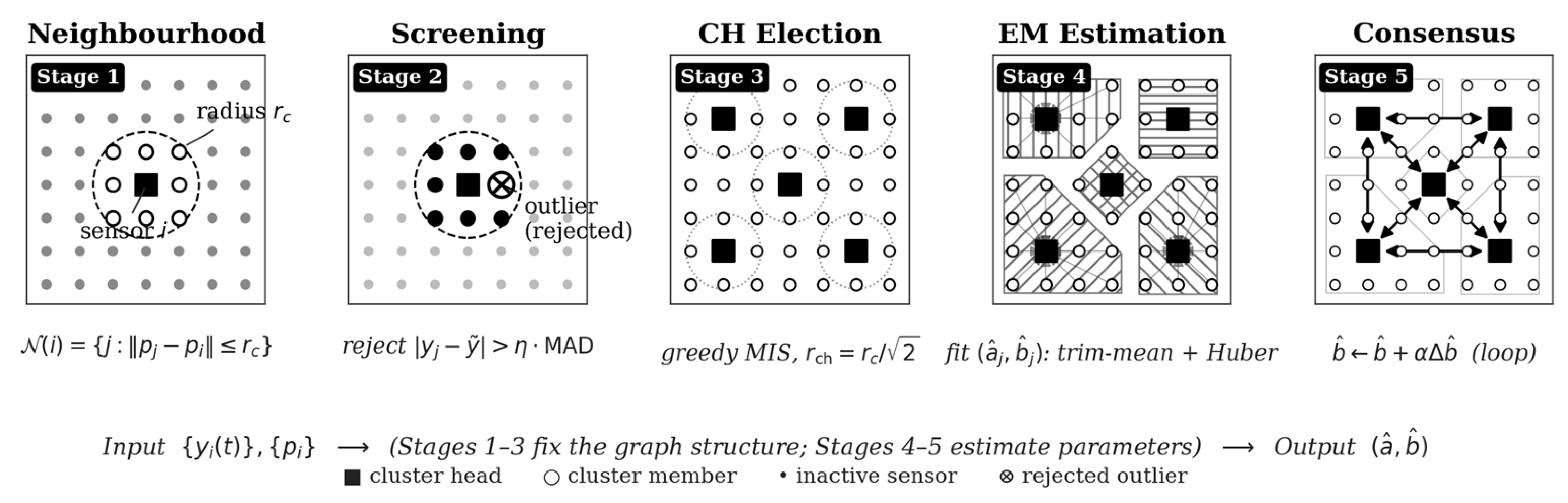
- A principle-based combination of region-based decomposition, robust local estimation and inter-cluster consensus in a five-stage algorithm with deterministic, side-information-free cluster-head election, and explicit convergence properties of all three components are provided.
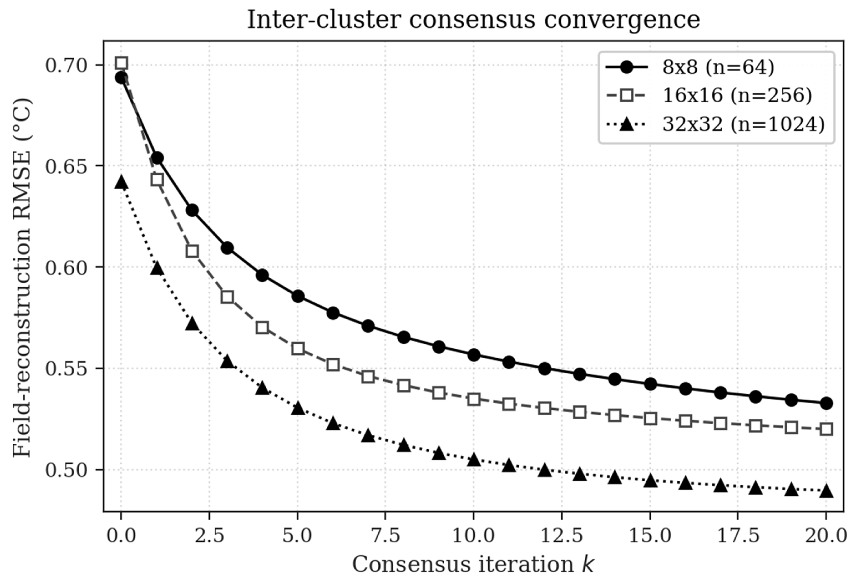
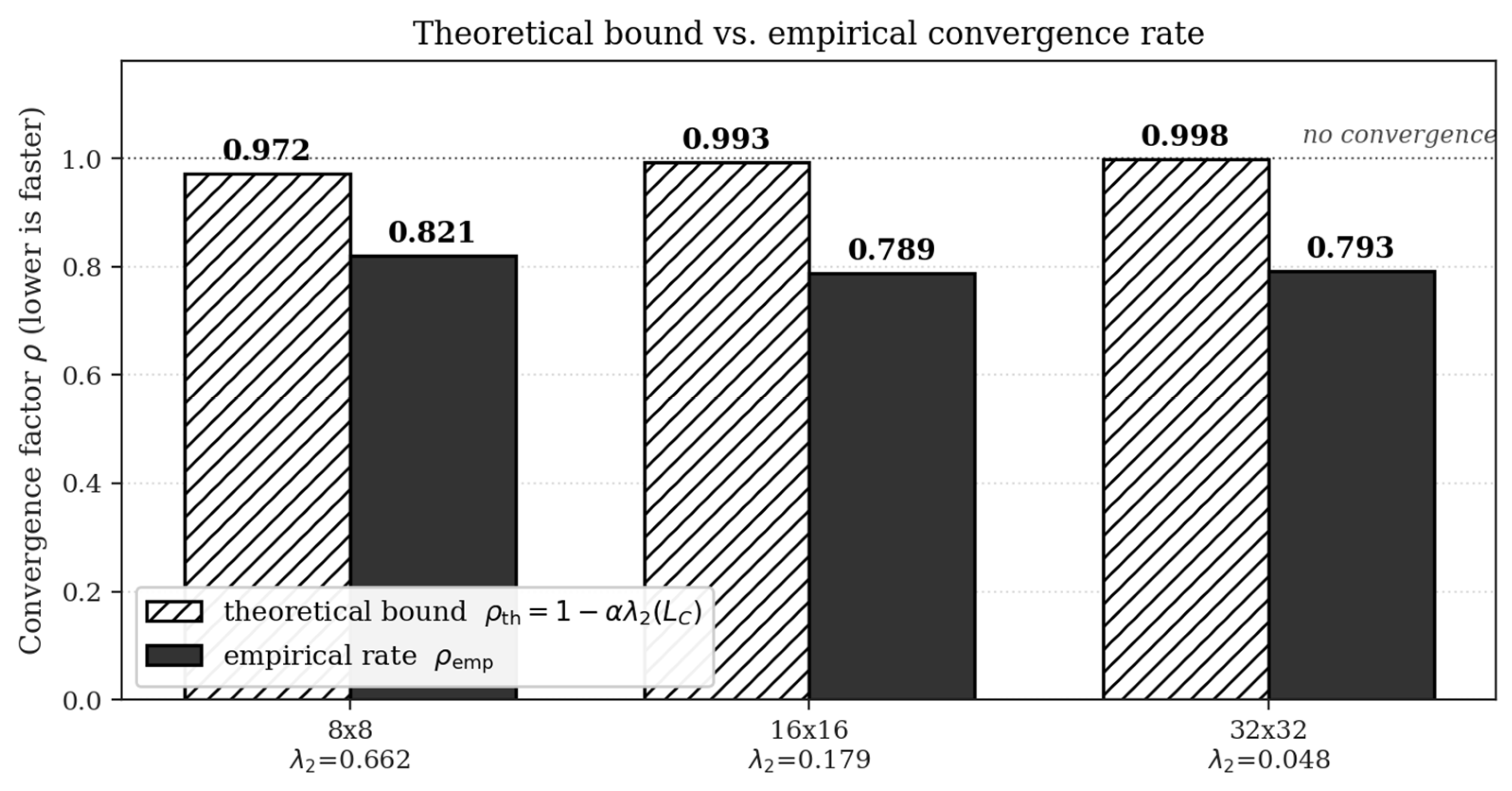
- Three convergence and robustness results adapted to the cluster-overlap setting: (Theorem 1) per-cluster alternating-estimation monotone descent under cluster Hessian positive-definiteness; (Theorem 2) inter-cluster consensus exponential rate ρ ≤ 1 − αλ_2(L_C), specialising the classical Olfati-Saber-Murray result [9] to the cluster-overlap graph; (Theorem 3) finite-sample replacement breakdown of the trimmed-mean field reconstruction.
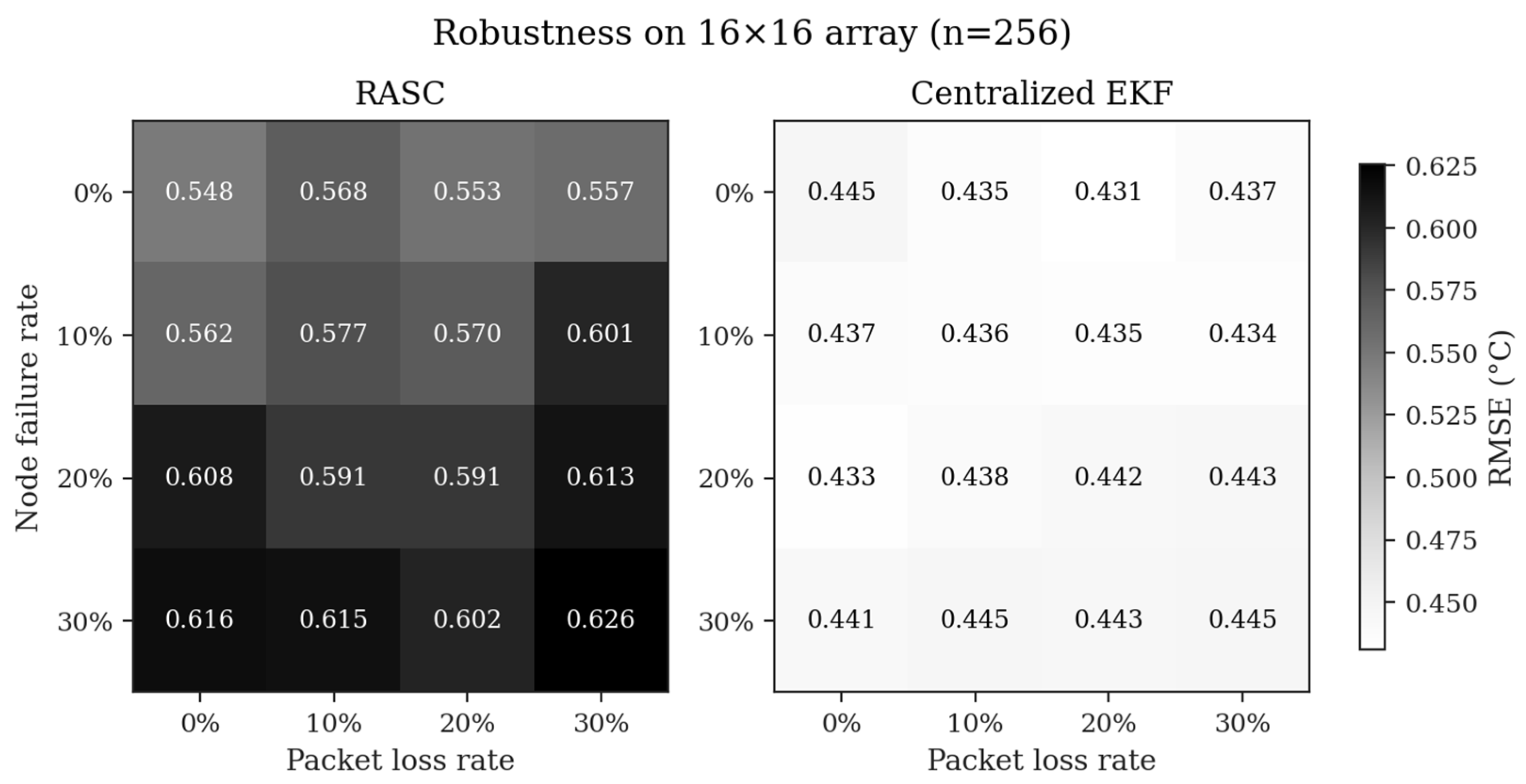
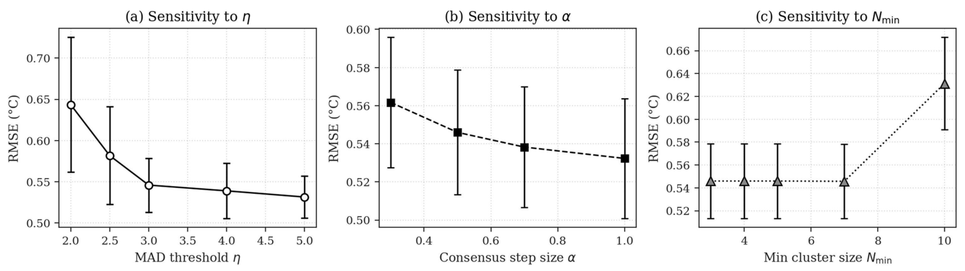
- A total of three array scales were used for comprehensive simulation studies, with 30 independent runs each, and RASC was compared against an oracle centralised extended Kalman filter (EKF) and a faithful re-implementation of the Bychkovskiy–Megerian–Estrin–Potkonjak (BMEP) edge-pairwise calibration baseline [5], as well as four simpler baselines (uncalibrated, temporal smoothing, pairwise differential, and median spatial filter). Robustness and Sensitivity are tested with combined node failure and packet loss, and analysed along η, α and N_min.
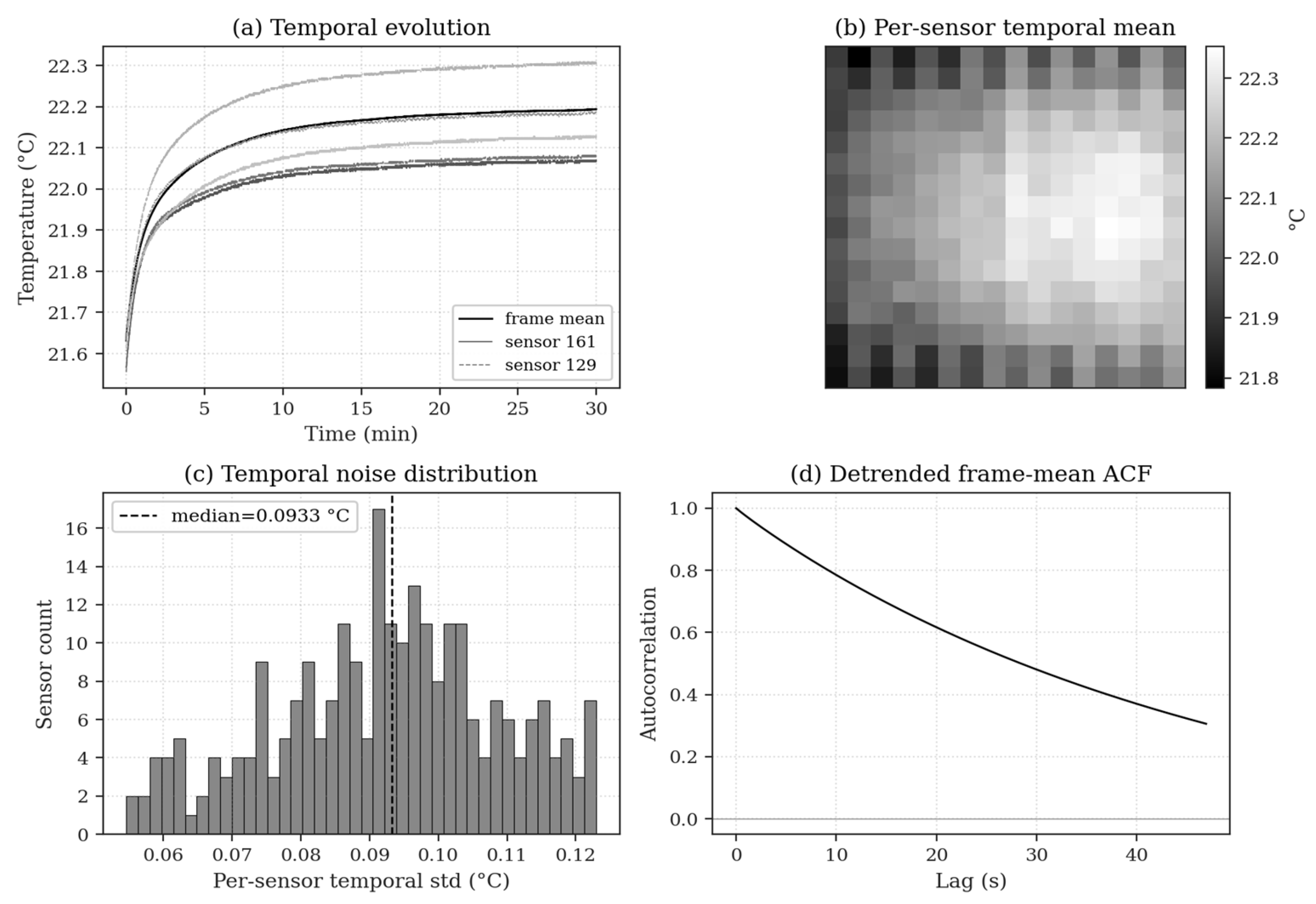
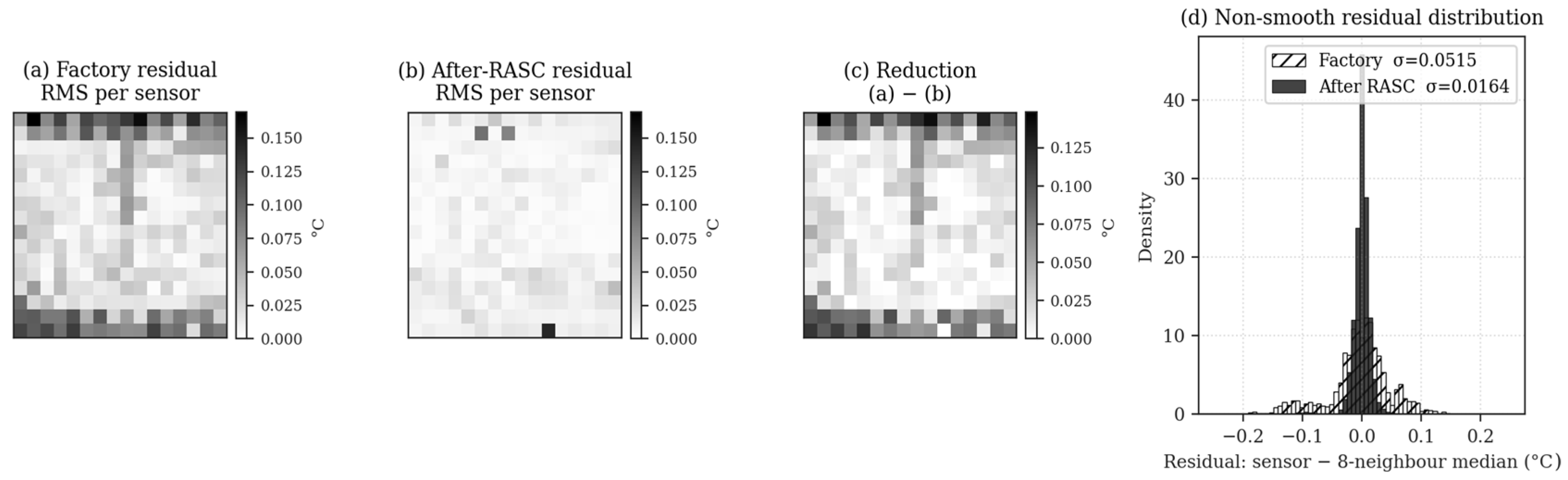
- A real-sensor study of 7632 frames of data from a 16 × 16 BJT-based temperature array on a host PCB showed that the factory ±0.1 °C specification had been exceeded post-deployment (measured a peak-to-peak non-uniformity (NU) of 0.569 °C and about five times the factory specification). RASC is applied to the in situ readings, and the locally non-smooth fixed-pattern residual is reduced by 71 ± 5% (10-fold cross-validation); thus, by this residual metric the array approaches the original factory specification (an inference from local-smoothness residuals, not an independent absolute-accuracy measurement), and only a 0.041 °C RMSE increase in the calibrated field is observed. The decrease is relatively large at the edges of the array (78% vs. 55% in the middle), and this matches the experimental observation.
- An honest discussion of identifiability: Why per-sensor (a, b) recovery is degenerate along a one-dimensional gauge in narrow-range fields even when the reconstructed field is good, and the mitigation offered by reference anchoring, as well as a discussion of when the gauge ambiguity is practically significant.
1.2. Paper Organisation
2. Related Work
2.1. Centralised Non-Uniformity Correction
2.2. Distributed Calibration in WSNs
2.3. Robust and Median-Based Estimation
2.4. Consensus Algorithms
2.5. Learning-Based Calibration
3. Problem Formulation
3.1. Sensor Model
- (A1) Local field smoothness: There is a length scale ℓ such that, in any disc of radius r ≤ ℓ, the field x(·, t) is well-approximated by a single common signal (t).
- (A2) Bounded heterogeneity: a_i ∈ [a_min, a_max] with 0 < a_min, and |b_i| ≤ B for a finite B; both are constant over the calibration time horizon T.
- (A3) Reference anchoring: A subset R ⊂ {1,…,n} of size |R| = ρn, where ρ≪1 (e.g., 5%), consists of known (a_i, b_i) for i ∈ R.
3.2. Identifiability
3.3. Communication Model
4. The RASC Algorithm
4.1. Stage 1: Neighbourhood Formation
4.2. Stage 2: Consistency Screening
4.3. Stage 3: Cluster-Head Election
4.4. Stage 4: Intra-Cluster Alternating Estimation
4.5. Stage 5: Inter-Cluster Consensus
4.6. Pseudocode
| Algorithm 1 RASC: Region-Aware Self-Calibration |
|
Input Y ∈ ℝT×n, coords {p_i}, radius r_c, threshold η, step α, min cluster size N_min, reference set R with values (a_R, b_R) Output estimates (â, ) ∈ ℝn × ℝn 1: build (i) for all i ▷ Stage 1 2: (i) ← consistency-screen(y(), (i), η) ▷ Stage 2 3: CH ← greedy-MIS(score = ||, r_ch = r_c/√2) ▷ Stage 3 4: for each ch ∈ CH do ▷ Stage 4 5: M ← (ch); if |M| < N_min: continue 6: initialize â_M ← 1, _M ← 0 7: for em ← 1..n_em do 8: (t) ← trim-mean_γ { (y_j(t) − _j)/â_j : j ∈ M } 9: for j ∈ M, j ∉ R do 10: (â_j, _j) ← huber-IRLS(y_j, , c = 1.345) 11: end for 12: end for 13: broadcast (â_j, _j) for j ∈ M 14: end for 15: average overlapping estimates per sensor 16: for k ← 1..K_max do ▷ Stage 5 17: compute Δ from (7) over all clusters 18: ← + α · Δ; clamp _R = b_R; clamp â_R = a_R 19: if ‖Δ‖_∞ < tol: break 20: end for 21: return (â, ) |
4.7. Communication Cost
5. Theoretical Analysis
5.1. Per-Cluster Alternating-Estimation Convergence
5.2. Inter-Cluster Consensus Rate
5.3. Robustness with Trimmed Mean
5.4. Communication–Computation Trade-Off
6. Simulation Studies
6.1. Experimental Setup
- Uncalibrated—Raw measurement y_i used as the field estimate.
- Factory—knows true (a_i, b_i) for all sensors, providing the σ-floor lower bound.
- Centralised EKF: A per-sensor 2-state extended Kalman filter that uses oracle access to the true field x(p_i, t) for tracking. This is an idealised centralised baseline assuming loss-free transmission to a fusion centre.
- RASC—our method, with default hyperparameters r_c = 0.10, η = 3, α = 0.5, N_min = 4, γ = 0.20.
6.2. Main Results
6.3. Convergence and Theory Verification
6.4. Robustness
6.5. Comparison with Simple Baselines and BMEP
6.6. Sensitivity Analysis
7. Online Recalibration of a Deployed Temperature-Sensor Array
7.1. Hardware and Acquisition
7.2. Direct Evidence of Post-Deployment Drift
7.3. Online Recalibration Results
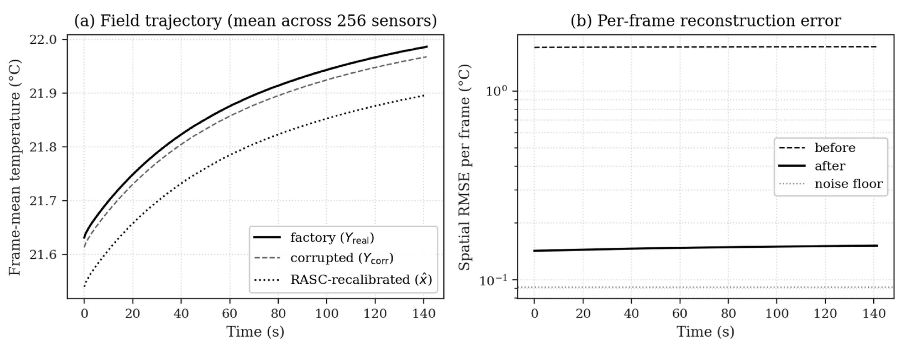
- Field-space stability: RMSE of the post-calibration field = (Y − )/â and the original Y. A good algorithm should change Y by no more than a noise-floor-scale amount.
- Local non-smooth residual: For each sensor and each frame, the deviation of that sensor’s reading from the median of its eight nearest neighbours. This is a model-free proxy for fixed-pattern noise that cannot be explained by a locally smooth physical field; that is to say, precisely what post-deployment drift in (a_i, b_i) produces.
- Edge-vs-interior reduction: The same residual is stratified by location to test the prediction (Section 7.2), and it is found that drift occurs at the edge of the array.
7.4. Semi-Synthetic Stress Test
8. Discussion
8.1. When Does RASC Win, and Against What?
8.2. Identifiability and Gauge Degeneracy
8.3. Connection to Traditional Distributed Calibration
8.4. Limitations
- The local-smoothness assumption (A1) does not hold near sharp thermal edges (e.g., a hot object that only covers part of the array). In such cases, clusters at the boundary will produce biassed _c; although consistency screening eliminates the most severe outliers, it does not address this issue directly. Adaptive clustering that considers the detected discontinuities is a reasonable extension.
- The reference subset R needs to be unchanged in the calibration window. If the reference sensors have drifted, RASC will also have a bias. Periodic refreshing of the reference set against a traceable temperature reference at maintenance intervals—or, in the case of BJT-based arrays, locating reference sensors in mechanically isolated areas of the host PCB to reduce V_BE stress—is recommended for long-term operation. Because RASC anchors the global gauge to the reference subset, the placement and reliability of these sensors directly govern performance, and two practical guidelines follow from the physics of the observed drift. First, since drift is strongest at the array edges (Section 7.3), reference sensors should preferentially be located in the mechanically and thermally quieter interior, away from copper pours, mounting posts and high-dissipation components, so that the anchors are themselves among the least-drifted nodes. Second, because the consensus stage propagates calibration outward from anchored clusters, the reference set should be spatially distributed rather than clustered, so that every region—including the edges—lies within a short consensus reach of an anchor; modest redundancy beyond the minimal anchor count further allows the robust consensus stage to down-weight an individual reference that has itself drifted. Quantitatively, under the edge-concentrated drift observed in this deployment, interior anchor sites carry on average about 1.7× less drift than edge sites, so the factory-value assumption (a, b) = (1, 0) on which the anchors rely is substantially more accurate for interior placement. A reference-set sensitivity study varying the number and placement of anchors confirms this: increasing the reference fraction helps only modestly, and under the observed edge-concentrated drift interior placement attains a lower calibrated-field error (about 0.41 °C) than edge placement (about 0.46 °C); a fuller study sweeping induced-drift models is left for future work.
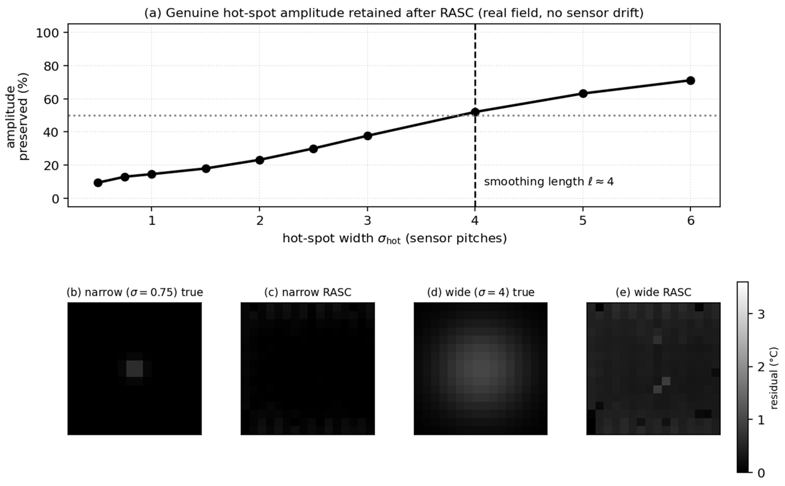
- Assumption (A1) treats the field as locally smooth. In scenes with genuine sub-array-scale structure—localised hot spots or sharp gradients narrower than the smoothing length ℓ—such structure is, at the array’s spatial sampling resolution, not readily distinguishable from per-sensor drift, and RASC may partially absorb it into the calibration; multi-pixel smooth features, by contrast, remain well separated from drift. A dedicated stress test that injects synthetic hot spots and sharp gradients (sweeping feature width against the smoothing length) confirms this behaviour (Figure 13): genuine structure broader than the cluster/smoothing scale is largely preserved (about 71% of the hot-spot amplitude is retained at a Gaussian width of ~6 sensor pitches), whereas sub-ℓ hot spots are progressively absorbed into the per-sensor calibration (about 38% retained near ~3 pitches and about 9% for point-like features near a single pitch), which delimits the validity regime of Assumption (A1) and motivates the edge-aware clustering noted below as future work.
- Based on the linear V_BE temperature dependence of the BJT sensing element, we restricted the analysis to affine drift y = a x + b. Higher-order drift (e.g., gain non-linearity due to severe junction degradation, temperature-dependent offset caused by package thermal-coefficient mismatch) would require extra structure in Stage 4. The Estimation framework can be conveniently extended to a Local Polynomial Model, and the breakdown-point analysis will also need modification.
- Extend the longitudinal validation period of the maintenance and add more data. The recorded analysis here is a single snapshot of post-deployment drift on one host PCB; a follow-up study would be to track the same array over several months and confirm whether RASC is still compensating for accumulated drift, as well as to characterise the rate at which the drift level increases in this hardware family and compare it with the conservative-drift assumptions made in Section 7.4.
9. Conclusions
Author Contributions
Funding
Institutional Review Board Statement
Informed Consent Statement
Data Availability Statement
Conflicts of Interest
Appendix A
Appendix B
Appendix C. Reproducibility
- Source code: rasc_core.py is about 250 lines of NumPy implementing the algorithm, and run_simulation.py is used to reproduce all simulation tables and figures.
- Actual temperature data: 7632 frames, 16 × 16 calibrated temperature-sensor recordings, sampled at 4.241 Hz over 29.99 min. Provided as an .xlsx file containing timestamps.
- Random seeds: Every Monte Carlo cell uses np.random.default_rng(seed) with seed = run_index ∈ {0, …, 29}, so all results are bit-exactly reproducible.
- Hyperparameter defaults: r_c = 0.10, η = 3.0, α = 0.5, N_min = 4, γ = 0.20, n_em = 5, n_irls = 4, c_huber = 1.345, K_max = 10, tol = 0.01 °C, reference fraction ρ = 0.05.
References
- Wei, R.; Lin, H.; Chen, Q.; Huang, G.; Hu, W. A CMOS temperature sensor with a smart calibrated inaccuracy of ±0.11 °C (3σ). Sensors 2023, 23, 5132. [Google Scholar] [CrossRef] [PubMed]
- Qin, C.; Huang, Z.; Liu, Y.; Li, J.; Lin, L.; Tan, N.; Yu, X. An energy-efficient BJT-based temperature sensor with ±0.8 °C (3σ) inaccuracy from −50 to 150 °C. Sensors 2022, 22, 9381. [Google Scholar] [CrossRef] [PubMed]
- Friedenberg, A.; Goldblatt, I. Nonuniformity two-point linear correction errors in infrared focal plane arrays. Opt. Eng. 1998, 37, 1251–1253. [Google Scholar] [CrossRef]
- Ratliff, B.M.; Hayat, M.M.; Hardie, R.C. An algebraic algorithm for nonuniformity correction in focal-plane arrays. J. Opt. Soc. Am. A 2002, 19, 1737–1747. [Google Scholar] [CrossRef] [PubMed]
- Bychkovskiy, V.; Megerian, S.; Estrin, D.; Potkonjak, M. A collaborative approach to in-place sensor calibration. In Information Processing in Sensor Networks (IPSN 2003); Lecture Notes in Computer Science; Springer: Berlin, Germany, 2003; Volume 2634, pp. 301–316. [Google Scholar] [CrossRef] [PubMed]
- Wang, Y.; Yang, A.; Chen, X.; Wang, P.; Wang, Y.; Yang, H. A deep learning approach for blind drift calibration of sensor networks. IEEE Sens. J. 2017, 17, 4158–4171. [Google Scholar] [CrossRef]
- Faghih Niresi, K.; Zhao, M.; Bissig, H.; Baumann, H.; Fink, O. Spatial-temporal graph attention fuser for calibration in IoT air pollution monitoring systems. In Proceedings of the 2023 IEEE SENSORS, Vienna, Austria, 29 October–1 November 2023; pp. 1–4. [Google Scholar] [CrossRef]
- Maag, B.; Zhou, Z.; Thiele, L. A survey on sensor calibration in air pollution monitoring deployments. IEEE Internet Things J. 2018, 5, 4857–4870. [Google Scholar] [CrossRef]
- Olfati-Saber, R.; Murray, R.M. Consensus problems in networks of agents with switching topology and time-delays. IEEE Trans. Autom. Control 2004, 49, 1520–1533. [Google Scholar] [CrossRef]
- Rogalski, A. History of infrared detectors. Opto-Electron. Rev. 2012, 20, 279–308. [Google Scholar] [CrossRef]
- Narendra, P.M.; Foss, N.A. Shutterless fixed pattern noise correction for infrared imaging arrays. In Technical Issues in Focal Plane Development, Proceedings of the Technical Symposium East; SPIE: Bellingham, WA, USA, 1981; Volume 282, pp. 44–51. [Google Scholar] [CrossRef]
- Perry, D.L.; Dereniak, E.L. Linear theory of nonuniformity correction in infrared staring sensors. Opt. Eng. 1993, 32, 1854–1859. [Google Scholar] [CrossRef]
- Harris, J.G.; Chiang, Y.-M. Nonuniformity correction of infrared image sequences using the constant-statistics constraint. IEEE Trans. Image Process. 1999, 8, 1148–1151. [Google Scholar] [CrossRef] [PubMed]
- Lu, D.; Teng, L.; Ren, J.; Tan, J.; Wang, M.; Wang, L.; Gu, G. Scene-based nonuniformity correction method using principal component analysis for infrared focal plane arrays. Appl. Sci. 2023, 13, 13331. [Google Scholar] [CrossRef]
- Ding, S.; Wang, D.; Zhang, T. A median-ratio scene-based non-uniformity correction method for airborne infrared point target detection system. Sensors 2020, 20, 3273. [Google Scholar] [CrossRef] [PubMed]
- Whitehouse, K.; Culler, D. Calibration as parameter estimation in sensor networks. In Proceedings of the 1st ACM International Workshop on Wireless Sensor Networks and Applications (WSNA’02), Atlanta, GA, USA, 28 September 2002; pp. 59–67. [Google Scholar] [CrossRef]
- Takruri, M.; Challa, S. Drift aware wireless sensor networks. In Proceedings of the 10th International Conference on Information Fusion, Quebec City, QC, Canada, 9–12 July 2007; pp. 1–7. [Google Scholar]
- Ahmad, R. Enhanced drift self-calibration of low-cost sensor networks based on cluster and advanced statistical tools. Measurement 2024, 236, 115158. [Google Scholar] [CrossRef]
- Mahajan, S.; Helbing, D. Dynamic calibration of low-cost PM2.5 sensors using trust-based consensus mechanisms. npj Clim. Atmos. Sci. 2025, 8, 257. [Google Scholar] [CrossRef] [PubMed]
- Huber, P.J.; Ronchetti, E.M. Robust Statistics, 2nd ed.; Wiley: Hoboken, NJ, USA, 2009. [Google Scholar]
- Hampel, F.R.; Ronchetti, E.M.; Rousseeuw, P.J.; Stahel, W.A. Robust Statistics: The Approach Based on Influence Functions; Wiley: New York, NY, USA, 1986. [Google Scholar]
- Chandola, V.; Banerjee, A.; Kumar, V. Anomaly detection: A survey. ACM Comput. Surv. 2009, 41, 15. [Google Scholar] [CrossRef]
- Xiao, L.; Boyd, S. Fast linear iterations for distributed averaging. Syst. Control Lett. 2004, 53, 65–78. [Google Scholar] [CrossRef]
- Sirocchi, C.; Bogliolo, A. Topological network features determine convergence rate of distributed average algorithms. Sci. Rep. 2022, 12, 21831. [Google Scholar] [CrossRef] [PubMed]
- Sun, Y.; Zheng, Y. A method of gas sensor drift compensation based on intrinsic characteristics of response curve. Sci. Rep. 2023, 13, 11971. [Google Scholar] [CrossRef] [PubMed]
- Koziel, S.; Pietrenko-Dabrowska, A.; Wojcikowski, M.; Pankiewicz, B. Efficient calibration of cost-efficient particulate matter sensors using machine learning and time-series alignment. Knowl.-Based Syst. 2024, 295, 111879. [Google Scholar] [CrossRef]
- Shao, T. Distributed consensus Kalman filtering for asynchronous multi-rate sensor networks. Signal Image Video Process. 2024, 18, 6419–6429. [Google Scholar] [CrossRef]
- Dempster, A.P.; Laird, N.M.; Rubin, D.B. Maximum likelihood from incomplete data via the EM algorithm. J. R. Stat. Soc. Ser. B 1977, 39, 1–38. [Google Scholar] [CrossRef]
- Chung, F.R.K. Spectral Graph Theory; CBMS Regional Conference Series in Mathematics; American Mathematical Society: Providence, RI, USA, 1997; Volume 92. [Google Scholar]
- Fiedler, M. Algebraic connectivity of graphs. Czechoslov. Math. J. 1973, 23, 298–305. [Google Scholar] [CrossRef]



| Scale | Uncal. | Factory | EKF (Oracle) | RASC | Bytes EKF | Bytes RASC | Clusters |
|---|---|---|---|---|---|---|---|
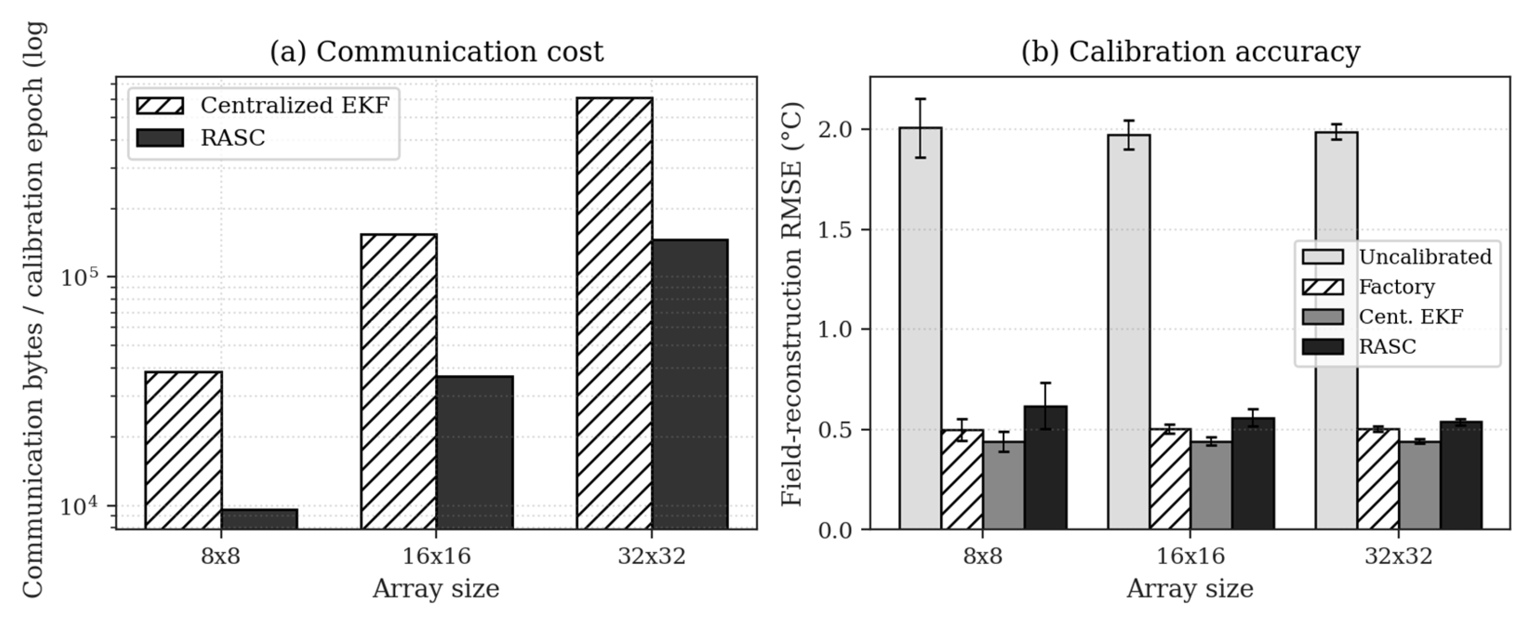
| 8 × 8 | 2.01 ± 0.15 | 0.50 ± 0.05 | 0.44 ± 0.05 | 0.62 ± 0.11 | 38.4 k | 9.6 k | 24.6 |
| 16 × 16 | 1.97 ± 0.12 | 0.50 ± 0.03 | 0.44 ± 0.03 | 0.56 ± 0.05 | 154 k | 36.9 k | 79.0 |
| 32 × 32 | 1.99 ± 0.06 | 0.50 ± 0.02 | 0.44 ± 0.02 | 0.54 ± 0.02 | 614 k | 146 k | 293 |
| Method | Field RMSE (°C) | Comment |
|---|---|---|
| Uncalibrated (raw) | 1.947 ± 0.081 | baseline |
| Temporal smoothing (5-frame moving average) | 1.901 ± 0.080 | spatial structure ignored |
| Pairwise differential (offset only) | 1.538 ± 0.208 | no consensus refinement |
| Median spatial filter (3 × 3) | 0.882 ± 0.071 | no parameter recovery |
| Graph-Laplacian/total-variation (TV) smoothing | 0.87 ± 0.04 | spatial only; structure–accuracy trade-off (Section 6.5) |
| BMEP edge-pairwise [5] | 0.695 ± 0.103 | offset only, gain fixed |
| RASC (this work) | 0.603 ± 0.046 | full (a, b) recovery |
| Factory oracle (true a, b) | 0.502 ± 0.004 | irreducible noise floor |
| Quantity | Factory Y_Real | After RASC | Change |
|---|---|---|---|
| Field RMSE between and Y_real | — | 0.041 ± 0.001 °C | within noise floor |
| Per-frame spatial peak-to-peak | 0.41 °C | 0.30 ± 0.06 °C | −27 ± 14% |
| Local non-smooth residual (RMS) | 0.0517 °C | 0.0149 ± 0.0024 °C | −71.3 ± 4.8% |
| Edge residual (rows 0–1, 14–15) | 0.0923 °C | 0.0205 ± 0.0065 °C | −77.8 ± 7.1% |
| Interior residual (rows 2–13) | 0.0269 °C | 0.0121 ± 0.0008 °C | −54.9 ± 3.0% |
| Quantity | Y_Corr (Corrupted) | After RASC | Reduction |
|---|---|---|---|
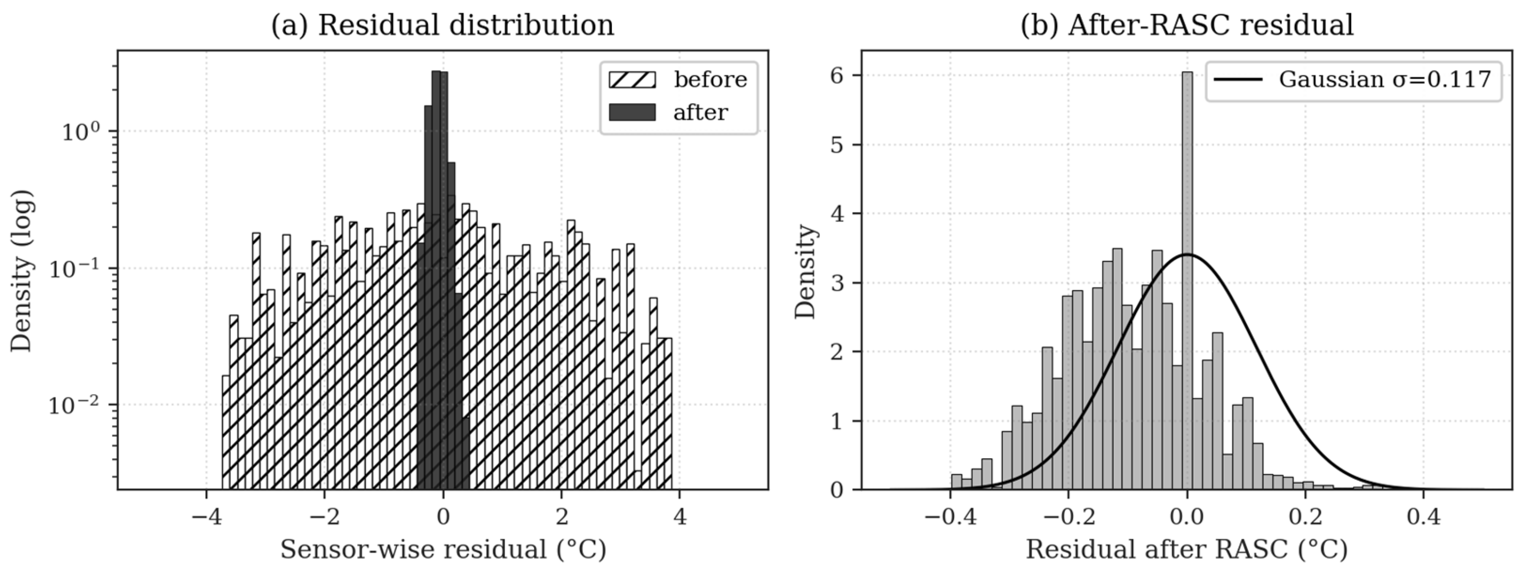
| Field RMSE vs. Y_real | 1.710 °C | 0.148 °C | −91.3% |
| Per-frame spatial peak-to-peak | 7.46 °C | 0.51 °C | −93.2% |
| Distance to noise floor | 18.6× | 1.61× | — |
Disclaimer/Publisher’s Note: The statements, opinions and data contained in all publications are solely those of the individual author(s) and contributor(s) and not of MDPI and/or the editor(s). MDPI and/or the editor(s) disclaim responsibility for any injury to people or property resulting from any ideas, methods, instructions or products referred to in the content. |
© 2026 by the authors. Licensee MDPI, Basel, Switzerland. This article is an open access article distributed under the terms and conditions of the Creative Commons Attribution (CC BY) license.
Share and Cite
Ma, Y.; Xiao, F. RASC: Region-Aware Self-Calibration for Dense 2D Sensor Arrays. Electronics 2026, 15, 2724. https://doi.org/10.3390/electronics15122724
Ma Y, Xiao F. RASC: Region-Aware Self-Calibration for Dense 2D Sensor Arrays. Electronics. 2026; 15(12):2724. https://doi.org/10.3390/electronics15122724
Chicago/Turabian StyleMa, Yinglei, and Fei Xiao. 2026. "RASC: Region-Aware Self-Calibration for Dense 2D Sensor Arrays" Electronics 15, no. 12: 2724. https://doi.org/10.3390/electronics15122724
APA StyleMa, Y., & Xiao, F. (2026). RASC: Region-Aware Self-Calibration for Dense 2D Sensor Arrays. Electronics, 15(12), 2724. https://doi.org/10.3390/electronics15122724