Robust and Interpretable Anomaly Detection in Automotive Test Recordings Using Denoising Autoencoders with Adaptive Thresholding

Abstract

The growing complexity of software-defined automotive systems generates massive heterogeneous sensor and ECU data during real and virtual validation, and conventional rule-based analysis of such multivariate time series struggles under dynamic operating conditions, noise, and diverse fault scenarios. Deep learning-based anomaly detection has shown promising performance, yet existing approaches remain limited by static thresholds, insufficient robustness, and reduced interpretability. This study proposes an adaptive framework for intelligent fault detection in test recordings of automotive software systems (ASSs), integrating deep denoising autoencoders (DAEs), adaptive Gaussian thresholding, and explainable artificial intelligence (XAI) techniques. Four DAE architectures (ANN-, RNN-, GRU-, and LSTM-DAE) are systematically evaluated under different noise levels, system versions, and fault conditions, with detection thresholds that adapt dynamically to the statistical behavior of the reconstructed signals, thereby reducing false alarms under varying operating conditions. The framework was evaluated using real-world test recordings from IAV and Hardware-in-the-Loop (HIL)-based digital test drives, where ANN-DAE achieved the most robust detection performance, with F1-scores of 93.91% and 96.39% on the real and virtual test-drive data, respectively. Furthermore, the integration of XAI improved the transparency of anomaly interpretation at the signal level. Overall, the proposed framework shows strong potential for intelligent anomaly detection and quality assurance in safety-critical automotive systems.

1. Introduction

Currently, the automotive industry is undergoing a profound transformation toward software-defined and highly automated vehicles, driven by advances in electrification, connectivity, and intelligent driving technologies [1]. Modern automotive software systems (ASSs) have evolved from predominantly mechanical systems into complex cyber-physical systems, which are characterized by tightly integrated software, electronic control units (ECUs), sensors, actuators, and communication networks [2,3]. This evolution is reflected in the exponential growth of system architecture complexity, which has increased from relatively small codebases in early systems to millions of lines of code in modern vehicles [4]. As a result, ensuring the safety, reliability, and robustness of such complex systems has become a critical challenge [5,6].

In this context, system validation processes in realistic environments play a fundamental role in detecting unseen faults and maintaining adherence to safety standards and operational requirements, i.e., the ISO 26262 standard [7]. However, as a result of conducting such testing approaches under various operational conditions, a massive volume and variety of data are generated [8]. In particular, prototype vehicles and HIL test benches continuously record hundreds of sensor and internal ECU signals during real and virtual driving scenarios [9,10,11]. While such data provide rich information about system behavior, the manual analysis of multivariate numerical time-series data has become impractical due to the volume, noise, and complex temporal dependencies between the signals [12,13].

Conventional approaches to analyzing such test records, including rule-based and threshold-based methods, rely heavily on expert knowledge and manual intervention [14,15]. These methods cannot adapt to various operating conditions, struggle with high-dimensional signal interactions, and are unable to detect emerging and concurrent fault patterns [16]. In industrial practice, for example, during measurement-analysis processes, anomaly detection is typically performed using predefined thresholds, with deviations from expected ranges flagged and corrected using simple heuristics. Although these approaches are effective for identifying extreme deviations, they are inherently inflexible, do not transfer well to different signals or environments, and can lead to information loss due to manual filtering. This motivates the development of an automated approach for detecting anomalies in time-series data from vehicle sensors under various operational conditions in an efficient manner [17,18].

Given the volume and complexity of modern vehicle data, data-driven approaches for fault detection and diagnosis (FDD) based on machine learning (ML) and deep learning (DL) are becoming increasingly important [19]. These methods enable the extraction of knowledge from data patterns and support tasks such as fault detection, anomaly identification, and modeling of system behavior [20]. As a category of data-driven ML methods, unsupervised learning offers the ability to learn system behavior directly from the data and cluster samples based on similarity, reducing the reliance on manual labeling [21]. This challenge is particularly evident in the context of real-world automotive datasets, where the provision and labeling of all possible fault states are impractical.

Recently, data-driven anomaly detection based on autoencoders has emerged as a promising approach for industrial and automotive applications. This is mainly due to its ability to learn a compact representation of normal system behavior and detect deviations based on reconstruction errors [22,23]. Denoising autoencoders (DAEs) further enhance model reliability by training the model to reconstruct clean signals from noisy inputs, which makes them suitable for realistic operating conditions [24,25]. From an automotive engineering perspective, however, the existing literature exhibits three major limitations. First, within the automotive domain, comparing multiple DAE variants under the same experimental conditions during the system validation of ASSs has not been systematically explored. Second, decision thresholds for anomaly values are typically defined as constant, globally tuned values, which can lead to high false-alarm rates or missed detections when operating conditions, system versions, or noise levels change. Third, current autoencoder-based methods are black-box approaches and do not offer insights into the reasons for decision-making or the detection of a specific anomaly. Furthermore, the lack of transparency regarding the analysis process hinders technical acceptance in safety-critical domains.

In parallel, explainable artificial intelligence (XAI) techniques have been proposed to increase the transparency of complex models by mapping predictions to specific input features or time steps [26]. While XAI has already been investigated for supervised classification or simple unsupervised tasks, its integration into DAE-based anomaly detection for high-dimensional sensor data from the automotive industry remains limited [27,28]. At the same time, adaptive thresholding strategies, which dynamically adjust thresholds, have proven effective in reducing false alarms in sensor fault detection and process monitoring. However, such strategies have rarely been integrated into deep learning-based anomaly-detection pipelines to date [29].

In this study, we address the aforementioned gaps by proposing a hybrid adaptive denoising autoencoder framework with XAI for detecting anomalies in complex automotive test-drive data. The proposed framework is evaluated using two complementary use cases: (i) real-world test drives with an instrumented prototype vehicle from the IAV industry and (ii) digital test drives from an HIL environment using real ECUs and high-fidelity system models. The consideration of both real and digital environments enables a comprehensive assessment of model robustness, transferability, and applicability across testing phases. The study systematically investigates anomaly-detection performance under various system versions, noise levels, DAE architectures, and numbers of sensors. Furthermore, it shows the effect of thresholding strategies and XAI integration on detection performance and interpretability. By training the model exclusively with fault-free data, deviations in the reconstruction can be used to identify anomalies and potential faults in unknown datasets. This approach enables the detection of both individual and simultaneous faults in sensor signals obtained from real and simulated test environments.

The main contributions of the proposed framework can be summarized as follows:

• Development of an adaptive DAE-based framework for anomaly detection in the automotive industry, which is applicable to both real prototype and HIL test-drive data and supports multiple network architectures (LSTM-DAE, GRU-DAE, RNN-DAE and ANN-DAE).
• Integration of a dynamic thresholding mechanism based on Adaptive Gaussian Thresholding to ensure stable false-alarm behavior under varying operating conditions, system versions, and noise levels.
• Integration of XAI techniques to provide sensor- and time-localized explanations of anomaly detections, thereby enabling engineers to determine which signals and time intervals contribute most significantly to each detection event.
• Two different case studies were considered, covering both real-world and virtual test drive processes for electric vehicles (EVs) and internal combustion engine (ICE) vehicles, respectively.
• Comprehensive analysis of the effects of changes in system versions, noise levels, DAE architectures, and the number of input sensors on the detection performance and interpretability of the proposed DAE in both real-world and HIL use cases.

The remainder of the article is structured as follows: Section 2 provides a comprehensive overview of the state of the art and highlights the most important contributions as well as the limitations in this field. Section 3 presents the proposed methodology, including details of the model architecture. Section 4 describes the experimental setup as well as the datasets, architectures, thresholding techniques, and XAI methods used. The experimental results are presented and discussed in Section 5, and Section 6 concludes the article and outlines future research directions.

2. Related Work

In this section, the main contributions of related work addressing the problem of anomaly detection in ASSs are presented, highlighting the limitations and gaps associated with existing methods.

Driven by the rapid progress of data-driven ML and DL techniques, numerous intelligent fault-detection approaches have been introduced with lower implementation complexity and high performance compared with traditional model-based methods. Within the automotive domain, several ML techniques, e.g., SVM, ANN, PCA, and RF, have been investigated for various levels of testing in ASSs. For example, focusing on multi-sensor autonomous vehicle systems, the SVM-based method proposed in [30] reported average fault-detection and identification accuracies of 94.94% and 97.01%, respectively. In the same manner, ANN-based diagnostic methods were employed in [31] for internal-combustion-engine fault diagnosis, where injector faults were isolated using statistical and frequency-domain analysis applied to real-world datasets.

With the advancement of DL techniques and their ability to handle massive amounts of data, increasing attention has been directed towards developing intelligent deep-neural-network-based FDD models using historical operational data. Studies that mainly concentrate on post-manufacturing operational scenarios, i.e., real test drives, have reported high achievements using DL methods. For example, the applicability of 1D CNN and multi-class DNN architectures for concurrent fault diagnosis was investigated in [32], where high classification performance was achieved using real-world automotive datasets. Focusing on electric vehicle systems, an LSTM-based FDD framework targeting short-circuit and open-circuit faults in EV systems was introduced in [33] using datasets generated through VIL simulations, where the proposed approach outperformed conventional diagnostic techniques.

On the other hand, during the development and validation phases of automotive systems, a hybrid CNN-LSTM architecture was proposed in [12] for analyzing sensor-related faults during HIL validation activities, i.e., requirement-based testing. The obtained results demonstrated approximately 5% improvement in diagnostic performance compared with standalone DL structures. In the same context, but focusing on another testing method, a CNN-LSTM-based denoising autoencoder (DAE) architecture has been proposed in [25] for intelligent analysis of B2B testing results, achieving an MSE of 0.00312 at 10% noise. Likewise, an intelligent diagnosis framework based on RF and focusing on air-brake systems was proposed in [34]. Using datasets generated from HIL simulations, the proposed method achieved a classification accuracy of 92%. Aiming at handling the problem of concurrent fault detection within the real-time validation process of ASSs, a GRU-based DAE combined with k-means clustering has been proposed in [24]. Compared with conventional clustering approaches, the proposed method demonstrated improved clustering performance. Despite achieving high clustering accuracy, the proposed method remained restricted to signal-level analysis without providing contextual interpretation of the detected anomalies.

In recent years, autoencoder-based anomaly-detection approaches have attracted increasing attention in automotive data analysis, particularly in cases where labeled datasets are not available. In this context, Von Schleinitz et al. [35] proposed the VASP-based fault-detection framework, combining VAE reconstruction with LSTM-based prediction. Focusing on the analysis of motorsport telemetry data, the reported results showed a considerable reduction in prediction error under faulty operating conditions. Nevertheless, the study did not address explainability aspects or concurrent fault scenarios. In the context of connected and automated vehicles, Wang et al. [36] introduced the LAGMM framework for trajectory anomaly detection by integrating density estimation with representation learning of an autoencoder. Furthermore, to enhance temporal feature-extraction capability, a D-CNN-LSTM autoencoder architecture has been proposed in [37]. However, neither study investigated explainability mechanisms nor considered an adaptive threshold within automotive validation environments.

The limited interpretability associated with anomaly-detection approaches has motivated growing interest in integrating XAI techniques with reconstruction-based models. For instance, Rüttgers et al. [38] proposed the ARCANA framework for root-cause analysis of anomalies detected using autoencoders. Besides, interpretability-aware loss functions have been introduced by Jiang et al. [39] to enable feature-level anomaly localization. Other studies incorporated SHAP-based explanation mechanisms into deep autoencoder frameworks, aiming to enable interpretation of the prediction output [40,41]. Although these methods have played a vital role in providing explainability, their applications have remained mainly limited to industrial and communication datasets rather than automotive HIL validation systems.

Based on the reviewed literature, several limitations can still be identified in current intelligent fault-detection approaches during the real-time validation of ASSs. Specifically, many reconstruction-based anomaly-detection methods either lack semantic interpretability of anomalous behavior or depend on constant static thresholds. To address these limitations, the present study proposes an intelligent and explainable framework to be integrated within the real-time validation process of ASSs at the system level, i.e., during real and virtual test drives. The proposed methodology combines adaptive DAE-based anomaly detection with XAI techniques to provide explainable fault interpretation under realistic automotive validation conditions.

3. Methodology

In this section, the proposed framework is presented, including real-time HIL simulation, FI framework, data analysis, and management.

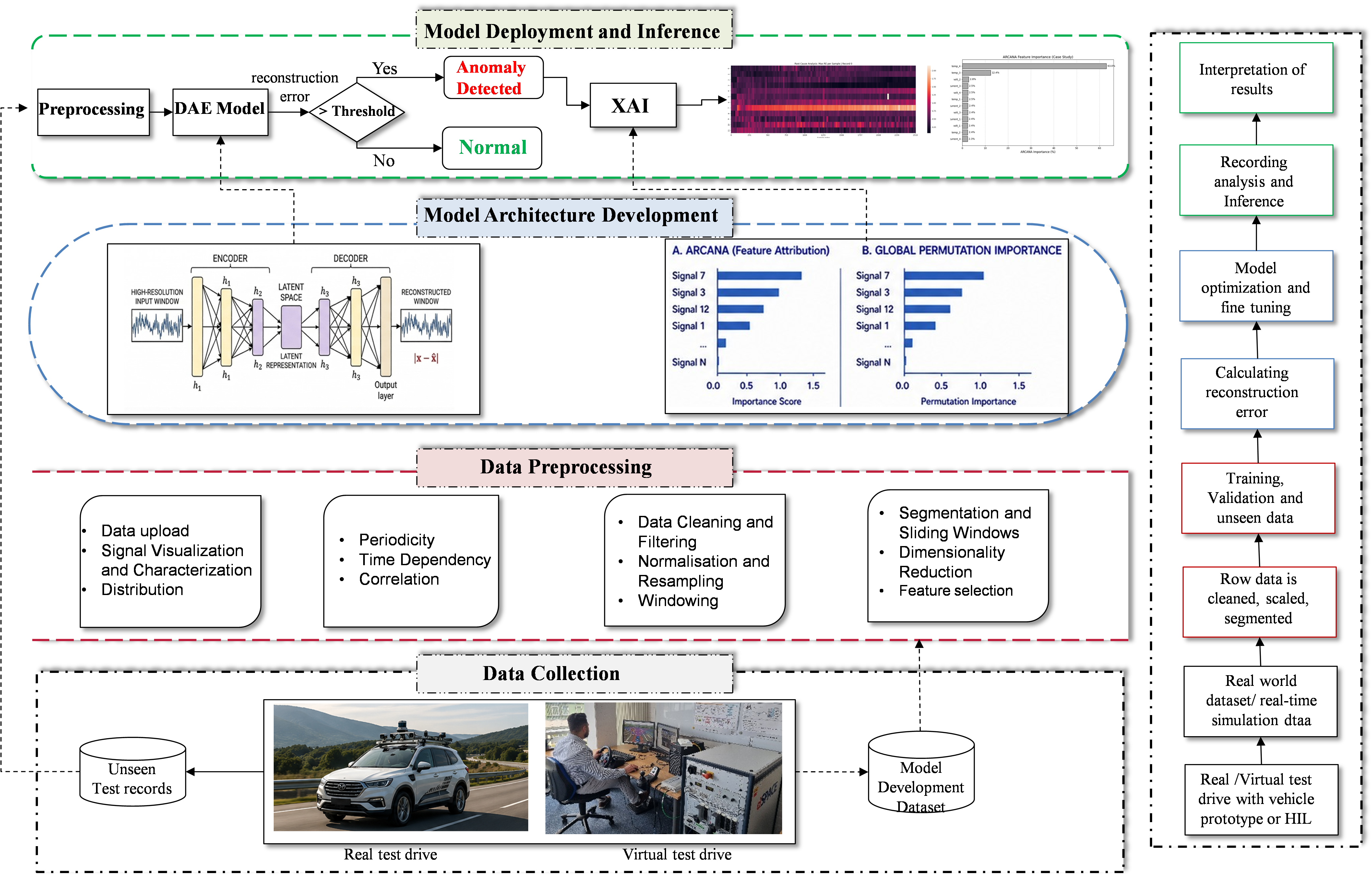
The proposed methodology for developing an intelligent and explainable DAE-based framework for analyzing automotive validation recordings is illustrated in Figure 1. It consists of two main phases: model development and deployment with inference. The development phase consists of four stages, including data collection, data preprocessing, DAE model development, and explainability-analysis development. On the other hand, the deployment phase includes monitoring and analysis activities of unseen test recordings in which the developed framework is employed for anomaly detection and interpretation.

3.1. Data Collection

In the first phase of the proposed framework, the collection of multivariate temporal signals from real-world and virtual driving activities is performed. By conducting real test-driving activities, the system behavior of a real vehicle prototype under realistic traffic and environmental conditions is monitored and captured. On the other hand, the virtual driving environment developed in [42] is employed for conducting digital test drives using a real-time HIL simulation system interacting with ECUs under controlled operational conditions. The generated test recordings from both test-drive activities include measurements of system variables related to vehicle dynamics, sensor outputs, communication variables, control commands, and actuator responses.

To verify the generalization capability of the proposed framework, multiple operational scenarios generated under different driving conditions are included in the dataset. The collected data are divided into model-development records and unseen deployment records. While the model-development dataset is employed for training and validation processes, the unseen records are used for runtime evaluation during the deployment phase.

It should be emphasised that the DAE models are trained independently on the healthy data of the respective setting for each test environment. The real test-drive and HIL recordings differ substantially in their data distributions, including the sampling rate (100 Hz versus 1000 Hz), the selected signal sets, the vehicle type, and the noise characteristics. Direct transfer of trained weights between the two settings is therefore not pursued; instead, the transferability claim refers to the methodology, comprising preprocessing, DAE-based reconstruction, and adaptive thresholding, which is applied unchanged in both environments.

3.2. Data Preprocessing

Once the data-acquisition process is completed, a preprocessing pipeline is applied to improve the quality and consistency of the recorded signals. Due to various real environmental conditions, automotive signal recordings generally contain inconsistent timestamps, redundant variables, corrupted measurements, and noise introduced by sensing and communication layers. Therefore, the preprocessing phase becomes necessary before model development. The higher the quality of the training dataset, the higher the capability of the model to learn representative behavioral patterns [43].

The preprocessing phase starts with a data-cleaning and filtering process, in which incorrect measurements, NaN values, or incomplete values are removed to prevent the model from learning misleading patterns. Furthermore, only the signals relevant to the objectives of this study are considered. Specifically, in the case of real-world test-drive datasets, current, voltage, temperature, and vehicle operational-state signals are considered, whereas irrelevant variables are excluded. By doing so, the computational complexity can be reduced while improving the quality of the developed models.

Following the cleaning phase, all retained signals are normalized using min-max normalization in order to address the large variation in signal magnitudes among current, voltage, and temperature measurements [44].

Mathematically, given a time-series dataset $x=\{x_1,x_2,\dots ,x_T\}$, the normalized signal $\tilde{x}$ is computed as follows:

$${\tilde{x}}_t=2\left({\displaystyle \frac{x_t-\min \left(x\right)}{\max \left(x\right)-\min \left(x\right)}}\right)-1,t=1,\dots ,T$$

(1)

where $\min \left(x\right)$ and $\max \left(x\right)$ are the minimum and maximum of the signal over the recording, and T is the sequence length. This transformation maps all values to the interval $[-1,1]$ while preserving the temporal behaviour of the signal. In addition, the recordings are resampled to ensure consistent sequence lengths across all measurements, since the durations of the recordings vary depending on the driving scenarios. These operations contribute not only to improving numerical stability and model convergence, but also to ensuring structural consistency of the input data.

To further improve robustness against noise, an average smoothing operation based on a sliding window of size w is applied [45]. This process reduces high-frequency fluctuations while preserving the overall temporal trends of the signals. Subsequently, the recordings are segmented into fixed-length temporal windows using a sliding-window strategy. This segmentation transforms long recordings into standardized subsequences suitable for DL-based learning and increases the number of training samples available for model development.

Due to the high dimensionality and redundancy of the recorded signals, a dimensionality-reduction and feature-selection process is performed. In total, four current signals, four voltage signals, and four temperature signals are selected from the available measurements of a real test drive. On the other hand, throttle position, engine temperature, mean effective torque, engine rpm, rail pressure, and vehicle speed variables are selected from the available measurements of a virtual test drive. The selection is based on identifying representative variables among groups of correlated signals while preserving the most informative operational characteristics of the system. This process reduces computational complexity, improves model generalization, and enhances interpretability.

To improve the robustness and generalizability of the developed model under realistic operating conditions, Gaussian noise is introduced into the dataset during the training and evaluation phases. In industrial practice, sensor measurements are often affected by interference and unfavorable acquisition conditions. By incorporating artificial noise, the model can therefore learn representative patterns even in the presence of signal interference and noisy measurements [46]. Gaussian noise is defined as a random variable generated from a Gaussian distribution with mean zero and variance ${\sigma }^2$. By incorporating Gaussian noise of varying intensity, it is possible to assess the extent to which the proposed approach is capable of detecting the fault under noisy operating conditions. Furthermore, evaluating the model using progressively increasing noise levels facilitates the assessment of its stability and robustness when processing incomplete sensor measurements. Such robustness is particularly important for practical applications where measurement uncertainties and environmental disturbances can significantly affect the acquired signals.

Finally, the preprocessed dataset is divided into three portions. Specifically, one part is used for training the target model with 80% of the data, while the second and third parts with 10% each are used for the validation and testing process.

3.3. Model Architecture and Development

The target anomaly-detection model should meet the requirements of providing high detection capability under different driving scenarios while considering noisy operational conditions. Recently, DAE architectures from DL have shown promising performance in overcoming various challenges related to anomaly detection, feature extraction, dimensionality reduction, and noise suppression in industrial monitoring applications [47]. Therefore, the DAE architecture was selected in this study due to its capability to learn representative latent features corresponding to healthy operational behavior.

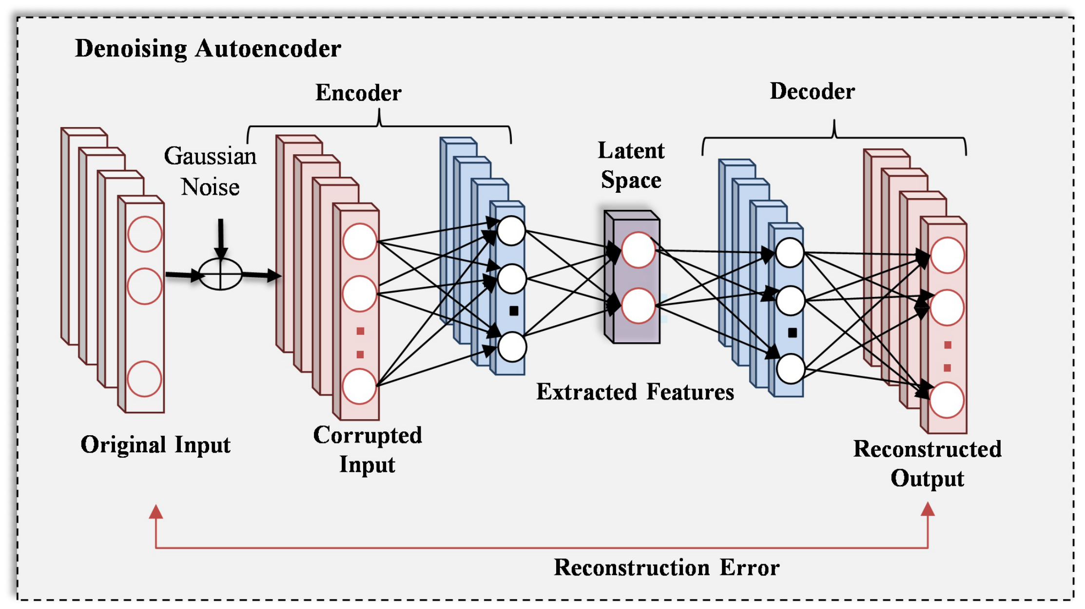
The adopted DAE architecture consists of an input layer, corrupted input layer, encoder layers, latent-representation layer, decoder layers, and reconstructed-output layer, as illustrated in Figure 2. The model was developed to extract representative temporal features and store them in the latent space, reconstruct the original signals, and identify deviations in unseen operational recordings based on the learned healthy patterns.

Once Gaussian noise has been added to the original input sequence, the encoder starts transforming the high-dimensional noisy data into a reduced latent representation in which the representative behavioral characteristics are stored. By using healthy operational data during training, the DAE model learns to denoise and reconstruct the input data efficiently. During optimization, the reconstruction loss between the original signal and the reconstructed output is minimized. The original input sequence is represented as follows:

$$\mathbf{X}=\{{\mathbf{x}}_1,{\mathbf{x}}_2,\dots ,{\mathbf{x}}_T\}$$

(2)

where ${\mathbf{x}}_t$ is the vector of selected signals at time step t, and T is the sequence length.

The corrupted input data are generated according to Equation (3)

$$\tilde{\mathbf{X}}=\mathbf{X}+\mathit{ϵ},\mathit{ϵ}\sim \mathcal{N}(\mathbf{0},{\sigma }^2\mathbf{I})$$

(3)

where $\mathit{ϵ}$ is a noise vector drawn from a Gaussian distribution with zero mean and variance ${\sigma }^2$, and $\mathbf{I}$ is the identity matrix.

The encoder transforms the corrupted sequence into a latent representation according to Equation (4)

$$\mathbf{h}=f({\mathbf{W}}_{\mathrm{e}}\tilde{\mathbf{X}}+{\mathbf{b}}_{\mathrm{e}})$$

(4)

where $\mathbf{h}$ denotes the latent representation, ${\mathbf{W}}_{\mathrm{e}}$ the encoder weight matrix, ${\mathbf{b}}_{\mathrm{e}}$ the encoder bias vector, and $f(·)$ the nonlinear activation function.

On the other hand, the decoder reconstructs the original sequence from the latent representation according to Equation (5)

$$\widehat{\mathbf{X}}=g({\mathbf{W}}_{\mathrm{d}}\mathbf{h}+{\mathbf{b}}_{\mathrm{d}})$$

(5)

where ${\mathbf{W}}_{\mathrm{d}}$ and ${\mathbf{b}}_{\mathrm{d}}$ are the decoder weight matrix and bias vector, $g(·)$ is the activation function, and $\widehat{\mathbf{X}}$ is the reconstructed output sequence.

During the training process, the DAE model is optimized so that the reconstruction loss between the original and reconstructed signals is minimized. The model is optimised by minimising the reconstruction loss,

$$L_{\mathrm{rec}}={\displaystyle \frac{1}{N}}{\displaystyle \sum _{i=1}^N}{∥{\mathbf{X}}_i-{\widehat{\mathbf{X}}}_i∥}^2$$

(6)

where N denotes the number of training samples, and ${\mathbf{X}}_i$ and ${\widehat{\mathbf{X}}}_i$ are the i-th original and reconstructed samples, respectively.

Due to the fact that the DAE model is trained using only healthy data, the network learns the characteristics of normal system behavior. During the deployment phase, any deviation in the calculated reconstruction error of unseen faulty data indicates the presence of an anomaly.

3.4. Model Deployment and Inference

The deployment phase represents the runtime operational stage of the proposed framework. During execution, unseen test recordings are continuously acquired from the monitored system and processed using the same preprocessing pipeline employed during model development. The processed windows are then forwarded to the trained DAE model for reconstruction-based analysis. If the reconstruction error remains below the adaptive threshold, computed from the local statistics of the error signal, the operational condition is identified as normal; otherwise, the corresponding sequence is marked as anomalous and routed to the explainability module.

The deployment workflow supports online inference and continuous monitoring in both real and HIL-based validation environments. The final analysis stage comprises recording interpretation, anomaly visualization, and model refinement, whose feedback into model development closes the diagnostic loop. The generated outputs support validation engineers during fault investigation, model optimization, and test assessment activities. Since the DAE is trained exclusively on healthy data, the framework remains applicable even when fault labels are incomplete or unavailable, while the integrated explainability module links each detection to the contributing signals.

4. Case Study and Experimental Implementation

To verify the applicability of the proposed framework, this section presents selected case studies, highlighting the structure of the datasets and the implementation steps. In this study, two different case studies were examined to cover both real-world and virtual test drive processes of electric vehicles (EVs) and internal combustion engine (ICE) vehicles, respectively. In Case Study 1, sensor signal measurements from a real-world test drive conducted by IAV GmbH on a public road using a real vehicle prototype were analyzed. On the other hand, in Case Study 2, the test data from a virtual environment based on a real-time HIL simulation with a real ECU was considered.

4.1. Case Study 1: Real Test Drive

4.1.1. Test Setup and Measurement Analysis Environment for the Real Test Drive

In the automotive sector, comprehensive validation procedures are required prior to vehicle commercialization to ensure the quality and reliability of developed systems. In this study, the utilized measurement data were obtained from real-world vehicle test drives performed under different driving conditions in Munich during summer trial trips conducted between June and July 2025. During the experiments, measurement signals were recorded from multiple vehicle subsystems, including the battery system, electric drive components, electric power steering, cooling modules, crash, and system management. Consequently, the generated dataset provides a high-dimensional representation of vehicle operational behavior under realistic driving conditions.

The analysis workflow at IAV GmbH is performed using the industrial TRAVIS framework, which represents an integrated environment for automotive data acquisition, processing, and reporting. The framework imports Measurement Data Format (MDF4) recordings together with configuration metadata and processes the data through modular Python v3.10-based scripts for signal extraction and anomaly analysis. The generated outputs are subsequently transformed into structured reports and graphical visualization to support engineering evaluation.

Within the existing workflow, anomaly detection relies predominantly on conventional rule-based thresholding methods. In this approach, a signal sample $x_t$ is classified as anomalous whenever the predefined operational limits are violated: A sample $x_t$ is flagged as anomalous whenever it violates the predefined operational limits,

$$x_t<L_{\min }\mathrm{or}{x}_t>L_{\max }$$

(7)

where $L_{\min }$ and $L_{\max }$ denote the lower and upper operational thresholds derived from engineering safety constraints.

Although static thresholds enable basic filtering of abnormal measurements, their applicability remains limited for dynamic and high-dimensional automotive signals due to the inability to adapt to changing operational conditions. Furthermore, the continuous manual adjustment of numerous signal limits introduces additional maintenance complexity within the engineering workflow.

4.1.2. Dataset Description

The utilized measurements are provided in MDF4 format, which is widely employed in the automotive industry for storing high-frequency sensor and ECU recordings. The analyzed dataset contains 531 measurements with a total size of approximately 29.5 GB, where individual recordings range from nearly 2 MB to more than 450 MB.

Within the scope of this study, the analysis focuses on selected electrical and thermal signals, including current, voltage, and temperature measurements. To improve computational efficiency, large recordings were filtered during loading, and raster-based sampling was applied to reduce memory overhead. The final dataset organization follows the industrial framework, where each column corresponds to a sensor signal, and each row contains the associated time-series observations.

4.1.3. Data Exploration and Statistical Analysis

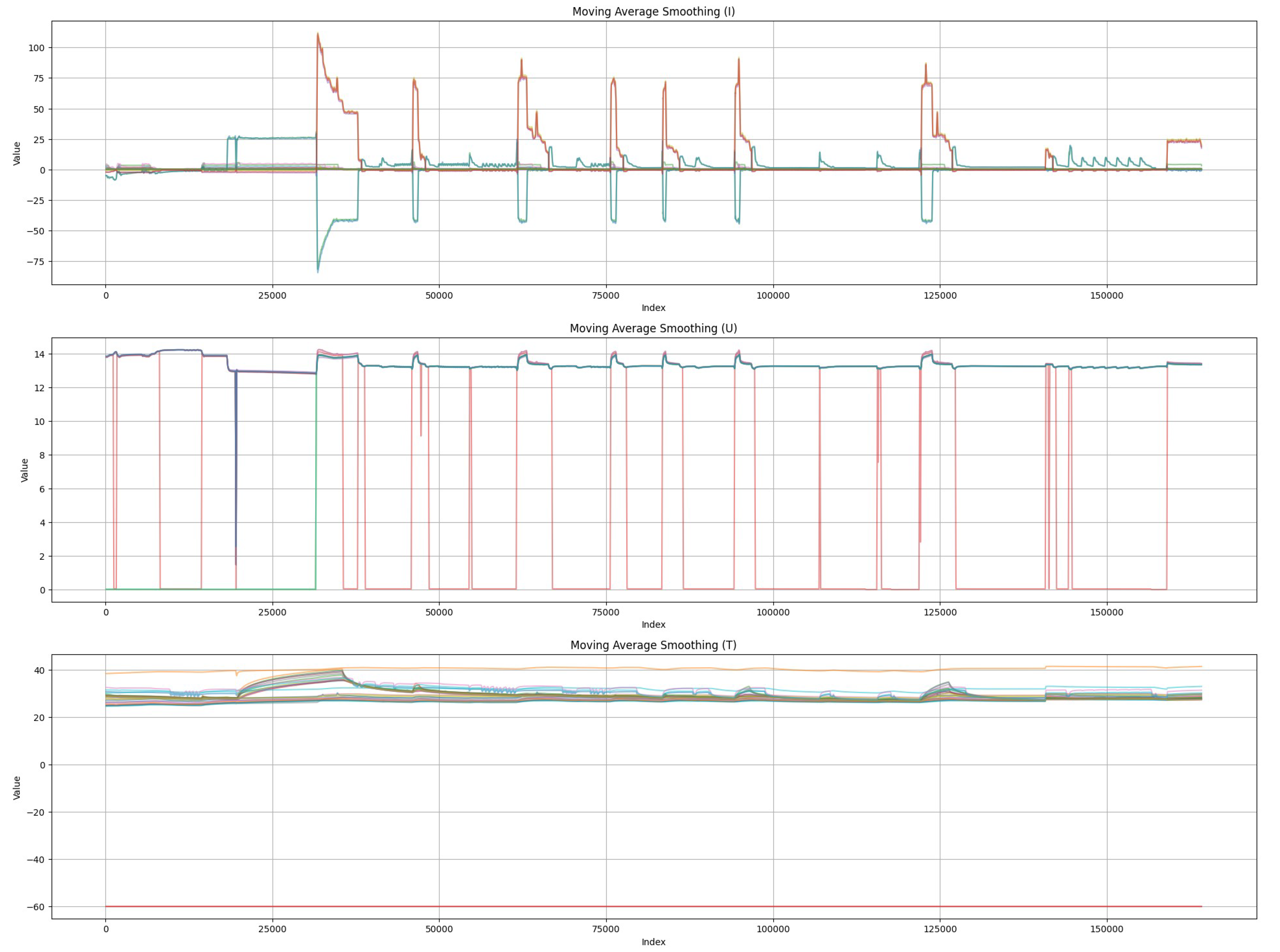
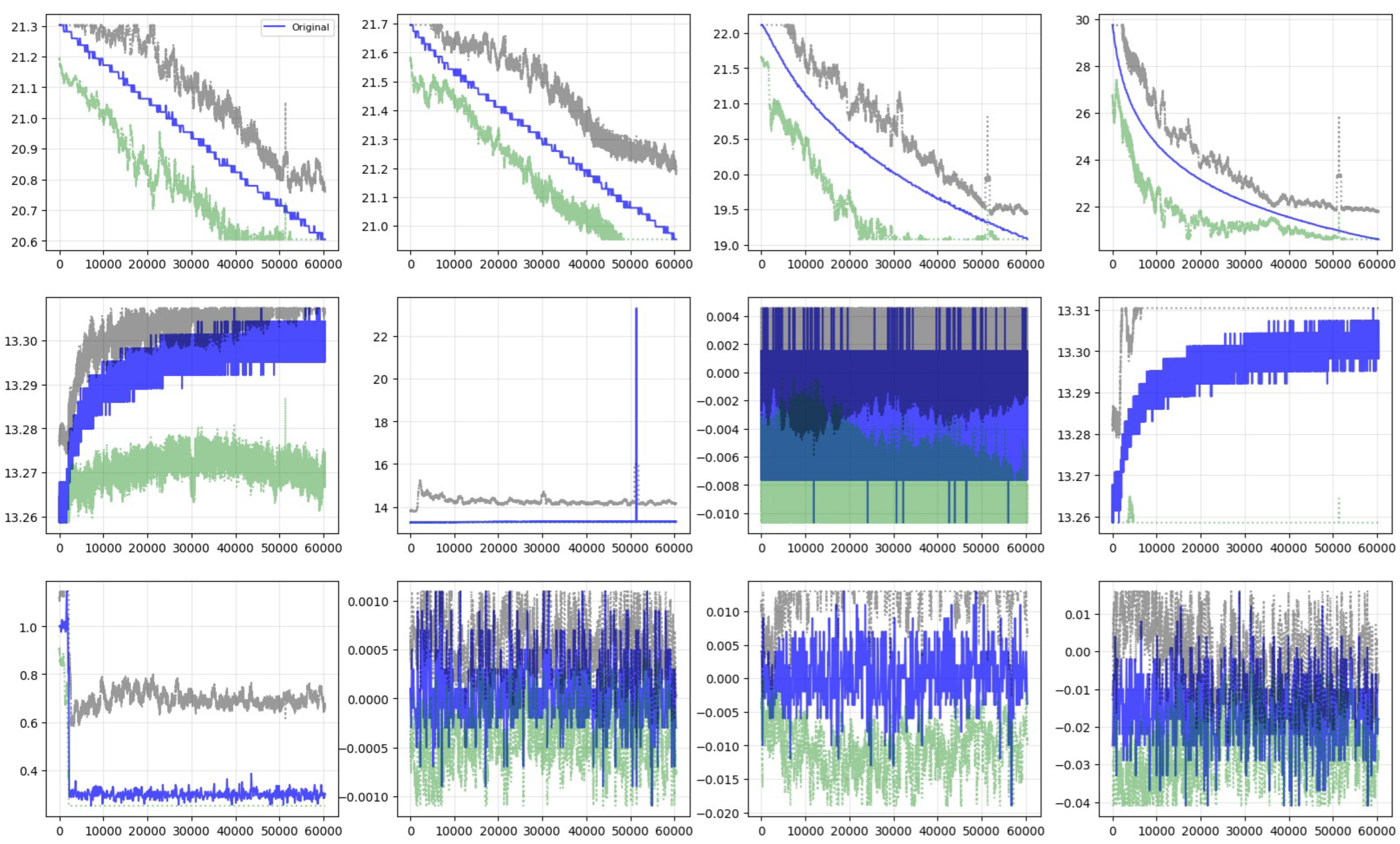
Several exploratory analyses were conducted to investigate the statistical and temporal characteristics of the recorded measurements. The analyzed signals include temperature, current, voltage, subsystem-state, and operational vehicle measurements sampled at 100 Hz. The raw behavior of representative current, voltage, and temperature signals before preprocessing is illustrated in Figure 3, Figure 4 and Figure 5. Temperature measurements generally exhibit smooth long-term variations, whereas current and voltage signals contain abrupt fluctuations and transient peaks during vehicle operation.

Trend analysis is performed using a moving-average smoothing operation,

$${\overline{x}}_t={\displaystyle \frac{1}{w}}{\displaystyle \sum _{i=t-w+1}^t}{x}_i$$

(8)

where ${\overline{x}}_t$ is the smoothed signal and $w=100$ is the selected window size. The results indicate that voltage and temperature signals exhibit relatively smooth long-term behaviour, whereas current signals demonstrate higher variability, as can be seen in Figure 6. It has been observed that most signals do not follow standard statistical distributions due to varying operational conditions, road characteristics, and sensor diversity.

Temporal dependency was evaluated using the autocorrelation function (ACF). Temperature and voltage measurements demonstrated strong temporal correlation, whereas current signals exhibited more diverse dependency behavior. Correlation analysis based on the Pearson correlation matrix identified strong relationships between measurements originating from identical subsystems. Based on these observations, a representative subset of 12 signals was selected for the subsequent modeling stage to reduce computational complexity while preserving operational variability.

The pronounced fluctuations of the current signals reflect instantaneous load changes of the connected consumers: the electric power steering current responds to steering manoeuvres, while the 12 V lithium and intelligent battery currents follow acceleration and recuperation phases. Voltage dips and ripple on the 12 V rails indicate the stability of the low-voltage supply. These quantities are directly linked to relevant fault mechanisms, including increased contact resistance, harness and connector degradation, and supply instabilities, all of which manifest as abnormal current draw or voltage deviations. Transient voltage spikes are therefore safety-relevant indicators for the integrity of the low-voltage system.

The selection follows two engineering principles. First, the twelve signals cover the three dominant physical domains of the monitored subsystems, namely electrical current, electrical potential, and temperature, across functionally distinct components (battery system, power steering, control equipment, and integration modules), so that faults originating in different subsystems produce observable signatures. Second, each retained signal acts as the representative of a group of strongly correlated measurements identified through the Pearson correlation analysis; deviations affecting an excluded signal of a group therefore propagate to its retained representative. The selected subset thus preserves the operational variability of the full measurement set while reducing the input dimensionality, as summarized in

Table 1. Final feature selection based on correlation analysis for case study 1.

Signal	Description	Selection Logic
Temp_137	Integration module (Roof/Rear-view)	Representative of roof-level thermal state
Temp_135	Integration module (Roof/Rear-view)	Representative of roof-level thermal state
Temp_01	Control equipment module (Driver footwell)	Representative of lower-vehicle thermal state
Temp_16	Control equipment module (Driver footwell)	Representative of lower-vehicle thermal state
Volt_PH	12 V voltage	Indicator of central system voltage stability
Volt_Batt	12 V battery voltage	Primary low-voltage system indicator
Volt_Pump	Oil pump voltage	Functional component voltage monitor
Volt_Intell	Intelligent battery voltage	Independent voltage trend monitor
Curr_Lith	12 V lithium battery current	High-variance current source
Curr_Intell	Intelligent battery current	High-variance current source
Curr_Steer	Electric power steering current	High-frequency functional current
Curr_ctrl_equip	control equipment module current	Component-specific operational current

.

4.2. Case Study 2: Virtual Test Drive with Hil Simulation

4.2.1. Test Setup and Measurement Analysis Environment for the Virtual Test Drive

To validate the applicability of the proposed framework, a comprehensive automotive case study based on the ASM gasoline engine model from dSPACE [48] was considered. The selected system represents a highly detailed automotive engine architecture designed to capture the operational behavior of modern internal-combustion engines under realistic driving conditions. The ASM gasoline engine incorporates advanced functionalities, including variable spark timing, enhanced combustion-chamber architecture, advanced fuel injection, and an integrated engine-management system responsible for regulating engine performance dynamically.

The engine model was developed and executed within the MATLAB/Simulink 2021b environment and includes multiple interacting subsystems, such as the SoftECU, powertrain, vehicle-dynamics, and environmental models. Dedicated input and output interfaces were additionally integrated to enable communication with the physical ECU within the HiL environment. The ASM framework provided by dSPACE supports comprehensive automotive simulation activities covering engine behavior, vehicle dynamics, electrical systems, and traffic environments.

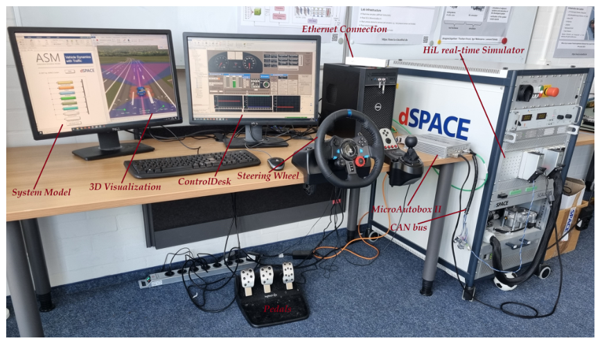
At the hardware level, a HIL platform is used, consisting of dSPACE SCALEXIO and the MicroAutoBox II ECU operating under real-time conditions, as can be seen in Figure 7. The ECU is responsible for generating actuator-control signals associated with fuel injection, rail-pressure management, and injection timing. Communication between the ECU and the SCALEXIO simulator is established through a CAN bus interface. Furthermore, the use case supports both online and offline HIL execution modes through the integration of SoftECU and conventional ECU models. Model implementation, parameterization, execution, and monitoring were additionally supported using ModelDesk v5.6, ConfigurationDesk v6.8, and ControlDesk v7.5.

4.2.2. HIL-Based Data Collection and Dataset Description

Following deployment of the HIL environment, healthy operational behavior was initially recorded during predefined driving scenarios without fault injection (FI). Subsequently, multiple sensor faults were injected into the Accelerator Pedal Position (APP) and engine-speed (RPM) sensors under identical operating conditions. The implemented faults include gain, noise, drift, delay, packet loss, and stuck-at faults. Faults were injected individually and simultaneously during transient intervals between 170 and 330 s, mainly during acceleration and deceleration phases.

The recorded measurement data were initially stored in the proprietary .idv format utilized by ControlDesk and later exported into .csv files for preprocessing and analysis. Each dataset was labeled according to the corresponding fault type and fault location for the model performance verification process. Several variables were monitored throughout the experiments, including throttle position, engine temperature, engine torque, engine speed, manifold pressure, rail pressure, and vehicle velocity. All measurements were sampled at 0.001 s, corresponding to 1000 samples per second. The system variables that have been considered in this study are illustrated in

Table 2. Final feature selection based on correlation analysis for case study 2.

Sensor Name	Unit of Measure	Description
Throttle Position	%	The position of the throttle valve, which indicates the width of the throttle valve opening.
Engine Speed	rpm	The rotational speed of the engine in revolutions per minute.
Intake Manifold Pressure	Pa	Measures the pressure in the intake manifold, indicating the pressure of the air entering the combustion chamber.
Mean Effective Engine Torque	Nm	The average torque of the engine during the entire cycle of combustion.
Rail Pressure	bar	Measures the fuel pressure in the fuel rail.
Engine Outlet Temperature	°C	The temperature of the coolant indicates the effectiveness of the engine’s cooling system.
Vehicle Speed	km/h	The speed of the vehicle in kilometers per hour.

.

4.3. Hyperparameter Optimization

Following data acquisition, preprocessing, and denoising, autoencoder development was conducted. Healthy operational data combined with Gaussian noise were utilized during training, whereas the fault datasets were employed for testing.

Several preprocessing operations were performed before model development, including metadata removal, sensor-label standardization, and standard-score normalization. Subsequently, the datasets were divided into training and testing subsets using an 80:20 ratio. To evaluate robustness under noisy operational conditions, Gaussian noise levels of 1%, 3%, 5%, and 8% were added to the healthy dataset, generating multiple noisy training datasets.

Four deep-learning architectures were investigated for denoising autoencoder implementation, namely GRU-based DAE, LSTM-based DAE, RNN-based DAE, and ANN-based DAE. Each architecture was trained independently using datasets generated under different noise levels.

To optimize the reconstruction performance, hyperparameter tuning was performed using the Ray Tune framework integrated with PyTorch v2.1. The optimized hyperparameters include batch size, learning rate, number of epochs, hidden-layer dimensions, and number of layers. As can be seen in

Table 3. Hyperparameter selection for DAE Models.

Parameter	Range	ANN-DAE	LSTM-DAE	RNN-DAE	GRU-DAE
Batch size	[128–421]	421	256	256	421
Learning rate	[0.0005–0.01]	0.006	0.005	0.001	0.005
Number of epochs	[50–100]	100	100	100	80
Hidden size	[16–64]	20	40	30	50
Number of layers	[1–3]	2	3	3	2

, the search space comprised the batch size (sampled between 128 and 421), the learning rate (between 0.0005 and 0.01), the number of training epochs (50 to 100), the hidden-layer dimension (16 to 64), and the number of layers (1 to 3).

The obtained results demonstrate that the developed models achieved different reconstruction performances depending on the selected configurations. The best-performing configuration achieved a reconstruction loss of 0.05%, whereas other configurations achieved reconstruction losses ranging from 0.14% to 0.17%. Overall, the optimization process demonstrates the effectiveness of hyperparameter tuning in improving reconstruction quality and anomaly-detection performance. All four architectures were optimized under identical conditions, using 90 Ray Tune trials per architecture, the same search space, and the validation reconstruction MSE as the objective function. The selected configurations for the GRU-, LSTM-, RNN-, and ANN-based DAE models are reported in Table 3.

4.4. Thresholding Technique and Anomaly Detection

From a statistical perspective, a fixed threshold corresponds to a decision boundary derived from a single, global error distribution and is therefore justified only when the reconstruction error is stationary over time. Automotive measurements violate this assumption: driving manoeuvres, load changes, and environmental conditions cause the local mean and variance of the reconstruction error to vary considerably. The adaptive mechanism instead treats the error as a locally stationary process, estimating its first and second moments within a rolling window and adjusting the decision boundary accordingly. Adaptive thresholding is therefore preferable whenever the error statistics drift on time scales longer than the estimation window, whereas a fixed threshold remains adequate for stationary operating regimes, such as steady-state bench measurements.

Thus, static thresholds are generally insufficient for automotive measurements due to continuously changing operational behavior. To address this limitation, an adaptive thresholding strategy based on rolling Z-score statistics was implemented.

The adaptive threshold is defined as

$${\tau }_{\mathrm{th}}={\mu }_{\mathrm{local}}+k{\sigma }_{\mathrm{local}}$$

(9)

where ${\tau }_{\mathrm{th}}$ is the adaptive threshold, ${\mu }_{\mathrm{local}}$ and ${\sigma }_{\mathrm{local}}$ are the local mean and standard deviation of the reconstruction error, and k controls the detection sensitivity.

The Gaussian assumption underlying Equation (9) applies to the reconstruction error within a local estimation window, not to the raw measurements, which do not follow standard distributions. After smoothing and reconstruction, the local residuals of healthy data are approximately symmetric and unimodal, so the local mean and standard deviation provide an adequate characterization.

This adaptive strategy enables the threshold to evolve according to changing operational conditions, thereby reducing false-positive detections during transient behavior. Furthermore, reconstructed signals are transformed back into their physical representation before applying predefined safety constraints. Measurements violating predefined operational limits are assigned high penalty values to guarantee immediate anomaly detection.

Consequently, the combination of adaptive statistical thresholding and physical safety constraints improves the detection of transient anomalies, sensor drifts, and abnormal operational behavior in MDF4-based automotive measurements.

It is worth noting that the adaptive thresholding mechanism primarily targets the real test-drive recordings of Case Study 1, where traffic, road, and environmental conditions induce strong non-stationary behavior in the measured signals. For the HIL recordings of Case Study 2, the operational scenarios and fault-injection intervals are predefined, and the statistical behavior of the reconstruction error remains comparatively stationary. The threshold analysis for this case is therefore reported as a sensitivity study over the 90%, 95%, and 99% levels in Section 5.1.2.

The thresholding component is based on rolling Z-score statistics, an established technique in streaming anomaly detection. The contribution of this work lies not in the thresholding method itself, but in its integration with DAE-based reconstruction and XAI-based interpretation within an industrial automotive validation workflow. Alternative thresholding strategies based on extreme value theory, such as the EVT-based thresholds, GMM-based thresholds, and non-parametric dynamic thresholding, constitute candidates for future comparison.

5. Results and Discussion

This section presents a comprehensive evaluation of the developed DAE-based framework for fault detection under various operating and noise conditions. The analysis focuses on three key aspects, i.e., reconstruction capability, validation stability, and threshold sensitivity. In addition, the performance of four DAE variants, namely GRU-DAE, LSTM-DAE, RNN-DAE, and ANN-DAE, is examined under different sensor-related fault types and noise levels.

5.1. Performance of the Denoising Autoencoder with Virtual Test Drive Recordings

5.1.1. Model Performance Under Different Noise Levels

The training and validation performance of the developed models under different noise levels is presented in

Table 4. Training results at different noise levels.

Noise Level (%)	GRU DAE	LSTM DAE	RNN DAE	ANN DAE
1	0.007688	0.006927	0.025457	0.005401
3	0.017728	0.024938	0.015470	0.006607
5	0.018092	0.049299	0.017620	0.007279
8	0.178396	0.139845	0.118108	0.007800

and

Table 5. Validation results at different noise levels.

Noise Level (%)	GRU DAE	LSTM DAE	RNN DAE	ANN DAE
1	0.008846	0.012344	0.008846	0.004460
3	0.013261	0.013360	0.014224	0.001311
5	0.0180997	0.029810	0.023000	0.0051604
8	0.021651	0.030680	0.0211153	0.005489

, respectively. As illustrated, all evaluated architectures demonstrate the ability to learn representative latent features from corrupted sensor signals. However, increasing noise levels introduce noticeable limitations in reconstruction stability and sensitivity.

The findings demonstrate that the ANN-DAE model achieves the lowest reconstruction loss under different noise conditions. In particular, the obtained MSE values remain consistently lower than those of the recurrent architectures, namely LSTM-DAE, GRU-DAE, and RNN-DAE, indicating stable reconstruction capability even at elevated noise levels. The ANN-based DAE structure demonstrates the ability to learn compact latent representations with limited reconstruction variance, achieving MSE values of 0.00548 at 8% noise.

Conversely, recurrent architectures demonstrate larger variations in reconstruction performance as the noise level increases. Under low- and moderate-noise conditions, i.e., 1% and 3%, GRU-DAE and LSTM-DAE maintain relatively stable reconstruction behavior. However, their reconstruction losses increase considerably at higher noise levels, reaching 0.030680 and 0.0211153, respectively, at 8% noise. This behavior can be attributed to the temporal dependency mechanisms within recurrent structures, where increasing signal disturbances negatively affect hidden-state propagation and temporal consistency.

Furthermore, RNN-DAE demonstrates the highest sensitivity to noise among the evaluated architectures. This behavior indicates limited robustness and reduced capability to preserve stable feature representations during reconstruction. Such limitations can be associated with the absence of advanced gating mechanisms available in GRU and LSTM architectures.

Overall, the findings demonstrate that the reconstruction performance of the developed DAE framework is strongly influenced by both the network architecture and the noise level. Among the evaluated models, ANN-DAE demonstrates the highest robustness against signal disturbances, highlighting the importance of selecting architectures according to the statistical and temporal characteristics of automotive sensor signals.

5.1.2. Fault Detection Performance Under Different Threshold Levels

Table 6. Testing results of fault detection at different threshold levels.

Models	MAD 90	MAD 95	MAD 99
GRU DAE	2.63	3.93	8.90
LSTM DAE	3.29	5.53	10.11
RNN DAE	4.97	5.77	9.46
ANN DAE	0.89	1.15	1.98

presents the fault detection performance of the developed DAE architectures under different threshold settings, i.e., 90%, 95%, and 99%. The obtained results demonstrate clear differences in threshold sensitivity among the evaluated architectures.

Among all investigated models, ANN-DAE achieves the lowest reconstruction error across all threshold levels. Even at the strictest threshold setting of 99%, ANN-DAE maintains stable detection behavior with only a marginal performance degradation, achieving a MAD value of 1.98. This observation indicates that the latent representations generated by the ANN-based structure provide high separability between healthy and faulty signal patterns.

In contrast, recurrent architectures exhibit higher sensitivity to threshold variations. In particular, LSTM-DAE demonstrates a noticeable increase in mean absolute deviation (MAD) values as the threshold becomes more restrictive, indicating increased overlap between the reconstruction-error distributions of healthy and faulty samples. Similarly, RNN-DAE produces comparatively high MAD values across all threshold settings, with MAD of 9.46 at level 99%, reflecting lower reconstruction consistency and reduced discriminative capability.

GRU-DAE demonstrates improved performance compared with the remaining recurrent architectures, particularly at lower threshold settings with MAD of 2.63 at level 90%. This behavior suggests that the GRU-based latent representations preserve relevant temporal information while maintaining acceptable reconstruction stability. Nevertheless, its overall performance remains inferior to that of ANN-DAE under all evaluated threshold conditions. The increase in MAD values observed at higher threshold levels across all architectures indicates enhanced sensitivity to anomaly discrimination. As the threshold becomes more selective, smaller reconstruction deviations increasingly influence the detection process. However, ANN-DAE demonstrates significantly better tolerance to threshold tightening, indicating higher robustness for practical deployment scenarios where threshold calibration may vary according to operational requirements.

Overall, the obtained findings indicate that the proposed ANN-DAE framework provides more stable reconstruction behavior and more reliable anomaly detection, making it suitable for error-sensitive automotive applications requiring robust threshold-based detection mechanisms.

5.1.3. Validation Performance Under Different Driving Fault Scenarios

The validation performance of the investigated DAE architectures under different sensor-related fault conditions is presented in

Table 7. Testing results of fault detection for different scenarios.

Models	Drift Fault	Gain Fault	Noise Fault	Packet-Loss Fault
GRU DAE	0.008846	0.00478	0.008677	0.009244
LSTM DAE	0.029818	0.051379	0.05649	0.01256
RNN DAE	0.014224	0.064239	0.068124	0.023911
ANN DAE	0.005487	0.003567	0.007534	0.006624

. The evaluated fault categories include drift, gain, noise, and packet-loss faults.

The results demonstrate that ANN-DAE achieves the lowest MSE across all investigated fault conditions. The reconstruction performance remains highly stable regardless of the fault category, with an average MSE of 0.0058075. This behavior indicates strong reconstruction capability and robustness against different signal degradations. Furthermore, the obtained results suggest that the developed latent representations effectively capture general signal characteristics rather than adapting to specific fault patterns.

Conversely, LSTM-DAE exhibits the highest reconstruction error among the evaluated architectures, with an average MSE of 0.03756. Although LSTM architectures are designed to capture long-term temporal dependencies, the obtained findings indicate that accumulated uncertainty introduced by different fault conditions negatively affects hidden-state propagation and reconstruction stability.

Similarly, GRU-DAE demonstrates improved robustness compared with LSTM-DAE and conventional RNN-DAE, maintaining relatively stable reconstruction performance across all fault scenarios with an average MSE of 0.00789. This behavior indicates that the GRU gating mechanism provides improved resilience against temporal disturbances and signal irregularities. Nevertheless, the reconstruction consistency achieved by ANN-DAE remains superior.

It is additionally observed that the MSE values for each architecture remain relatively consistent across the evaluated fault categories. This observation suggests that reconstruction performance is influenced more strongly by the general characteristics of signal corruption than by the specific fault category itself. Such behavior demonstrates the ability of the developed DAE framework to generalize across multiple fault conditions without requiring scenario-specific optimization.

To position the proposed framework against established unsupervised baselines, one-class SVM and Random Forest were trained on the same windowed features and evaluated under the identical protocol. As summarized in

Table 8. Comparison between the performance of the proposed model with traditional ML methods.

Method	Precision	Recall	F1-Score
SVM	0.8709	0.9021	0.8862
Random forest	0.9299	0.9068	0.9182
ANN-based DAE	0.9538	0.9744	0.9639

, the baselines achieve F1-scores of 0.8862 and 0.9182, respectively, compared with 0.9639 for the proposed framework. Both baselines operate on flattened window vectors and therefore cannot exploit the local temporal structure and inter-signal dependencies captured by the DAE reconstruction.

From an implementation perspective, these findings are particularly relevant for real-world automotive environments, where sensor faults may occur unpredictably under varying operational conditions. Overall, the ability of ANN-DAE to maintain stable validation performance across heterogeneous fault scenarios demonstrates strong suitability for continuous online monitoring applications.

5.1.4. Visual Analysis of the Detection Performance in the HIL Case Study

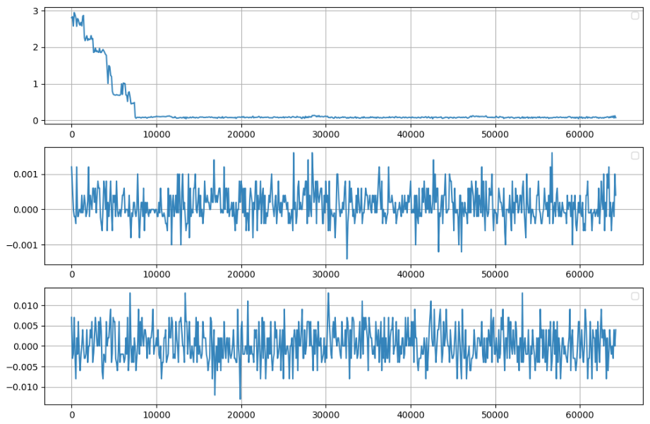
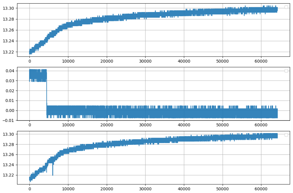
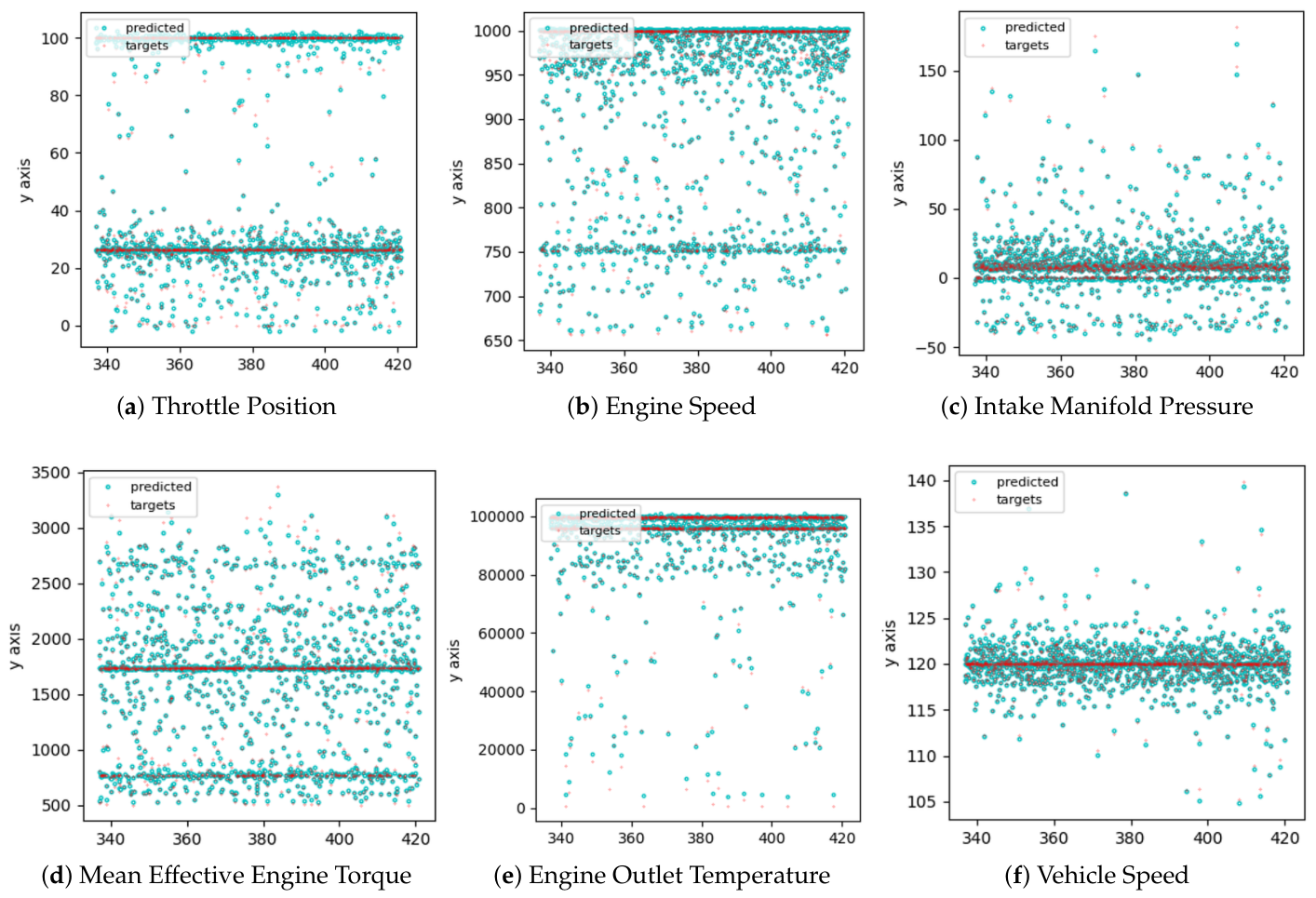
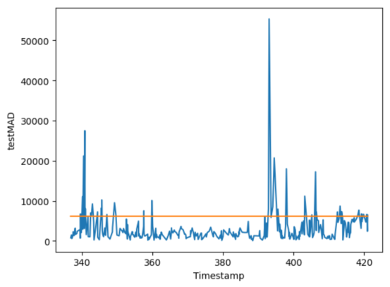
To complement the quantitative results reported in Table 4, Table 5, Table 6 and Table 7, the detection behavior of the ANN-DAE model in the HIL case study is illustrated in Figure 8, Figure 9 and Figure 10.

Figure 8 compares the predicted and target values of the six selected signals over the evaluated test segment. The predictions closely follow the targets across the distinct operating levels of the throttle position and engine speed signals, and the reconstruction quality remains stable for signals with strongly different magnitudes and dynamics, ranging from the intake manifold pressure to the vehicle speed.

Figure 9 presents the mean absolute deviation (MAD) of the reconstruction over the same segment together with the detection threshold. The reconstruction error remains below the threshold during normal operation, whereas pronounced exceedances occur at approximately $t=340$ s and $t=393$ s, where the injected sensor faults distort the measured signals; the largest deviation exceeds the threshold by almost an order of magnitude.

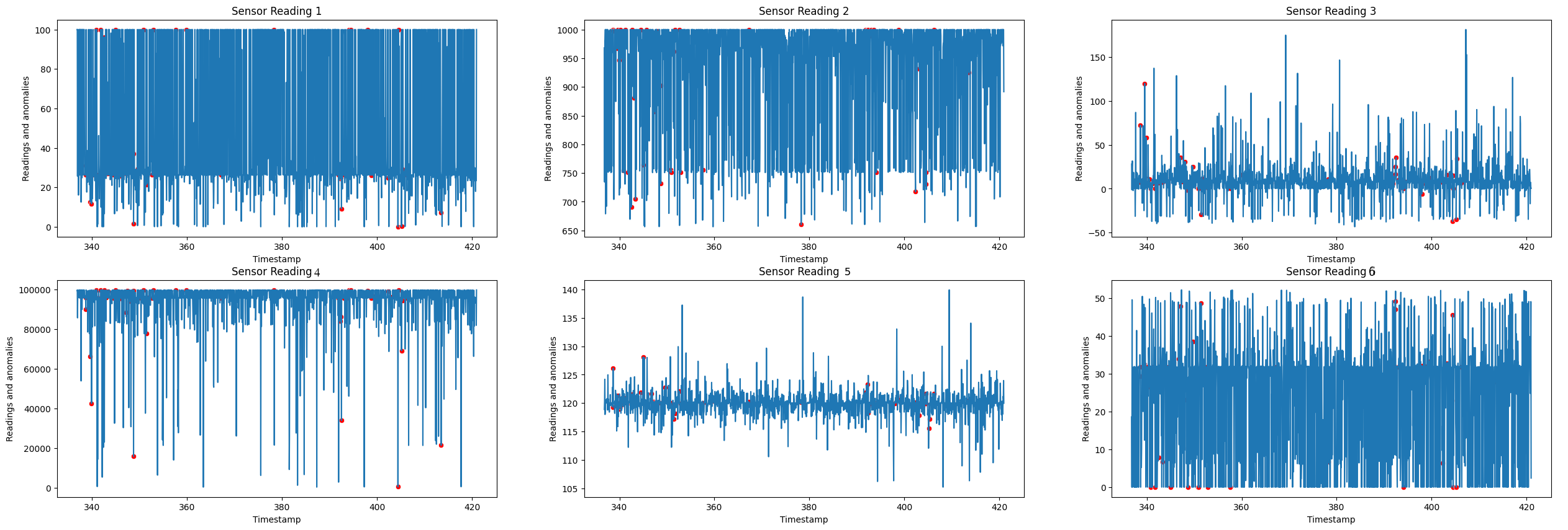
Figure 10 overlays the detected anomalies on the underlying sensor readings. The flagged samples concentrate on physically implausible values, including saturated throttle position readings, abrupt engine speed drops, and isolated outliers in the intake manifold pressure. This confirms that the threshold exceedances in Figure 9 correspond to localized signal distortions rather than to normal operating transitions.

5.2. Performance of the Denoising Autoencoder with Real Test Drive Recordings

5.2.1. Reconstruction Performance

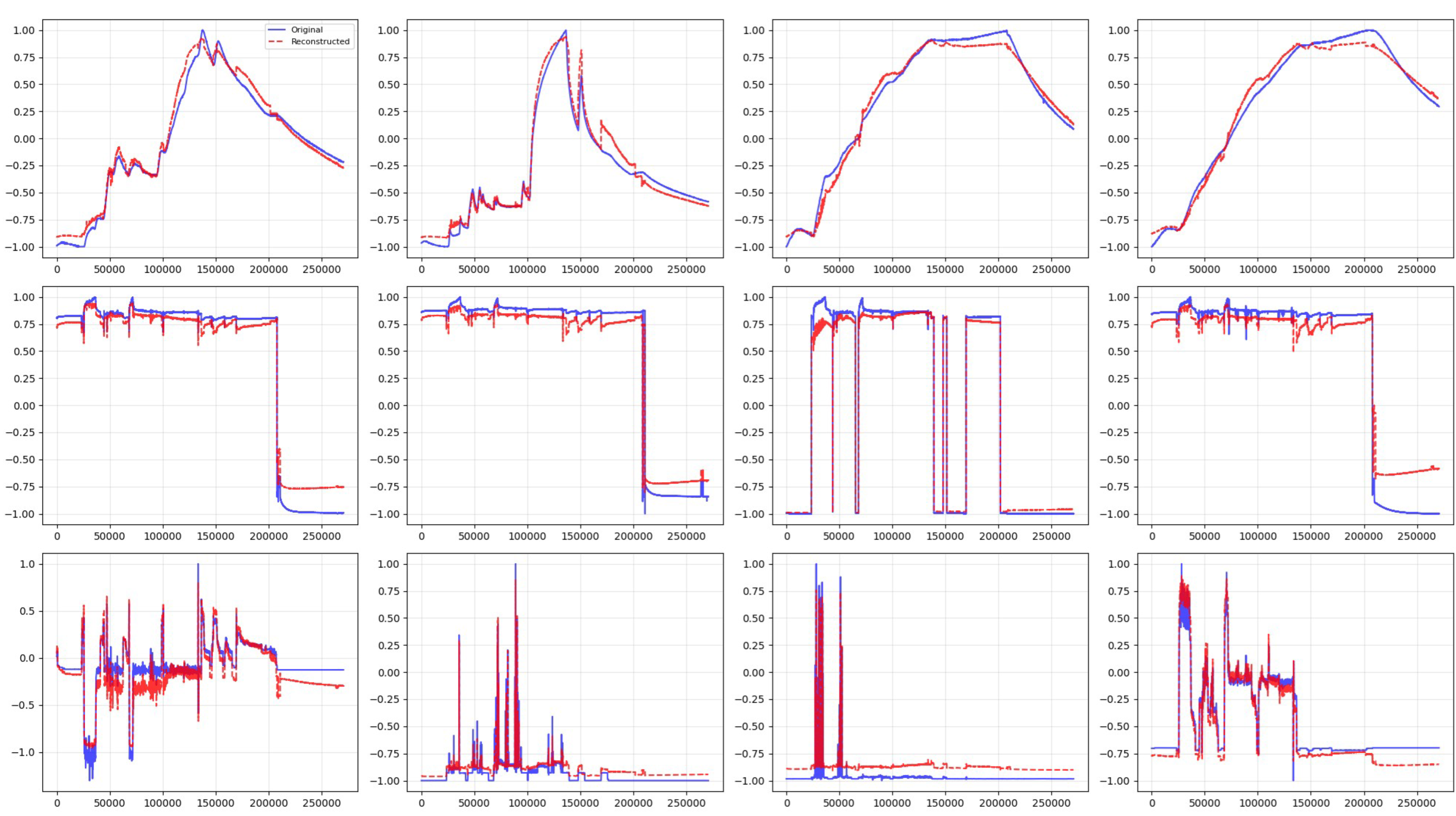
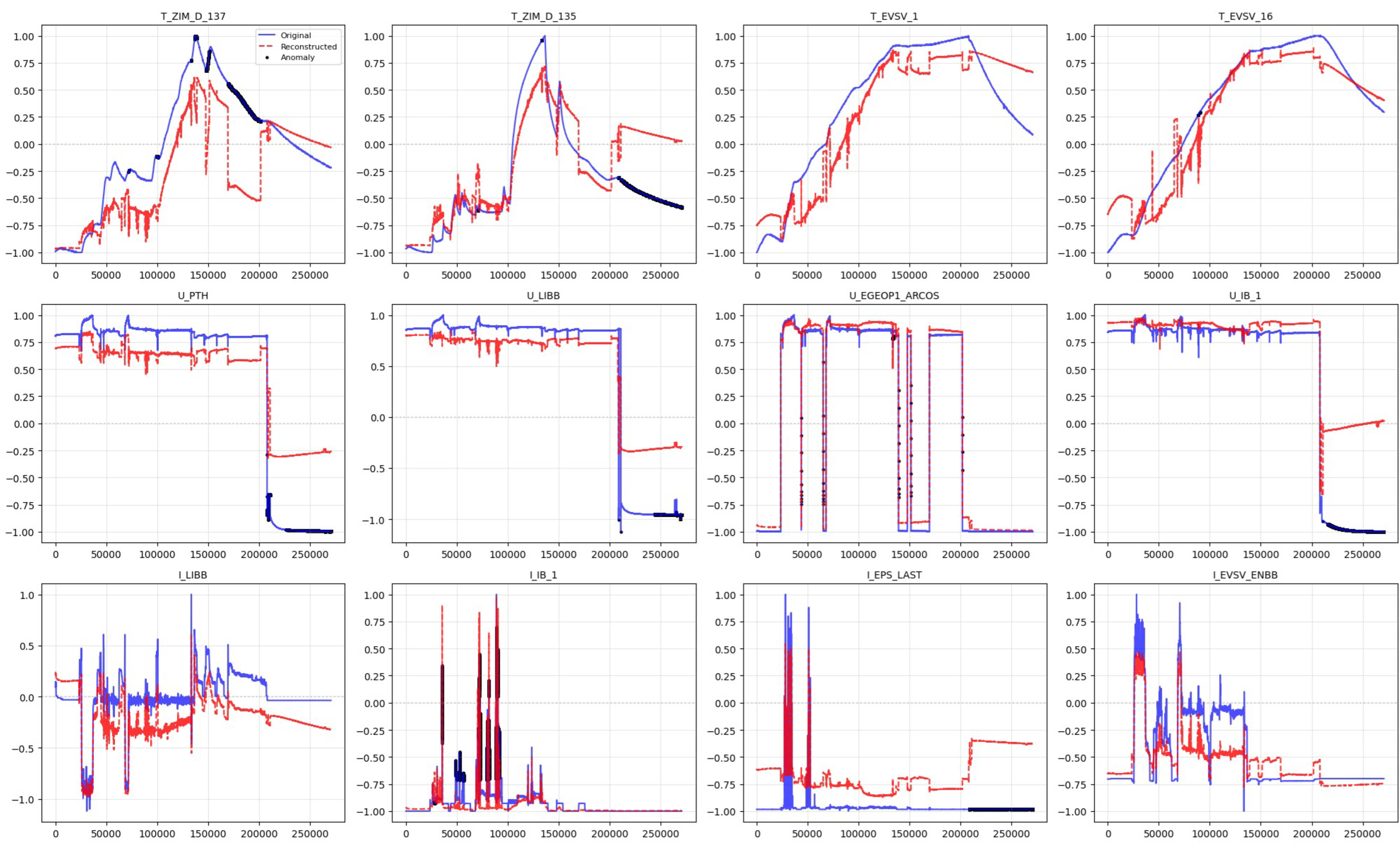
After performing the preprocessing phase, the performance of the DAE was evaluated using real-world measurement data. These measurements were collected during vehicle test drives under various operating and environmental conditions. The model’s reconstruction capability was evaluated using both healthy and faulty data. As demonstrated in Figure 11, the model’s reconstruction performance, employing fault-free operational data, substantiates the efficacy of the proposed architecture in accurately replicating the behavior of the designated signals. In particular, the reconstruction process successfully captures both increased and decreased ranges observed in current measurements with high variance, e.g., for the electric battery and power steering signals. Nevertheless, an analysis of the signal categories reveals that electrical signals demonstrate the highest degree of operational variability during standard vehicle operation.

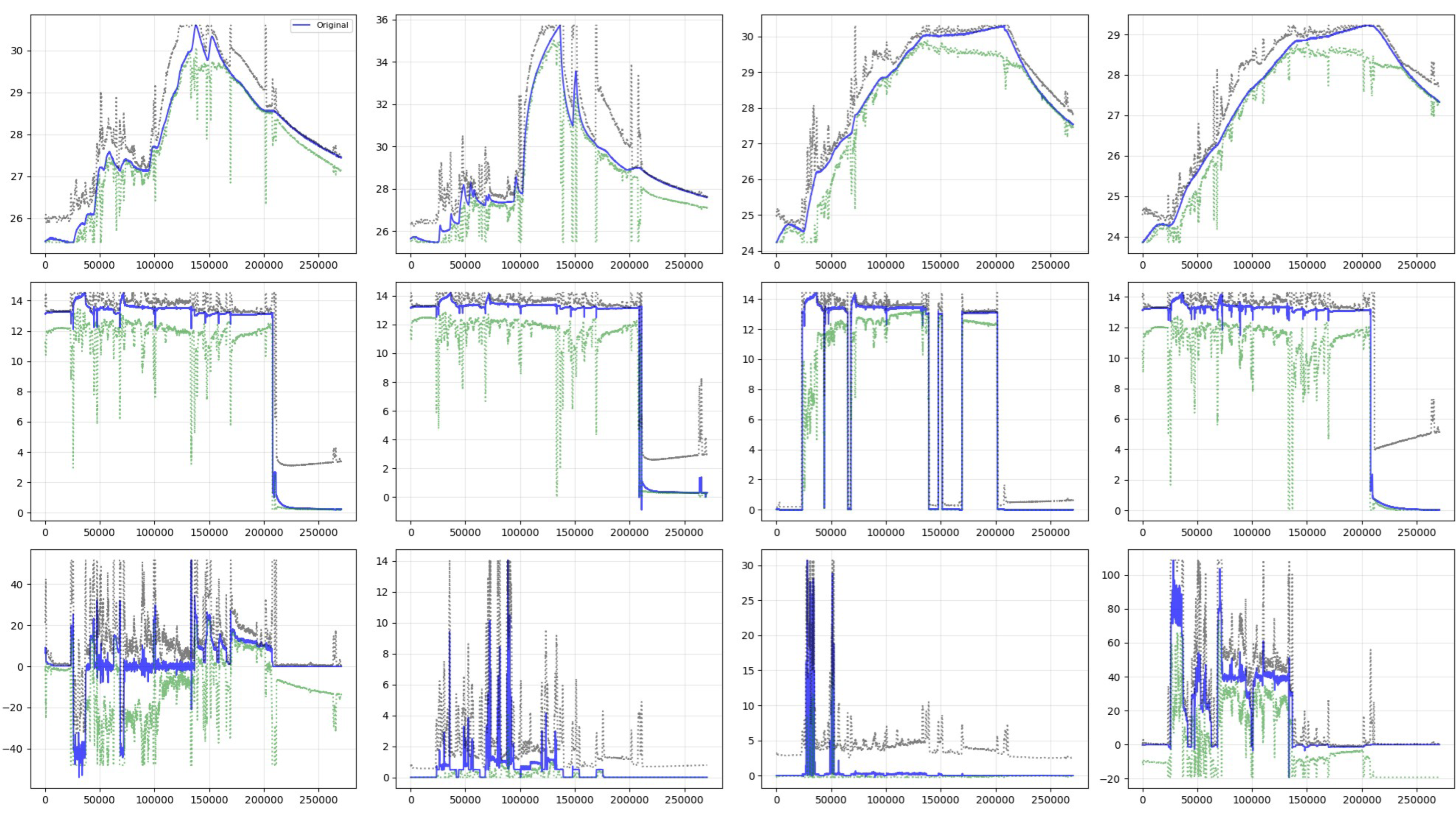
Figure 12 illustrates the reconstruction boundaries that are associated with the adaptive thresholding mechanism, by which the MSE remains minimal in relatively stable signal regions where the signal behavior exhibits limited variation. On the other hand, by increasing the noise in the signal, the distance between the reconstructed output and the upper and lower threshold boundaries becomes significantly larger. By doing so, the ability of the adaptive thresholding mechanism to dynamically respond to local signal variability can be confirmed.

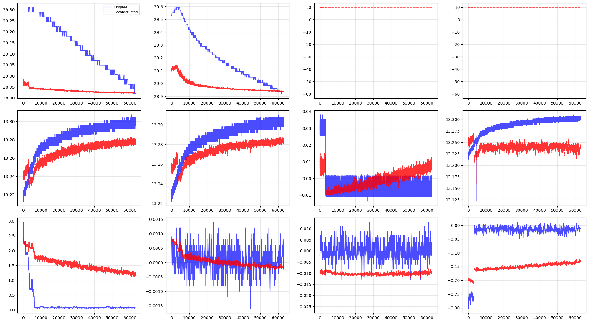
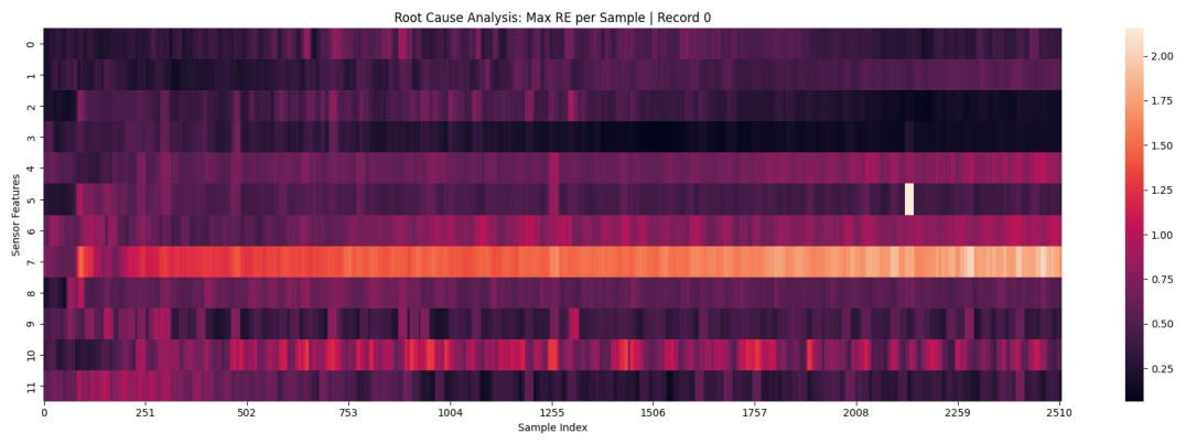
To verify the effectiveness of the proposed DAE in the fault detection process, the model is tested using faulty measurements containing localized anomalies. As can be seen in Figure 13, the anomaly within the control module under the foot pedal assembly is illustrated. Despite the fact that the physical fault is restricted to these individual modules, the reconstruction behavior reveals the propagation of the anomaly across multiple correlated signals. Therefore, it can be concluded that the autoencoder learns nonlinear interdependency among the twelve selected automotive features, resulting in the propagation of reconstruction deviations through the latent representation.

Figure 14 and Figure 15 illustrate the anomaly detection results, i.e., detection of transient spike anomalies within the measured signals. In this case, the adaptive threshold associated with signal 6, corresponding to the 12 V battery voltage measurement, fails to fully contain the abnormal spike behavior. As a result, the proposed framework classifies the event as faulty and reports it as a potential abnormal condition. The obtained results demonstrate the superiority of the adaptive reconstruction-based approach in identifying safety-critical anomalies that may remain undetected when using conventional static-threshold methodologies.

The implementation results indicate a clear dominance of correctly classified samples, whereas the number of false-positive and false-negative predictions remains comparatively limited. Furthermore, the quantitative evaluation metrics summarized in

Table 9. Fault detection performance of ANN-DAE.

Metric	Value
Precision	0.9063
Recall	0.9819
F1-score	0.9391
Accuracy	0.9688

confirm the performance of the proposed model. More specifically, the overall classification accuracy reflects reliable performance across the complete signal set with an F1-score of 0.9391. Furthermore, the high recall value demonstrates the capability of the model to successfully identify the majority of anomalous events.

5.2.2. Performance Comparison with Fixed Thresholding

To demonstrate the effectiveness of the proposed adaptive thresholding mechanism, the model performance was evaluated using a fixed threshold derived from the distribution of reconstruction errors in the training dataset. In this case, the fixed-threshold approach applies a constant decision boundary without taking into account local temporal fluctuations in the signal behavior.

This comparison is conducted using the ANN-DAE model, which was selected as the deployment architecture based on the results reported in Section 5. Since the observed degradation stems from the constant decision boundary rather than from the reconstruction network, a comparable effect is expected for the remaining architectures.

As shown in Figure 16, the threshold limits remain constant over time, even with changing signal variance or operating dynamics.

Table 10. Performance metrics using a fixed threshold.

Metric	Value
Precision	0.5407
Recall	0.5459
F1-score	0.2705
Accuracy	0.2708

shows the results of the quantitative evaluation. It can be observed that anomaly detection performance decreases significantly when using global fixed thresholds. Specifically, the number of detected anomalies increases significantly, leading to a large number of false-positive classifications and a sharp decline in overall accuracy as well as the F1 score. The low values for precision and recall indicate that the model incorrectly classifies a large portion of normal signal behavior as anomalous.

The reason behind this degradation is the highly dynamic nature of automotive measurements under real-world conditions. Specifically, the current and voltage signals exhibit substantial operational fluctuations even under healthy conditions. As a result of applying fixed thresholds, the DAE is unable to adapt to local signal characteristics and therefore incorrectly interprets normal high-variance behavior as a faulty state. In our study, the fixed threshold was identified using the highest 0.1% of reconstruction error values obtained from the training data. Therefore, the propagation of reconstruction deviations between correlated signals amplifies the number of false-positive detections. The comparison results of applying both kinds of thresholding mechanisms demonstrate that fixed-threshold strategies are unsuitable for multivariate automotive time-series analysis. On the other hand, the adaptive thresholding mechanism dynamically adjusts to local signal behavior. This, in turn, leads to significantly improved overall anomaly detection performance.

5.2.3. Performance Analysis Based on Threshold Window Size

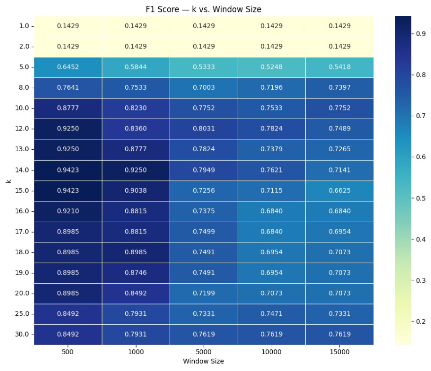
To investigate the robustness of the proposed model, the relationship between the threshold window size, the sensitivity factor k, and the resulting F1-score is analyzed in this section. Figure 17 shows the variation in the F1-score for different combinations of window sizes and threshold sensitivity values.

The window size represents the number of neighboring datapoints considered during the computation of the local moving average and local standard deviation. It is worth noting that the local statistics directly influence the interpretation of reconstruction errors and consequently affect the fault detection sensitivity.

The selection of both parameters follows explicit principles rather than unconstrained tuning. The window length is bounded from below by the number of samples required for stable estimation of the local mean and standard deviation, and from above by the requirement to follow manoeuvre-level signal dynamics; at the 100 Hz sampling rate, windows of 500 to 1000 samples (5 to 10 s) satisfy both constraints. The sensitivity coefficient k compensates for the small local standard deviation of the smoothed reconstruction errors in stable regions and is selected at the performance plateau between k = 15.0 and k = 16.0, where false-positive and false-negative detections balance. The grid analysis in Figure 17 serves as empirical verification of these principles.

The implementation results exhibit a reduction in overall performance by large window sizes. Due to the fact that the automotive signals exhibit highly dynamic variations, smaller windows provide a more precise local context for reconstruction-error evaluation. On the other hand, large temporal windows can excessively smooth local fluctuations. This, in turn, leads to a reduction in the ability of the framework to differentiate between legitimate operational changes and faults. Furthermore, the results indicate that the optimal sensitivity region for the parameter k is illustrated between $15.0$ and $16.0$. Within the mentioned range, the adaptive threshold shows an effective balance between false-positive and false-negative detections. Furthermore, lower values can generate excessive sensitivity to normal signal jitter, whereas larger values permit certain anomalies to remain undetected.

5.2.4. Performance Analysis Based on Noise Injection

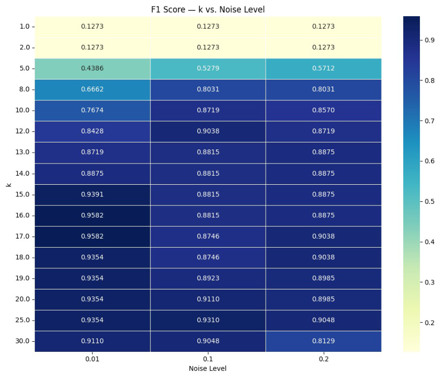
The robustness evaluation of the DAE model against several levels of noise is illustrated in Figure 18. As can be seen, the model performance in terms of the F1-score with respect to the threshold sensitivity parameter k and different levels of injected training noise is illustrated.

It can be observed that increasing the level of the added noise leads to a decrease in the final F1 score compared to the baseline configuration. The rationale behind this phenomenon can be attributed to the distinctive characteristics exhibited by the anomalies present within the MDF4 dataset. It is important to note that the majority of the recorded anomalies consist of a very limited number of erroneous measurements per signal. Consequently, the augmentation of noise levels during training causes the model to interpret abrupt signal fluctuations as normal background noise rather than actual anomalies. This predicament assumes particular significance in the context of contemporary measurements, as sharp transitions can signify either operational alterations or authentic hardware-related defects. It has also been observed that, in the case of high noise levels during training, the encoder generates a latent representation. This phenomenon results in a diminution of the model’s sensitivity to locally confined anomalous events. Consequently, genuine anomalies may be misinterpreted as acceptable noise fluctuations. It can be concluded that lower noise injection levels improve the robustness of the developed anomaly detection framework. It is demonstrated that optimal performance is attained at a noise level of $0.01$ in conjunction with a threshold sensitivity factor of $15.0$.

The F1-scores reported in this analysis quantify the sensitivity of the framework to the threshold factor k and the training noise level. They are obtained over the full parameter grid and do not constitute held-out performance figures; the final evaluation on the held-out test set is reported in Table 9.

5.2.5. Generalization Performance on a Different Vehicle

To demonstrate the generalization of the proposed DAE model, it was evaluated using measurement data collected from a different vehicle under the same driving scenario. The evaluation dataset of the different vehicle comprises both healthy recordings and recordings containing verified anomalous events. Ground-truth labels were derived from the industrial measurement-analysis workflow, in which deviations flagged by the rule-based analysis pipeline are reviewed and confirmed by test engineers. Specifically, the healthy training dataset was curated using existing industrial data-cleaning procedures, previous engineering investigations, expert supervision, and the analysis tools currently employed by IAV for measurement validation. The proposed framework was applied to the unseen recordings without any retraining or fine-tuning, and predictions were generated at the window level using a window size of 1000. Precision, recall, F1-score, and accuracy were subsequently computed by comparing the predicted anomaly windows against the labeled ground truth for each sensitivity value k, as summarized in

Table 11. Model Performance on a new signal for a different vehicle.

Index	k	f1_Score	Precision	Recall	Accuracy
0	1.0	0.200000	0.125000	0.500000	0.250000
1	2.0	0.200000	0.125000	0.500000	0.250000
2	5.0	0.557701	0.648008	0.680556	0.562500
3	8.0	0.681214	0.688811	0.750000	0.708333
4	10.0	0.757576	0.744444	0.805556	0.791667
5	12.0	0.789011	0.777311	0.805556	0.833333
6	13.0	0.833333	0.833333	0.833333	0.875000
7	14.0	0.857058	0.868550	0.847222	0.895833
8	15.0	0.882064	0.910526	0.861111	0.916667
9	16.0	0.882064	0.910526	0.861111	0.916667
10	17.0	0.908571	0.961538	0.875000	0.937500
11	18.0	0.873684	0.950000	0.833333	0.916667
12	19.0	0.873684	0.950000	0.833333	0.916667
13	20.0	0.873684	0.950000	0.833333	0.916667
14	25.0	0.873684	0.950000	0.833333	0.916667
15	30.0	0.873684	0.950000	0.833333	0.916667

.

Compared to the previous vehicle system, the new measurement data originate from different physical vehicle components. Therefore, four temperature signals, four voltage signals, and four current signals were used for the evaluation. Table 11 shows the quantitative evaluation results for a window size of 1000. It can be observed that the proposed framework maintains stable performance in terms of fault detection when applied to unknown signals originating from a different vehicle platform. Specifically, the results show that the highest F1 score achieved is 0.908571, which ensures strong generalization capability across different measurement environments.

5.2.6. Interpretation of Our Results Using Global Permutation Importance and Arcana

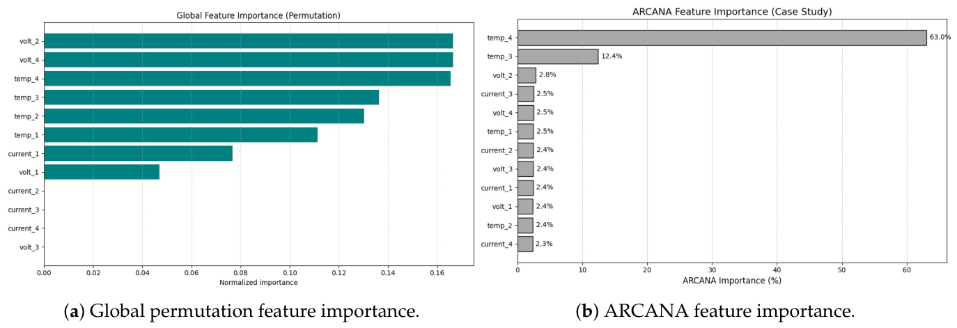
After detecting the faults, it is essential to identify the variables responsible for the detected deviations in order to support maintenance and diagnostic processes. Despite the effectiveness of DAE in detecting abnormal patterns, it does not inherently indicate which features caused the anomaly and how the remaining signals are affected. This issue becomes particularly challenging when analyzing a massive amount of datasets. To address this problem, two interpretation approaches are evaluated in this study, i.e., Global Permutation Importance and Anomaly Root Cause Analysis (ARCANA) [38]. Global Permutation Importance provides an overall estimation of feature relevance. ARCANA, on the other hand, is specifically designed to identify the root causes of individual anomalous events.

Global Permutation Importance is a model-agnostic method used to evaluate feature relevance by randomly shuffling a signal and measuring the resulting increase in reconstruction error [50]. A large increase in the error indicates that the corresponding signal has a significant contribution to the learned representation. As can be seen in Figure 19a, the implementation results on our dataset show that the method correctly identifies volt_2 as an important signal influencing the reconstruction process. However, several additional variables, including volt_4 and temp_4, exhibit similar importance scores, thereby limiting the ability of the method to precisely isolate the actual source of the anomaly.

Unlike conventional reconstruction-error analysis, ARCANA aims at identifying a sparse subset of features responsible for the detected anomaly. The method formulates root-cause identification as an optimization problem through the introduction of a bias vector $x_{bias}$, representing the deviation associated with each feature. The final feature importance is obtained by averaging the absolute values of the bias vector over the anomaly interval and normalizing the results.

As shown in Figure 19b, in contrast to the permutation-based analysis, ARCANA can successfully identify temp_4 and temp_3 as the dominant contributors to the anomaly, assigning importance values of 63.0% and 12.4%, respectively. Since ARCANA does not rely on feature shuffling or temporal variance, it can correctly identify anomalous variables even in the presence of flat signal behavior. Furthermore, the method suppresses the influence of propagated reconstruction errors affecting unrelated signals, thereby providing a clearer explanation of the detected fault.

The two analyzed anomaly cases correspond to events whose root causes were confirmed through engineering inspection within the industrial measurement-analysis workflow. This confirmation provides the reference against which the attribution quality of both methods is assessed. A systematic quantitative evaluation, in which faults with known root causes are injected and the attribution accuracy of each method is measured over a large number of events, is identified as future work.

6. Conclusions

To address the limitations of current rule-based analysis approaches for test-drive recordings, this article proposes a hybrid adaptive DAE-based framework integrating adaptive Gaussian thresholding and XAI techniques for intelligent and transparent fault detection in real and virtual test-drive recordings. Vehicle measurements from real-world test drives and HIL-based virtual test drives, covering varying operating conditions, noise levels, and heterogeneous fault scenarios, were used for model development and evaluation. The results demonstrate robust anomaly detection and strong generalization across both physical and simulated environments. The comparison of DAE variants confirms that the choice of architecture has a central influence on reconstruction and detection performance. ANN-DAE achieved the most stable reconstruction behavior and the highest robustness under noisy conditions, with F1-scores of 0.9391 and 0.9639 on the real and virtual test-drive data, respectively, whereas the recurrent architectures exhibited higher sensitivity to signal disturbances and threshold variations. The adaptive Gaussian thresholding reduces the false-positive rate under varying operating conditions by adjusting the detection thresholds to the statistical behavior of the reconstructed signals, and the integrated XAI techniques enable the interpretation of detection decisions, which is particularly important in safety-critical automotive applications.

Several limitations remain. The evaluation on real test-drive recordings is based on a limited number of held-out windows, and the reported metrics are accompanied by bootstrap confidence intervals rather than repeated training runs; repeated-seed experiments and larger labeled evaluation sets will be addressed in future work. In addition, cross-environment transfer of trained models between HIL-based and real test drives will be investigated using domain adaptation techniques and time-series foundation models, and thresholding strategies based on extreme value theory, which model the tail of the error distribution directly, will be examined to relax the local Gaussian assumption.

References

1. Chakraborty, S.; Al Faruque, M.A.; Chang, W.; Goswami, D.; Wolf, M.; Zhu, Q. Automotive cyber–physical systems: A tutorial introduction. IEEE Des. Test 2016, 33, 92–108. [Google Scholar] [CrossRef]
2. Schindewolf, M.; Guissouma, H.; Sax, E. Analysis and modeling of future electric/electronic architectures for modular vehicles concepts. In 21. Internationales Stuttgarter Symposium: Automobil-und Motorentechnik; Springer: Berlin/Heidelberg, Germany, 2021; pp. 32–46. [Google Scholar]
3. Ebert, C.; Favaro, J. Automotive software. IEEE Softw. 2017, 34, 33–39. [Google Scholar] [CrossRef]
4. Dajsuren, Y.; den Brand, M.v. Automotive software engineering: Past, present, and future. In Automotive Systems and Software Engineering: State of the Art and Future Trends; Springer: Berlin/Heidelberg, Germany, 2019; pp. 3–8. [Google Scholar]
5. Bello, L.L.; Mariani, R.; Mubeen, S.; Saponara, S. Recent advances and trends in on-board embedded and networked automotive systems. IEEE Trans. Ind. Inform. 2018, 15, 1038–1051. [Google Scholar] [CrossRef]
6. Ramesh, S.; Vogel-Heuser, B.; Chang, W.; Roy, D.; Zhang, L.; Chakraborty, S. Specification, verification and design of evolving automotive software. In Proceedings of the 54th Annual Design Automation Conference 2017, Austin, TX, USA, 18–22 June 2017; pp. 1–6. [Google Scholar]
7. ISO 26262-10:2018; Road Vehicles—Functional Safety—Part 10: Guideline on ISO 26262. International Organization for Standardization (ISO): Geneva, Switzerland. Available online: https://www.iso.org/standard/68392.html (accessed on 14 February 2025).
8. Theissler, A. Detecting Anomalies in Multivariate Time Series from Automotive Systems. Ph.D. Thesis, Brunel University School of Engineering and Design, London, UK, 2013. [Google Scholar]
9. Lee, J.W.; Choi, K.Y.; Lee, J.W. Collecting big data from automotive ECUs beyond the CAN bandwidth for fault visualization. Mob. Inf. Syst. 2017, 2017, 4395070. [Google Scholar] [CrossRef]
10. Enisz, K.; Fodor, D.; Szalay, I.; Kovacs, L. Reconfigurable real-time hardware-in-the-loop environment for automotive electronic control unit testing and verification. IEEE Instrum. Meas. Mag. 2014, 17, 31–36. [Google Scholar] [CrossRef]
11. Samuel, S.; Austin, L.; Morrey, D. Automotive test drive cycles for emission measurement and real-world emission levels—A review. Proc. Inst. Mech. Eng. Part J. Automob. Eng. 2002, 216, 555–564. [Google Scholar] [CrossRef]
12. Abboush, M.; Bamal, D.; Knieke, C.; Rausch, A. Intelligent fault detection and classification based on hybrid deep learning methods for hardware-in-the-loop test of automotive software systems. Sensors 2022, 22, 4066. [Google Scholar] [CrossRef] [PubMed]
13. Goina, D.; Hogea, E.; Maties, G. Enhanced Anomaly Detection in Automotive Systems Using SAAD: Statistical Aggregated Anomaly Detection. In Proceedings of the 2024 26th International Symposium on Symbolic and Numeric Algorithms for Scientific Computing (SYNASC), Timisoara, Romania, 16–19 September 2024; IEEE: New York, NY, USA, 2024; pp. 233–241. [Google Scholar]
14. Theissler, A.; Dear, I. An anomaly detection approach to detect unexpected faults in recordings from test drives. In Proceedings of the WASET International Conference on Vehicular Electronics and Safety, Dongguan, China, 28–30 July 2013; Volume 7, pp. 195–198. [Google Scholar]
15. Hernata, F.; Laurent, M.E.; Manalu, S.R.; Shiddiqi, H.A. AI vs. Rule-Based Approaches in Time-Series Anomaly Detection. In Proceedings of the 2025 7th International Conference on Cybernetics and Intelligent System (ICORIS), Mataram, Indonesia, 12–13 September 2025; IEEE: New York, NY, USA, 2025; pp. 1–6. [Google Scholar]
16. Baek, Y.; Jo, M. Adaptive threshold generation for fault detection with high dependability for cyber-physical systems. Appl. Sci. 2018, 8, 2235. [Google Scholar] [CrossRef]
17. Hossain, M.; Rahman, M.; Ramasamy, D. Artificial intelligence-driven vehicle fault diagnosis to revolutionize automotive maintenance: A review. Comput. Model. Eng. Sci. 2024, 141, 951. [Google Scholar] [CrossRef]
18. Al-Zeyadi, M.; Andreu-Perez, J.; Hagras, H.; Royce, C.; Smith, D.; Rzonsowski, P.; Malik, A. Deep learning towards intelligent vehicle fault diagnosis. In Proceedings of the 2020 International Joint Conference on Neural Networks (IJCNN), Glasgow, UK, 19–24 July 2020; IEEE: New York, NY, USA, 2020; pp. 1–7. [Google Scholar]
19. Javed, A.R.; Usman, M.; Rehman, S.U.; Khan, M.U.; Haghighi, M.S. Anomaly detection in automated vehicles using multistage attention-based convolutional neural network. IEEE Trans. Intell. Transp. Syst. 2020, 22, 4291–4300. [Google Scholar] [CrossRef]
20. Davari, N.; Pashami, S.; Veloso, B.; Nowaczyk, S.; Fan, Y.; Pereira, P.M.; Ribeiro, R.P.; Gama, J. A fault detection framework based on lstm autoencoder: A case study for volvo bus data set. In International Symposium on Intelligent Data Analysis; Springer: Berlin/Heidelberg, Germany, 2022; pp. 39–52. [Google Scholar]
21. Hsieh, R.J.; Chou, J.; Ho, C.H. Unsupervised online anomaly detection on multivariate sensing time series data for smart manufacturing. In Proceedings of the 2019 IEEE 12th Conference on Service-Oriented Computing and Applications (SOCA), Taiwan, China, 18–21 November 2019; IEEE: New York, NY, USA, 2019; pp. 90–97. [Google Scholar]
22. Tziolas, T.; Papageorgiou, K.; Theodosiou, T.; Papageorgiou, E.; Mastos, T.; Papadopoulos, A. Autoencoders for anomaly detection in an industrial multivariate time series dataset. Eng. Proc. 2022, 18, 23. [Google Scholar] [CrossRef]
23. Chen, T.; Liu, X.; Xia, B.; Wang, W.; Lai, Y. Unsupervised anomaly detection of industrial robots using sliding-window convolutional variational autoencoder. IEEE Access 2020, 8, 47072–47081. [Google Scholar] [CrossRef]
24. Abboush, M.; Knieke, C.; Rausch, A. GRU-based denoising autoencoder for detection and clustering of unknown single and concurrent faults during system integration testing of automotive software systems. Sensors 2023, 23, 6606. [Google Scholar] [CrossRef] [PubMed]
25. Abboush, M.; Knieke, C.; Rausch, A. Intelligent back-to-back testing with denoising autoencoder-based fault detection and dbscan clustering. Results Eng. 2025, 27, 105900. [Google Scholar] [CrossRef]
26. Fang, Y.; Min, H.; Wu, X.; Lei, X.; Chen, S.; Teixeira, R.; Zhao, X. Toward interpretability in fault diagnosis for autonomous vehicles: Interpretation of sensor data anomalies. IEEE Sens. J. 2023, 23, 5014–5027. [Google Scholar] [CrossRef]
27. Abboush, M.; Ghannoum, E.; Rausch, A. An explainable hybrid deep learning-enabled intelligent fault detection and diagnosis approach for automotive software systems validation. Knowl.-Based Syst. 2025, 334, 114922. [Google Scholar]
28. Hwang, C.; Lee, T. E-SFD: Explainable sensor fault detection in the ICS anomaly detection system. IEEE Access 2021, 9, 140470–140486. [Google Scholar] [CrossRef]
29. Lin, C.; Du, B.; Sun, L.; Li, L. Hierarchical context representation and self-adaptive thresholding for multivariate anomaly detection. IEEE Trans. Knowl. Data Eng. 2024, 36, 3139–3150. [Google Scholar] [CrossRef]
30. Biddle, L.; Fallah, S. A novel fault detection, identification and prediction approach for autonomous vehicle controllers using SVM. Automot. Innov. 2021, 4, 301–314. [Google Scholar] [CrossRef]
31. Namigtle-Jiménez, A.; Escobar-Jiménez, R.; Gómez-Aguilar, J.; García-Beltrán, C.; Téllez-Anguiano, A. Online ANN-based fault diagnosis implementation using an FPGA: Application in the EFI system of a vehicle. Isa Trans. 2020, 100, 358–372. [Google Scholar] [CrossRef] [PubMed]
32. Safavi, S.; Safavi, M.A.; Hamid, H.; Fallah, S. Multi-sensor fault detection, identification, isolation and health forecasting for autonomous vehicles. Sensors 2021, 21, 2547. [Google Scholar] [CrossRef] [PubMed]
33. Kaplan, H.; Tehrani, K.; Jamshidi, M. A fault diagnosis design based on deep learning approach for electric vehicle applications. Energies 2021, 14, 6599. [Google Scholar] [CrossRef]
34. Raveendran, R.; Devika, K.; Subramanian, S.C. Brake fault identification and fault-tolerant directional stability control of heavy road vehicles. IEEE Access 2020, 8, 169229–169246. [Google Scholar] [CrossRef]
35. von Schleinitz, J.; Graf, M.; Trutschnig, W.; Schröder, A. VASP: An autoencoder-based approach for multivariate anomaly detection and robust time series prediction with application in motorsport. Eng. Appl. Artif. Intell. 2021, 104, 104354. [Google Scholar] [CrossRef]
36. Wang, B.; Li, W.; Khattak, Z.H. Anomaly Detection in Connected and Autonomous Vehicle Trajectories Using LSTM Autoencoder and Gaussian Mixture Model. Electronics 2024, 13, 1251. [Google Scholar] [CrossRef]
37. Khanmohammadi, F.; Azmi, R. Time-Series Anomaly Detection in Automated Vehicles Using D-CNN-LSTM Autoencoder. IEEE Trans. Intell. Transp. Syst. 2024, 25, 9296–9307. [Google Scholar] [CrossRef]
38. Rüttgers, A.; Heinisch, P.; Schröder, W.G.; Vogt, M.; Müller, A. Autoencoder-based anomaly root cause analysis for wind turbines. Energy AI 2021, 4, 100065. [Google Scholar] [CrossRef]
39. Jiang, R.; Xue, Y.; Zou, D. Interpretability-Aware Industrial Anomaly Detection Using Autoencoders. IEEE Access 2023, 11, 60490–60500. [Google Scholar] [CrossRef]
40. Basaran, O.T.; Dressler, F. Explainable and Interpretable Deep Contractive Autoencoder for O-RAN Traffic Anomaly Detection. Comput. Netw. 2025, 261, 111145. [Google Scholar] [CrossRef]
41. Zhang, X.; Wang, G.; Chen, Y.; Yang, W. Inter-layer Explainable Variational Autoencoder Model for Multivariate Time Series Anomaly Detection. Eng. Appl. Artif. Intell. 2025, 159, 111585. [Google Scholar] [CrossRef]
42. Abboush, M.; Knieke, C.; Rausch, A. A virtual testing framework for real-time validation of automotive software systems based on hardware in the loop and fault injection. Sensors 2024, 24, 3733. [Google Scholar] [CrossRef] [PubMed]
43. Xue, B.; Zhang, M.; Browne, W.N.; Yao, X. A survey on evolutionary computation approaches to feature selection. IEEE Trans. Evol. Comput. 2015, 20, 606–626. [Google Scholar] [CrossRef]
44. Acharya, U.R.; Fujita, H.; Lih, O.S.; Hagiwara, Y.; Tan, J.H.; Adam, M. Automated detection of arrhythmias using different intervals of tachycardia ECG segments with convolutional neural network. Inf. Sci. 2017, 405, 81–90. [Google Scholar] [CrossRef]
45. Ahmad, S.; Lavin, A.; Purdy, S.; Agha, Z. Unsupervised real-time anomaly detection for streaming data. Neurocomputing 2017, 262, 134–147. [Google Scholar] [CrossRef]
46. Goodman, N.R. Statistical analysis based on a certain multivariate complex Gaussian distribution (an introduction). Ann. Math. Stat. 1963, 34, 152–177. [Google Scholar] [CrossRef]
47. Vincent, P.; Larochelle, H.; Bengio, Y.; Manzagol, P.A. Extracting and composing robust features with denoising autoencoders. In Proceedings of the 25th International Conference on Machine Learning, Helsinki, Finland, 5–9 July 2008; pp. 1096–1103. [Google Scholar]
48. Automotive Simulation Models. Available online: https://www.dspace.com/en/pub/home/products/sw/automotive_simulation_models.cfm#175_26315 (accessed on 11 April 2023).
49. Du, S.; Wan, Y.; Zhang, C.; Zhang, S. Anomaly root cause analysis for wind turbines based on denoising autoencoder and sparse estimation. In Proceedings of the 2023 IEEE 12th Data Driven Control and Learning Systems Conference (DDCLS), Xiangtan, China, 12–14 May 2023; IEEE: New York, NY, USA, 2023; pp. 449–454. [Google Scholar]
50. Altmann, A.; Toloşi, L.; Sander, O.; Lengauer, T. Permutation importance: A corrected feature importance measure. Bioinformatics 2010, 26, 1340–1347. [Google Scholar] [CrossRef] [PubMed]
Figure 1. Proposed framework for fault detection based on adaptive ANN-DAE and XAI techniques.
Electronics 15 02723 g001
Figure 2. Proposed DAE architecture for fault detection.
Electronics 15 02723 g002
Figure 3. Current signal profiles illustrating peaks and load fluctuations during operational cycles.
Electronics 15 02723 g003
Figure 4. Voltage signal distributions across varying load conditions, demonstrating the baseline electrical stability of the system.
Electronics 15 02723 g004
Figure 5. Temperature measurements exhibiting slow-moving thermal trends and steady-state operational plateaus.
Electronics 15 02723 g005
Figure 6. Smoothed moving-average profiles of the selected signals, grouped by physical domain: (top) current signals (I), (middle) voltage signals (U), and (bottom) temperature signals (T).
Electronics 15 02723 g006
Figure 7. HIL-based virtual test drives for real-time validation.
Electronics 15 02723 g007
Figure 8. Comparison between predicted and target values for the six selected signals using the proposed model.
Electronics 15 02723 g008
Figure 9. Mean absolute deviation (MAD) of the reconstruction over the evaluated test segment. The blue curve shows the per-window reconstruction MAD, and the horizontal orange line marks the detection threshold; windows whose MAD exceeds this threshold are flagged as anomalous.
Electronics 15 02723 g009
Figure 10. Detected anomalies (marked in red) overlaid on the selected sensor readings of the HIL test segment.
Electronics 15 02723 g010
Figure 11. Reconstruction performance on healthy data.
Electronics 15 02723 g011
Figure 12. Upper and lower adaptive threshold boundaries on healthy data for the twelve selected signals. In each panel, the blue solid line is the original signal, the grey dotted line is the upper threshold boundary, and the green dotted line is the lower threshold boundary. The boundaries widen in regions of higher signal variability and tighten in stable regions, reflecting the local adaptation of the thresholding mechanism to the signal behaviour.
Electronics 15 02723 g012
Figure 13. Reconstruction performance on faulty data.
Electronics 15 02723 g013
Figure 14. Detection of a transient spike anomaly for the twelve selected signals. In each panel, the blue solid line is the original signal, the grey dotted line is the upper threshold boundary, and the green dotted line is the lower threshold boundary. The signals remain within the threshold band during normal operation, whereas the spike in the 12 V battery voltage signal exceeds the upper boundary and is therefore flagged as a faulty event.
Electronics 15 02723 g014
Figure 15. Heatmap of the reconstruction with a faulty recording.
Electronics 15 02723 g015
Figure 16. Reconstruction performance using a fixed threshold.
Electronics 15 02723 g016
Figure 17. F1-score based on the window size and factor k.
Electronics 15 02723 g017
Figure 18. F1-score based on the noise level and factor k.
Electronics 15 02723 g018
Figure 19. Comparison of feature importance obtained using global permutation importance and ARCANA.
Electronics 15 02723 g019