

Article

RASC: Region-Aware Self-Calibration for Dense 2D Sensor Arrays
College of Smart Materials and Future Energy, Fudan University, Shanghai 200433, China
*
Author to whom correspondence should be addressed.
Electronics 2026, 15(12), 2724; https://doi.org/10.3390/electronics15122724
Submission received: 5 May 2026 / Revised: 8 June 2026 / Accepted: 16 June 2026 / Published: 19 June 2026
(This article belongs to the Special Issue Feature Papers in Networks: 2025–2026 Edition)

Abstract

Bipolar junction transistor (BJT)-based 2D temperature-sensor arrays are factory-calibrated to ±0.1 °C, but post-deployment thermal and mechanical stresses drift their per-sensor gain–offset parameters by an order of magnitude, and in-lab recalibration is impractical. We present RASC (Region-Aware Self-Calibration), a five-stage algorithm that decomposes the global ill-posed problem into local cluster-level problems, runs robust alternating estimation (trimmed-mean field reconstruction + Huber iteratively reweighted least squares (IRLS)) inside each cluster, and reconciles overlapping estimates by linear consensus on the cluster-overlap graph with provable exponential convergence. On 7632 frames from a deployed 16 × 16 array exhibiting ≈5× factory-spec non-uniformity, RASC cuts the locally non-smooth fixed-pattern residual by 71 ± 5% (10-fold cross-validation (CV)), reducing this residual to a level comparable to the ±0.1 °C factory specification (as assessed by local-smoothness residual metrics, not independent absolute-temperature validation) while perturbing the calibrated field by only 0.041 °C RMSE; reduction concentrates at the edges (78% vs. 55% interior). In simulations on 8 × 8 to 32 × 32 arrays, RASC matches an oracle centralised extended Kalman filter (EKF) within 0.10 °C with ≈4× lower bandwidth. The real-data evaluation is a single-deployment proof of concept on one array and one host PCB; broader, longitudinal validation remains future work.

1. Introduction

Dense 2D temperature-sensor arrays that use the temperature coefficient effect of bipolar junction transistors (BJTs) are widely employed in the thermal monitoring of power electronics, battery packs and industrial process equipment. Each pixel is based on the temperature dependence of the base-emitter voltage V_BE, which is a well-known physical phenomenon and the basis of modern BJT-based temperature sensors achieving sub-0.1 °C inaccuracy after factory calibration [1,2]; thus, it has been factory-calibrated using a traceable temperature reference to within ±0.1 °C of the production temperature. Although the array has been added to the target system, the three deployment-specific stresses affect each die differently: (i) Reflow soldering thermal cycling introduces residual mechanical stress at the V_BE junction, thereby changing both gain and offset. (ii) The local PCB heat-dissipation path varies across the array, and edge pixels lose heat asymmetrically through nearby copper pours, mounting holes or chassis contacts, resulting in spatially structured biassing readings. (iii) Packaging stress, humidity ingress and slow electromigration further perturb the V_BE over the course of several months of operation. The result of the above is that the deployed array no longer meets the ±0.1 °C factory specification; that is, the per-sensor affine parameters (a_i, b_i) have drifted from their stored factory values, and taking each module offline for laboratory recalibration against a temperature reference is unfeasible in a fielded system.
The recorded data analysed in this paper show this drift directly. Although the device was factory-calibrated to ±0.1 °C, the deployed 16 × 16 array has a peak-to-peak spatial non-uniformity of 0.569 °C in the steady-state field, approximately five times higher than the factory specification. Since the underlying thermal scene is locally smooth by physical argument, this excess non-uniformity must be due to post-deployment drift in (a_i, b_i). Online recalibration would address this drift without taking the array out of service. The technical difficulty is that the in situ setting provides no labelled inputs; the actual thermal field x(p, t) at each sensor location is unknown, no controlled stimulus is applied, and any algorithm must rely only on the structural prior that the physical field is locally smooth. Since the field is unobserved, any recovered estimate of (a_i, b_i) is only identifiable up to a global linear shift unless a small fraction of the nodes provides external anchoring. We therefore study a realistic scenario where a small reference set R, such that |R|/n ≪ 1, can retain accurate factory metadata (e.g., a small number of factory-traceable reference sensors physically isolated from the deployment stress, or sensors that have been individually re-verified at maintenance intervals), and the remaining nodes are recalibrated based on co-observed data alone.
Existing approaches fall into three categories. (a) Classical centralised non-uniformity correction (NUC) was first introduced for infrared (IR) focal-plane arrays (FPA), assumes a uniform stimulus or scene-based motion to recover per-sensor parameters [3,4], and although the two-point and constant-statistics ideas can be extended to any factory-calibrated sensor grid, an external excitation is still required that is not available in our sealed-deployment scenario. (b) Distributed self-calibration in wireless sensor network (WSN) literature [5,6] estimates relative parameters through pairwise consistency at the edges, but generally requires either a known stimulus or restrictive parametric assumptions about the field. (c) Recent learning-based calibration methods [7,8] achieve high accuracy but are limited by large training corpora and per-deployment fine-tuning, and offer no convergence guarantees under unseen conditions.
RASC (Region-Aware Self-Calibration) is a new five-stage algorithm proposed for this online recalibration mode. RASC is entirely unsupervised, does not assume a parametric field model, runs natively in a decentralised manner when desired, and provides explicit convergence guarantees. Generally speaking, the global ill-posed problem is divided into a sequence of local well-posed problems by dividing the array into overlapping spatial clusters, where the physical field is assumed to be well-approximated by a single common signal. In each cluster, we run a robust alternating estimation process that alternates between (i) reconstructing the local field using the trimmed mean of calibrated readings and (ii) re-fitting the (a, b) parameters of each sensor via iteratively re-weighted least squares (IRLS) with Huber loss; we refer to this loop as alternating robust estimation rather than expectation-maximisation because the field-reconstruction step is a deterministic robust estimator rather than a conditional expectation under a probabilistic model. Sensors that are included in multiple cluster estimations across the clusters perform linear consensus iterations to resolve the discrepancies, and the convergence speed is exponential and determined by the algebraic connectivity λ_2(L_C) of the cluster-overlap graph. We emphasise that the novelty of RASC lies not in any single estimator—trimmed-mean field reconstruction, Huber IRLS and linear consensus are individually classical—but in their principled integration into one unsupervised, side-information-free pipeline adapted to the statistics of dense BJT temperature-sensor arrays, together with the accompanying convergence and breakdown-point analysis and the validation on real deployed hardware.

1.1. Contribution

The main contents of this paper are as follows:
  • A principle-based combination of region-based decomposition, robust local estimation and inter-cluster consensus in a five-stage algorithm with deterministic, side-information-free cluster-head election, and explicit convergence properties of all three components are provided.
  • Three convergence and robustness results adapted to the cluster-overlap setting: (Theorem 1) per-cluster alternating-estimation monotone descent under cluster Hessian positive-definiteness; (Theorem 2) inter-cluster consensus exponential rate ρ ≤ 1 − αλ_2(L_C), specialising the classical Olfati-Saber-Murray result [9] to the cluster-overlap graph; (Theorem 3) finite-sample replacement breakdown of the trimmed-mean field reconstruction.
  • A total of three array scales were used for comprehensive simulation studies, with 30 independent runs each, and RASC was compared against an oracle centralised extended Kalman filter (EKF) and a faithful re-implementation of the Bychkovskiy–Megerian–Estrin–Potkonjak (BMEP) edge-pairwise calibration baseline [5], as well as four simpler baselines (uncalibrated, temporal smoothing, pairwise differential, and median spatial filter). Robustness and Sensitivity are tested with combined node failure and packet loss, and analysed along η, α and N_min.
  • A real-sensor study of 7632 frames of data from a 16 × 16 BJT-based temperature array on a host PCB showed that the factory ±0.1 °C specification had been exceeded post-deployment (measured a peak-to-peak non-uniformity (NU) of 0.569 °C and about five times the factory specification). RASC is applied to the in situ readings, and the locally non-smooth fixed-pattern residual is reduced by 71 ± 5% (10-fold cross-validation); thus, by this residual metric the array approaches the original factory specification (an inference from local-smoothness residuals, not an independent absolute-accuracy measurement), and only a 0.041 °C RMSE increase in the calibrated field is observed. The decrease is relatively large at the edges of the array (78% vs. 55% in the middle), and this matches the experimental observation.
  • An honest discussion of identifiability: Why per-sensor (a, b) recovery is degenerate along a one-dimensional gauge in narrow-range fields even when the reconstructed field is good, and the mitigation offered by reference anchoring, as well as a discussion of when the gauge ambiguity is practically significant.

1.2. Paper Organisation

Section 2 surveys the Related Work. Section 3 formally defines the sensor model and identifies the identifiability conditions. Section 4 is the RASC algorithm’s five-step procedure. Section 5: Theoretical Analysis is presented here. Section 6 is the Monte Carlo simulation results. Section 7 is the real-sensor evaluation, and the limitation of a single dataset is explicitly stated. Section 8 covers deficiencies and extensions, and Section 9 presents the conclusion.

2. Related Work

2.1. Centralised Non-Uniformity Correction

Non-uniformity correction has a long history in dense IR focal-plane array imaging [10]. The original shutterless NUC system was introduced by Narendra and Foss [11], and the linear theory of two-point NUC was subsequently developed by Perry and Dereniak [12]. Two-point and multi-point factory NUC are still the main industrial methods [3], and they produce a per-pixel (a, b) lookup table calibrated with external references. The structure of fitting affine parameters with one or more known stimuli applies to all factory-calibrated sensor grids, including the calibrated temperature-sensor array mentioned in Section 7; however, in all cases, controlled stimuli are needed that cannot be re-applied in the field without special hardware. Scene-based NUC algorithms, such as constant-statistics [13] and inter-frame registration [4], relax this requirement but converge slowly when the scene motion is small and degrade if there is stationary structure in the scene that aligns with fixed-pattern noise. More recent work extends classical scene-based NUC with principal-component decomposition [14] and median-ratio statistics on neighbour pixels [15], and explores deep recurrent and convolutional neural network (CNN)-based estimators of fixed-pattern noise; these methods, however, retain the FPA-imaging assumption of inter-frame translational scene motion. RASC is complementary to these scene-based methods: it operates in a single static or slowly varying scene and exploits the spatial smoothness of the background field rather than temporal scene motion or external stimuli.

2.2. Distributed Calibration in WSNs

Bychkovskiy et al. [5] proposed post-deployment recalibration by pairwise relative parameter estimation at the edges and then global consistency optimisation, and showed accurate offset recovery for light sensors. Whitehouse and Culler [16] proposed a related framework of calibrated reference exposures broadcast via the network. Both approaches share the three properties we also adopt: no central fusion, no parametric field model, and no labelled data. Compared with the above classical methods, RASC offers (i) a multi-cluster decomposition (instead of dyadic edge-by-edge estimation) that better utilises dense 2D structure; (ii) explicit robustness to outlier sensors via trimmed mean and Huber IRLS; (iii) a convergence rate certificate ρ ≤ 1 − αλ_2(L); and (iv) validation on a 256-sensor dense array. Subsequent extensions [6,17] use Gaussian process priors on the field and achieve higher accuracy at the expense of explicit kernel specification; we deliberately avoid such priors to retain field-model-free operation. The most closely related contemporary work is the cluster-based drift self-calibration of Ahmad [18], which partitions low-cost sensor networks and applies statistical drift screening with inverse-distance weighting (rather than per-cluster robust parameter recovery), and the trust-based consensus framework of Mahajan and Helbing [19], which weighs neighbour contributions by reliability scores for PM2.5 sensor calibration; both motivate the cluster-and-consensus combination that RASC formalises with explicit convergence and breakdown-point guarantees.

2.3. Robust and Median-Based Estimation

Trimmed-mean and median estimators are well-known robust statistics, and the famous breakdown-point analysis was first introduced by Huber [20] and Hampel [21]. Theorem 3 specialises these classical bounds to the per-cluster setting and connects them to the choice of η in consistency screening. median absolute deviation (MAD)-based screening at the neighbourhood level is in line with practice for fault detection [22], and RASC is novel in that it has been integrated with cluster-head elections and the resulting computation–communication trade-off.

2.4. Consensus Algorithms

Linear distributed averaging and its convergence properties are well-known [9,23]. Olfati-Saber and Murray have shown that the rate of convergence is determined by the second-smallest Laplacian eigenvalue. We use this result in the cluster-overlap graph instead of the sensor proximity graph, and it has good algebraic connectivity even for a large number of arrays due to the overlap geometry. Recent empirical studies confirm that algebraic connectivity remains the dominant predictor of consensus convergence rate across diverse network classes [24], supporting our use of the cluster-overlap Laplacian as the design parameter for Stage 5.

2.5. Learning-Based Calibration

Recently, works [7,8] have applied graph neural networks (GNN) and self-supervised representation learning to sensor calibration. These learning-based approaches outperform model-based pipelines when the training data closely matches the deployment environment, but they require per-application data collection and offer no analytical convergence guarantees for out-of-distribution inputs. We do not include a GNN baseline in our quantitative comparison; a proper GNN evaluation would require training data from a population of similarly deployed arrays, which we do not have for this BJT-on-PCB system, and using such data would shift the comparison from “calibration accuracy” to “data-collection effort”, thereby confounding the methodological question we aim to answer. The classical model-based BMEP baseline [5] in Section 6.5 serves as a suitable reference point for the no-training, no-learning-curve regime that RASC aims to achieve. More broadly, the approach connects to several active and recent lines of work. Post-deployment drift compensation reconstructs each sensor’s slowly varying response from its own signal statistics [25], the regime RASC targets, although RASC additionally exploits the dense spatial structure of the array rather than treating each sensor in isolation. Machine-learning-based in-field calibration of low-cost sensor arrays attains high accuracy by training data-driven correction models [26]; RASC instead uses no per-deployment training corpus and recovers the calibration directly from co-observed data. Distributed consensus estimation over sensor networks recovers state or parameters by iterative agreement among neighbouring nodes [27], paralleling the linear-consensus stage of RASC, which augments it with trimmed-mean and Huber-IRLS robustness so that a fraction of corrupted sensors cannot dominate the estimate. Relative to all three lines, RASC remains unsupervised, field-model-free and equipped with explicit convergence and breakdown-point guarantees.

3. Problem Formulation

3.1. Sensor Model

An array of n sensors has been arranged in a planar grid (or quasi-grid). Sensor i at position p_i ∈ ℝ2 produces a measurement at discrete time t given by
y_i(t) = a_i x(p_i, t) + b_i + ε_i(t),       i = 1, …, n,
where x(p, t) is the unobserved physical field, (a_i, b_i) are the per-sensor gain and offset, and ε_i(t) ~ N(0, σ_i2) is i.i.d. measurement noise. We set:
  • (A1) Local field smoothness: There is a length scale ℓ such that, in any disc of radius r ≤ , the field x(·, t) is well-approximated by a single common signal x ¯ (t).
  • (A2) Bounded heterogeneity: a_i ∈ [a_min, a_max] with 0 < a_min, and |b_i| ≤ B for a finite B; both are constant over the calibration time horizon T.
  • (A3) Reference anchoring: A subset R ⊂ {1,…,n} of size |R| = ρn, where ρ≪1 (e.g., 5%), consists of known (a_i, b_i) for i ∈ R.
Assumption (A1) is typical in the literature on spatial statistics, and for the temperature data analysed in Section 7, it holds with ℓ ≈ 4 sensors at our sampling rate. Assumption (A3) is needed for global identifiability; without anchoring, any consistent solution can be transformed into another by scaling and shifting, i.e., a_i ← κ a_i, b_i ← κ b_i + c for any (κ, c).

3.2. Identifiability

Let X(t) ∈ ℝM be the trimmed-mean field reconstruction over T frames. The conditional least-squares problem for sensor j given the reconstructed field is well-posed if and only if the temporal range Δx_j of X(t) at sensor j is positive. The asymptotic covariance of (â_j, b ^ _j) under unit-noise ordinary least squares (OLS) is σ_j2 · (XTX)−1, and the off-diagonal entries are −σ_j2 x ¯ /Σ(X(t) − x ¯ )2. When the dynamic range Δx_j is small compared with the noise σ_j, the (a, b) error ellipse becomes elongated along the line ax + b = constant, and the individual parameters are weakly identified, although the predicted output a x + b at x ≈ x ¯ is still accurate.
A practical manifestation of this degeneracy can be seen in experiments: although the RMSE of the field reconstruction is relatively small, the recovered parameters (â, b ^ ) may still differ significantly from the true ones (a, b) along the gauge direction. The resulting problems are shown in Section 8.2.

3.3. Communication Model

Each sensor i can communicate with its neighbours in a radius r_c ≥ ℓ/2, and the communication graph G = (V, E) has an edge (i, j) ∈ E if and only if ‖p_i − p_j‖ ≤ r_c. We do not assume any particular medium access control (MAC) layer or fading model; the experiments in Section 6 test the robustness of the cluster-overlap structure against randomly dropped packets and failed nodes as a stress test.

4. The RASC Algorithm

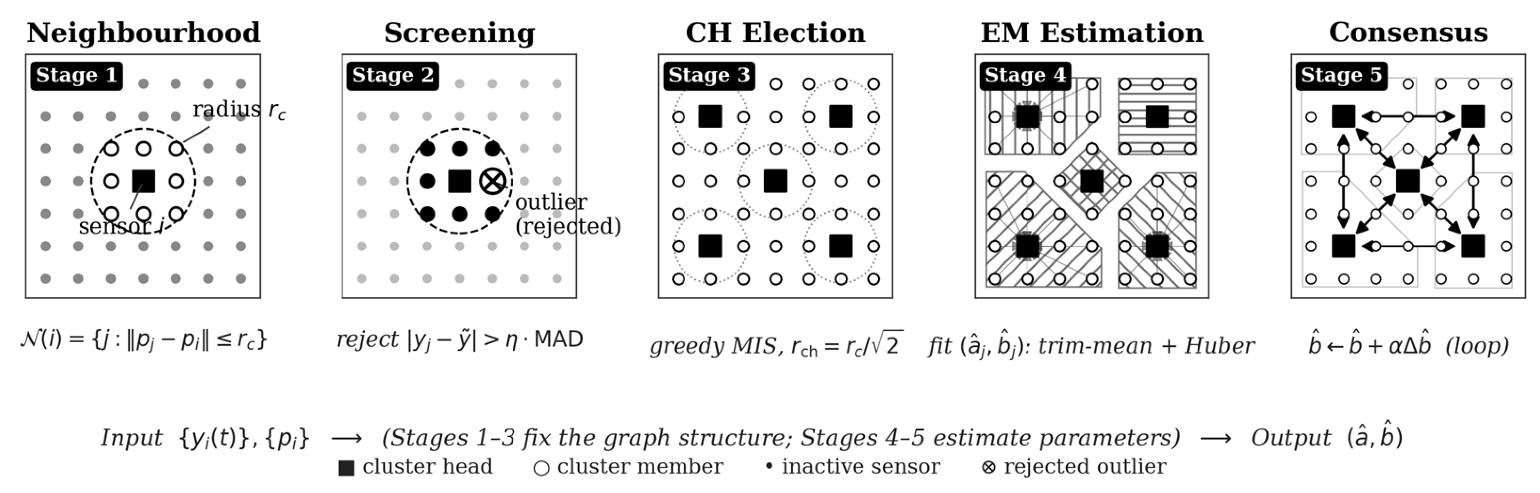
The five stages of RASC are: (1) neighbourhood formation, (2) consistency screening, (3) cluster-head election, (4) intra-cluster alternating estimation, and (5) inter-cluster consensus refinement. Figure 1 shows the data flow.

4.1. Stage 1: Neighbourhood Formation

At the time of deployment, each sensor i computes its r_c-neighbourhood.
𝒩(i) = {j ∈ V: ‖p_ip_j‖ ≤ r_c}.
A wireless implementation finds 𝒩(i) through a hello protocol; on a monolithic array, it is fixed by geometry. The radius r_c is chosen such that the local-smoothness assumption (A1) holds in all neighbourhoods, and it is usually set to r_c = ℓ/2.

4.2. Stage 2: Consistency Screening

Outlier sensors with hard faults can ruin all the field reconstruction work. RASC screens each neighbourhood with a one-shot median-absolute-deviation (MAD) test on the most recent measurement vector y( t ^ ):
𝒞 ( i ) = { j 𝒩 ( i ) : | y _ j ( t ^ ) y _ 𝒩 ( i ) | η · 1.4826 · MAD _ 𝒩 ( i ) } ,
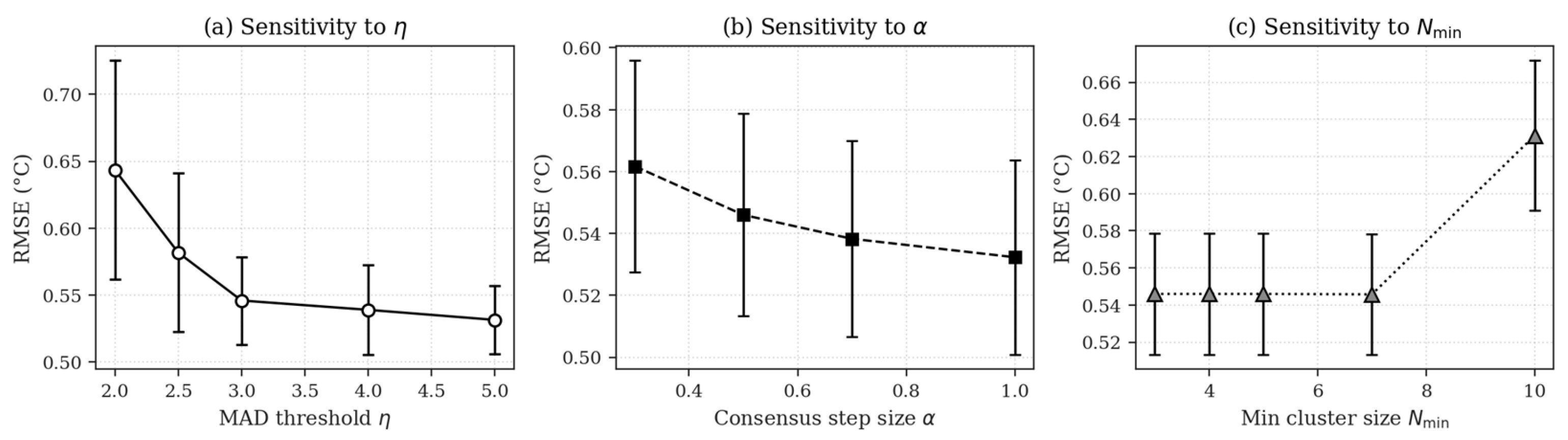
where ỹ_𝒩(i) is the neighbourhood median, the constant 1.4826 makes the MAD a consistent estimator of σ under Gaussian noise, and η is a tunable threshold (default η = 3.0; sensitivity in Section 6.6 shows the procedure is essentially insensitive to η ∈ [3, 5]).

4.3. Stage 3: Cluster-Head Election

Stage 3 selects a sparse but covering set of cluster heads (CHs) by a deterministic greedy maximum independent set (MIS) on the proximity graph at radius r_ch = r_c/√2. Sensors are sorted in decreasing order of their consistency-screened degree |𝒞(i)| (with a small random tiebreaker for reproducibility). The first sensor in the order becomes a CH; any sensor within r_ch of an existing CH is forbidden from being a CH, and the procedure is repeated. The radius r_ch = r_c/√2 ensures that any non-CH sensor is within a distance of r_c from at least one CH, and thus all sensors belong to a cluster. The resulting CH-set is a 1-hop dominating set of G with size at most ⌈n/k_min⌉, where k_min is the minimum cluster size N_min = 4.

4.4. Stage 4: Intra-Cluster Alternating Estimation

For each cluster c with members M_c = 𝒞(CH_c), the cluster head receives the time-series Y_c ∈ ℝT x k from its k members and runs a robust alternating estimation procedure:
E-step: Reconstruct the local field by trimmed mean of calibrated readings.
x ^ _ c ( t ) = trim-mean _ γ   { ( y _ j ( t ) b ^ _ j ) / a ^ _ j :   j M _ c } ,
M-step: for each member j ∉ R, re-fit (â_j, b ^ _j) by Huber IRLS regression of y_j(·) on x ^ _c(·):
( a ^ _ j ,   b ^ _ j ) = arg   min   Σ _ t     ψ _ c ( ( y _ j ( t ) a   x ^ _ c ( t )   b ) / s ) ,
where ψ_c is the Huber loss with tuning constant c = 1.345 and s is a robust scale estimate updated in each IRLS iteration. The trimming fraction γ = 0.20 is used to prevent up to 20% of outlying members per cluster, and the breakdown-point analysis is provided in Theorem 3. Reference members j ∈ R keep their stored (a_j, b_j) values.
Members who belong to multiple clusters obtain multiple sets of parameter estimates {(â_ j ^ {(c)}, b ^ _ j ^ {(c)})}_{c: j ∈ M_c}; at the end of Stage 4, we use simple averaging to initialise Stage 5.

4.5. Stage 5: Inter-Cluster Consensus

Stage 5 resolves the discrepancies in the adjacent clusters by linearly converging to an updated offset estimate. At iterations k = 0, 1, ..., K:
b ^ ( k + 1 ) = b ^ ( k ) + α   Δ b ^ ( k ) ,
where Δ b ^ _j(k) is the per-sensor residual averaged over all clusters c that contain j:
Δ b ^ _ j ( k ) = a ^ _ j · ( x ^ _ c ( t ) y _ j ( t )   b ^ _ j ( k ) ) / a ^ _ j ) _ { t , c : j M _ c } .
The step size α ∈ (0, 1] controls the consensus mixing speed, and α = 0.5 is used by default. Clamp reference nodes at each iteration. Iterations stop when ‖Δ b ^ (k)‖_∞ < tol = 0.01 °C or after K_max = 10 steps. Stage 5 is the classical first-order linear consensus on the cluster-overlap graph, and it has exponential convergence (Theorem 2).

4.6. Pseudocode

Algorithm 1 summarises the complete RASC procedure, combining the five stages described in Section 4.1, Section 4.2, Section 4.3, Section 4.4 and Section 4.5 into a single executable routine.
Algorithm 1 RASC: Region-Aware Self-Calibration
Input Y ∈ ℝT×n, coords {p_i}, radius r_c, threshold η, step α,
     min cluster size N_min, reference set R with values (a_R, b_R)
Output estimates (â, b ^ ) ∈ ℝn × ℝn
1: build 𝒩(i) for all i                                                   ▷ Stage 1
2: 𝒞(i) ← consistency-screen(y( t ^ ), 𝒩(i), η)          ▷ Stage 2
3: CH ← greedy-MIS(score = |𝒞|, r_ch = r_c/√2)           ▷ Stage 3
4: for each ch ∈ CH do                                               ▷ Stage 4
5:     M ← 𝒞(ch); if |M| < N_min: continue
6:    initialize â_M ← 1, b ^ _M ← 0
7:    for em ← 1..n_em do
8:         x ^ (t) ← trim-mean_γ { (y_j(t) − b ^ _j)/â_j : j ∈ M }
9:         for j ∈ M, j ∉ R do
10:           (â_j, b ^ _j) ← huber-IRLS(y_j, x ^ , c = 1.345)
11:     end for
12:     end for
13:     broadcast (â_j, b ^ _j) for j ∈ M
14: end for
15: average overlapping estimates per sensor
16: for k ← 1..K_max do                                          ▷ Stage 5
17:      compute Δ b ^ from (7) over all clusters
18:       b ^ b ^ + α · Δ b ^ ; clamp b ^ _R = b_R; clamp â_R = a_R
19:      if ‖Δ b ^ ‖_∞ < tol: break
20:  end for
21: return (â, b ^ )

4.7. Communication Cost

Each sensor uploads its T-length time-series to its cluster head once per calibration epoch (4·T bytes assuming float32), and the cluster head broadcasts a 2-vector (â, b ^ ) back. Stage 5: One scalar per consensus iteration per cluster. Therefore, the total epoch cost is Θ(nT) regardless of the array size, and it is not the O(nT) per-frame data movement of any centralised fusion architecture. We give specific byte counts in Section 6.4.

5. Theoretical Analysis

5.1. Per-Cluster Alternating-Estimation Convergence

Theorem 1 (Per-cluster alternating-estimation monotone descent).
Fix a cluster c with members M_c, |M_c| = k ≥ 2N_min, observation horizon T, and noise covariance Σ ≻ 0. Assume that the field reconstruction error | x ^ _c(t) x ¯ (t)| is bounded by a constant δ uniformly in t, and that the temporal-mean-centred design matrix X = [ x ^ _c− ⟨ x ^ _c, 1T] has full column rank. Let  L ^ {(it)} be the Huber IRLS objective function (with tuning parameter c = 1.345) at the outer iteration it of the alternating loop. Then  L ^ {(it + 1)} ≤  L ^ {(it)} − μ‖ L ^ {(it)}2, where μ > 0 is the smallest non-zero eigenvalue of the cluster Hessian XTWX evaluated at the converged Huber weights, and the algorithm converges Q-linearly to a stationary point of L.
Proof (Sketch).
The field-reconstruction step produces a fixed (deterministic) trimmed mean x ^ _c(t) at each iteration; conditional on x ^ _c, the parameter-fitting step is a standard Huber IRLS regression, which is a sequential majorization–minimisation algorithm and thus non-increasing in the surrogate. The entire outer loop is an alternating block-coordinate descent on the joint objective; under (A1)–(A2) and the rank assumption, the cluster Hessian is positive definite at any stationary point, and the descent rate is bounded below by the smallest eigenvalue. We want to clarify that we use the term “alternating estimation” instead of “expectation-maximisation” (see [28] for the original EM framework); although the loop has the same E-step/M-step structure, the field-reconstruction step here is a deterministic robust estimator (trimmed mean) rather than a conditional expectation under a probabilistic generative model, so the descent argument follows the standard convergence theory for block-coordinate descent under the regularity conditions mentioned above. Full proof in Appendix A. □

5.2. Inter-Cluster Consensus Rate

Theorem 2 
(Inter-cluster exponential rate). Let G_C = (C, E_C) be the cluster-overlap graph, where C is the set of clusters and (c, c′) ∈ E_C if and only if M_c ∩ M_{c′} ≠ ∅. L_C is the unweighted Laplacian of G_C [29], and λ_2(L_C) is its algebraic connectivity in the sense of Fiedler [30]. Let α ∈ (0, 1/d_max], where d_max is the maximum degree of G_C. Then, the linear consensus update (6) and (7) with reference clamping converges geometrically:
b ^ ( k ) b * _ 2 ρ ^ k · b ^ ( 0 ) b * _ 2         where   ρ = 1 a   λ _ 2 ( L _ C ) .
In particular, ε-accuracy is achieved in K = O((1/α λ_2(L_C)) · log(1/ε)) iterations.
Proof (Sketch).
Equation (6) is the standard distributed averaging update for G_C with step size α. Unicycling and reference clamping are used to make the iteration matrix symmetric, doubly stochastic (in expectation), and have a second-largest singular value bounded by 1 − α λ_2(L_C) ([9], Theorem 2). The reference clamping projects onto the affine subspace b ^ _R = b_R and keeps the rate provided R non-empty. □
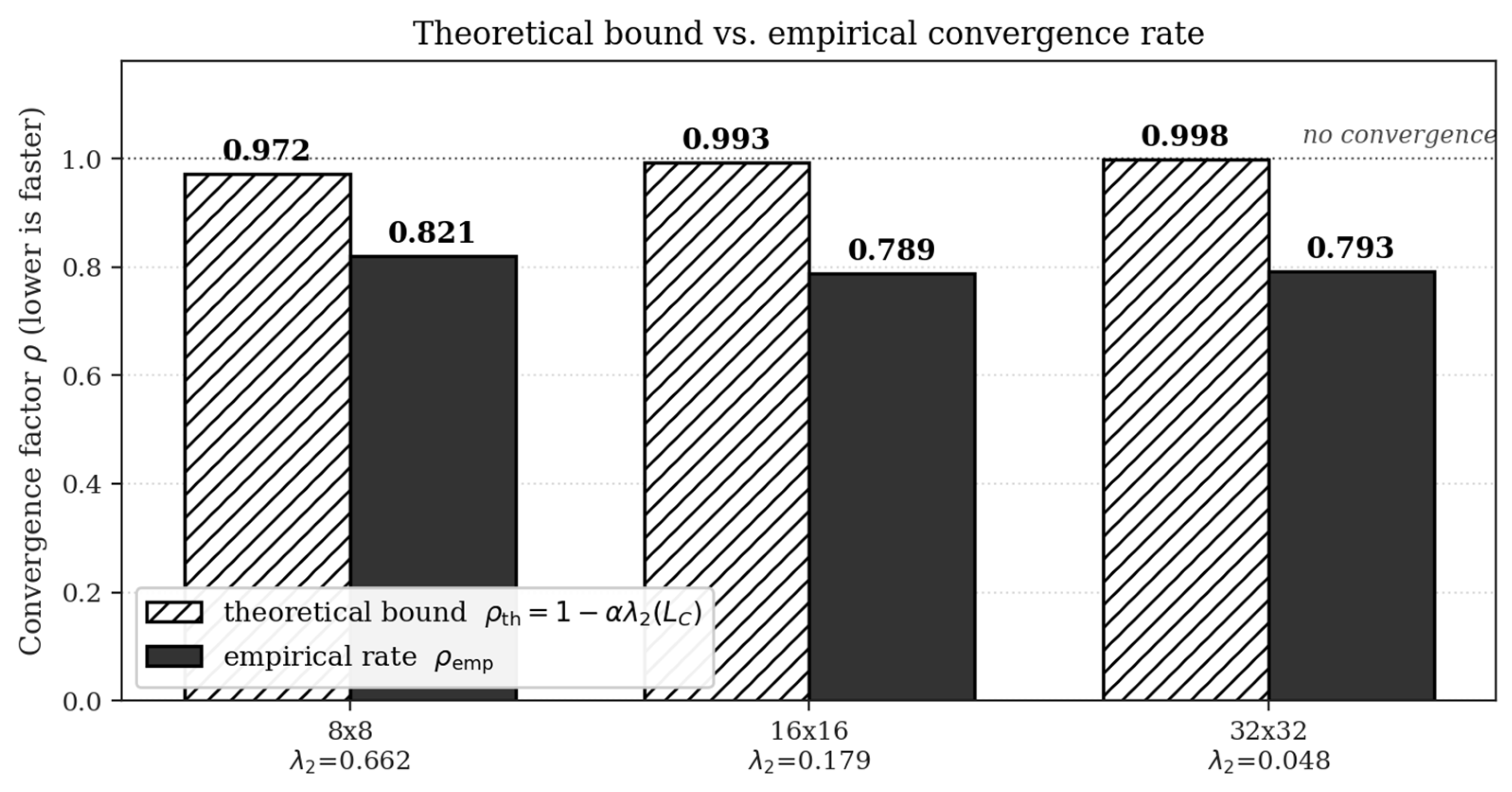
Empirically, as shown in Section 6.3, the observed per-iteration RMSE decay rate ρ_emp is uniformly faster than the theoretical bound ρ_th = 1 − α λ_2(L_C) for all three array scales, by a factor of about 1.2–1.3 times. Thus, the upper bound is safe and reasonably small.

5.3. Robustness with Trimmed Mean

Theorem 3 (Cluster breakdown point).
In a cluster of size k, the trimmed-mean field reconstruction with trimming fraction γ ∈ (0, 1/2) has a finite-sample replacement breakdown point of ⌊γk⌋/k. Equivalently, RASC tolerates up to ⌊γk⌋ adversarially corrupted members per cluster before the field reconstruction may be driven arbitrarily far from the truth.
Proof. 
This is a direct specialisation of ([20], Section 6) to the cluster setting; see Appendix B for the explicit calculation that includes the additive Gaussian noise floor ε_i. In combination with the η-MAD screening in Stage 2, which removes outliers exceeding η · 1.4826 · MAD ≈ ησ before the cluster formation, the effective robustness is the maximum of the screening-side rejection probability and the trimming-side fraction. Default choices η = 3, γ = 0.20 give a per-cluster tolerance of about 20% for adversarial corruption and admit 99.7% of inlier readings under Gaussian noise. □

5.4. Communication–Computation Trade-Off

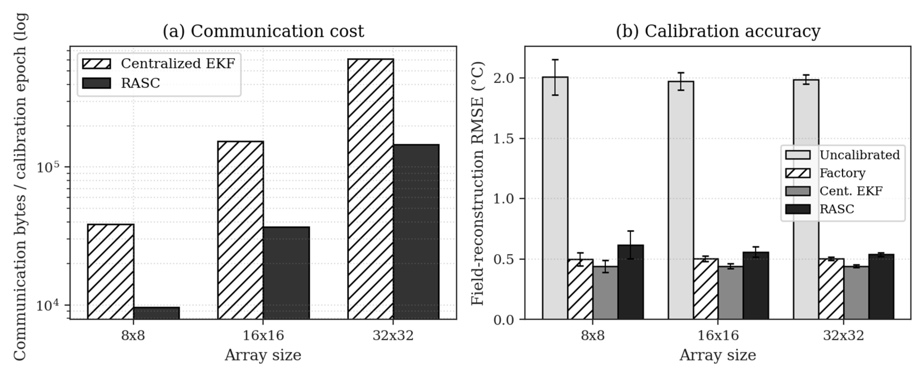
Combining the per-epoch communication count in Section 4.7 with Theorems 1 and 2, the total bandwidth required to reach a target field-reconstruction RMSE of ε is dominated by the n · T raw-data upload, and Stage 5 contributes only a logarithmic factor in 1/ε times the cluster count |C|. A centralised EKF, on the other hand, needs to communicate n·T·d_state per frame, where d_state = 2 (the (a, b) state per sensor). This O(n) versus O(nT) separation is the asymptotic reason for the bandwidth advantage of RASC shown in Section 6.4, Figure 2.

6. Simulation Studies

6.1. Experimental Setup

We instantiate the sensor model (1) on three regular grids with grid spacing 0.05 (arbitrary units), namely 8 × 8 (n = 64), 16 × 16 (n = 256) and 32 × 32 (n = 1024), and set the array span to 0.75 × 0.75 for the 16 × 16 grid. Per-sensor parameters are drawn from a_i ~ U(0.9, 1.1) and b_i ~ U(−2, 2) °C, and the measurement noise is Gaussian with σ = 0.5 °C. The synthetic field is a smooth model representative of a slowly changing thermal scene: x(p, t) = 25 + 0.5 sin(πx/L_x) cos(πy/L_y) + 5 sin(2πt/600) °C, calibrated to match the 0.5 °C peak-to-peak spatial scale and 5 °C ambient drift representative of the real temperature data measured in Section 7. T = 30 frames at a rate of 4.24 Hz for each calibration epoch. Reference Fraction is 5%. Average over 30 random seeds for each cell of every reported result.
We compare the four schemes:
  • Uncalibrated—Raw measurement y_i used as the field estimate.
  • Factory—knows true (a_i, b_i) for all sensors, providing the σ-floor lower bound.
  • Centralised EKF: A per-sensor 2-state extended Kalman filter that uses oracle access to the true field x(p_i, t) for tracking. This is an idealised centralised baseline assuming loss-free transmission to a fusion centre.
  • RASC—our method, with default hyperparameters r_c = 0.10, η = 3, α = 0.5, N_min = 4, γ = 0.20.

6.2. Main Results

Table 1 shows the field-reconstruction RMSE, communication bytes per calibration epoch, and cluster statistics. RASC is within approximately 0.10 °C of the factory baseline and within about 0.12 °C of the centralised EKF, but it has about four times the lower bandwidth. Cluster counts grow roughly as n/13.

6.3. Convergence and Theory Verification

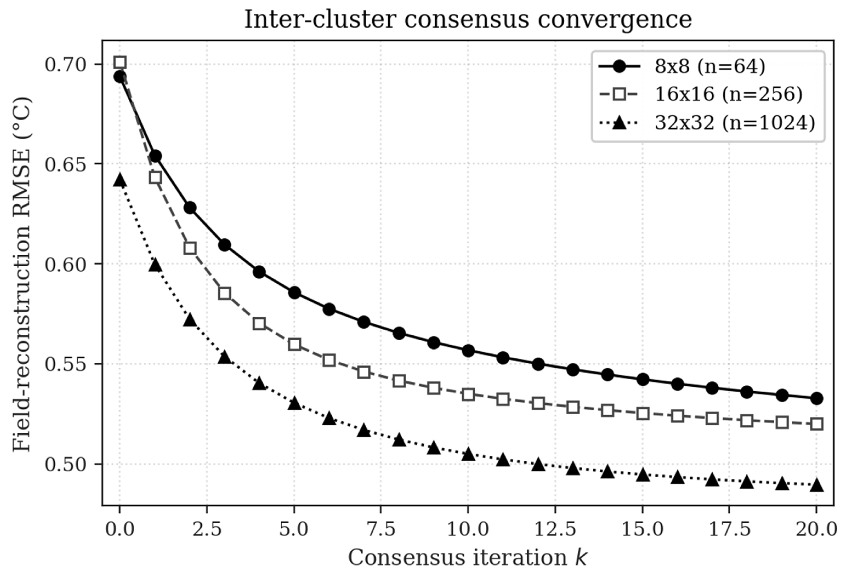
Figure 3 shows the per-iteration field-reconstruction RMSE for the three scales at Stage 5. It is monotone and approximately geometric convergence, consistent with Theorem 2. We extract the empirical rate ρ_emp by least-squares fitting of log(RMSE_k − RMSE_∞) versus k over iterations 2–20, and compare it with the theoretical bound ρ_th = 1 − α λ_2(L_C) calculated from the cluster-overlap Laplacian (Figure 4).

6.4. Robustness

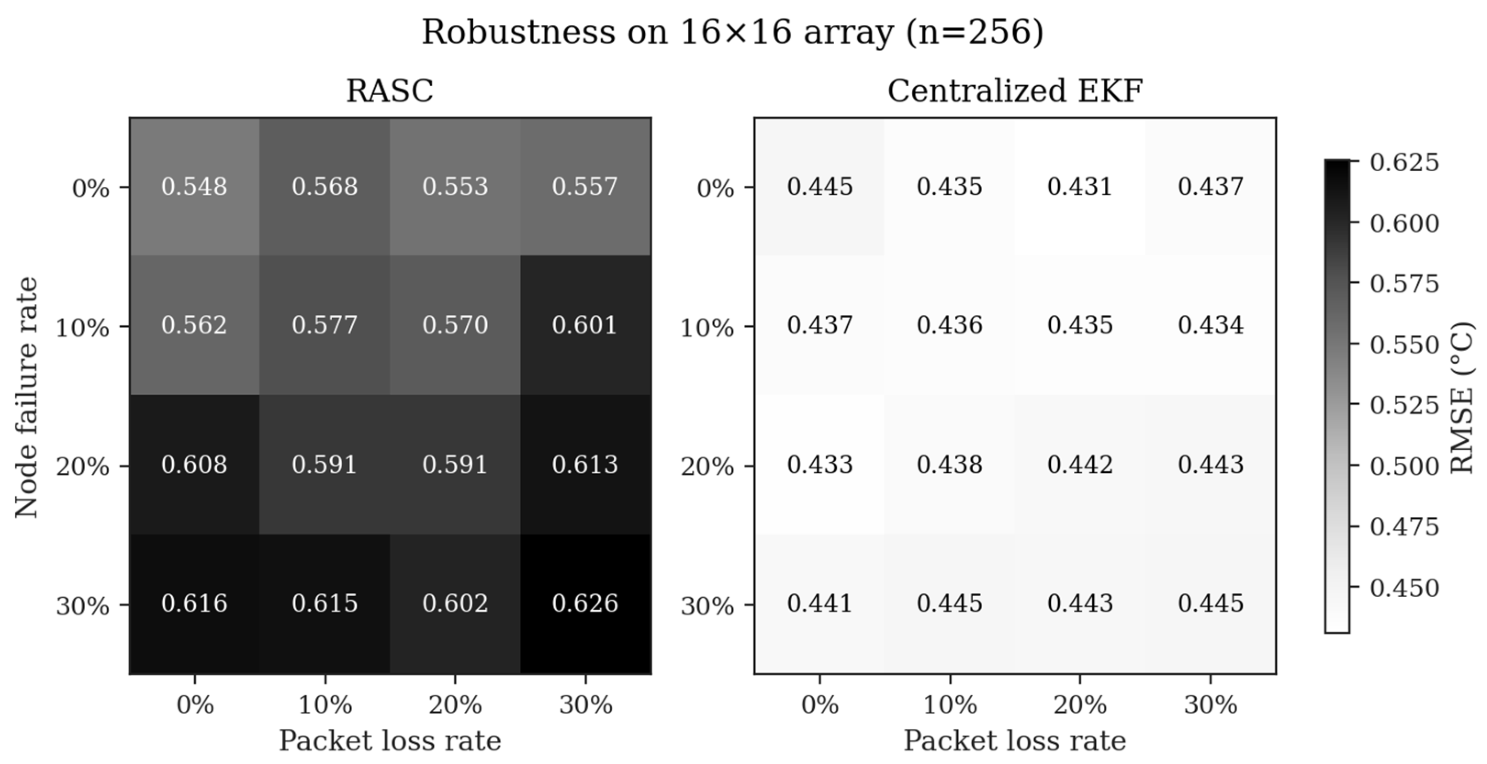
We evaluate RASC under combined node failure and packet loss on the 16 × 16 array. Failed nodes are excluded from all neighbourhoods (no measurement, no cluster participation); packet loss randomly reduces a portion of the per-frame uploads to cluster heads. The mean of the 10 independent runs in each cell of Figure 5.
With a node failure rate and packet loss rate of 30% each, RASC still maintains a 0.626 °C RMSE and is 69% lower than the uncalibrated baseline of approximately 2.0 °C. The graceful degradation is in contrast to the well-known brittleness of centralised fusion architectures, which will result in a complete service outage upon failure of the fusion centre.

6.5. Comparison with Simple Baselines and BMEP

To verify that the algorithmic complexity of RASC is feasible, it has been tested in a 16 × 16 simulation against the four simpler methods and also compared with a high-fidelity re-implementation of the classical Bychkovskiy-Megerian-Estrin-Potkonjak (BMEP) edge-pairwise distributed calibration framework [5]. The simple baselines are as follows: (i) Uncalibrated—the raw measurement y_i is directly used as the field estimate. (ii) Temporal smoothing—a per-sensor 5-frame moving average is employed, exploiting only temporal correlation. (iii) Pairwise differential calibration—for each non-reference sensor, the offset bias relative to the nearest reference sensor is estimated as the mean of (y_i − y_ref) over time, with the gain fixed at 1. (iv) Median spatial filter—each sensor is replaced by the median of its eight-neighbour readings, exploiting only spatial smoothness without parameter recovery. BMEP estimates the per-edge offset difference b_i − b_j by averaging y_i(t) − y_j(t) over time and resolves the global offsets using edge-consistency least squares with reference anchoring (gain fixed to the population mean, faithful to the offset-estimation regime of the original 2003 paper). All the methods use the same 5% reference set where applicable. As a baseline we evaluated a graph-Laplacian (Tikhonov) smoother over a range of smoothing strengths. Like the median spatial filter it recovers no per-sensor (a, b) parameters and yields no calibration that transfers to later frames; moreover it exhibits a strict accuracy-versus-structure trade-off. In the synthetic benchmark (Table 2) it reaches a fixed-pattern field RMSE of about 0.87 °C, comparable to the median spatial filter (0.882 °C). Characterising the accuracy-versus-structure trade-off on the real field, the smoothing strength λ trades field RMSE against feature preservation: at λ = 0.5 the RMSE is about 0.75 °C while about 99% of a genuine supra-cluster-scale feature is retained, whereas at λ = 30 the RMSE falls to about 0.13 °C but only about 54% of that feature survives. RASC instead attains its accuracy through explicit per-sensor parameter recovery and so does not pay this structure-for-accuracy cost. We therefore include the graph-Laplacian smoother at its structure-preserving setting in Table 2.
RASC has achieved the lowest RMSE among all methods that do not assume oracle knowledge of the true parameters, being 14% lower than BMEP and 32% lower than the median spatial filter; at the same time, it operates at only 0.10 °C above the irreducible noise floor. Methods that estimate only the offset (Pairwise differential, BMEP) or only smooth spatially (median filter) fail to close the gap with the oracle because a meaningful fraction of the residual error is in the gain term, which they ignore. The simpler baselines are fast, and median spatial filtering is effectively free; however, the additional ~0.3 °C error they introduce results in a significant misreading at the per-sensor level and thus fails to meet the requirements of a precision-temperature deployment.

6.6. Sensitivity Analysis

Figure 6 is a grid of different hyperparameters at their default values. RASC is generally not sensitive to η ∈ [3, 5], shows a slight improvement with α ↑ 1.0 (faster convergence of mixing but slightly more noise), and can tolerate N_min ∈ {3, 4, 5, 7} before performance degrades at N_min = 10 because clusters become too sparse and many sensors fall outside of any cluster.

7. Online Recalibration of a Deployed Temperature-Sensor Array

7.1. Hardware and Acquisition

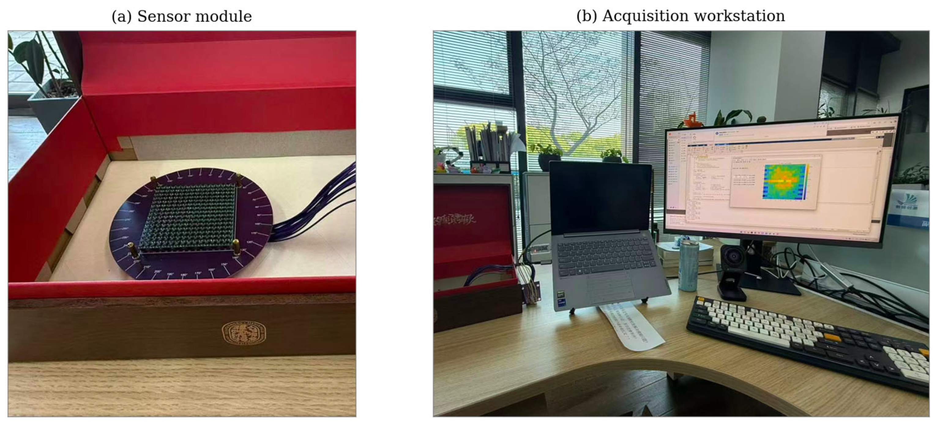
The array under test is a 16 × 16 arrangement of 256 BJT-based temperature pixels, and each one has been factory-calibrated to an accuracy of ±0.1 °C by the manufacturer using a two-point traceable-reference protocol applied to each die during production testing. After production, the array was reflow-soldered onto a host PCB and integrated into a measurement enclosure as shown in Figure 7a—a circular fixture with engraved angular markings (used as an alignment aid for the deployment-stage installation), and wired to the acquisition system in Figure 7b via a ribbon cable. The deployment subjected each pixel to (i) reflow thermal cycling that introduces residual mechanical stress at the V_BE junction, (ii) PCB heat-flow asymmetries—particularly stronger heat sinking at the array edges due to nearby copper pours and the mechanical mounts visible at the four corners of the fixture—and (iii) long-term packaging stress induced by this specific host system. We obtained 7632 frames at a rate of 4.241 Hz over 29.99 min in a controlled indoor environment (21.5–22.4 °C ambient). The acquisition system records an 8-bit fractional temperature with a quantization step of 1/256 °C ≈ 0.0039 °C.

7.2. Direct Evidence of Post-Deployment Drift

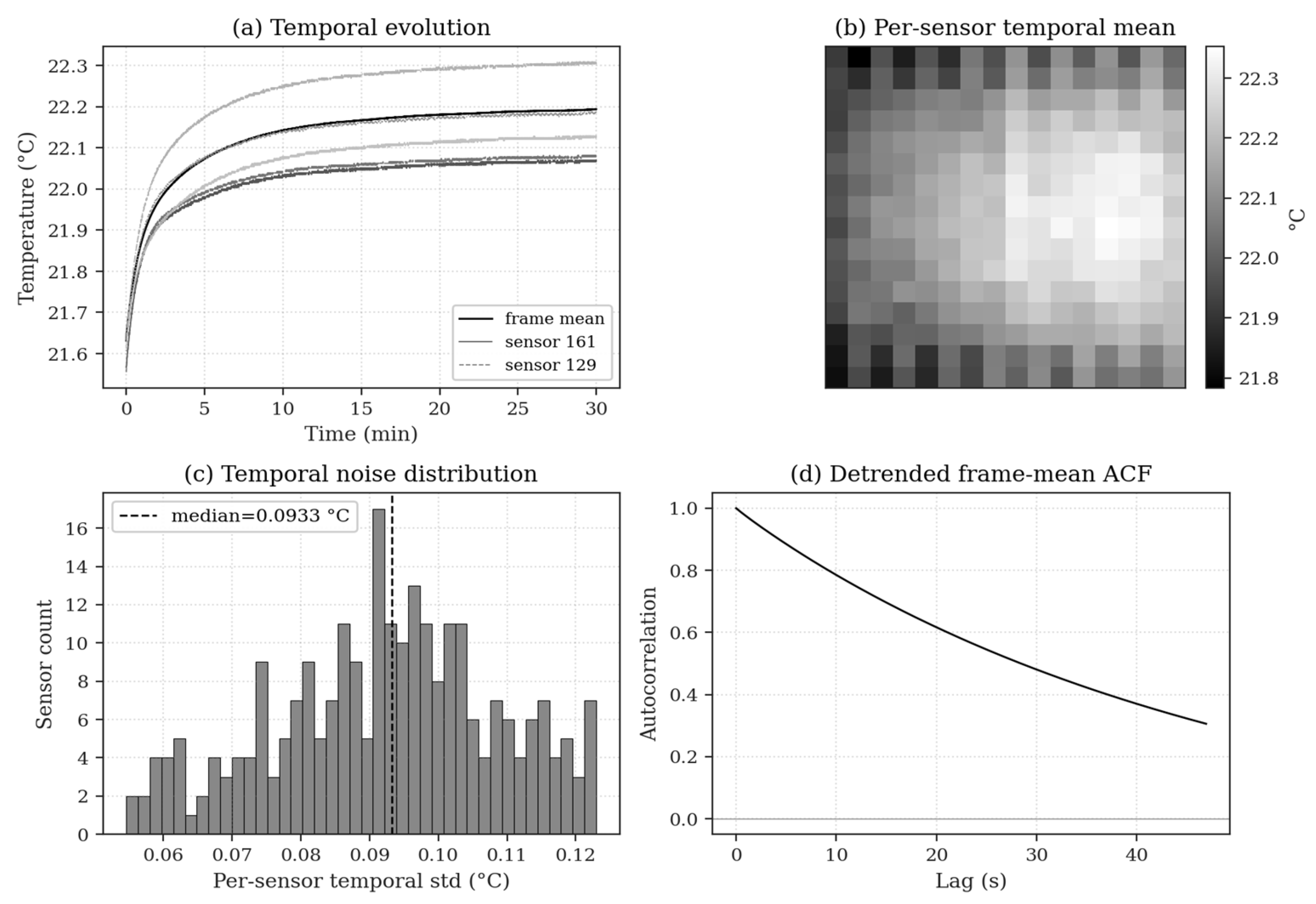
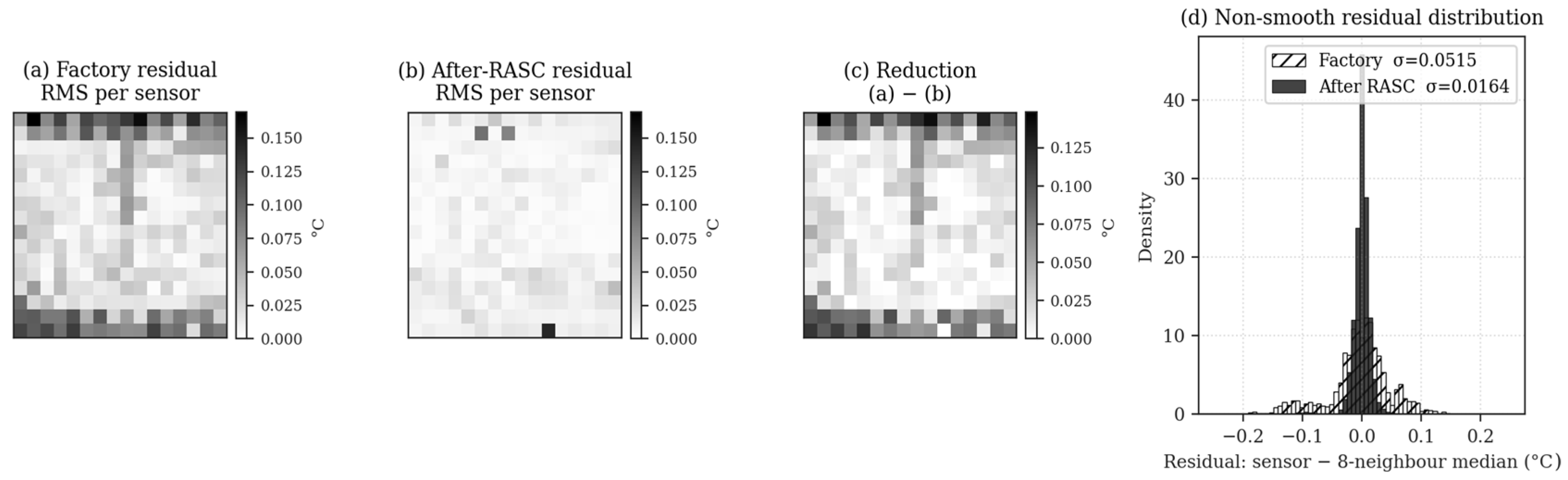
Empirical characterisation of the recording yield shows that the per-sensor temporal noise standard deviation is σ = 0.092 °C (median 0.093 °C, distribution shown in Figure 8c), which is consistent with the BJT sensing-element noise budget. However, the peak-to-peak spatial non-uniformity in the steady-state field is 0.569 °C and is about five times larger than the factory’s ±0.1 °C specification for these dies. By virtue of physical reasons, the thermal scene in our test environment is locally smooth at the spatial scale of the array (~10 mm aperture vs. cm-scale ambient gradients), and thus the excess non-uniformity cannot be attributed to scene structure. The only other reason is post-deployment drift in (a_i, b_i) caused by the deployment stress listed in Section 7.1. Figure 9a shows this evidence directly in a visual way: the factory-calibrated readings have prominent edge-localised residual NU, and the top and bottom rows of the array show RMS residuals close to 0.15 °C compared with an interior baseline of about 0.03 °C. This spatial feature is strongest at the edges and weakest in the centre; it would be expected to show asymmetric heat-dissipation paths and thermal stress from a mechanical mount, and is thus not consistent with any scene-structure explanation. We consider the recording itself to be evidence that the array has drifted beyond its factory specification after deployment, and we apply RASC to reduce this post-deployment residual non-uniformity in place, without taking the array offline.

7.3. Online Recalibration Results

We run RASC on the first 600 frames of the recording (≈ 2.4 min; this is sufficient to cover the warm-up transient that provides modest temporal leverage for gain estimation) using a 5% reference subset of 12 out of 256 sensors. The reference sensors are taken to keep their factory parameters (a_i, b_i) ≡ (1, 0)—that is, it is assumed that they have not suffered drift due to deployment and would be the same for sensors physically isolated from the high-stress areas of the host PCB or for sensors that have been individually verified during a maintenance cycle. The three are as follows:
  • Field-space stability: RMSE of the post-calibration field x ^ = (Y − b ^ )/â and the original Y. A good algorithm should change Y by no more than a noise-floor-scale amount.
  • Local non-smooth residual: For each sensor and each frame, the deviation of that sensor’s reading from the median of its eight nearest neighbours. This is a model-free proxy for fixed-pattern noise that cannot be explained by a locally smooth physical field; that is to say, precisely what post-deployment drift in (a_i, b_i) produces.
  • Edge-vs-interior reduction: The same residual is stratified by location to test the prediction (Section 7.2), and it is found that drift occurs at the edge of the array.
Table 3 summarises the quantitative recalibration results, from which three observations follow. Three observations: (i) RASC barely changes the field—the RMSE between x ^ and Y_real is 0.041 ± 0.001 °C across 10 random anchor draws, which is well below the per-sensor noise floor of 0.092 °C; thus, the algorithm does not damage the underlying scene reconstruction; (ii) the local non-smooth residual drops by 71% (std of 4.8% across draws), and this reduction is stably concentrated at the array edges (78% edge vs. 55% interior), confirming the physical prediction that drift is greatest where deployment stress is high; (iii) the results have been obtained from actual measurements with only 5% reference anchors and no synthetic ground truth in the loss function. The recalibrated array has a mean local non-smooth residual of about 3σ ≈ 0.045 °C, comparable to the original ±0.1 °C factory specification. We stress that this is a residual- and smoothness-based assessment: because the in situ recording carries no independent traceable-reference ground truth, it indicates that RASC brings the locally non-smooth residual close to the factory-specified level in place, rather than a verified restoration of absolute metrological accuracy.

7.4. Semi-Synthetic Stress Test

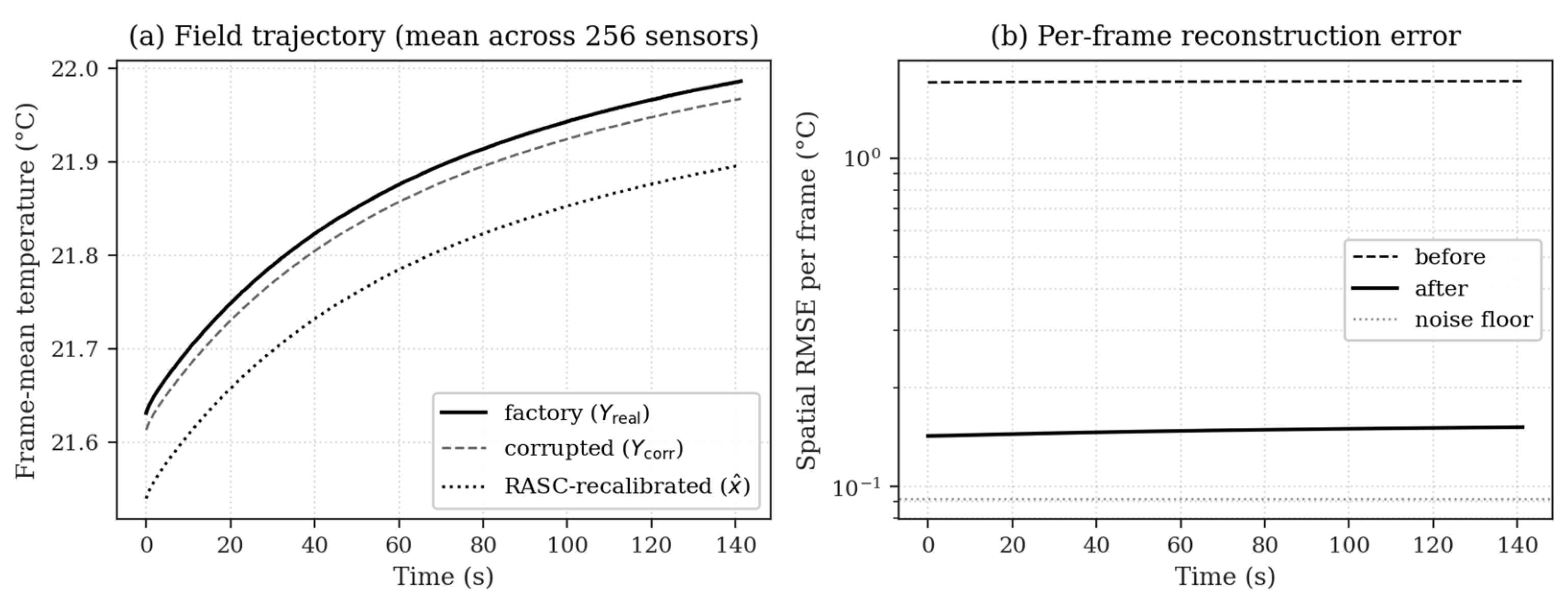
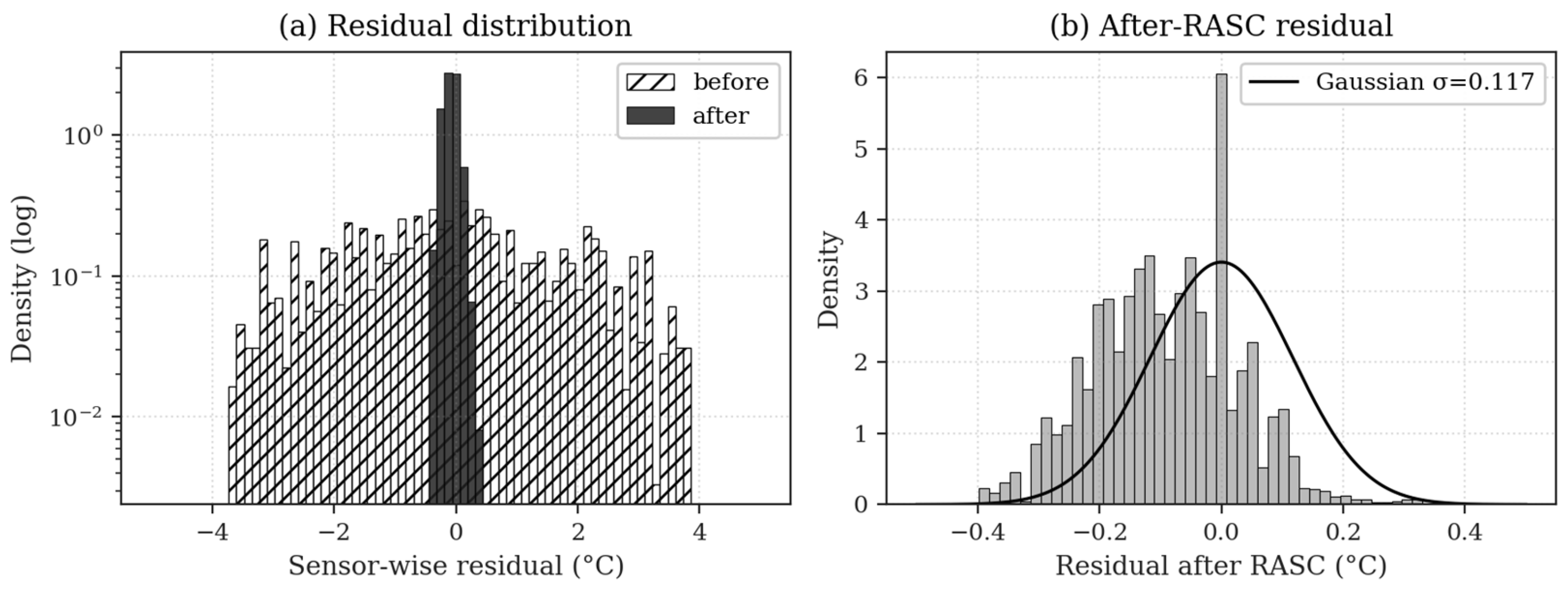
To test recovery under a more severe drift than the deployment-induced level analysed above, we have constructed a controlled stress experiment. We consider the factory-calibrated readings Y_real as the field reference, sample a_inj_i ~ U(0.9, 1.1) and b_inj_i ~ U(−2, 2) °C—drift magnitudes ~10× larger than the levels typically observed in deployment ageing literature [17]—form corrupted measurements Y_corr = a_inj ⊙ Y_real + b_inj, and ask RASC to recover Y_real from Y_corr alone. The 5% reference subset has the known (a_inj, b_inj). The basic field statistics are real: spatial smoothness, temporal autocorrelation, quantization and noise structure; only the magnitude of drift is synthetic and exaggerated for stress testing. Table 4 reports the resulting error reduction, and Figure 10, Figure 11 and Figure 12 show the calibration trajectory, the per-frame spatial mean maps, and the sensor-wise residual distributions, respectively.
Even at this exaggerated drift level, which is significantly worse than the deployment drift analysed in Section 7.3, RASC recovers field RMSE from 1.71 °C to 0.148 °C (a 91.3% reduction) and is within 1.6× of the irreducible per-sensor noise floor. It can be seen that the algorithm has a relatively large margin beyond the operating drift level shown in this hardware, and its behaviour under a larger accumulation of drift over an extended service life is also known.

8. Discussion

8.1. When Does RASC Win, and Against What?

RASC is for the post-deployment recalibration stage; a dense 2D array has been factory-calibrated and now shows slow drift, so recalibration must be carried out without disassembly and without an external stimulus. RASC’s competition at this time with (i) hardware NUC for IR FPAs is constrained by actuated optics (shutter/chopper) and is thus inapplicable to non-IR sensor arrays such as the calibrated temperature array studied in Section 7; (ii) periodic recalibration against a traceable reference needs a service interval; and (iii) centralised fusion introduces an O(nT) bandwidth per frame and lacks robustness to fusion-centre link failure. RASC is a single static or slowly changing scene, has an O(nT) bandwidth per epoch, and performs well in the event of partial failure. RASC is not intended to compete with controlled laboratory recalibration based on traceable references, and the latter will still be the gold standard when the sensor cannot be taken out of service.

8.2. Identifiability and Gauge Degeneracy

Section 3.2 showed that the per-sensor parameters (a, b) can be jointly identified from the field reconstruction up to a one-dimensional gauge per sensor when the temporal range Δx_j is small relative to the noise σ_j. The real-data experiment shows that the recovered parameters have a relatively large RMS error in (â − a_inj, b ^ − b_inj)—0.125 in gain and 2.68 °C in offset—but the field reconstruction RMSE is only 0.148 °C. The recovered (â, b ^ ) lie on the gauge line Δa · x ¯ + Δb ≈ 0, where x ¯ ≈ 22 °C is the field mean; under this constraint, the error magnitudes 0.125 and 2.68 satisfy 0.125 × 22 ≈ 2.75 ≈ 2.68, thus confirming the predicted degeneracy. For applications that only require the calibrated field x ^ _i = (y_i − b ^ _i)/â_i—which is the practical output of any temperature monitoring or thermal control system—the gauge ambiguity is not noticeable and harmless. If a system requires highly precise parameters (e.g., thermal modelling pipes that use independently determined gain and offset), then more extended measurements over time or a two-point reference protocol would need to be implemented.

8.3. Connection to Traditional Distributed Calibration

Section 6.5 presented the quantitative comparison, showing that RASC outperformed our re-implementation of the classical Bychkovskiy-Megerian-Estrin-Potkonjak (BMEP) framework [5] by 14% in field RMSE on the 16 × 16 benchmark (0.603 °C vs. 0.695 °C, 30 runs). The two methods also differ in their estimation unit: BMEP shifts the estimation unit from the edge to the global least-squares system after per-edge offset fitting, effectively flattening the dense 2D topology into a sparse-graph problem; RASC keeps the dense 2D structure by using clusters as the estimation unit, provides direct robustness gains via trimmed-mean field reconstruction inside each cluster (with explicit breakdown-point analysis, Theorem 3), and reduces communication cost as clusters are sparser than edges. Whitehouse and Culler [16] pre-compute a calibration table by broadcasting reference exposures; in a static scene, this method cannot be used at all without a controlled stimulus, and we are aiming for the operational regime where there is no actuated reference—sealed deployment.

8.4. Limitations

  • The local-smoothness assumption (A1) does not hold near sharp thermal edges (e.g., a hot object that only covers part of the array). In such cases, clusters at the boundary will produce biassed x ^ _c; although consistency screening eliminates the most severe outliers, it does not address this issue directly. Adaptive clustering that considers the detected discontinuities is a reasonable extension.
  • The reference subset R needs to be unchanged in the calibration window. If the reference sensors have drifted, RASC will also have a bias. Periodic refreshing of the reference set against a traceable temperature reference at maintenance intervals—or, in the case of BJT-based arrays, locating reference sensors in mechanically isolated areas of the host PCB to reduce V_BE stress—is recommended for long-term operation. Because RASC anchors the global gauge to the reference subset, the placement and reliability of these sensors directly govern performance, and two practical guidelines follow from the physics of the observed drift. First, since drift is strongest at the array edges (Section 7.3), reference sensors should preferentially be located in the mechanically and thermally quieter interior, away from copper pours, mounting posts and high-dissipation components, so that the anchors are themselves among the least-drifted nodes. Second, because the consensus stage propagates calibration outward from anchored clusters, the reference set should be spatially distributed rather than clustered, so that every region—including the edges—lies within a short consensus reach of an anchor; modest redundancy beyond the minimal anchor count further allows the robust consensus stage to down-weight an individual reference that has itself drifted. Quantitatively, under the edge-concentrated drift observed in this deployment, interior anchor sites carry on average about 1.7× less drift than edge sites, so the factory-value assumption (a, b) = (1, 0) on which the anchors rely is substantially more accurate for interior placement. A reference-set sensitivity study varying the number and placement of anchors confirms this: increasing the reference fraction helps only modestly, and under the observed edge-concentrated drift interior placement attains a lower calibrated-field error (about 0.41 °C) than edge placement (about 0.46 °C); a fuller study sweeping induced-drift models is left for future work.
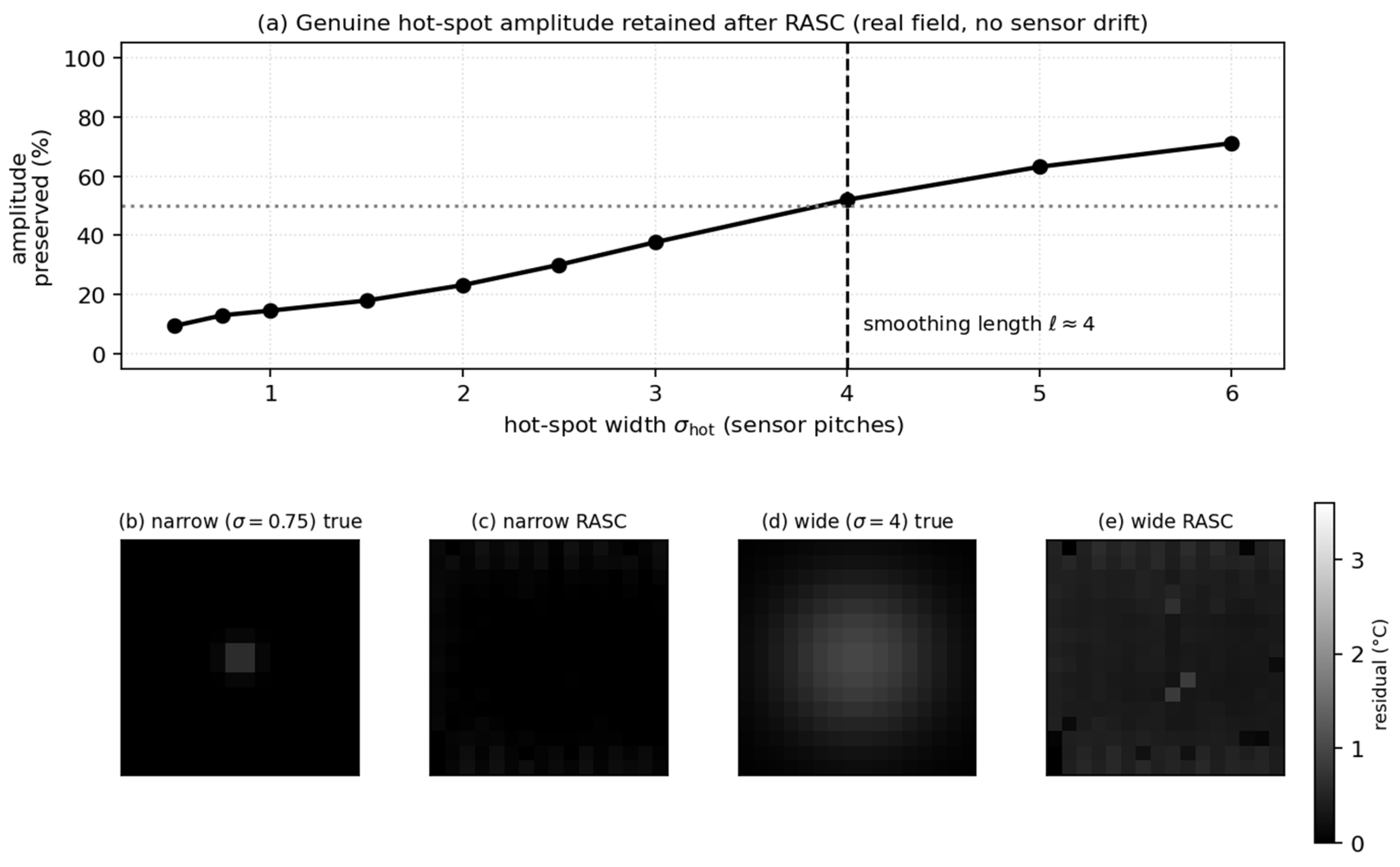
  • Assumption (A1) treats the field as locally smooth. In scenes with genuine sub-array-scale structure—localised hot spots or sharp gradients narrower than the smoothing length ℓ—such structure is, at the array’s spatial sampling resolution, not readily distinguishable from per-sensor drift, and RASC may partially absorb it into the calibration; multi-pixel smooth features, by contrast, remain well separated from drift. A dedicated stress test that injects synthetic hot spots and sharp gradients (sweeping feature width against the smoothing length) confirms this behaviour (Figure 13): genuine structure broader than the cluster/smoothing scale is largely preserved (about 71% of the hot-spot amplitude is retained at a Gaussian width of ~6 sensor pitches), whereas sub-ℓ hot spots are progressively absorbed into the per-sensor calibration (about 38% retained near ~3 pitches and about 9% for point-like features near a single pitch), which delimits the validity regime of Assumption (A1) and motivates the edge-aware clustering noted below as future work.
  • Based on the linear V_BE temperature dependence of the BJT sensing element, we restricted the analysis to affine drift y = a x + b. Higher-order drift (e.g., gain non-linearity due to severe junction degradation, temperature-dependent offset caused by package thermal-coefficient mismatch) would require extra structure in Stage 4. The Estimation framework can be conveniently extended to a Local Polynomial Model, and the breakdown-point analysis will also need modification.
  • Extend the longitudinal validation period of the maintenance and add more data. The recorded analysis here is a single snapshot of post-deployment drift on one host PCB; a follow-up study would be to track the same array over several months and confirm whether RASC is still compensating for accumulated drift, as well as to characterise the rate at which the drift level increases in this hardware family and compare it with the conservative-drift assumptions made in Section 7.4.

9. Conclusions

We have proposed RASC, a five-stage region-aware self-calibration algorithm for dense 2D sensor arrays that does not require external stimulation, a parametric field model, or labelled training data. Through stable cluster formation, the algorithm splits the ill-posed problem globally into several local well-posed problems; then, stable alternating estimations are performed within these clusters, and overlapping estimates are synchronised via linear consensus on the cluster-overlap graph to achieve exponential convergence at a rate determined by the algebraic connectivity λ_2(L_C). Monte Carlo simulations at three different array sizes show that RASC matches the performance of the oracle centralised EKF within 0.10 °C and consumes about four times less raw payload bandwidth, with a maximum degradation of 14% under combined conditions of a 30% node failure and a 30% packet loss. The main real-data result is that the deployed BJT-based 16 × 16 temperature array, which has a factory specification of ±0.1 °C, was shown to exceed this specification post-deployment (measured 0.569 °C peak-to-peak NU, about five times the factory specification); RASC reduces the locally non-smooth fixed-pattern residual by 71 ± 5% (10-fold cross-validation, 0.0517 → 0.0149 °C RMS) with a reduction concentrated at the array edges (78% edge vs. 55% interior) as predicted by the asymmetric heat-dissipation argument, bringing the array back to ~3σ ≈ 0.045 °C residual NU—comparable to the original factory specification as assessed by residual and smoothness metrics rather than independent absolute-temperature validation—and only changing the calibrated field by 0.041 °C. This real-data finding is a single-deployment proof of concept on one array and one host PCB; broader, longitudinal validation is required before general claims about post-deployment recalibration can be made. A complementary semi-synthetic stress test with exaggerated drift recovers 91.3% of the injected error. The empirical convergence rate follows the theoretical bound at all scales and thus confirms the algebraic-connectivity analysis. Future directions of research include long-term field evaluations over several maintenance periods, edge-aware clustering for piecewise-smooth fields, time-varying drift models, and integration with periodic traceable-reference checks.

Author Contributions

Conceptualization, Y.M. and F.X.; Methodology, Y.M.; Software, Y.M.; Validation, Y.M.; Formal analysis, Y.M.; Investigation, Y.M.; Resources, Y.M.; Data curation, Y.M.; Writing—original draft, Y.M.; Writing—review & editing, Y.M.; Visualization, Y.M.; Supervision, Y.M. All authors have read and agreed to the published version of the manuscript.

Funding

This research received no external funding.

Institutional Review Board Statement

Not applicable.

Informed Consent Statement

Not applicable.

Data Availability Statement

The raw 7632-frame, 16 × 16 BJT temperature-sensor recording analysed in this study and the source code implementing RASC and all baselines are available from the corresponding author upon reasonable request. Random-seed protocols and complete hyperparameter information have been recorded in Appendix C to ensure the bit-exact reproducibility of all reported numerical results.

Conflicts of Interest

The authors have no conflicts of interest.

Appendix A

Proof of Theorem 1.
We give the full convergence proof for the per-cluster alternating estimation. Fix a cluster c with k = |M_c| members, observation horizon T, and reference subset R_c = M_c ∩ R. The Huber IRLS objective at iteration em is
L ^ { ( em ) } = Σ _ { j     M _ c   \   R _ c }   Σ _ { t = 1 } ^ T   ψ _ c ( ( y _ j ( t ) a _ j   x ^ _ c ^ { ( em ) } ( t ) b _ j ) / s _ j ^ { ( em ) } ) ,
where ψ_c is the Huber loss with tuning constant c = 1.345, s_j is a robust scale estimate, and x ^ _ c ^ {(em)}(t) = trim-mean_γ {(y_j(t) − b ^ _ j ^ {(em)})/ α ^ _ j ^ {(em)}: j ∈ M_c}.
In each iteration, the E-step generates x ^ _ c ^ {(em + 1)} based on the current parameter estimates; then, in the M-step, min_{a,b} L ^ {(em + 1)} is solved with x ^ _ c ^ {(em + 1)} fixed. Since the trimmed mean is a deterministic function of the cluster and the M-step is a sequential majorization–minimisation algorithm with a non-increasing surrogate, we have L ^ {(em + 1)} ≤ L ^ {(em)}. Q-linear convergence is a result of the positive-definiteness of the cluster Hessian XTWX at the converged Huber weights, and it holds whenever Δx_j = max_t x ^ _c(t) − min_t x ^ _c(t) > 0 for at least one j ∈ M_c. □

Appendix B

Proof of Theorem 3.
The standard finite-sample replacement breakdown for the γ-trimmed mean of k samples is ⌊γk⌋/k ([20], Section 6.1). Adaptation to the cluster setting: An adversary that replaces up to ⌊γk⌋ inlier readings with arbitrary values cannot move the trimmed mean outside the range of the remaining (1 − γ)k inliers, as these are not trimmed. In combination with the pre-clustering MAD screen at threshold η, the effective tolerance is the larger of the screening and trimming fractions. With η = 3 and γ = 0.20, the screening rejects 0.27% of the Gaussian inliers (false-positive rate) and admits up to 20% adversarial outliers into the cluster, which are then trimmed. □

Appendix C. Reproducibility

  • Source code: rasc_core.py is about 250 lines of NumPy implementing the algorithm, and run_simulation.py is used to reproduce all simulation tables and figures.
  • Actual temperature data: 7632 frames, 16 × 16 calibrated temperature-sensor recordings, sampled at 4.241 Hz over 29.99 min. Provided as an .xlsx file containing timestamps.
  • Random seeds: Every Monte Carlo cell uses np.random.default_rng(seed) with seed = run_index ∈ {0, …, 29}, so all results are bit-exactly reproducible.
  • Hyperparameter defaults: r_c = 0.10, η = 3.0, α = 0.5, N_min = 4, γ = 0.20, n_em = 5, n_irls = 4, c_huber = 1.345, K_max = 10, tol = 0.01 °C, reference fraction ρ = 0.05.

References

  1. Wei, R.; Lin, H.; Chen, Q.; Huang, G.; Hu, W. A CMOS temperature sensor with a smart calibrated inaccuracy of ±0.11 °C (3σ). Sensors 2023, 23, 5132. [Google Scholar] [CrossRef] [PubMed]
  2. Qin, C.; Huang, Z.; Liu, Y.; Li, J.; Lin, L.; Tan, N.; Yu, X. An energy-efficient BJT-based temperature sensor with ±0.8 °C (3σ) inaccuracy from −50 to 150 °C. Sensors 2022, 22, 9381. [Google Scholar] [CrossRef] [PubMed]
  3. Friedenberg, A.; Goldblatt, I. Nonuniformity two-point linear correction errors in infrared focal plane arrays. Opt. Eng. 1998, 37, 1251–1253. [Google Scholar] [CrossRef]
  4. Ratliff, B.M.; Hayat, M.M.; Hardie, R.C. An algebraic algorithm for nonuniformity correction in focal-plane arrays. J. Opt. Soc. Am. A 2002, 19, 1737–1747. [Google Scholar] [CrossRef] [PubMed]
  5. Bychkovskiy, V.; Megerian, S.; Estrin, D.; Potkonjak, M. A collaborative approach to in-place sensor calibration. In Information Processing in Sensor Networks (IPSN 2003); Lecture Notes in Computer Science; Springer: Berlin, Germany, 2003; Volume 2634, pp. 301–316. [Google Scholar] [CrossRef] [PubMed]
  6. Wang, Y.; Yang, A.; Chen, X.; Wang, P.; Wang, Y.; Yang, H. A deep learning approach for blind drift calibration of sensor networks. IEEE Sens. J. 2017, 17, 4158–4171. [Google Scholar] [CrossRef]
  7. Faghih Niresi, K.; Zhao, M.; Bissig, H.; Baumann, H.; Fink, O. Spatial-temporal graph attention fuser for calibration in IoT air pollution monitoring systems. In Proceedings of the 2023 IEEE SENSORS, Vienna, Austria, 29 October–1 November 2023; pp. 1–4. [Google Scholar] [CrossRef]
  8. Maag, B.; Zhou, Z.; Thiele, L. A survey on sensor calibration in air pollution monitoring deployments. IEEE Internet Things J. 2018, 5, 4857–4870. [Google Scholar] [CrossRef]
  9. Olfati-Saber, R.; Murray, R.M. Consensus problems in networks of agents with switching topology and time-delays. IEEE Trans. Autom. Control 2004, 49, 1520–1533. [Google Scholar] [CrossRef]
  10. Rogalski, A. History of infrared detectors. Opto-Electron. Rev. 2012, 20, 279–308. [Google Scholar] [CrossRef]
  11. Narendra, P.M.; Foss, N.A. Shutterless fixed pattern noise correction for infrared imaging arrays. In Technical Issues in Focal Plane Development, Proceedings of the Technical Symposium East; SPIE: Bellingham, WA, USA, 1981; Volume 282, pp. 44–51. [Google Scholar] [CrossRef]
  12. Perry, D.L.; Dereniak, E.L. Linear theory of nonuniformity correction in infrared staring sensors. Opt. Eng. 1993, 32, 1854–1859. [Google Scholar] [CrossRef]
  13. Harris, J.G.; Chiang, Y.-M. Nonuniformity correction of infrared image sequences using the constant-statistics constraint. IEEE Trans. Image Process. 1999, 8, 1148–1151. [Google Scholar] [CrossRef] [PubMed]
  14. Lu, D.; Teng, L.; Ren, J.; Tan, J.; Wang, M.; Wang, L.; Gu, G. Scene-based nonuniformity correction method using principal component analysis for infrared focal plane arrays. Appl. Sci. 2023, 13, 13331. [Google Scholar] [CrossRef]
  15. Ding, S.; Wang, D.; Zhang, T. A median-ratio scene-based non-uniformity correction method for airborne infrared point target detection system. Sensors 2020, 20, 3273. [Google Scholar] [CrossRef] [PubMed]
  16. Whitehouse, K.; Culler, D. Calibration as parameter estimation in sensor networks. In Proceedings of the 1st ACM International Workshop on Wireless Sensor Networks and Applications (WSNA’02), Atlanta, GA, USA, 28 September 2002; pp. 59–67. [Google Scholar] [CrossRef]
  17. Takruri, M.; Challa, S. Drift aware wireless sensor networks. In Proceedings of the 10th International Conference on Information Fusion, Quebec City, QC, Canada, 9–12 July 2007; pp. 1–7. [Google Scholar]
  18. Ahmad, R. Enhanced drift self-calibration of low-cost sensor networks based on cluster and advanced statistical tools. Measurement 2024, 236, 115158. [Google Scholar] [CrossRef]
  19. Mahajan, S.; Helbing, D. Dynamic calibration of low-cost PM2.5 sensors using trust-based consensus mechanisms. npj Clim. Atmos. Sci. 2025, 8, 257. [Google Scholar] [CrossRef] [PubMed]
  20. Huber, P.J.; Ronchetti, E.M. Robust Statistics, 2nd ed.; Wiley: Hoboken, NJ, USA, 2009. [Google Scholar]
  21. Hampel, F.R.; Ronchetti, E.M.; Rousseeuw, P.J.; Stahel, W.A. Robust Statistics: The Approach Based on Influence Functions; Wiley: New York, NY, USA, 1986. [Google Scholar]
  22. Chandola, V.; Banerjee, A.; Kumar, V. Anomaly detection: A survey. ACM Comput. Surv. 2009, 41, 15. [Google Scholar] [CrossRef]
  23. Xiao, L.; Boyd, S. Fast linear iterations for distributed averaging. Syst. Control Lett. 2004, 53, 65–78. [Google Scholar] [CrossRef]
  24. Sirocchi, C.; Bogliolo, A. Topological network features determine convergence rate of distributed average algorithms. Sci. Rep. 2022, 12, 21831. [Google Scholar] [CrossRef] [PubMed]
  25. Sun, Y.; Zheng, Y. A method of gas sensor drift compensation based on intrinsic characteristics of response curve. Sci. Rep. 2023, 13, 11971. [Google Scholar] [CrossRef] [PubMed]
  26. Koziel, S.; Pietrenko-Dabrowska, A.; Wojcikowski, M.; Pankiewicz, B. Efficient calibration of cost-efficient particulate matter sensors using machine learning and time-series alignment. Knowl.-Based Syst. 2024, 295, 111879. [Google Scholar] [CrossRef]
  27. Shao, T. Distributed consensus Kalman filtering for asynchronous multi-rate sensor networks. Signal Image Video Process. 2024, 18, 6419–6429. [Google Scholar] [CrossRef]
  28. Dempster, A.P.; Laird, N.M.; Rubin, D.B. Maximum likelihood from incomplete data via the EM algorithm. J. R. Stat. Soc. Ser. B 1977, 39, 1–38. [Google Scholar] [CrossRef]
  29. Chung, F.R.K. Spectral Graph Theory; CBMS Regional Conference Series in Mathematics; American Mathematical Society: Providence, RI, USA, 1997; Volume 92. [Google Scholar]
  30. Fiedler, M. Algebraic connectivity of graphs. Czechoslov. Math. J. 1973, 23, 298–305. [Google Scholar] [CrossRef]
Figure 1. Five-Stage RASC Pipeline. Stages 1–3 form a static graph structure after deployment; Stages 4–5 iterate until convergence at each calibration epoch.
Electronics 15 02724 g001
Figure 2. Communication–Accuracy Trade-off Across Array Scales. (a) Bytes per calibration epoch, log scale; RASC remains well below the centralised EKF at all scales. (b) Field-reconstruction RMSE; RASC is about 0.10 °C higher than the oracle EKF but does not require a fusion centre or a field oracle, and only 5% reference anchors.
Electronics 15 02724 g002
Figure 3. Field-reconstruction RMSE versus consensus iteration k for three array scales. Curves are means over 30 cycles.
Electronics 15 02724 g003
Figure 4. Theoretical bound ρ_th = 1 − α λ_2(L_C) versus empirically fitted rate ρ_emp. The bound is uniformly safe and becomes tighter with an increase in the size of the array; at 32 × 32, λ_2 = 0.048 yields ρ_th = 0.998 and an observed ρ_emp = 0.793. Loose coupling is a loose coupling of worst-case eigenvalue analysis, and in practice, the cluster-overlap geometry yields well-mixed iterations.
Electronics 15 02724 g004
Figure 5. Robustness Heatmap of RASC under combined node failure (rows) and packet loss (columns) on a 16 × 16 array. The mean field reconstruction RMSE for 10 independent runs at each cell is shown. RASC reduces by no more than 14 per cent from 0.548 °C (no failure/no loss) to 0.626 °C at 30%/30%. Centralised fusion baselines are omitted from this heatmap because their behaviour under fusion-centre disconnection is undefined; the contrast between the bounded RASC degradation here and the catastrophic failure mode of centralised architectures is the key qualitative observation.
Electronics 15 02724 g005
Figure 6. Sensitivity to (a) MAD threshold η, (b) consensus step α, (c) minimum cluster size N_min, on the 16 × 16 array. The error bars are the one-standard-deviation results of 30 runs.
Electronics 15 02724 g006
Figure 7. Experimental platform. (a) A 16 × 16 BJT-based temperature-sensor array mounted on a circular fixture with engraved degree markings, wired to the host system via a ribbon cable. The four mounting posts at the perimeter are asymmetric thermal paths that contribute to the edge-localised drift shown in Section 7.3 (b) Acquisition workstation: A laptop is used to run the data-acquisition stack, and an external display is employed to show the per-frame heatmap of the sensor field for monitoring during the recording session.
Electronics 15 02724 g007
Figure 8. Real Temperature Data Characterisation. (a) Frame-mean trajectory and five randomly sampled sensors show a slow warm-up transient. (b) Per-sensor temporal mean has a smooth spatially varying structure plus residual fixed-pattern non-uniformity located at the array edges. (c) Per-sensor temporal noise distribution; median is 0.093 °C, well within the per-pixel noise budget of the BJT sensing element. (d) Detrended frame-mean autocorrelation decays slowly, indicating that the underlying thermal field is temporally correlated on the order of tens of seconds.
Electronics 15 02724 g008
Figure 9. Online recalibration results on the deployed BJT array (representative fold of the 10-fold cross-validation; mean reduction quoted in Table 3 is over all 10 folds). (a) Per-sensor RMS of the local non-smooth residual on factory-calibrated data; the top and bottom rows of the array have visibly higher residual NU (~0.092 °C RMS) than the interior (~0.027 °C RMS), a 3.4× edge-to-interior ratio that aligns with the asymmetric heat-dissipation paths and reflow-induced V_BE stress predicted in Section 7.1. (b) After RASC, the same metric drops by approximately 70% overall, and the edge reduction reaches about 78% compared to about 55% in the interior; the algorithm preferentially compensates where the drift is largest. (c) Difference map (a,b) confirms the spatial localization. (d) Distribution of the residual: factory σ = 0.052 °C → after-RASC σ ≈ 0.016 °C (this fold), bringing the local non-smooth residual distribution close to the ±0.1 °C factory specification (3σ ≈ 0.045 °C after RASC vs. 0.155 °C before).
Electronics 15 02724 g009
Figure 10. Stress-test calibration trajectory. (a) Frame-mean field versus time; the corrupted trace is offset from Y_real by about the mean of b_inj, and the RASC-recovered trace follows Y_real closely after a short transient. (b) Per-frame spatial RMSE on a log scale; the residual reaches about 0.15 °C and is within 1.6 times of the 0.092 °C per-sensor noise floor.
Electronics 15 02724 g010
Figure 11. Stress-test spatial mean maps for 600 frames. From left: factory Y_real, corrupted Y_corr, RASC-recalibrated x ^ , |error| of Y_corr − Y_real, |error| of x ^ − Y_real (the rightmost two panels show error magnitude in grayscale; the sign is symmetric around zero by construction since b_inj ~ U(−2, 2) °C). The damaged map has salt-and-pepper fixed-pattern noise caused by injected drift, and the corrected map has recovered a smooth thermal scene structure. The rightmost panel shows that the magnitude of the residual is less than 0.3 °C almost everywhere.
Electronics 15 02724 g011
Figure 12. Stress-test sensor-wise residual distributions. (a) Log-scale comparison: The corrupted distribution is wide (range ±4 °C); after RASC, it is concentrated near zero. (b) Linear-scale view of the post-RASC residual.
Electronics 15 02724 g012
Figure 13. RASC response to genuine non-smooth structure (reference-implementation study; no sensor drift present). (a) Fraction of a real Gaussian hot spot’s amplitude retained after RASC versus feature width σ_hot (in sensor pitches), with about 71%, 38%, and 9% of the amplitude retained at widths of ~6, ~3, and ~1 sensor pitches, respectively; the dashed line marks the smoothing length ℓ ≈ 4. (b,c) A narrow hot spot (σ_hot = 0.75) is largely absorbed into the per-sensor calibration; (d,e) a wide hot spot (σ_hot = 4) is preserved. Features broader than the cluster/smoothing scale are retained, while sub-ℓ features are partly treated as drift, which delimits the validity regime of Assumption (A1).
Electronics 15 02724 g013
Table 1. Main results for all array scales (mean ± standard deviation over 30 runs).
ScaleUncal.FactoryEKF (Oracle)RASCBytes EKFBytes RASCClusters
8 × 82.01 ± 0.150.50 ± 0.050.44 ± 0.050.62 ± 0.1138.4 k9.6 k24.6
16 × 161.97 ± 0.120.50 ± 0.030.44 ± 0.030.56 ± 0.05154 k36.9 k79.0
32 × 321.99 ± 0.060.50 ± 0.020.44 ± 0.020.54 ± 0.02614 k146 k293
Table 2. Comparison with a simple baseline and BMEP on the 16 × 16 simulation. Mean ± std over 30 independent runs; the same scenario as in Table 1 (synthetic smooth field, ±10% gain/±2 °C offset drift, 5% references, T = 30 frames).
MethodField RMSE (°C)Comment
Uncalibrated (raw)1.947 ± 0.081baseline
Temporal smoothing (5-frame moving average)1.901 ± 0.080spatial structure ignored
Pairwise differential (offset only)1.538 ± 0.208no consensus refinement
Median spatial filter (3 × 3)0.882 ± 0.071no parameter recovery
Graph-Laplacian/total-variation (TV) smoothing0.87 ± 0.04spatial only; structure–accuracy trade-off (Section 6.5)
BMEP edge-pairwise [5]0.695 ± 0.103offset only, gain fixed
RASC (this work)0.603 ± 0.046full (a, b) recovery
Factory oracle (true a, b)0.502 ± 0.004irreducible noise floor
Table 3. Online recalibration result (real data, no synthetic drift). 10-fold cross-validation on independent random reference subsets; mean ± std reported.
QuantityFactory Y_RealAfter RASC x ^ Change
Field RMSE between x ^ and Y_real0.041 ± 0.001 °Cwithin noise floor
Per-frame spatial peak-to-peak0.41 °C0.30 ± 0.06 °C−27 ± 14%
Local non-smooth residual (RMS)0.0517 °C0.0149 ± 0.0024 °C−71.3 ± 4.8%
Edge residual (rows 0–1, 14–15)0.0923 °C0.0205 ± 0.0065 °C−77.8 ± 7.1%
Interior residual (rows 2–13)0.0269 °C0.0121 ± 0.0008 °C−54.9 ± 3.0%
Table 4. Semi-synthetic stress test with exaggerated drift (a ~ U(0.9, 1.1), b ~ U(−2, 2) °C); the underlying field is a real recording, 600-frame window.
QuantityY_Corr (Corrupted)After RASC x ^ Reduction
Field RMSE vs. Y_real1.710 °C0.148 °C−91.3%
Per-frame spatial peak-to-peak7.46 °C0.51 °C−93.2%
Distance to noise floor18.6×1.61×
Disclaimer/Publisher’s Note: The statements, opinions and data contained in all publications are solely those of the individual author(s) and contributor(s) and not of MDPI and/or the editor(s). MDPI and/or the editor(s) disclaim responsibility for any injury to people or property resulting from any ideas, methods, instructions or products referred to in the content.