Root Contour-Based Robust Admissibility Assessment of Controller Tunings Under Parametric Uncertainty

Abstract

This study proposes a geometric procedure for robust controller tuning under parametric uncertainty, based on root-contour analysis of the closed-loop control system. For a fixed candidate controller tuning, the set of possible pole locations induced by the admissible variations of the control plant parameters is constructed. Robust admissibility is formulated as a geometric set-inclusion problem, requiring this set to remain inside a prescribed dynamic performance region in the complex s-plane. A distinction is introduced between nominal admissibility, robust stability, and robust admissibility, showing that stability over the entire uncertainty set is not sufficient to guarantee the desired dynamic performance. To quantify the root contours, several indices are defined, including the dispersion along the real and imaginary axes, the maximum pole displacement with respect to the nominal pole locations, and the geometric margin to the boundary of the performance region. The procedure is applied to the selection and verification of PI controller tunings for an uncertain single-input–single-output (SISO) control system and is further validated through examples with different structures of parametric uncertainty, including a system with a single uncertain parameter and a PID-controlled system with several uncertain control plant parameters. The results show that root-contour analysis can distinguish tunings that are only robustly stable from tunings that preserve the prescribed dynamic performance over the entire uncertainty set. Thus, the method can be used as a practical tool for the diagnosis, comparison, and selection of controller tunings under parametric uncertainty.

1. Introduction

In modern engineering applications, control systems often operate under varying regimes, uncertain parameters, and modeling inaccuracies [1,2,3]. Under such conditions, nominal controller tuning may be insufficient when the real control plant deviates from the model used during design. The closed-loop poles may then move outside the desired dynamic performance region or may even lead to loss of stability. Therefore, a procedure is needed that, for a given candidate controller tuning, enables a geometric assessment of the set of possible pole locations induced by admissible variations in the control plant parameters. Such an assessment can support engineering comparison, diagnosis, and selection of candidate tunings under parametric uncertainty.

The classical root locus method provides an intuitive relationship between controller parameters and the location of the closed-loop poles [4,5,6]. In its standard form, however, it is most effective for single-parameter variations and nominal models. In multi-parameter tuning problems or in the presence of parametric uncertainty, the motion of the roots is no longer described by a single trajectory, but by a family of possible locations. This limits the direct use of classical root loci as a standalone tool for robust tuning selection and motivates the introduction of root-contour analysis, where the set of possible root locations is considered under admissible parameter variations.

The location of the roots of the characteristic equation is a fundamental criterion for closed-loop control system stability. Under parametric uncertainty, the problem extends from nominal stability assessment to robust stability assessment, meaning that stability must be preserved for all admissible values of the uncertain parameters. This can be verified either by direct numerical computation of the roots or by algebraic criteria, such as the Routh–Hurwitz criterion [7].

Robust stability, however, is not sufficient to guarantee the desired behavior of the control system. It is possible that, for all admissible parameter variations, the closed-loop poles remain in the left half of the complex plane but move close to the imaginary axis or into regions with weaker damping. In this case, the control system remains stable, but the transient response may become unacceptable due to larger overshoot and slower time-response. For this reason, the present work distinguishes between robust stability and robust admissibility, where the latter requires the set of all possible pole locations to remain inside a prescribed dynamic performance region.

The robust stability of uncertain control systems can be investigated using different classes of methods. Algebraic criteria, such as the Routh–Hurwitz criterion, provide stability conditions through the coefficients of the characteristic polynomial [7,8]. D-decomposition determines stability regions in the parameter space by identifying the boundaries where roots of the characteristic equation lie on the imaginary axis [9,10]. For interval polynomial families, Kharitonov’s theorem provides a finite test for robust stability under independent coefficient variations [11,12]. Robust stability and robust performance assessment can also be performed using frequency domain approaches, such as the Nyquist criterion, small-gain conditions, and sensitivity functions, as well as additional geometric procedures for evaluating pole locations under uncertainty [13,14,15].

Lyapunov-based methods and linear matrix inequality (LMI) approaches provide a more general framework for analysis, including multivariable models and state-space representations [16,17,18]. For more complex robustness problems, especially multiple-input–multiple-output (MIMO) systems and structured uncertainty, methods such as μ-analysis are also used. These methods are aimed mainly at frequency domain robustness assessment and are not primarily intended for direct visualization of pole-location regions in the complex s-plane [19]. These approaches differ in focus and scope.

Algebraic criteria and D-decomposition provide clear stability conditions, but they are essentially focused on whether the poles remain in the left half of the complex s-plane. They do not directly indicate whether the closed-loop poles remain inside a prescribed performance region in the complex s-plane. Kharitonov’s theorem is effective for interval polynomials, but it requires a specific uncertainty structure, namely independent coefficient variations. Frequency domain small-gain conditions provide sufficient criteria for robust stability and robust performance, but they depend on the chosen uncertainty description and on the weighting functions [20]. When structured parametric uncertainty is represented as multiplicative uncertainty, these conditions may lead to conservative assessments and may not preserve direct information about the influence of individual parameters on pole locations [21]. Lyapunov and LMI methods are more general, but they usually require state-space representation and numerical optimization, which reduces the direct geometric interpretation of the pole locations.

In controller design, stability alone is not sufficient, prescribed transient performance must also be ensured. This performance can be specified through requirements on damping ratio, natural frequency, decay rate, or other performance indicators that can be interpreted as a desired region in the complex s-plane [4,5,7]. In this case, it is not enough for all roots to satisfy $Re(s)<0$; they must also belong to the prescribed region. Under parametric uncertainty, this leads to a stronger requirement: the set of possible root locations generated by the admissible parameter variations must remain inside the performance region.

In this context, pole-based analysis remains practically relevant even when modern controller design and tuning methods are used. Even if controller parameters are obtained using fuzzy logic, neural networks, heuristic optimization algorithms, adaptive methods, or data-driven procedures [22,23], their engineering validation often requires a local dynamic assessment around representative operating regimes. In many applications, this assessment is reduced to the analysis of a linearized closed-loop plant model, often in a SISO or decomposed SISO form, where pole locations remain directly related to transient performance requirements. Therefore, geometric pole-location assessment is not considered a replacement for modern design methods, but rather a transparent post-design tool for validation, comparison, and diagnosis of the obtained tunings under parametric uncertainty.

There is therefore a need for a practical geometric procedure that connects a nominal or already obtained candidate controller tuning with robust assessment under parametric uncertainty, while preserving the direct relationship between pole locations and dynamic performance requirements. This study formulates a root-contour-based procedure in which, for a fixed candidate controller tuning, the set of pole locations induced by admissible variations of the control plant parameters is constructed. Robust admissibility is assessed through the geometric inclusion of this set in a prescribed dynamic performance region in the complex s-plane. The proposed approach complements classical algebraic and frequency domain criteria by providing a direct interpretation of the influence of parametric uncertainty on closed-loop pole locations.

The present work extends the root-contour-based robust performance assessment considered in [15] toward the verification, comparison, and selection of candidate controller tunings under parametric uncertainty. In contrast to [15], robust admissibility is explicitly formulated through the set-inclusion condition $\mathcal{C}(\theta )\subset D$, feasible and robustly admissible tuning sets are defined, and quantitative indices are introduced to evaluate contour dispersion, pole displacement, and geometric margin. In addition, the proposed approach is compared with D-decomposition and frequency domain robustness conditions and is validated through examples with different uncertainty structures.

The approach is a practice-oriented procedure for the verification and diagnosis of candidate controller tunings in the presence of parametric uncertainty. Unlike classical root locus analysis, where the motion of the closed-loop poles is mainly traced as a controller parameter varies, here the controller tuning is fixed, while the set of closed-loop pole locations induced by admissible plant parameter variations is investigated. Unlike D-decomposition, which determines stability boundaries in the controller parameter space, the proposed study checks the stricter condition of whether the whole set of possible closed-loop poles remains inside a prescribed dynamic performance region. This makes it possible to distinguish robustly stable tunings from robustly admissible tunings.

The scope of the work is limited to SISO linear continuous-time systems for which the characteristic equation can be represented in polynomial form, and the considered parameters allow the construction of parametrically induced root trajectories. Cases involving irrational dependencies, sign changes of the varying parameter, or time delay systems require modified constructions or direct numerical root tracking [24,25,26,27]. This limitation is intentional: the aim is not to replace the general theory of robust control, but to provide an easily interpretable geometric tool for post-design verification, comparison, and selection of candidate tunings under parametric uncertainty. In addition, the use of nonclassical controller structures, including fractional-order controllers [28], further supports the need for transparent post-design verification tools that can assess the resulting closed-loop pole locations under uncertainty.

1.1. Contribution

The main contribution of this work is the formulation of an applied geometric procedure for post-design verification, diagnosis, comparison, and/or selection of candidate controller tunings under parametric uncertainty. Unlike D-decomposition, which determines robust stability regions in the controller parameter space, the proposed contour-based analysis enables a direct verification of whether the set of possible closed-loop pole locations remains inside a prescribed dynamic performance region in the s-complex plane. In addition, a comparison with classical frequency domain conditions for robust stability and robust performance is provided, clarifying the role and limitations of the proposed approach.

The main contributions of this work are summarized in the below subsections.

1.1.1. A Geometric Procedure for Robust Controller Verification Under Parametric Uncertainty Is Proposed, Based on Root Contours

For a fixed candidate controller tuning, the plant parameters are varied, and the resulting set $\mathcal{C}(\theta )$ is used to assess robust stability and robust admissibility with respect to a prescribed region $D$, without the need to formulate a numerical optimization problem.

1.1.2. A Distinction Between Nominal Admissibility, Robust Stability, and Robust Admissibility Is Formulated

Nominal admissibility is verified through the condition ${\mathcal{C}}^0(\theta )\subset D$, whereas robust admissibility is verified through the stronger condition $\mathcal{C}(\theta )\subset D$. This makes it possible to show that robust stability does not automatically guarantee preservation of the prescribed dynamic performance.

1.1.3. Quantitative Indices for Root-Contour Assessment Are Introduced

The set $\mathcal{C}(\theta )$ is used as a geometric tool for robust verification, and the indices $\mathsf{\Delta }\sigma (\theta )$, $\mathsf{\Delta }\omega (\theta )$, $d_{\mathrm{m}\mathrm{a}\mathrm{x}}(\theta )$, and ${\mu }_D(\theta )$ are introduced to evaluate the size, dispersion, and margin of the contours with respect to the region $D$. For the considered system, boundary relationships are derived to construct an approximate numerical envelope of $\mathcal{C}(\theta )$. This allows robust admissibility to be assessed both visually and quantitatively.

1.1.4. A Comparative Relationship Between the Proposed Contour-Based Approach, D-Decomposition, and Frequency Domain Robustness Conditions Is Established

D-decomposition is used to determine the robustly stable region in the controller parameter space, whereas root contours show whether stable tunings preserve the prescribed dynamic performance through the condition $\mathcal{C}(\theta )\subset D$. Frequency domain small-gain conditions are used as a comparative criterion that demonstrates possible conservativeness under the selected multiplicative description of parametric uncertainty.

1.2. Paper Structure

The remainder of the paper is organized as follows.

Section 2 establishes the theoretical framework of the proposed approach by introducing root contours under parametric uncertainty, the dynamic performance region, and the conditions for nominal admissibility, robust stability, and robust admissibility. The same section also defines the quantitative indices used to evaluate the size, dispersion, and geometric margin of the contours with respect to the prescribed region.

Section 3 presents the application of the procedure to the tuning and verification of a PI controller for an uncertain SISO system and analyzes the influence of parametric variations on the closed-loop pole locations.

Section 4 extends the numerical validation through additional examples with different uncertainty structures and classifies the candidate tunings according to their robust stability and robust admissibility.

Section 5 discusses the results obtained and compares the proposed contour-based approach with D-decomposition and frequency domain robustness conditions.

The conclusions summarize the main findings, the limitations of the approach, and directions for future work.

2. Parametric Root Trajectories and Root Contour Formulation

In this work, the main object of analysis is the set $\mathcal{C}(\theta )$, which describes the possible closed-loop pole locations for a fixed controller tuning and admissible variations of the plant parameters. The more general set $\mathcal{C}$ is introduced only formally, to describe the set of possible root locations under simultaneous variation of $\theta$ and $\rho$.

A linear continuous-time control system is considered, described by the transfer functions of the plant $G(s,\rho )$ and the controller $R(s,\theta )$, where $\theta$ and $\rho$ are the vectors of controller and plant parameters, respectively:

$$\theta =[{\theta }_1,\dots ,{\theta }_n{]}^T,\rho =[{\rho }_1,\dots ,{\rho }_m{]}^T.$$

(1)

The vector $\theta \in {\mathsf{\Omega }}_{\theta }$ defines the admissible controller tunings, whereas $\rho \in {\mathsf{\Omega }}_{\rho }$ describes the parametric uncertainty of the plant. The nominal value of the control plant parameters is denoted by ${\rho }^0\in {\mathsf{\Omega }}_{\rho }$ and is used to determine the nominal closed-loop pole locations. The open-loop dynamics are described by the transfer function in (2) and the characteristic equation of the closed-loop control system is given by (3).

$$L(s,\theta ,\rho )=R(s,\theta )G(s,\rho ),$$

(2)

$$1+L(s,\theta ,\rho )=0.$$

(3)

In the general case, this equation can be represented by the characteristic polynomial.

$$P(s,\theta ,\rho )=0,$$

(4)

where the polynomial coefficients are functions of the controller parameters $\theta$ and the plant parameters $\rho$.

By introducing the sets ${\mathsf{\Omega }}_{\theta }$ and ${\mathsf{\Omega }}_{\rho }$, the classical root locus approach is extended to the case of parametric uncertainty and a set of possible root locations.

Root contours are defined as sets of root locations obtained for a fixed controller tuning $\theta$ and varying control plant parameters $\rho \in {\mathsf{\Omega }}_{\rho }$. Thus, they represent a geometric generalization of classical root trajectories to the case of parametric uncertainty. In contrast to nominal root locus analysis, the assessment is not limited to a single nominal pole configuration but considers the entire dispersion of the closed-loop poles in the complex s-plane.

2.1. Root Contour Generation

For simultaneous variation of the controller and plant parameters, $\theta \in {\mathsf{\Omega }}_{\theta }$ and $\rho \in {\mathsf{\Omega }}_{\rho }$, the set of all possible root locations is defined as follows:

$$\mathcal{C}=\left\{s\in \mathbb{C}∣\exists \theta \in {\mathsf{\Omega }}_{\theta },\exists \rho \in {\mathsf{\Omega }}_{\rho }:P\left(s,\theta ,\rho \right)=0\right\}.$$

(5)

The set $\mathcal{C}$ represents a generalization of the classical root trajectories to the multi-parameter case and describes the possible closed-loop pole locations under simultaneous variation of the controller tunings and the parametric uncertainty of the plant.

For a fixed value of the controller parameters $\theta$, the root contour is defined as follows:

$$\mathcal{C}(\theta )=\{s\in \mathbb{C}\mid \exists \rho \in {\mathsf{\Omega }}_{\rho }:P(s,\theta ,\rho )=0\}.$$

(6)

If $q$ is the order of the characteristic polynomial, then for each fixed value of $\rho$, the equation $P(s,\theta ,\rho )=0$ has $q$ roots, denoted by $s_k(\rho ,\theta )$, $k=1,\dots ,q$. For each root branch, a separate set can be defined as follows:

$${\mathcal{C}}_k(\theta )=\{s_k(\rho ,\theta )\in \mathbb{C}\mid \rho \in {\mathsf{\Omega }}_{\rho }\},k=1,\dots ,q.$$

(7)

Then, the overall contour for a fixed tuning $\theta$ is considered as the union $\mathcal{C}(\theta )={\displaystyle {\bigcup }_{k=1}^q}{\mathcal{C}}_k(\theta ).$ Thus, $\mathcal{C}(\theta )\subseteq \mathcal{C}$ describes the closed-loop poles generated only by variations of the plant parameters for a fixed controller tuning. Different values of $\theta$ generate a family of contours ${\left\{\mathcal{C}(\theta )\right\}}_{\theta \in {\mathsf{\Omega }}_{\theta }}$, which enables different candidate tunings to be compared with respect to stability and dynamic performance requirements.

In this sense, $\mathcal{C}$ has a formal role, whereas $\mathcal{C}(\theta )$ is the main object used to assess a specific candidate tuning. The conditions for robust stability and robust admissibility are therefore formulated in terms of $\mathcal{C}(\theta )$.

For practical implementation, the parameters are restricted to intervals ${\theta }_i\in [{\theta }_i^{-},{\theta }_i^{+}]$ and ${\rho }_j\in [{\rho }_j^{-},{\rho }_j^{+}]$. For a fixed tuning $\theta$, the contours can be constructed by numerically tracking the roots for discretized values of $\rho \in {\mathsf{\Omega }}_{\rho }$. To obtain a boundary estimate of the envelope of $\mathcal{C}(\theta )$, combinations of boundary values of the uncertain parameters are also considered. During the construction of $\mathcal{C}(\theta )$, the tuning $\theta$ is fixed and only the uncertain plant parameters $\rho$ are varied.

Let $\rho =[{\rho }_1,{\rho }_2,\dots ,{\rho }_m{]}^T$, where each parameter is bounded in the interval ${\rho }_j\in [{\rho }_j^{-},{\rho }_j^{+}]$, $j=1,2,\dots ,m$. To obtain the boundary trajectories, one parameter ${\rho }_j$ is selected and varied over its entire admissible interval, while the remaining parameters ${\rho }_i$, $i\ne j$, are fixed at their minimum and maximum values: ${\rho }_j\in [{\rho }_j^{-},{\rho }_j^{+}],{\rho }_i\in \{{\rho }_i^{-},{\rho }_i^{+}\},i\ne j.$ Thus, for each varied parameter ${\rho }_j$, $2^{m-1}$ boundary trajectories are obtained, as the remaining $m-1$ parameters can take all combinations of their minimum and maximum values. Therefore, the total number of boundary trajectories for one fixed tuning $\theta$ is

$$N_{gr}=m{2}^{m-1}.$$

(8)

The dimensionality of the parametrically induced set depends on the number of uncertain parameters varied simultaneously. Formally, for each root branch, the following mapping can be considered:

$$s_k:{\mathsf{\Omega }}_{\rho }\subset {\mathbb{R}}^m\to \mathbb{C},k=1,\dots ,q.$$

(9)

For $m=1$, the image $s_k({\mathsf{\Omega }}_{\rho })$ is a one-parameter curve, i.e., a classical root trajectory. For $m=2$, the dependence $s_k=s_k({\rho }_1,{\rho }_2)$ generates a two-dimensional parametric image, which may form a region bounded by boundary trajectories. For $m\ge 3$, the parametric set has a higher dimensionality, but its image is analyzed through the corresponding pole locations projected onto the complex s-plane. The procedure is repeated for each candidate tuning $\theta$. This yields a family of contours ${\left\{\mathcal{C}(\theta )\right\}}_{\theta \in {\mathsf{\Omega }}_{\theta }}$, which enables candidate tunings to be compared according to the resulting pole distribution. A main advantage of the approach is that, regardless of the number of uncertain parameters, the analysis is reduced to a geometric problem in the complex s-plane.

This approach enables a numerical evaluation of the boundary root locations and can be used to construct an approximate envelope of the set $\mathcal{C}(\theta )$. In general, considering only boundary values of the plant parameters does not guarantee a complete description of all possible root locations, especially when the coefficients of the characteristic polynomial depend nonlinearly on the parameters. Therefore, in this study, the boundary trajectories are treated as a practical estimate of critical configurations under parametric uncertainty, whereas the final verification of robust stability and robust admissibility is performed on a numerically discretized set of $\rho$-values over the entire region ${\mathsf{\Omega }}_{\rho }$, including both boundary and interior points. The use of boundary trajectories is motivated by the mapping theorem. Under suitable conditions, for example, when the coefficients depend affinely on the uncertain parameters, the boundary of the image in the s-plane is induced by the boundary of the parametric set ${\mathsf{\Omega }}_{\rho }$.

For these cases, the characteristic equation is considered with fixed boundary values of some of the control plant parameters, leading to families of equations of the form:

$$P(s,\theta ,\rho ){\mid }_{{\rho }_i={\rho }_i^{\pm },i\ne j}=0,$$

(10)

where the parameter ${\rho }_j$ varies over its admissible interval, while the remaining parameters ${\rho }_i$, $i\ne j$, are fixed at their minimum or maximum values.

The solutions of (10) form the boundary root trajectories in the complex s-plane. The collection of these trajectories provides an approximate boundary estimate of the contour $\mathcal{C}(\theta )$. The specific shape of the contour depends on how the parameters enter the characteristic equation.

2.2. Performance Region and Admissibility Conditions

After the contours have been constructed, they are assessed with respect to a prescribed performance region $D$. Let $D\subset \mathbb{C}$ denote the region in the complex s-plane where the closed-loop poles must lie to satisfy the prescribed dynamic requirements. In the general case, this region can be defined by constraints on the real part, damping ratio, and natural frequency of the poles. For a complex pole $s=\sigma +j\omega$, the standard relations ${\omega }_n=\sqrt{{\sigma }^2+{\omega }^2}, \xi ={\displaystyle \frac{-\sigma }{\sqrt{{\sigma }^2+{\omega }^2}}},\sigma <0$ are used. Then, a typical performance region can be defined, as follows:

$$D=\{s=\sigma +j\omega \in \mathbb{C}\mid \sigma \le -{\sigma }_0,\xi (s)\ge {\xi }_{\mathrm{m}\mathrm{i}\mathrm{n}},{\omega }_n(s)\le {\omega }_{n,\mathrm{m}\mathrm{a}\mathrm{x}}\}.$$

(11)

where ${\sigma }_0>0$ specifies the minimum decay rate, ${\xi }_{\mathrm{m}\mathrm{i}\mathrm{n}}$ specifies the minimum admissible damping ratio, and ${\omega }_{n,\mathrm{m}\mathrm{a}\mathrm{x}}$ limits the natural frequency of the dominant poles.

Depending on the specific engineering task, the constraint on ${\omega }_n$ may also be imposed as a lower bound, for example when a minimum speed of response is required. If necessary, the region $D$ can be modified by adding or removing individual constraints according to the specific transient performance requirements. For the nominal value ${\rho }^0$, the nominal set of roots is defined as follows:

$${\mathcal{C}}^0(\theta )=\{s\in \mathbb{C}\mid P(s,\theta ,{\rho }^0)=0\}.$$

(12)

The nominal admissibility of the tuning $\theta$ with respect to the region $D$ is verified by the following condition:

$${\mathcal{C}}^0(\theta )\subset D.$$

(13)

This condition means that, for the nominal model, all considered roots satisfy the prescribed dynamic requirements. Under parametric uncertainty, however, nominal admissibility is not sufficient, as the roots may leave the region $D$ for $\rho \ne {\rho }^0$.

For a fixed tuning $\theta$, the condition for the existence of at least one admissible location can be written as follows:

$$\mathcal{C}(\theta )\cap D\ne \mathrm{\varnothing }.$$

(14)

This condition means that at least one root location from the corresponding set lies inside the region $D$. Therefore, it is not sufficient for robust admissibility, as it does not guarantee preservation of the prescribed performance for all admissible variations of the plant parameters.

To ensure robust admissibility, a stronger condition is required:

$$\mathcal{C}(\theta )\subset D.$$

(15)

Geometrically, this means that the entire contour induced by parametric uncertainty for a fixed tuning $\theta$ must lie inside the region $D$. Therefore, controller selection is reduced to finding tunings $\theta$ for which $\mathcal{C}(\theta )\subset D$. In this work, the region $D$ is applied to the considered set of roots on which the dynamic performance requirements are imposed. If, in a specific application, $D$ is used only for the dominant poles, the remaining poles must be checked separately using the stability condition.

2.3. Quantitative Indices for Root Contour Assessment

To avoid limiting the analysis to visual inspection only, quantitative indices are introduced to evaluate the size, dispersion, and margin of the set $\mathcal{C}(\theta )$. These indices allow different candidate tunings to be compared, even when several of them satisfy condition (15). Let $\mathcal{C}(\theta )=\{s_k(\rho )\in \mathbb{C}\mid P(s_k,\theta ,\rho )=0,\rho \in {\mathsf{\Omega }}_{\rho },k=1,\dots ,q\},$ where $q$ is the order of the characteristic polynomial. For each $s\in \mathcal{C}(\theta )$, let $s=\sigma +j\omega$, where $\sigma =Re(s)$ and $\omega =Im(s)$.

2.3.1. Horizontal Size of the Contour $\mathcal{C}(\theta )$

The horizontal size of the contour is defined as follows:

$$\mathsf{\Delta }\sigma (\theta )=\underset{s\in \mathcal{C}(\theta )}{\mathrm{m}\mathrm{a}\mathrm{x}}Re(s)-\underset{\mathrm{s}\in \mathcal{C}(\theta )}{\mathrm{m}\mathrm{i}\mathrm{n}}Re(s).$$

(16)

This index characterizes the dispersion of the roots along the real axis. As the real part of the poles is directly related to the speed of the control system response, a larger value of $\mathsf{\Delta }\sigma$ indicates greater sensitivity of the response speed to parametric uncertainty.

2.3.2. Vertical Size of the Contour $\mathcal{C}(\theta )$

The vertical size of the contour is defined as follows:

$$\mathsf{\Delta }\omega (\theta )=\underset{s\in \mathcal{C}(\theta )}{\mathrm{m}\mathrm{a}\mathrm{x}}Im(s)-\underset{s\in \mathcal{C}(\theta )}{\mathrm{m}\mathrm{i}\mathrm{n}}Im(s).$$

(17)

This index evaluates the dispersion of the roots along the imaginary axis. It is related to variations in the oscillatory properties of the control system, as the imaginary part of complex poles determines the oscillation frequency. When different tunings are compared, a smaller value of $\mathsf{\Delta }\omega$ indicates lower sensitivity of the oscillatory component to parametric variations.

2.3.3. Maximum Displacement from the Nominal Contour $\mathcal{C}(\theta )$ Position

Let ${\rho }^0$ be the nominal value of the control plant parameters and let $s_i^{*}=s_i({\rho }^0)$ be the corresponding nominal pole for a fixed tuning $\theta$. Then, the maximum displacement of the $i$-th pole from its nominal position is defined as follows:

$$d_i^{\mathrm{m}\mathrm{a}\mathrm{x}}(\theta )=\underset{\rho \in {\mathsf{\Omega }}_{\rho }}{\mathrm{m}\mathrm{a}\mathrm{x}}\left|s_i(\rho )-s_i^{*}\right|.$$

(18)

The index $d_i^{\mathrm{m}\mathrm{a}\mathrm{x}}(\theta )$ measures the largest displacement of a given pole under the admissible variations of the plant parameters. It is useful when the correspondence between the nominal pole $s_i^{*}$ and its locations $s_i\left(\rho \right)$ under a variation of $\rho$ can be tracked. In a numerical implementation, this correspondence can be determined either by continuous pole-trajectory tracking or by selecting the nearest location with respect to the previous value during discrete parameter variation. This prevents incorrect switching between root branches when computing $d_i^{\mathrm{m}\mathrm{a}\mathrm{x}}$. For the entire set of poles, a global index can also be used:

$$d_{\mathrm{m}\mathrm{a}\mathrm{x}}(\theta )=\underset{i}{\mathrm{m}\mathrm{a}\mathrm{x}}{d}_i^{\mathrm{m}\mathrm{a}\mathrm{x}}(\theta ).$$

(19)

Thus, $d_{\mathrm{m}\mathrm{a}\mathrm{x}}$ provides an overall measure of the maximum sensitivity of the pole locations to parametric uncertainty. A smaller value of $d_{\mathrm{m}\mathrm{a}\mathrm{x}}$ indicates that the tuning preserves the pole locations more consistently with respect to the nominal case.

2.3.4. Minimum Distance from the Contour $\mathcal{C}(\theta )$ to the Boundary of the Performance Region $D$

The minimum distance from the contour to the boundary of the performance region is defined as follows:

$${\mu }_D(\theta )=\underset{s\in \mathcal{C}(\theta )}{\mathrm{m}\mathrm{i}\mathrm{n}}\mathrm{d}\mathrm{i}\mathrm{s}\mathrm{t}(s,\mathsf{\partial }D),$$

(20)

where $\mathsf{\partial }D$ is the boundary of the region $D$, and $\mathrm{d}\mathrm{i}\mathrm{s}\mathrm{t}(s,\mathsf{\partial }D)$ is the Euclidean distance from the point $s$ to this boundary.

As the boundary $\mathsf{\partial }D$ may consist of several geometric constraints, such as the boundary associated with ${\xi }_{\mathrm{m}\mathrm{i}\mathrm{n}}$, the vertical line corresponding to ${\sigma }_0$, and the constraint on ${\omega }_{n,\mathrm{m}\mathrm{a}\mathrm{x}}$, the index ${\mu }_D(\theta )$ is computed as the minimum distance from the current root to the nearest segment of the composite boundary of the region $D$. The index ${\mu }_D(\theta )$ represents a geometric margin with respect to the boundary of the admissible region. It is interpreted as a positive geometric margin only when condition (15) is satisfied. In this case, a larger value of ${\mu }_D(\theta )$ means that the contour is farther from the boundary of the region $D$, i.e., the tuning has a larger margin with respect to the prescribed dynamic requirements. If $\mathcal{C}(\theta )\not\subset D$, the tuning is classified as not robustly admissible with respect to $D$, and ${\mu }_D(\theta )$ is not interpreted as a positive geometric margin.

Thus, the indices $\mathsf{\Delta }\sigma (\theta )$, $\mathsf{\Delta }\omega (\theta )$, $d_{\mathrm{m}\mathrm{a}\mathrm{x}}(\theta )$, and ${\mu }_D(\theta )$ have different roles—the first two evaluate the contour dimensions along the real and imaginary axes, $d_{\mathrm{m}\mathrm{a}\mathrm{x}}(\theta )$ evaluates the maximum displacement with respect to the nominal pole configuration, and ${\mu }_D(\theta )$ evaluates the margin to the boundary of the performance region. This allows candidate tunings to be compared not only by the binary condition (15), but also by their degree of sensitivity and margin with respect to parametric uncertainty.

2.4. Robust Stability and Robust Admissibility Analysis

The location of the root contours in the complex s-plane is determined by the solutions of the characteristic equation (4) and enables the formulation of the stability and robustness conditions of the control system. Within the proposed framework, the main object used to assess a specific tuning is the set $\mathcal{C}(\theta )$.

The stability boundary in the complex s-plane is determined by the cases in which roots of the characteristic equation lie on the imaginary axis, i.e., $s=j\omega$. This leads to the following conditions:

$$Re\{P(j\omega ,\theta ,\rho )\}=0,Im\{P(j\omega ,\theta ,\rho )\}=0.$$

(21)

The solutions of (21) determine critical values of the parameters $\theta$ and $\rho$ at which loss of stability may occur. For a given fixed tuning $\theta$, the control system is robustly stable if, for all admissible values $\rho \in {\mathsf{\Omega }}_{\rho }$, all roots of the characteristic equation satisfy the following:

$$Re(s)<0,\forall s\in \mathcal{C}(\theta ).$$

(22)

This condition is formulated for a fixed candidate controller tuning. If the entire robustly stable region in the controller parameter space is sought, condition (22) must be verified for every $\theta \in {\mathsf{\Omega }}_{\theta }$. Geometrically, (22) means that $\mathcal{C}(\theta )$ is entirely located in the left half of the complex plane, which ensures stability for all admissible variations of the plant parameters.

Robust admissibility with respect to a prescribed performance region $D$ is a stronger condition. It requires not only that all roots remain in the left half of the complex plane, but also that all possible root locations belong to the region $D$, which is defined by the desired dynamic requirements. Therefore, for a fixed tuning $\theta$, robust admissibility is verified by the set-inclusion condition defined in (15). If the region $D$ is chosen such that $D\subset \{s\in \mathbb{C}:Re(s)<0\}$, then condition (15) automatically implies robust stability. If $D$ specifies only part of the dynamic requirements, stability must be checked separately using (22).

The global condition $\mathcal{C}\subset D$ would imply the inclusion of all root locations obtained under simultaneous variation of $\theta \in {\mathsf{\Omega }}_{\theta }$ and $\rho \in {\mathsf{\Omega }}_{\rho }$. However, in the tuning and verification problem, a specific candidate tuning is assessed. Therefore, the practically used condition is (15). Thus, robust admissibility is reduced to a set-inclusion problem in the complex s-plane.

Stability can be verified in different ways, depending on the form of the characteristic equation. In the general case, it can be checked by directly computing the roots of (4) and assessing their locations in the complex s-plane. When the characteristic equation is represented as a polynomial with real coefficients, stability conditions can be obtained analytically using algebraic criteria, such as the Routh–Hurwitz criterion. In the controller parameter space, stability boundaries can be determined using D-decomposition by identifying the parameter values for which the characteristic polynomial has roots on the imaginary axis.

In the proposed framework, these classical checks are complemented by a geometric analysis of the set $\mathcal{C}(\theta )$. Instead of assessing only the nominal pole locations, the entire set of root locations generated by the admissible variations of $\rho$ for a fixed tuning $\theta$ is considered. This makes it possible to clearly distinguish two different properties: robust stability, defined by (22), and robust admissibility, defined by (15).

2.5. Numerical Verification of the Inclusion Condition

After defining robust admissibility by condition (15), it is necessary to specify how this condition is checked numerically in the practical implementation of the procedure.

The boundary trajectories introduced in Section 2.1 provide a geometric representation of the envelope of the set $\mathcal{C}(\theta )$. However, in the general case, they are not sufficient as the only basis for the final verification of the inclusion $\mathcal{C}(\theta )\subset D$, especially when the coefficients of the characteristic polynomial depend nonlinearly on the uncertain parameters. Therefore, the final classification of a tuning is performed on a discretized grid over the entire uncertainty domain ${\mathsf{\Omega }}_{\rho }$, including both boundary and interior points.

Let $\rho =[{\rho }_1,\dots ,{\rho }_m{]}^T$ be the vector of uncertain plant parameters defined in (1), where each parameter is bounded in the interval ${\rho }_l\in [{\rho }_l^{-},{\rho }_l^{+}]$, $l=1,\dots ,m$. For each parameter ${\rho }_l$, the number of discretization points $N_l$ is specified. In the case of two uncertain parameters, the indices $i$ and $j$ denote the discretization-point indices along ${\rho }_1$ and ${\rho }_2$, respectively. The discretization is given by

$${\rho }_1^{\left(i\right)}={\rho }_1^{-}+i{\displaystyle \frac{{\rho }_1^{+}-{\rho }_1^{-}}{N_1-1}},i=0,\dots ,N_1-1,$$

(23)

$${\rho }_2^{\left(j\right)}={\rho }_2^{-}+j{\displaystyle \frac{{\rho }_2^{+}-{\rho }_2^{-}}{N_2-1}},j=0,\dots ,N_2-1.$$

(24)

Thus, the discrete uncertainty set is obtained as

$${\mathsf{\Omega }}_{\rho }^N=\left\{({\rho }_1^{\left(i\right)},{\rho }_2^{\left(j\right)})\mid i=0,\dots ,N_1-1,\mid j=0,\dots ,N_2-1\right\}.$$

(25)

For more than two uncertain parameters, the discrete set ${\mathsf{\Omega }}_{\rho }^N$ is formed analogously by discretizing each parameter ${\rho }_l$, $l=1,\dots ,m$.

For a fixed controller tuning $\theta$, the discrete approximation of the root contour is defined as

$${\mathcal{C}}_N(\theta )=\left\{s_k(\rho ,\theta )\in \mathbb{C}\mid P(s_k,\theta ,\rho )=0,\mid \rho \in {\mathsf{\Omega }}_{\rho }^N,\mid k=1,\dots ,q\right\},$$

(26)

where $q$ is the order of the characteristic polynomial, and $k$ is the index of the corresponding root.

The numerical verification of robust admissibility is then performed through the discrete analogue of condition (15):

$${\mathcal{C}}_N(\theta )\subset D.$$

(27)

Equivalently, this means

$$s_k(\rho ,\theta )\in D,\forall \rho \in {\mathsf{\Omega }}_{\rho }^N,k=1,\dots ,q.$$

(28)

If there exists at least one parameter combination and at least one root such that

$$\exists \rho \in {\mathsf{\Omega }}_{\rho }^N,\exists k:s_k\left(\rho ,\theta \right)\notin D.$$

(29)

then the corresponding tuning is classified as not robustly admissible with respect to the region $D$.

The practical numerical verification is performed according to Algorithm 1.

Algorithm 1. Numerical verification of robust admissibility

Input: intervals of the uncertain parameters ${\rho }_l\in [{\rho }_l^{-},{\rho }_l^{+}]$, $l=1,\dots ,m$; number of discretization points $N_1,\dots ,N_m$; fixed candidate tuning $\theta$; characteristic equation $P(s,\theta ,\rho )=0$; admissibility region $D$. Output: classification of the tuning as robustly admissible or not robustly admissible; indices $\mathsf{\Delta }\sigma (\theta )$, $\mathsf{\Delta }\omega (\theta )$, $d_{\mathrm{m}\mathrm{a}\mathrm{x}}(\theta )$, and ${\mu }_D(\theta )$. Steps: Define the intervals of the uncertain parameters ${\rho }_l\in [{\rho }_l^{-},{\rho }_l^{+}]$ and the number of points $N_1,\dots ,N_m$ for each parameter. Construct a discrete grid ${\mathsf{\Omega }}_{\rho }^N$, including both boundary and interior points. For each point $\rho \in {\mathsf{\Omega }}_{\rho }^N$ and for the fixed tuning $\theta$, compute the roots of the characteristic equation $P(s,\theta ,\rho )=0$. Check each computed root with respect to the constraints defining the region $D$. If all roots for all grid points belong to $D$, classify the tuning as numerically robustly admissible. If at least one root violates the conditions defining $D$, classify the tuning as not robustly admissible. Compute the indices $\mathsf{\Delta }\sigma (\theta )$, $\mathsf{\Delta }\omega (\theta )$, $d_{\mathrm{m}\mathrm{a}\mathrm{x}}(\theta )$, and ${\mu }_D(\theta )$. The index ${\mu }_D(\theta )$ is interpreted as a positive geometric margin only when the robust admissibility condition is satisfied.

To reduce the risk of missing critical interior pole locations, the verification is repeated with successive grid refinement. For each candidate tuning, the values of $N_1,\dots ,N_m$ are increased, and the tuning classification, the quantitative indices, and the minimum distance of the poles to the boundary of the region $D$ are compared. If the classification does not change under grid refinement and the variations of the indices and the minimum margin are negligible, the discretization is considered sufficient for the engineering assessment.

The indices (16)–(20) are computed over the whole discrete set ${\mathcal{C}}_N(\theta )$. For $\mathsf{\Delta }\sigma (\theta )$, $\mathsf{\Delta }\omega (\theta )$, and ${\mu }_D(\theta )$, separate branch tracking is not required, as they are based on the extreme values of the real and imaginary parts of all computed pole locations and on the minimum distance to the boundary of $D$. In contrast, when computing $d_{\mathrm{m}\mathrm{a}\mathrm{x}}(\theta )$, defined in (19), the correspondence between the nominal pole and the associated root branch must be preserved as the parameters vary. Therefore, under discrete parameter variation, the correspondence between roots at two neighboring grid points is determined by the nearest location in the complex plane. This reduces the possibility of an incorrect exchange of root branches when computing the maximum displacement from the nominal poles.

It should be noted that, when the polynomial coefficients depend nonlinearly on the uncertain parameters, the boundary trajectory alone does not provide a formal guarantee that the worst-case pole locations lie on the boundary of ${\mathsf{\Omega }}_{\rho }$. Therefore, in the proposed procedure, they are used mainly for visualization, whereas the final classification is based on the verification over the full discretized uncertainty domain ${\mathsf{\Omega }}_{\rho }^N$. In this sense, the method represents a numerical engineering verification of robust admissibility, rather than an analytical proof over the continuous uncertainty domain.

2.6. Feasible Solution Sets and Limitations

The obtained root contours allow the problem of selecting controller parameters to be formulated as a geometric problem in the complex s-plane. For each tuning $\theta \in {\mathsf{\Omega }}_{\theta }$, the set $\mathcal{C}(\theta )$, generated by the admissible variations of the plant parameters $\rho \in {\mathsf{\Omega }}_{\rho }$, is assessed with respect to the prescribed performance region $D$. The set of tunings for which at least one admissible root location exists can be defined as follows:

$${\Theta }_D=\{\theta \in {\mathsf{\Omega }}_{\theta }\mid C(\theta )\cap D\ne \mathrm{\varnothing }\}.$$

(30)

This condition means that, for a given tuning, at least one root location lies inside the region $D$. However, it does not guarantee preservation of the prescribed performance for all admissible values of the plant parameters.

Robust admissibility is defined by the stronger set-inclusion condition:

$${\Theta }_D^r=\{\theta \in {\mathsf{\Omega }}_{\theta }\mid C(\theta )\subset D\}.$$

(31)

Thus, the design problem is reduced to a geometric intersection problem when the existence of an admissible location is considered, and to a geometric set-inclusion problem when robust admissibility is required. This distinction makes it possible to determine whether a tuning is only nominally or partially admissible, or whether it preserves the prescribed dynamic performance over the entire uncertainty set.

The following case is also possible:

$${\Theta }_D\ne \mathrm{\varnothing },{\Theta }_D^r=\mathrm{\varnothing }.$$

(32)

This means that there exist tunings for which individual root locations lie inside the region $D$, but no tuning exists for which the entire contour $\mathcal{C}(\theta )$ remains in $D$ for all $\rho \in {\mathsf{\Omega }}_{\rho }$. In this case, violation of condition (15) is a diagnostic result: for the prescribed controller structure, region $D$, tuning set ${\mathsf{\Omega }}_{\theta }$, and uncertainty set ${\mathsf{\Omega }}_{\rho }$, the problem may have no robustly admissible solution. The procedure then serves as a diagnostic tool. It indicates that, for the prescribed controller structure, selecting another tuning from ${\mathsf{\Omega }}_{\theta }$ is not sufficient; instead, at least one element of the problem must be modified, such as the controller structure, the admissible tuning set, the performance region $D$, or the uncertainty description ${\mathsf{\Omega }}_{\rho }$.

3. Case Study: Robust PI Controller Tuning for an Uncertain SISO Plant

3.1. System Description and Problem Setup

In this section, the general formulation from Section 2 is applied to a specific SISO system with parametric uncertainty in the control plant and a PI controller. The objective is to construct the uncertainty-induced root contours for fixed controller tunings and to verify the robust admissibility condition with respect to the prescribed dynamic admissibility region $D$. The plant is given by

$$G(s,\rho )={\displaystyle \frac{1}{\left(s+{\rho }_1)(s+{\rho }_2\right)}},$$

(33)

where $\rho =[{\rho }_1,{\rho }_2{]}^T\in {\mathsf{\Omega }}_{\rho }$ denotes the uncertain control plant parameters.

The controller used is a PI controller of the following form:

$$R(s,\theta )={\theta }_1+{\displaystyle \frac{{\theta }_2}{s}}=K_R+{\displaystyle \frac{K_I}{s}},$$

(34)

where $\theta =[{\theta }_1,{\theta }_2{]}^T=[K_R,K_I{]}^T\in {\mathsf{\Omega }}_{\theta }$.

The dynamic admissibility region introduced in Section 2 is specified for the considered example, as follows:

$$D=\{s\in \mathbb{C}\mid \xi (s)\ge 0.4,{\omega }_n(s)\ge 0.5,\mathrm{R}\mathrm{e}(s)<0\}.$$

(35)

Thus, the region $D$ specifies the requirements for minimum damping ratio, minimum natural frequency, and stability of the poles in the left half of the complex s-plane. Robust admissibility is verified according to (15), i.e., by requiring the entire contour $\mathcal{C}(\theta )$ to be included in the region $D$.

For the system comprising (33)–(34), the characteristic equation of the closed-loop system is as follows:

$$s^3+({\rho }_1+{\rho }_2)s^2+({\rho }_1{\rho }_2+K_R)s+K_I=0.$$

(36)

The nominal tuning ${\theta }^{*}=[K_R^{*},K_I^{*}{]}^T$, obtained for $\rho ={\rho }^{*}$, is used only as an initial candidate tuning. The set ${\mathsf{\Omega }}_{\theta }$ is then formed around this tuning. For each fixed tuning $\theta \in {\mathsf{\Omega }}_{\theta }$, the controller parameters remain constant, while the plant parameters vary within ${\mathsf{\Omega }}_{\rho }$. The resulting root locations of (36) form the contour $\mathcal{C}(\theta )$, defined in (6).

Thus, the task in this section is reduced to identifying those tunings $\theta =[K_R,K_I{]}^T\in {\mathsf{\Omega }}_{\theta }$ for which condition (15) is satisfied. These tunings form the set of robustly admissible solutions ${\Theta }_D^r$, defined in (31). If a given tuning ensures stability for all $\rho \in {\mathsf{\Omega }}_{\rho }$, but the contour $\mathcal{C}(\theta )$ does not remain entirely inside $D$, it is classified as robustly stable but not robustly admissible with respect to the prescribed dynamic requirements. For each candidate tuning, the indices $\mathsf{\Delta }\sigma (\theta )$, $\mathsf{\Delta }\omega (\theta )$, $d_{\mathrm{m}\mathrm{a}\mathrm{x}}(\theta )$, and ${\mu }_D(\theta )$ are also computed and are used to compare candidate tunings that satisfy the robust admissibility condition (15). A tuning with a larger margin ${\mu }_D(\theta )$ and smaller values of $\mathsf{\Delta }\sigma (\theta )$, $\mathsf{\Delta }\omega (\theta )$, and $d_{\mathrm{m}\mathrm{a}\mathrm{x}}(\theta )$ is preferred, as this indicates lower sensitivity of the pole locations to parametric uncertainty.

3.2. Root Contour-Based Tuning Procedure

After formulating the specific model and the characteristic equation, the tuning selection procedure is reduced to the verification of a set of candidate tunings $\theta \in {\mathsf{\Omega }}_{\theta }$. The nominal tuning ${\theta }^{*}$, obtained for $\rho ={\rho }^{*}$, is used as an initial point, but the final selection is based on the behavior of the contour $\mathcal{C}(\theta )$ under all admissible variations $\rho \in {\mathsf{\Omega }}_{\rho }$.

For each candidate tuning, robust stability is verified using (22), and robust admissibility is verified using condition (15). When more than one tuning satisfies these conditions, the selection is further refined using the indices $\mathsf{\Delta }\sigma (\theta )$, $\mathsf{\Delta }\omega (\theta )$, $d_{\mathrm{m}\mathrm{a}\mathrm{x}}(\theta )$, and ${\mu }_D(\theta )$, introduced in (16)–(20).

For clearer engineering application, the root-contour-based verification and tuning selection procedure is summarized in Algorithm 2.

Algorithm 2. Root-contour-based verification and tuning selection procedure

Input: parametric plant model $G(s,\rho )$; controller structure $R(s,\theta )$; characteristic equation $P(s,\theta ,\rho )=0$; uncertainty domain ${\mathsf{\Omega }}_{\rho }$; set of candidate tunings ${\mathsf{\Omega }}_{\theta }$; admissibility region $D$. Output: classification of the candidate tunings with respect to robust stability and robust admissibility; selected robustly admissible tuning, if such a tuning exists. Steps: Select the nominal tuning ${\theta }^{*}$ for the nominal parameter vector $\rho ={\rho }^{*}$. Form the set of candidate tunings ${\mathsf{\Omega }}_{\theta }$ around ${\theta }^{*}$. For each candidate tuning $\theta \in {\mathsf{\Omega }}_{\theta }$, perform the following steps: Fix the controller tuning $\theta$. Vary the plant parameters $\rho \in {\mathsf{\Omega }}_{\rho }$. Construct the root contour $\mathcal{C}(\theta )$. Check robust stability using condition (22). Check robust admissibility using condition (15). Compute the indices $\mathsf{\Delta }\sigma (\theta )$, $\mathsf{\Delta }\omega (\theta )$, $d_{\mathrm{m}\mathrm{a}\mathrm{x}}(\theta )$, and ${\mu }_D(\theta )$, defined in (16)–(20). Form the set of robustly admissible tunings ${\Theta }_D^r$. If ${\Theta }_D^r\ne \mathrm{\varnothing }$, select a tuning $\theta ={\theta }^r\in {\Theta }_D^r$. If more than one tuning belongs to ${\Theta }_D^r$, prefer the tuning with a larger margin ${\mu }_D(\theta )$ and smaller contour dispersion, evaluated by $\mathsf{\Delta }\sigma (\theta )$, $\mathsf{\Delta }\omega (\theta )$, and $d_{\mathrm{m}\mathrm{a}\mathrm{x}}(\theta )$. If ${\Theta }_D^r=\mathrm{\varnothing }$, interpret the result diagnostically: for the prescribed controller structure, uncertainty domain, and admissibility region, no robustly admissible tuning has been found.

This procedure implements the concept of geometric set inclusion defined in Section 2 and combines visual verification with quantitative assessment in the controller tuning selection process.

3.3. Root Contour Construction for Candidate PI Tunings

For each fixed tuning $\theta =[K_R,K_I{]}^T\in {\mathsf{\Omega }}_{\theta }$, the contour $\mathcal{C}(\theta )$ is constructed by varying the plant parameters ${\rho }_1$ and ${\rho }_2$ over the prescribed intervals. For a fixed pair $(K_R,K_I)$, the characteristic equation of the closed-loop system is as follows:

$$p(s;{\rho }_1,{\rho }_2,K_R,K_I)=s^3+({\rho }_1+{\rho }_2)s^2+({\rho }_1{\rho }_2+K_R)s+K_I=0.$$

(37)

The corresponding root contour is defined as follows:

$$\mathcal{C}(\theta )=\{s\in \mathbb{C}\mid p(s;{\rho }_1,{\rho }_2,K_R,K_I)=0,{\rho }_1\in [{\rho }_1^{-},{\rho }_1^{+}],{\rho }_2\in [{\rho }_2^{-},{\rho }_2^{+}\left]\right\}.$$

(38)

In the example considered, the plant parameters are bounded within the following intervals:

$${\rho }_1\in [1.5,2.5],{\rho }_2\in [0.5,1.5].$$

(39)

As ${\mathsf{\Omega }}_{\rho }$ is a rectangular region with two uncertain parameters, the number of boundary trajectories according to (8) is $N_{gr}=2\cdot 2^{2-1}=4$.

Therefore, for each fixed tuning $\theta$, four boundary families are considered:

$$p_1(s)=s^3+({\rho }_1+0.5)s^2+(0.5{\rho }_1+K_R)s+K_I=0,{\rho }_2=0.5,{\rho }_1\in [1.5,2.5],$$

(40)

$$p_2(s)=s^3+({\rho }_1+1.5)s^2+(1.5{\rho }_1+K_R)s+K_I=0,{\rho }_2=1.5,{\rho }_1\in [1.5,2.5],$$

(41)

$$p_3(s)=s^3+(1.5+{\rho }_2)s^2+(1.5{\rho }_2+K_R)s+K_I=0,{\rho }_1=1.5,{\rho }_2\in [0.5,1.5],$$

(42)

$$p_4(s)=s^3+(2.5+{\rho }_2)s^2+(2.5{\rho }_2+K_R)s+K_I=0,{\rho }_1=2.5,{\rho }_2\in [0.5,1.5].$$

(43)

Relations (40)–(43) define the boundary trajectories used to visually construct an envelope of $\mathcal{C}(\theta )$. In the considered example, the uncertain parameters ${\rho }_1$ and ${\rho }_2$ enter the coefficients of the characteristic polynomial through both the sum ${\rho }_1+{\rho }_2$ and the product ${\rho }_1{\rho }_2$. For this reason, the boundary trajectories are used as a geometric visualization of the critical directions of parametric uncertainty. The quantitative verification of robust stability, robust admissibility, and the indices (16)–(20) are performed over a discretized two-dimensional set of values of $\left({\rho }_1,{\rho }_2\right)$ covering the entire region ${\mathsf{\Omega }}_{\rho }$, including both boundary and interior points.

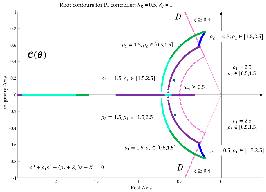
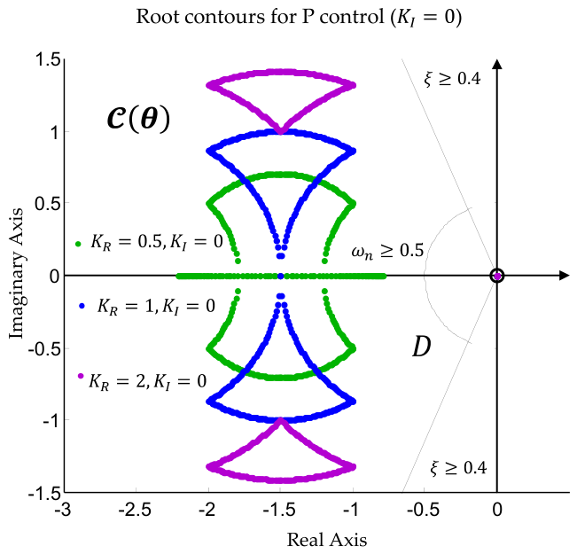
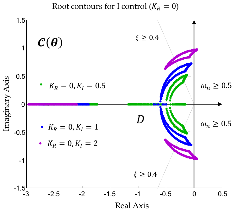
Figure 1 shows the contour $\mathcal{C}({\theta }^{*})$ for the nominal tuning ${\theta }^{*}=(K_R,K_I)=(0.5,1.0)$ and is used for a visual verification of the robust stability condition (22) and the robust admissibility condition (15). For comparison, Figure 2 and Figure 3 show the cases of P control $\left(K_I=0\right)$ and I control $\left(K_R=0\right)$, respectively.

For P control, the characteristic polynomial takes the form $p(s)=s\left[s^2+({\rho }_1+{\rho }_2)s+({\rho }_1{\rho }_2+K_R)\right],$ so that one pole remains at the origin. Therefore, the robust stability condition (22) is not satisfied in the strict sense. This case is nevertheless useful for evaluating the effect of the proportional term on the remaining poles.

For I control $\left(K_R=0\right)$, the fixed pole at the origin is no longer preserved. In the considered range of $K_I$, increasing the integral term leads to a more pronounced expansion of the contours along the imaginary axis and to a closer approach to the boundaries of the region $D$. This indicates a higher sensitivity of the oscillatory component to parametric uncertainty. The quantitative results for the P, I, and nominal PI controller cases are summarized in

Table 1. Quantitative assessment of root contours for P, I, and the nominal PI controller tuning.

Type	${\mathit{K}}_{\mathit{R}}$	${\mathit{K}}_{\mathit{I}}$	Robust Stability	Robust Admissibility	$\mathsf{\Delta }\mathit{\sigma }$(θ)	$\mathsf{\Delta }\mathit{\omega }$(θ)	${\mathit{d}}_{\mathit{m}\mathit{a}\mathit{x}}$(θ)	${\mathit{\mu }}_{\mathit{D}}$(θ)
PI	0.5	1.00	Yes	No	2.2574	1.5274	0.9136	-
P	0.50	0.00	No	No	2.2071	1.4142	0.8660	-
P	1.00	0.00	No	No	2.0000	2.0000	0.8660	-
P	2.00	0.00	No	No	2.0000	2.8284	0.5000	-
I	0.00	0.50	Yes	No	2.5286	1.0405	0.8154	-
I	0.00	1.00	Yes	No	2.7226	1.4526	0.6795	-
I	0.00	2.00	No	No	3.0105	1.9507	0.4405	-

The symbol “-” for ${\mu }_D(\theta )$ indicates that the corresponding tuning is not robustly admissible with respect to $D$; therefore, ${\mu }_D(\theta )$ is not interpreted as a positive geometric margin.

.

The results show that P control does not ensure strict robust stability, as, for $K_I=0$, one pole remains at the origin. For I control, the tunings $K_I=0.5$ and $K_I=1.0$ are robustly stable but not robustly admissible with respect to $D$, whereas for $K_I=2.0$ robust stability is also lost. The nominal PI tuning $\left(K_R,K_I)=(0.5,1.0\right)$ preserves robust stability but does not satisfy the robust admissibility condition (15). This confirms the distinction introduced in Section 2, whereby robust stability does not automatically guarantee robust admissibility with respect to the prescribed dynamic admissibility region $D$.

3.4. Quantitative Assessment of Root Contours

The nominal tuning ${\theta }^{*}=(0.5,1)$ is used as the starting point for the analysis under parametric uncertainty. For this tuning, as well as for the other candidate tunings considered, the root contours generated by admissible variations of the plant parameters $\rho \in {\mathsf{\Omega }}_{\rho }$ are constructed. The objective is to determine which tunings preserve not only robust stability in the sense of (22), but also robust admissibility with respect to the prescribed dynamic admissibility region $D$, i.e., satisfy condition (15).

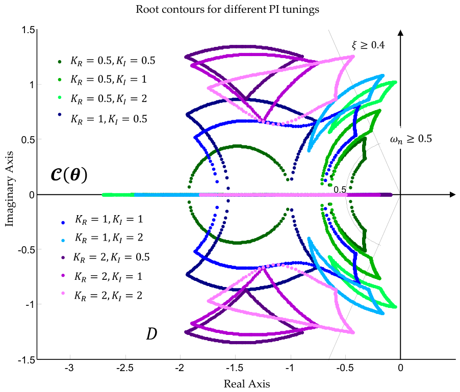
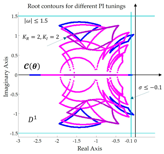
Figure 4 shows the root contours for nine candidate PI controller tunings. Each tuning $\theta =(K_R,K_I)$ generates its own set $\mathcal{C}(\theta )$, which describes the possible root locations under variations of the plant parameters within ${\mathsf{\Omega }}_{\rho }$ It can be seen from the figure that all considered tunings remain in the left half of the complex plane, which indicates robust stability. At the same time, none of the complete contours remains entirely within the prescribed dynamic admissibility region $D$. Thus, all nine tunings are robustly stable, but none are robustly admissible with respect to $D$.

For a quantitative comparison of the candidate tunings, the indices defined in (16)–(20) are computed. The first three indices evaluate the dispersion and sensitivity of the contours, whereas ${\mu }_D(\theta )$ is interpreted as a positive geometric margin only when the tuning is robustly admissible. The results obtained are summarized in

Table 2. Robust stability, robust admissibility, and quantitative root contour indices for candidate PI controller tunings.

${\mathit{K}}_{\mathit{R}}$	${\mathit{K}}_{\mathit{I}}$	Robust Stability	Robust Admissibility	$\mathsf{\Delta }\mathit{\sigma }$(θ)	$\mathsf{\Delta }\mathit{\omega }$(θ)	${\mathit{d}}_{\mathit{m}\mathit{a}\mathit{x}}$(θ)	${\mathit{\mu }}_{\mathit{D}}$(θ)
0.5	0.5	Yes	No	2.2106	1.0289	0.9250	-
0.5	1.0	Yes	No	2.2574	1.5274	0.9136	-
0.5	2	Yes	No	2.6489	2.0511	0.4206	-
1.0	0.5	Yes	No	1.8837	1.7347	1.1300	-
1.0	1.0	Yes	No	1.9114	1.6277	1.1776	-
1.0	2.0	Yes	No	2.2455	2.1640	0.5732	-
2.0	0.5	Yes	No	1.8608	2.6975	0.5360	-
2.0	1.0	Yes	No	1.6993	2.5534	0.5923	-
2.0	2.0	Yes	No	1.3830	2.5130	0.8172	-

The symbol “-” for ${\mu }_D(\theta )$ indicates that the corresponding tuning is not robustly admissible with respect to $D$; therefore, ${\mu }_D(\theta )$ is not interpreted as a positive geometric margin.

.

The numerical verification of each candidate tuning is performed according to the procedure described in Section 2.5. The numerical computations and simulations were performed using MATLAB R2013b (MathWorks, Natick, MA, USA). The uncertainty domain ${\mathsf{\Omega }}_{\rho }$ is discretized with a uniform step $h_{\rho }=0.02$, which corresponds to $N_1=N_2=51$ points for the parameters ${\rho }_1$ and ${\rho }_2$. The boundary trajectories used for visualization in Figure 1, Figure 2, Figure 3 and Figure 4 are obtained by varying one parameter while fixing the other one at a boundary value. However, the final verification of robust stability, robust admissibility, and the quantitative indices is performed on the full two-dimensional grid $51\times 51$, i.e., over 2601 combinations of $\left({\rho }_1,{\rho }_2\right)$, including both boundary and interior points.

Table 2 shows that all nine considered PI tunings are robustly stable. For all of them, condition (22) is satisfied, i.e., the roots remain in the left half of the complex plane under the admissible variations of the plant parameters. However, this is not sufficient to preserve the prescribed dynamic requirements, as none of the considered tunings satisfies the robust admissibility condition (15). For each tuning, at least part of the corresponding contour $\mathcal{C}(\theta )$ leaves the region $D$. Therefore, for the prescribed region $D$, the considered tuning grid, and the selected parametric uncertainty set, no tuning belonging to the set of robustly admissible solutions ${\Theta }_D^r$ is found.

The nominal tuning ${\theta }^{*}=(0.5,1.0)$ is also robustly stable, but it is not robustly admissible with respect to $D$. This confirms the main distinction introduced in Section 2—robust stability according to (22) does not automatically imply robust admissibility according to (15). In this case, the index ${\mu }_D(\theta )$ is not interpreted as a positive geometric margin for any of the candidate tunings; therefore, it is denoted by the symbol “-” in Table 2.

The analysis of the indices $\mathsf{\Delta }\sigma (\theta )$, $\mathsf{\Delta }\omega (\theta )$, and $d_{\mathrm{m}\mathrm{a}\mathrm{x}}(\theta )$ in Table 2 makes it possible to compare the sensitivity of the individual tunings to parametric uncertainty, even when none of the tunings is robustly admissible. A smaller value of $\mathsf{\Delta }\sigma (\theta )$ indicates lower dispersion of the roots along the real axis, whereas a smaller value of $\mathsf{\Delta }\omega (\theta )$ indicates lower dispersion along the imaginary axis. From this perspective, the tuning $\left(K_R,K_I)=(2.0,2.0\right)$ has the smallest horizontal dispersion, $\mathsf{\Delta }\sigma =1.3830$, whereas the tuning $\left(K_R,K_I)=(0.5,0.5\right)$ has the smallest vertical dispersion, $\mathsf{\Delta }\omega =1.0289$. However, these indices do not change the fact that condition (15) is not satisfied for any of the tunings considered.

Thus, the contour analysis has a diagnostic role in this example. It shows that the nominally selected tuning ${\theta }^{*}=(0.5,1.0)$, as well as the other considered PI tunings, ensures robust stability but not robust admissibility with respect to the prescribed region $D$. This means that achieving robust admissibility may require an extension of the set ${\mathsf{\Omega }}_{\theta }$, a modification of the prescribed region $D$, a reduction of the parametric uncertainty set ${\mathsf{\Omega }}_{\rho }$, or the selection of a different controller structure.

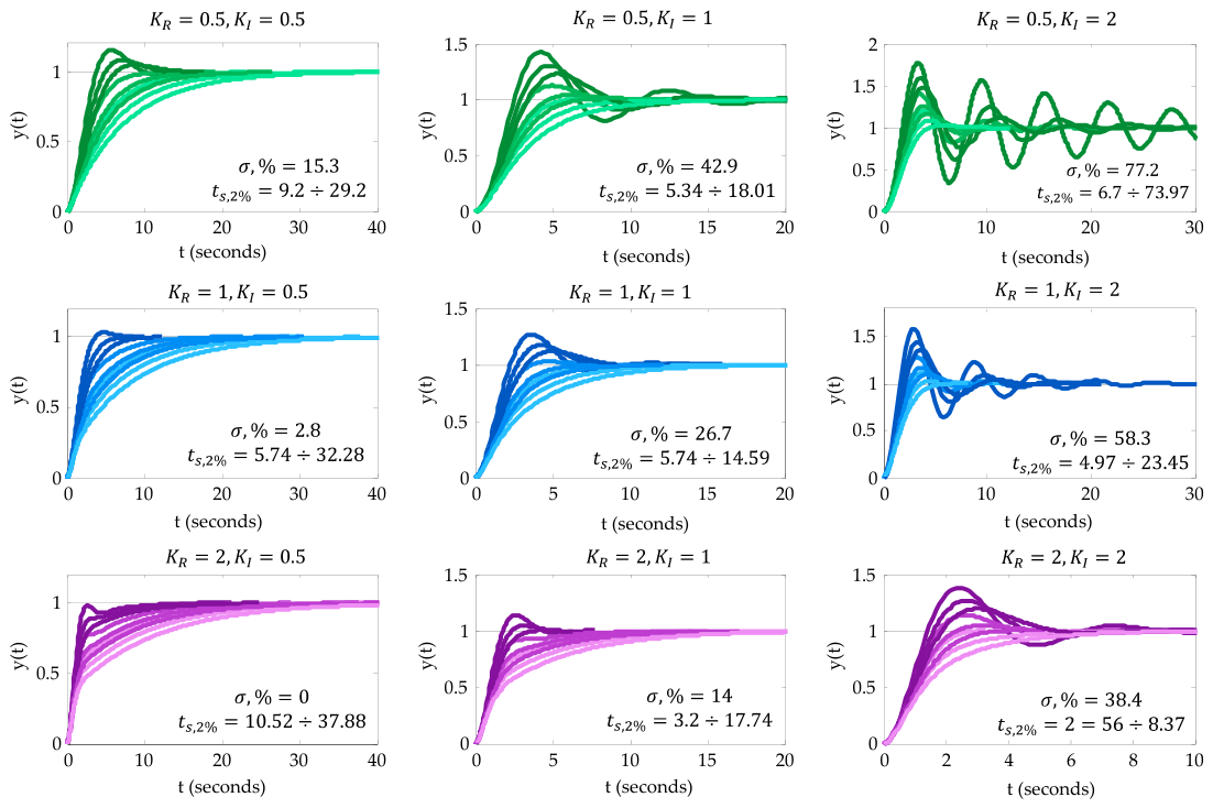
Additional information on the dynamic behavior of the control system is presented in Figure 5, which shows the step responses for the considered tunings under admissible variations of the plant parameters. These results complement the geometric interpretation provided by the root contours. Tunings whose contours lie closer to the boundary of $D$, or partially leave it, lead to more pronounced variations in the transient response, including larger overshoot, slower decay, or stronger sensitivity to parametric uncertainty. In the considered case, the absence of a tuning satisfying condition (15) means that none of the candidate tunings guarantees the prescribed dynamic admissibility for the entire set of parametric realizations under consideration.

In summary, the nominal tuning ${\theta }^{*}=(0.5,1.0)$ serves as the starting point and ensures robust stability, but it does not ensure robust admissibility with respect to the region $D$. For the considered grid of PI tunings, no tuning satisfying the condition $\mathcal{C}(\theta )\subset D$ is found. Therefore, in this example, the index ${\mu }_D(\theta )$ is not used to select among robustly admissible solutions; instead, the absence of a positive margin has a diagnostic meaning. The indices $\mathsf{\Delta }\sigma (\theta )$, $\mathsf{\Delta }\omega (\theta )$, and $d_{\mathrm{m}\mathrm{a}\mathrm{x}}(\theta )$ provide additional information on the sensitivity of the contours to parametric uncertainty.

The method has an important diagnostic value, because it makes it possible to determine not only which tuning is admissible, but also whether a robustly admissible tuning exists at all for the prescribed controller structure, uncertainty domain, and performance requirements. In the considered PI example, the results show that, although some tunings are robustly stable, the complete root contour does not remain inside the prescribed region $D$. This means that the desired transient performance cannot be guaranteed for all admissible plant-parameter variations only by changing the parameters $K_R$ and $K_I$.

After this diagnostic example, it is useful to consider a second situation in which several robustly admissible tunings exist. For this purpose, the admissibility region can be enlarged or defined according to more realistic engineering requirements, so that a selection between several tunings becomes possible. In this case, the proposed indices (16)–(20) can be used for comparison and selection of the most appropriate tuning.

3.5. Case with Selection Among Robustly Admissible PI Tunings

In this subsection, the admissibility region is defined by imposing constraints on the degree of stability and on the imaginary part of the poles. For a complex pole $s=\sigma +j\omega$, the region is defined as $D^1=\{s=\sigma +j\omega \in \mathbb{C}\mid \sigma \le -0.1,\mid \omega \mid \le 1.5\}.$ The first condition specifies a minimum degree of stability and ensures that the poles are located sufficiently far to the left of the imaginary axis. The second condition limits the oscillatory component of the transient response by restricting the imaginary part of the poles.

As the control plant, the uncertainty set, and the considered PI tunings are the same as in the previous example, the root contours do not change. Therefore, the indices $\mathsf{\Delta }\sigma$, $\mathsf{\Delta }\omega$, and $d_{\mathrm{m}\mathrm{a}\mathrm{x}}$, which characterize the size and displacement of the contours, keep the same values. Changing the admissibility region affects the robust admissibility classification and the geometric margin ${\mu }_D$, because they are evaluated with respect to the boundary of the new region $D^1$.

Figure 6 shows that, in addition to the complex-conjugate branches, some parts of the contours are also located on the real axis. These real poles are also included in the robust admissibility check. Therefore, a tuning is considered robustly admissible only if all branches of the contour, including those located on the real axis, remain inside the region $D^1$. This further restricts the number of admissible tunings, as shown in

Table 3. Robust stability, robust admissibility, and quantitative root contour indices for candidate PI controller tunings for admissibility region $D^1$.

${\mathit{K}}_{\mathit{R}}$	${\mathit{K}}_{\mathit{I}}$	Robust Stability	Robust Admissibility	$\mathsf{\Delta }\mathit{\sigma }$(θ)	$\mathsf{\Delta }\mathit{\omega }$(θ)	${\mathit{d}}_{\mathit{m}\mathit{a}\mathit{x}}$(θ)	${\mathit{\mu }}_{\mathit{D}}$(θ)
0.5	0.5	Yes	Yes	2.2106	1.0289	0.9250	0.0304
0.5	1.0	Yes	Yes	2.2574	1.5274	0.9136	0.0953
0.5	2.0	Yes	No	2.6489	2.0511	0.4206	-
1.0	0.5	Yes	Yes	1.8837	1.7347	1.1300	0.0163
1.0	1.0	Yes	Yes	1.9114	1.6277	1.1776	0.1662
1.0	2.0	Yes	Yes	2.2455	2.1640	0.5732	0.0653
2.0	0.5	Yes	No	1.8608	2.6975	0.5360	-
2.0	1.0	Yes	Yes	1.6993	2.5534	0.5923	0.1005
2.0	2.0	Yes	Yes	1.3830	2.5130	0.8172	0.2435

The symbol “-” for ${\mu }_D(\theta )$ indicates that the corresponding tuning is not robustly admissible with respect to $D^1$; therefore, ${\mu }_D(\theta )$ is not interpreted as a positive geometric margin.

.

It can be seen from Table 3 that, for the region $D^1$ defined by $\sigma \le -0.1$ and $\left|\omega \right|\le 1.5$, seven of the considered PI tunings are robustly admissible. This shows that, for a less restrictive admissibility region that is still justified from an engineering perspective, the proposed method can be used not only for diagnosis, but also for selection among several admissible tunings.

The tuning $\left(K_R,K_I)=(2,2\right)$ has the largest geometric margin with respect to the boundary of the region $D^1$, namely ${\mu }_D=0.2435$. In addition, it has the smallest dispersion along the real axis among the robustly admissible tunings, with $\mathsf{\Delta }\sigma =1.3830$. Therefore, the tuning $\left(K_R,K_I)=(2,2\right)$ is selected as the preferred one, as it provides the largest margin to the boundary of the admissible region and lower sensitivity of the decay rate to parametric uncertainty.

In Figure 6, the non-admissible tunings are shown in blue, the robustly admissible tunings are shown in pink, and the selected tuning $\left(K_R,K_I)=(2,2\right)$ is highlighted in a darker pink color.

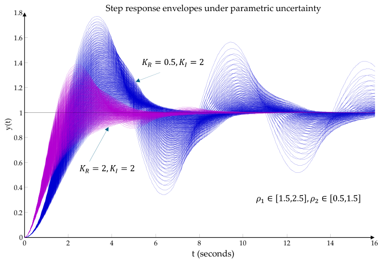
Additionally, to relate the geometric assessment to the behavior in the time domain, Figure 7 shows the transient responses for the selected robustly admissible tuning $\left(K_R,K_I)=(2,2\right)$ and for a tuning that does not satisfy the robust admissibility condition, namely $\left(K_R,K_I)=(0.5,2\right)$. For each of the two tunings, transient responses are computed under variation of the plant parameters within the prescribed uncertainty domain. The same color convention as in the contour plots is used: blue for the not robustly admissible tuning and dark pink for the selected tuning.

Figure 7 complements the contour analysis in Figure 6 by providing a comparison in the time domain between a not robustly admissible tuning and the selected robustly admissible tuning. The blue curves correspond to a tuning for which violation of the region $D^1$ leads to more pronounced oscillations and greater dispersion of the transient responses. For the selected tuning $\left(K_R,K_I)=(2,2\right)$, shown in dark pink, the transient responses are more compact and decay faster, which is consistent with the larger geometric margin ${\mu }_D$.

3.6. Robust Stability and Robust Admissibility Assessment

The geometric observations shown in Figure 2 and Figure 3 can be confirmed analytically using the Routh–Hurwitz criterion. For this purpose, the characteristic equation (36) is considered as a cubic polynomial with parametrically dependent coefficients: $p(s)=s^3+({\rho }_1+{\rho }_2)s^2+({\rho }_1{\rho }_2+K_R)s+K_I.$ For a cubic polynomial $s^3+a_1{s}^2+a_{2}s+a_3=0,$ the asymptotic stability conditions are $a_1>0,a_2>0,a_3>0,a_1{a}_2>a_3.$ In the considered case, $a_1={\rho }_1+{\rho }_2,a_2={\rho }_1{\rho }_2+K_R,a_3=K_I.$ Therefore, the stability conditions are as follows:

$${\rho }_1+{\rho }_2>0,{\rho }_1{\rho }_2+K_R>0,K_I>0,$$

(44)

$$({\rho }_1+{\rho }_2)({\rho }_1{\rho }_2+K_R)>K_I.$$

(45)

Under parametric uncertainty $\rho \in {\mathsf{\Omega }}_{\rho }$, these conditions must be satisfied for all admissible values of the plant parameters. For the considered intervals ${\rho }_1\in [1.5,2.5]$, ${\rho }_2\in [0.5,1.5]$, and for $K_R\ge 0$, the first two conditions in (44) are satisfied. The third condition requires $K_I>0$. The most restrictive condition is (45), as it relates the controller tunings to the most unfavorable values of the plant parameters.

Therefore, the robust stability condition can be written in terms of the worst-case value, as follows:

$$\underset{\rho \in {\mathsf{\Omega }}_{\rho }}{\mathrm{m}\mathrm{i}\mathrm{n}}\left[({\rho }_1+{\rho }_2)({\rho }_1{\rho }_2+K_R)\right]>K_I.$$

(46)

For the specified intervals and for $K_R\ge 0$, the minimum is attained at the lower bounds of the parameters:

$$\underset{\rho \in {\mathsf{\Omega }}_{\rho }}{\mathrm{m}\mathrm{i}\mathrm{n}}\left[({\rho }_1+{\rho }_2)({\rho }_1{\rho }_2+K_R)\right]=({\rho }_1^{-}+{\rho }_2^{-})({\rho }_1^{-}{\rho }_2^{-}+K_R).$$

(47)

Therefore, the robust stability boundary in the controller parameter plane is determined by (48), and the robustly stable region is given by (49).

$$K_I=({\rho }_1^{-}+{\rho }_2^{-})({\rho }_1^{-}{\rho }_2^{-}+K_R),$$

(48)

$$0<K_I<({\rho }_1^{-}+{\rho }_2^{-})({\rho }_1^{-}{\rho }_2^{-}+K_R).$$

(49)

For the specific values ${\rho }_1^{-}=1.5$ and ${\rho }_2^{-}=0.5$, one obtains the following:

$$0<K_I<1.5+2K_R.$$

(50)

The algebraic verification based on the Routh–Hurwitz criterion determines the set of robustly stable tunings, but it does not verify whether the poles remain inside the dynamic admissibility region $D$. Therefore, it serves as a first step, followed by the geometric verification of robust admissibility using condition (15). If this condition is satisfied, the corresponding tuning belongs to the set of robustly admissible tunings defined in (31). If (49) is satisfied but (15) is not, the tuning is robustly stable but does not guarantee preservation of the prescribed dynamic performance.

This distinction is observed in Table 2. All of the considered PI tunings are robustly stable, but none of them is robustly admissible with respect to $D$. In particular, the nominal tuning ${\theta }^{*}=(0.5,1)$ is robustly stable, but not robustly admissible. Therefore, for the considered grid of candidate tunings, the set ${\Theta }_D^r$ remains empty, i.e., no alternative tuning is selected from the robustly admissible set. In this case, the indices $\mathsf{\Delta }\sigma (\theta )$, $\mathsf{\Delta }\omega (\theta )$, and $d_{\mathrm{m}\mathrm{a}\mathrm{x}}(\theta )$ are used only to compare the sensitivity of the contours, whereas ${\mu }_D(\theta )$ is not interpreted as a positive geometric margin.

Thus, robust admissibility is not reduced to stability verification alone. It requires simultaneous satisfaction of the algebraic robust stability condition and the geometric condition requiring inclusion of the contour in the region $D$. This makes it possible to distinguish tunings that are only robustly stable from tunings that also preserve the prescribed dynamic requirements under uncertainty.

4. Comparative Discussion with Classical Robustness Tests

In this section, the proposed contour-based approach is compared with two classical types of verification D-decomposition in the controller parameter plane and frequency domain robustness conditions under a multiplicative uncertainty description. The aim is not to oppose these methods, but to clarify what type of information each of them provides.

4.1. Comparison with D-Decomposition

For comparison with the contour analysis, D-decomposition is considered in the controller parameter plane $\left(K_R,K_I\right)$.

For the system considered, the stability boundary is obtained by substituting $s=j\omega$ into the characteristic Equation (36): $s^3+({\rho }_1+{\rho }_2)s^2+({\rho }_1{\rho }_2+K_R)s+K_I=0.$ After substituting $s=j\omega$, one obtains $-j{\omega }^3-({\rho }_1+{\rho }_2){\omega }^2+j({\rho }_1{\rho }_2+K_R)\omega +K_I=0$.

Separating the real and imaginary parts leads to the following system:

$$\begin{gathered} K_I-\left({\rho }_1+{\rho }_2\right){\omega }^2=0, \\ -{\omega }^3+({\rho }_1{\rho }_2+K_R)\omega =0. \end{gathered}$$

For $\omega \ne 0$, the imaginary part gives $K_R(\omega )={\omega }^2-{\rho }_1{\rho }_2,$ whereas the real part gives $K_I(\omega )=({\rho }_1+{\rho }_2){\omega }^2$.

After eliminating $\omega$, the stability boundary for fixed values of the control plant parameters is obtained as follows:

$$K_I=({\rho }_1+{\rho }_2)(K_R+{\rho }_1{\rho }_2).$$

(51)

For the nominal model ${\rho }^{*}=(2,1)$, the nominal stability boundary is as follows:

$$K_I=\left(2+1\right)\left(K_R+2\cdot 1\right)=3K_R+6.$$

(52)

The obtained relation (52) coincides with the boundary case of the Routh–Hurwitz criterion for the considered third-order characteristic polynomial. For positive coefficients, the stability condition reduces to $({\rho }_1+{\rho }_2)({\rho }_1{\rho }_2+K_R)>K_I,$ and the boundary is obtained when equality holds.

In the presence of parametric uncertainty $\rho \in {\mathsf{\Omega }}_{\rho }$, a family of stability boundaries is obtained. The robustly stable region is determined as the intersection of the stability regions for all admissible values of the plant parameters.

As, for $K_R\ge 0$, the boundary $K_I=({\rho }_1+{\rho }_2)(K_R+{\rho }_1{\rho }_2)$ increases monotonically with respect to ${\rho }_1$ and ${\rho }_2$, the most restrictive boundary is obtained at the respective minimum values ${\rho }_1^{-}$ and ${\rho }_2^{-}$:

$$K_I=({\rho }_1^{-}+{\rho }_2^{-})(K_R+{\rho }_1^{-}{\rho }_2^{-}).$$

(53)

For the considered intervals, with ${\rho }_1^{-}=1.5$ and ${\rho }_2^{-}=0.5$, one obtains the following:

$$K_I=(1.5+0.5)(K_R+1.5\cdot 0.5)=2(K_R+0.75)=2K_R+1.5.$$

(54)

Therefore, the robustly stable region in the controller parameter plane is as follows:

$$0<K_I<2K_R+1.5.$$

(55)

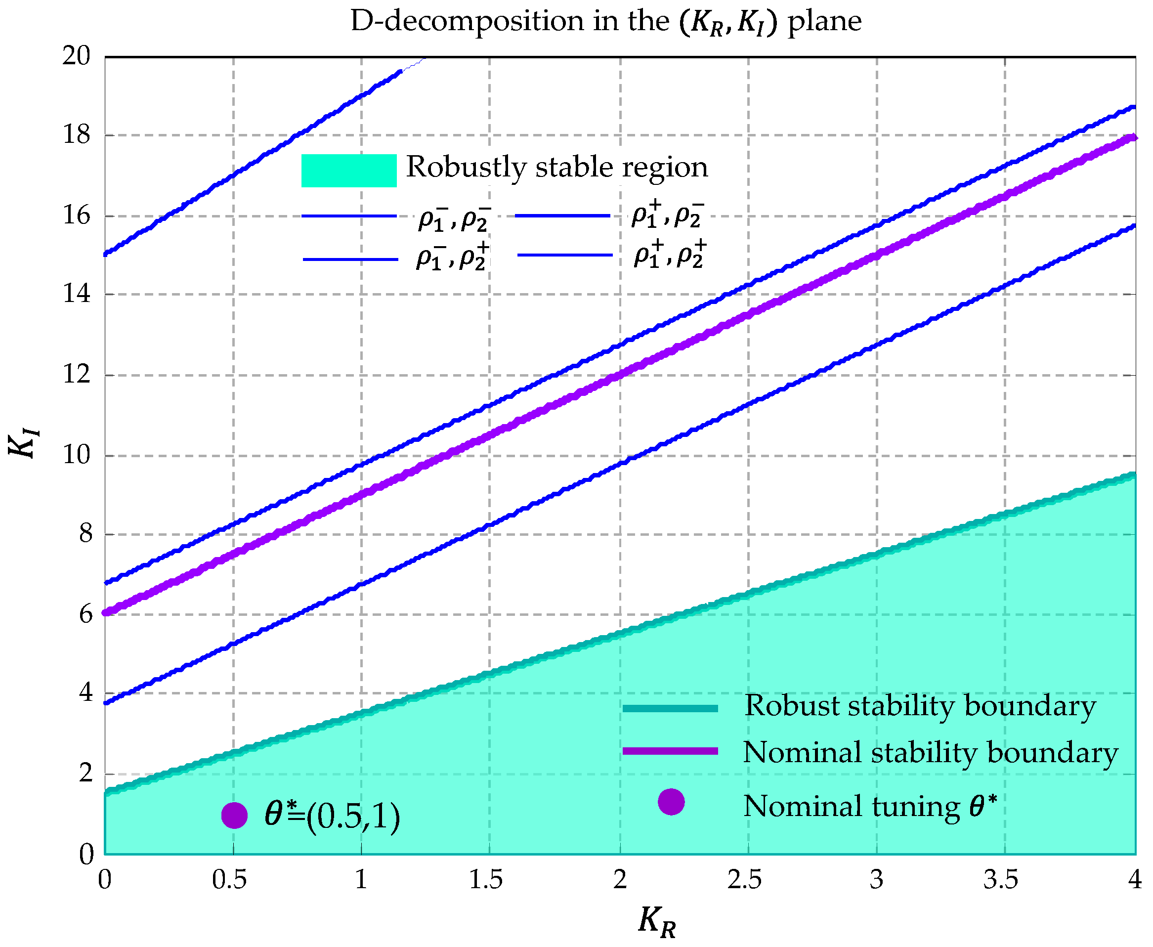
Figure 6 shows the D-decomposition in the $(K_R,K_I)$ plane.

The nominal stability boundary is given by the line $K_I=3K_R+6$, whereas the most restrictive robust stability boundary is given by $K_I=2K_R+1.5$.

The shaded region below the robust boundary and above the axis $K_I=0$ corresponds to condition (55). The point ${\theta }^{*}=(0.5,1.0)$ indicates the location of the selected nominal candidate tuning with respect to the robustly stable region.

Figure 8 shows that the nominal tuning ${\theta }^{*}=(0.5,1.0)$ lies inside the robustly stable region. This is also confirmed directly by (48), as $1.0<2\cdot 0.5+1.5=2.5$. Therefore, the tuning ${\theta }^{*}$ preserves stability for the considered interval family of plants.

D-decomposition provides an analytical boundary for robust stability in the controller parameter space. However, this condition does not guarantee satisfaction of the prescribed dynamic requirements, as it does not verify the location of the roots with respect to the dynamic admissibility region $D$. For robust admissibility, condition (15) must additionally be satisfied. Therefore, D-decomposition is used as an analytical verification of robust stability, whereas the root contours provide a geometric verification of robust admissibility under parametric uncertainty.

In other words, the two approaches are not interchangeable, but verify different properties of the closed-loop control system. D-decomposition does not distinguish between tunings whose poles remain stable but leave the region $D$, and tunings that preserve the prescribed dynamic requirements. This difference is captured by the contour analysis through ${\mu }_D(\theta )$ and the dispersion indices $\mathsf{\Delta }\sigma (\theta )$, $\mathsf{\Delta }\omega (\theta )$, and $d_{\mathrm{m}\mathrm{a}\mathrm{x}}(\theta )$, as shown in Table 2.

4.2. Comparison with Frequency Domain Conditions

For comparison with the contour analysis, classical frequency domain conditions for robust stability and robust performance are considered. The verification is performed for the nominal closed-loop control system obtained for $\rho ={\rho }^{*}$ and $\theta ={\theta }^{*}$. For the considered example, the nominal control plant is $G(s,\rho )={\displaystyle \frac{1}{\left(s+{\rho }_1)(s+{\rho }_2\right)}},$ and the nominal model corresponds to ${\rho }^{*}=(2,1)$. The nominal PI tuning ${\theta }^{*}=(K_R,K_I)=(0.5,1.0)$ is used.

The nominal open-loop transfer function is $L_0(s)=R(s,{\theta }^{*})G(s,{\rho }^{*}).$ The sensitivity and complementary sensitivity functions are $S_0(s)={\displaystyle \frac{1}{1+L_0(s)}},T_0(s)={\displaystyle \frac{L_0(s)}{1+L_0(s)}}.$ The parametric uncertainty in the plant is represented in multiplicative form as $G(s,\rho )=G(s,{\rho }^{*})[1+{\mathsf{\Delta }}_m(s,\rho )],$ where ${\mathsf{\Delta }}_m(s,\rho )={\displaystyle \frac{G(s,\rho )-G(s,{\rho }^{*})}{G(s,{\rho }^{*})}}.$ For the considered interval family, the frequency envelope of the multiplicative uncertainty is defined as $W_m(\omega )=\underset{\rho \in {\mathsf{\Omega }}_{\rho }}{\mathrm{m}\mathrm{a}\mathrm{x}}\left|{\mathsf{\Delta }}_m(j\omega ,\rho )\right|=\underset{\rho \in {\mathsf{\Omega }}_{\rho }}{\mathrm{m}\mathrm{a}\mathrm{x}}\left|{\displaystyle \frac{G(j\omega ,\rho )-G(j\omega ,{\rho }^{*})}{G(j\omega ,{\rho }^{*})}}\right|$.

The sufficient frequency domain condition for robust stability under multiplicative uncertainty has the following form:

$$\left|W_m(\omega )T_0(j\omega )\right|<1,\forall \omega .$$

(56)

In the considered case, the low-frequency deviation is determined by variations in both parameters ${\rho }_1$ and ${\rho }_2$, as $G(0,\rho )={\displaystyle \frac{1}{{\rho }_1{\rho }_2}},G(0,{\rho }^{*})={\displaystyle \frac{1}{{\rho }_1^{*}{\rho }_2^{*}}}={\displaystyle \frac{1}{2}}.$ Therefore, $W_m(0)=\underset{\rho \in {\mathsf{\Omega }}_{\rho }}{\mathrm{m}\mathrm{a}\mathrm{x}}\left|{\displaystyle \frac{G(0,\rho )-G(0,{\rho }^{*})}{G(0,{\rho }^{*})}}\right|=\underset{\rho \in {\mathsf{\Omega }}_{\rho }}{\mathrm{m}\mathrm{a}\mathrm{x}}\left|{\displaystyle \frac{2}{{\rho }_1{\rho }_2}}-1\right|.$ For ${\rho }_1\in [1.5,2.5]$ and ${\rho }_2\in [0.5,1.5]$, the product ${\rho }_1{\rho }_2$ takes values in the interval $\left[0.75,3.75\right]$. Hence, $W_m(0)=\mathrm{m}\mathrm{a}\mathrm{x}\left\{\left|{\displaystyle \frac{2}{0.75}}-1\right|,\left|{\displaystyle \frac{2}{3.75}}-1\right|\right\}=\mathrm{m}\mathrm{a}\mathrm{x}\{1.6667,0.4667\}=1.6667.$ As ${\mathrm{T}}_0(0)=1$ for the nominal closed-loop control system with the PI controller, it follows that $\left|W_m(0)T_0(0)\right|=1.6667>1.$ Therefore, the strict condition (56) is not satisfied in the low-frequency range.

This shows that the selected multiplicative uncertainty description does not allow robust stability to be confirmed by the sufficient small-gain condition. This violation should not be interpreted as proof of instability of the specific parametric family, but rather as the inability of the selected sufficient condition to confirm robust stability under the adopted multiplicative uncertainty description.

To assess performance, a weighting function $W_p(s)$ is introduced to specify a requirement on the sensitivity function $S_0(s)$. For an illustrative verification, $W_p(s)=1/s$ is used, emphasizing the low-frequency behavior of the sensitivity function. The nominal performance condition is as follows:

$$\left|W_p(j\omega )S_0(j\omega )\right|<1,\forall \omega .$$

(57)

When the performance requirement and the multiplicative uncertainty are considered simultaneously, the sufficient SISO condition for robust performance can be written as follows:

$$\left|W_p(j\omega )S_0(j\omega )\right|+\left|{ W}_m(\omega )T_0(j\omega )\right|<1,\forall \omega .$$

(58)

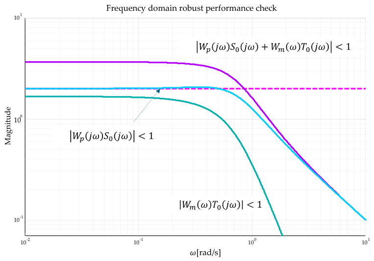
Figure 9 presents a graphical visualization of (56)–(58).

The condition $\left|W_p(j\omega )S_0(j\omega )\right|+\left|{ W}_m(\omega )T_0(j\omega )\right|<1$ is violated in the low-frequency range. Figure 9 shows that the frequency domain conditions (56) and (58) are not satisfied for the selected multiplicative uncertainty description. This does not contradict the results of the parametric verification obtained through D-decomposition and contour analysis.

Condition (56) is a sufficient, but not necessary, condition for robust stability. When the frequency envelope $W_m(\omega )$ is used, the parametric structure of the uncertainty is represented by the maximum magnitude of the relative deviation. As a result, information about the dependence between the parameters and the specific way in which they enter the characteristic polynomial is lost.

The contour-based approach preserves this structure, as it works directly with $p(s,\theta ,\rho )=0$ and tracks the root locations for the admissible parameter values.

Therefore, the frequency domain analysis and the contour-based approach provide different types of information. Conditions (56) and (58) represent sufficient frequency domain checks for robust stability and robust performance under multiplicative uncertainty. In contrast, condition (15) verifies robust admissibility through the location of the possible roots in the complex s-plane. This makes it possible to distinguish tunings that are robustly stable from tunings that also preserve the prescribed dynamic requirements.

4.3. Additional Validation Examples

As an additional validation of the proposed contour-based approach, two examples with different levels of complexity are considered. The first-order aperiodic element with a P controller and one uncertain parameter, and a higher-order system with a PID controller and three uncertain plant parameters.

The aim is to show that the procedure is applicable both to a one-parameter root trajectory and to contours formed by multiple boundary trajectories. In addition, it is verified whether the indices $\mathsf{\Delta }\sigma$, $\mathsf{\Delta }\omega$, $d_{\mathrm{m}\mathrm{a}\mathrm{x}}$, and ${\mu }_D$ can be used to compare candidate tunings.

4.3.1. Example 1: First-Order Plant with P Controller

A first-order aperiodic element is considered, $G_1(s,T)={\displaystyle \frac{k_G}{Ts+1}},$ where $T$ is an uncertain parameter. The nominal value $T^{*}=1$, the gain $k_G=2$, and the uncertainty interval $T\in [0.7,1.3]$ are used. With a P controller $R_1(s,K_R)=K_R$ and unity negative feedback, the characteristic equation is $Ts+1+K_R{k}_G=0,$ from which $s(T)=-{\displaystyle \frac{1+K_R{k}_G}{T}}$ is obtained. For a fixed value of $K_R$ and $T\in [0.7,1.3]$, the one-parameter trajectory is obtained as ${\mathcal{C}}_1(K_R)=\{s(T)\in \mathbb{C}\mid T\in [0.7,1.3\left]\right\}$.

The performance region is defined as $D_1=\{s\in \mathbb{C}\mid -8\le Re(s)\le -2\}$.

Robust admissibility is verified by the condition ${\mathcal{C}}_1(K_R)\subset D_1$.

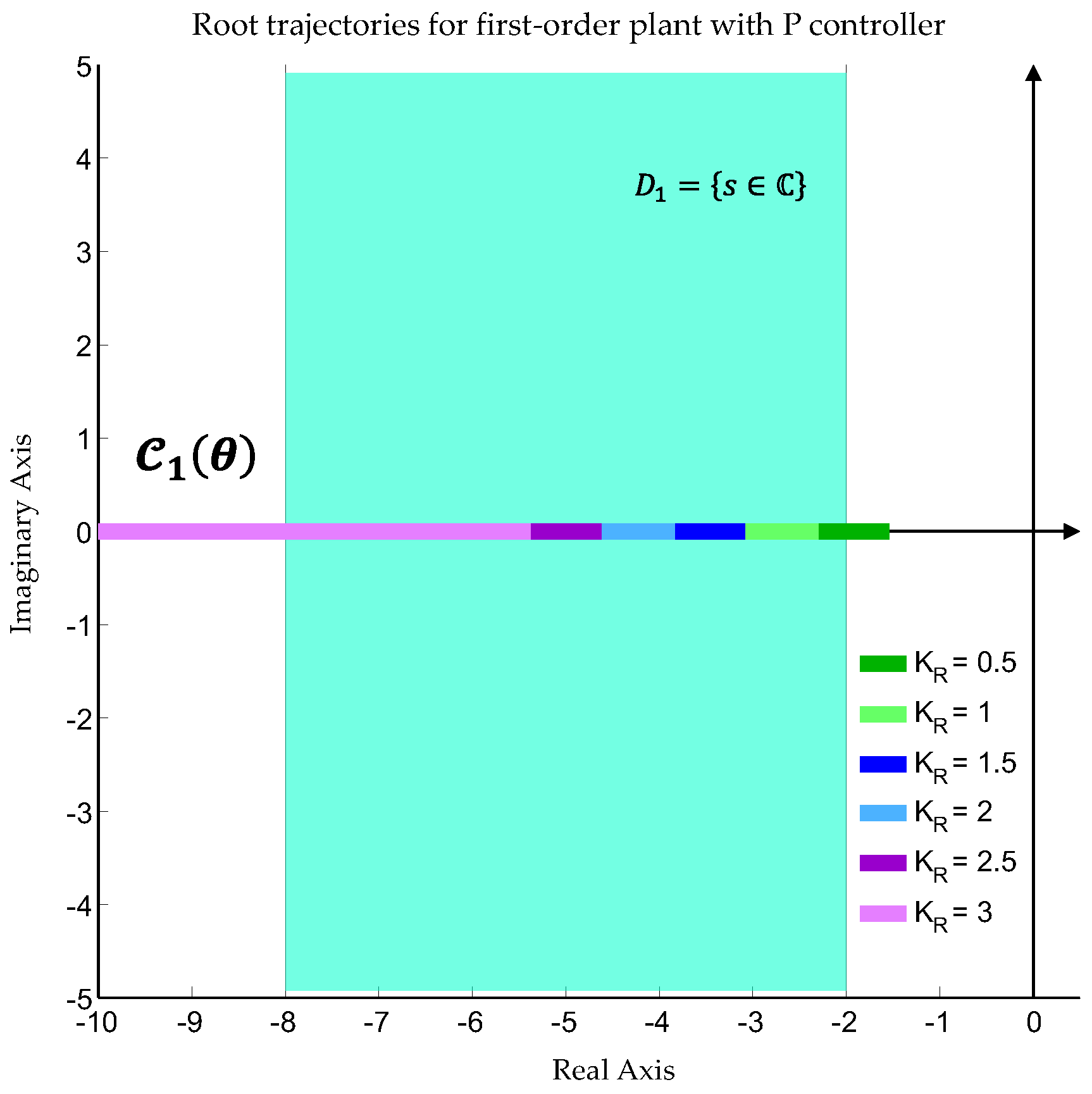
Figure 10 shows that all considered P tunings are robustly stable, as the trajectories remain in the left half of the complex s-plane.

The difference between them appears with respect to the region $D_1$. For small values of $K_R$, the trajectory remains too close to the imaginary axis, whereas for large values, part of it moves beyond the left boundary of $D_1$. Therefore, even for a first-order control system, robust stability and robust admissibility are distinct properties.

4.3.2. Higher-Order Plant with PID Controller [6]

As a second example, a higher-order system is considered, $G_2(s,\rho )={\displaystyle \frac{k_G}{s({\tau }_{1}s+1)({\tau }_{2}s+1)}},$ where $\rho =[{\tau }_1,{\tau }_2,k_G{]}^T$. The nominal values are ${\tau }_1^{*}=0.3$, ${\tau }_2^{*}=0.2$, and $k_G^{*}=1.6$, while the parametric uncertainty is defined by intervals of $\pm 10\%$ around the nominal values. A PID controller is used, $R_2(s,\theta )=K_R+{\displaystyle \frac{K_I}{s}}+K_{D}s,\theta =[K_R,K_I,K_D{]}^T.$

The central candidate tuning is selected as ${\theta }_2^{*}=[4.16,0.0416,1{]}^T,$ and additional tunings obtained by $\pm 20\%$ variation of the individual controller parameters are also considered.

The characteristic polynomial of the closed-loop control system is $P_2(s,\theta ,\rho )={\tau }_1{\tau }_2{s}^4+({\tau }_1+{\tau }_2)s^3+(1+k_G{K}_D)s^2+k_G{K}_{R}s+k_G{K}_I.$ For each fixed tuning $\theta$, only the plant parameters ${\tau }_1$, ${\tau }_2$, and $k_G$ are varied.

As the number of uncertain parameters is $m=3$, the number of boundary trajectories is $N_{gr}=3\cdot 2^{3-1}=12$.

These trajectories form an approximate estimate of the contour ${\mathcal{C}}_2(\theta )$. The performance region is defined as $D_2=\{s\in \mathbb{C}\mid 0.3\le \xi (s)\le 0.5,1.5\le -Re(s)\le 2.5\}.$ Robust admissibility is verified by the condition ${\mathcal{C}}_2(\theta )\subset D_2.$

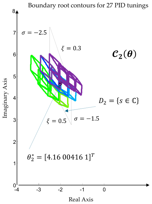
Figure 11 shows that the obtained root sets remain in the left half of the complex s-plane, but some of the boundary trajectories are close to the boundaries of $D_2$ or leave this region. Therefore, the considered tunings may be robustly stable without satisfying the strict robust admissibility condition with respect to the selected performance region.

Table 4. Quantitative root contour indices for the additional validation examples.

System/Controller	Uncertain Parameters	Tuning	${\mathit{N}}_{\mathit{g}\mathit{r}}$	Robust Stability	Robust Admissibility	$\mathsf{\Delta }\mathit{\sigma }(\mathit{\theta })$	$\mathsf{\Delta }\mathit{\omega }\left(\mathit{\theta }\right)$	${\mathit{d}}_{\mathit{m}\mathit{a}\mathit{x}}(\mathit{\theta })$	${\mathit{\mu }}_{\mathit{D}}\left(\mathit{\theta }\right)$	Main Conclusion
First-order plant + P	$T\in [0.7,1.3]$	$K_R=0.5$	1	Yes	No	1.3187	0.0000	0.8571	—	Stable tuning, but the contour leaves $D_1$ to the right
First-order plant + P	$T\in [0.7,1.3]$	$K_R=1.5$	1	Yes	Nes	2.6374	0.0000	1.7143	1.0769	Largest margin among the robustly admissible P tunings
First-order plant + P	$T\in [0.7,1.3]$	$K_R=3$	1	Yes	No	4.6154	0.0000	3.0000	—	Stable tuning, but the contour leaves $D_1$ to the left
Higher-order plant + PID	${\tau }_1,{\tau }_2,$ $k_G\pm 10\%$	${\theta }_2*$	12	Yes	No	4.4286	10.8020	0.8726	—	Stable tuning, but the strict inclusion in $D_2$ is not satisfied
Higher-order plant + PID	${\tau }_1,{\tau }_2,$ $k_G\pm 10\%$	$K_{D-20\%}$	12	Yes	No	5.3218	9.9054	0.7130	—	Smaller $d_{\mathrm{m}\mathrm{a}\mathrm{x}}(\theta )$, but the tuning remains inadmissible with respect to $D_2$
Higher-order plant + PID	${\tau }_1,{\tau }_2,$ $k_G\pm 10\%$	$K_{D+20\%}$	12	Yes	No	3.5835	11.9168	1.0059	—	Smaller $\mathsf{\Delta }\sigma$, but larger vertical dispersion

The symbol “-” for ${\mu }_D(\theta )$ indicates that the corresponding tuning is not robustly admissible with respect to $D$; therefore, ${\mu }_D(\theta )$ is not interpreted as a positive geometric margin.

shows that, in both additional examples, robust stability and robust admissibility are clearly distinguished. For the first-order control system, all considered P tunings are robustly stable, but only some of them are robustly admissible with respect to $D_1$. The tuning $K_R=1.5$ has the largest margin among the robustly admissible tunings, ${\mu }_D=1.0769$, whereas $K_R=0.5$ and $K_R=3.0$ illustrate the two types of violation of the region $D_1$, respectively to the right and to the left of the admissible interval.

In the PID example, the representative tunings are also robustly stable, but the strict condition ${\mathcal{C}}_2(\theta )\subset D_2$ is not satisfied for the cases shown. This does not weaken the contour-based approach but rather demonstrates its diagnostic role. The method not only confirms stability but also indicates when the prescribed performance region is too restrictive for the selected controller structure, the admissible tuning set, or the considered parametric uncertainty.

Table 5. Comparative robustness checks for the additional validation examples.

Example	Analytical Check/D-Decomposition	Frequency Domain Check	Interpretation
Example 1	D-decomposition is not required. From the explicit expression $s\left(T\right)=-{\displaystyle \frac{1+K_R{k}_G}{T}}$ it follows that for $T>0$, $k_G>0 \mathrm{a}\mathrm{n}\mathrm{d}$ $K_R>0$ the pole remains in the left half of the complex plane.	For the nominal tuning $K_R^{*}=2;$ $\left|W_m(\omega )T_0(j\omega )\right|\approx 0.26<1$ ⇒ robust stability: yes; $\left|W_p\left(j\omega \right)S_0\left(j\omega \right)\right|+$ $\left|W_m\left(\omega \right)T_0\left(j\omega \right)\right|\approx 4>1$ ⇒ robust performance: no.	Stability and performance are different properties: all tunings are stable, but only some of them are robustly admissible with respect to $D_1$.
Example 2	D-decomposition in the ($K_R-K_I$) plane for fixed $K_D=1$ shows that the nominal PID tuning lies inside the robust stability region.	For the nominal PID tuning ${\theta }_2*:$ $\left|W_m(\omega )T_0(j\omega )\right|\approx 0.35<1$ ⇒robust stability: yes; $\left|W_p\left(j\omega \right)S_0\left(j\omega \right)\right|+\left|W_m\left(\omega \right)T_0\left(j\omega \right)\right|\approx 0.65<1$ ⇒ robust performance: yes.	The frequency-domain check confirms the sufficient conditions, but the root contour analysis shows that the strict geometric inclusion $C_2(\theta )\subset D_2$ is not satisfied.

complements the contour-based assessment through analytical/D-decomposition and frequency domain verification. In the first-order example, stability is proven directly from the explicit pole expression, and the frequency domain verification confirms robust stability but not the selected robust performance condition. In the PID example, D-decomposition and the frequency domain conditions confirm stability, whereas the contour analysis shows that the pole sets do not remain entirely inside the prescribed region $D_2$. This indicates that frequency domain conditions and contour analysis are not interchangeable checks but evaluate different forms of robust performance.

The two examples illustrate different levels of complexity of the proposed procedure. For the aperiodic element with one uncertain parameter, ${\mathcal{C}}_1(K_R)$ reduces to a one-parameter root trajectory, whereas for the PID-controlled system with three uncertain parameters, ${\mathcal{C}}_2(\theta )$ is formed by 12 boundary trajectories for each tuning. In both cases, contour analysis distinguishes tunings that are only robustly stable from tunings that preserve the prescribed dynamic performance. The indices $\mathsf{\Delta }\sigma$, $\mathsf{\Delta }\omega$, $d_{\mathrm{m}\mathrm{a}\mathrm{x}}$, and ${\mu }_D$ complement the visual assessment and allow candidate tunings to be compared in terms of dispersion, sensitivity, and margin.

5. Discussion

D-decomposition, frequency domain conditions, and contour analysis verify different properties of the closed-loop control system. Therefore, their results have different interpretations. D-decomposition is performed in the controller parameter space $(K_R,K_I)$. In this approach, the controller parameters are treated as free coordinates, and the condition for the existence of roots on the imaginary axis, $s=j\omega$, determines the boundaries between regions with different numbers of roots in the left and right half-planes. For the control system considered, these boundaries are given by the relation derived in (51). Under parametric uncertainty $\rho \in {\mathsf{\Omega }}_{\rho }$, a family of such boundaries is obtained, and the robustly stable region is determined as the intersection of the stability regions for all admissible values of the control plant parameters. In the present case, this leads to the robust stability condition given in (55). Thus, D-decomposition determines a set of robustly stable controller tunings, after which a specific tuning $\theta$ is verified by checking its membership in this set.

Root-contour analysis is performed in the complex s-plane. In this approach, for each fixed controller tuning $\theta =[K_R,K_I{]}^T$, the control plant parameters $\rho \in {\mathsf{\Omega }}_{\rho }$ are varied, resulting in the set of possible root locations $\mathcal{C}(\theta )$. This set is defined in (6) and describes the possible root locations in the complex s-plane. Unlike D-decomposition, which verifies only whether the roots remain in the left half-plane, contour analysis makes it possible to verify whether all possible root locations lie inside the prescribed dynamic admissibility region $D$. The region $D$ is defined in general form in (11) and specified for the considered example in (35), while robust admissibility is verified using condition (15). Therefore, root contours verify not only robust stability, but robust admissibility with respect to the prescribed dynamic requirements. For this reason, tuning may be robustly stable according to D-decomposition, but not robustly admissible with respect to $D$, if part of the contours leaves the dynamic admissibility region.

Frequency domain robust analysis with multiplicative uncertainty is performed using the nominal closed-loop control system and a selected frequency domain description of the uncertainty. In the case considered, the sufficient conditions for robust stability and robust performance, given in (56) and (58) respectively, are not satisfied. This does not mean that the specific interval family is unstable. The results obtained from D-decomposition and contour analysis show that the selected tuning can preserve stability under the considered parametric uncertainty. The reason is that the small-gain condition is sufficient, but not necessary, for robust stability. It accounts for a broader class of multiplicative uncertainties and may therefore be more conservative than the parametric verification based on the characteristic polynomial.

Therefore, the approaches considered have different roles in the process of controller design and verification. D-decomposition determines the robustly stable region in the controller parameter space and makes it possible to establish whether a given tuning belongs to a set of stable solutions. However, it does not provide direct information on whether the roots satisfy the prescribed dynamic requirements. Frequency domain small-gain analysis provides a classical sufficient check for robust stability and robust performance, but, in the presence of large low-frequency multiplicative uncertainty, it may be conservative and may fail to confirm stability even when parametric analysis proves it.

In this context, the proposed approach, based on parametric trajectories used to obtain root contours, plays an intermediate and practically useful role. It works directly with the parametric characteristic Equation (4) and preserves information about the structure of the uncertainty. This enables a geometric verification of whether, under parametric uncertainty, all possible root locations remain inside the dynamic admissibility region $D$.

From an engineering point of view, the advantage of contour analysis is that it shows not only whether the system remains stable, but also how the pole locations change under parametric uncertainty. This enables a direct assessment of the possible degradation of dynamic indicators such as damping, natural frequency, and response speed. The introduced indices $\mathsf{\Delta }\sigma (\theta )$, $\mathsf{\Delta }\omega (\theta )$, $d_{\mathrm{m}\mathrm{a}\mathrm{x}}(\theta )$, and ${\mu }_D(\theta )$, defined in (16)–(20), complement the visual analysis by providing a quantitative assessment of the contour dispersion and margin. When robustly admissible tunings exist, these indices allow them to be ranked according to sensitivity and geometric margin. When no such tuning is found, as in the main PI example, the same indices have a diagnostic role and indicate the degree of root dispersion with respect to the prescribed region $D$.

In the main PI example, the candidate tunings considered are robustly stable, but none of them is robustly admissible with respect to the prescribed region $D$. Thus, contour analysis does not select a tuning from ${\Theta }_D^r$, but identifies that no robustly admissible solution is found for the prescribed PI controller structure, tuning grid, admissibility region, and uncertainty set.

The absence of a robustly admissible tuning should not be regarded as a weakness of the method, but rather as a diagnostic result for the considered controller tuning problem. It shows that, for the prescribed requirements and the considered set of tunings, robust stability is not sufficient to guarantee the desired dynamic performance. The additional example with the region $D^1$ illustrates the other possible situation, where several robustly admissible tunings exist and the proposed indices can be used for a justified selection among them.

A similar distinction is observed in the additional validation examples. For the first-order control plant with a P controller, all considered tunings are stable, but only some satisfy the prescribed performance region $D_1$. For the higher-order PID-controlled system, robust stability again does not guarantee satisfaction of the stricter condition ${\mathcal{C}}_2(\theta )\subset D_2$.

From an engineering point of view, this result indicates that, when no tuning satisfies $\mathcal{C}(\theta )\subset D$, the controller structure, admissible tuning range, performance region, or uncertainty description should be reconsidered.

The main differences between the approaches considered are summarized in

Table 6. Comparison of D-decomposition, frequency domain conditions, and root contour analysis.

Approach	Analysis Domain	Main Condition	What It Checks	Main Advantage	Limitation
D-decomposition	Parameter space ($K_R,K_I$)	$K_I=({\rho }_1+{\rho }_2)(K_R+{\rho }_1{\rho }_2)$ $0<K_I<2K_R+1.5$	Robust stability	Provides an analytical stability boundary	Does not verify the performance region $D$
Frequency domain conditions	Frequency domain	$\left|W_m(\omega )T_0(j\omega )\right|<1$ $\left|W_p\left(j\omega \right)S_0\left(j\omega \right)\right|+\left|W_m\left(\omega \right)T_0\left(j\omega \right)\right|<1$	Sufficient conditions for robust stability and robust performance	Classical frequency domain framework for robustness analysis	May be conservative under a multiplicative uncertainty description
Root contour analysis	Complex $s$-plane	$\mathcal{C}(\theta )\subset D$	Robust admissibility with respect to the dynamic performance requirements	Provides a direct geometric link between uncertainty and pole locations	Depends on the construction/discretization of the root contours

. It is important to emphasize that these approaches are not interchangeable. D-decomposition provides an analytical region of robust stability, frequency domain conditions provide a sufficient verification under the selected uncertainty description, and contour analysis verifies the geometric inclusion of the pole sets in the dynamic admissibility region $D$. Therefore, their combined use provides a more complete picture of stability, dynamic performance, and the possible conservativeness of different uncertainty descriptions.

Therefore, the proposed procedure uses root contours to verify robust admissibility with respect to the prescribed performance region, whereas D-decomposition and frequency domain conditions are used as comparative criteria for assessing robust stability and the conservativeness of the selected frequency domain uncertainty description, respectively.

In the proposed procedure, the controller tuning $\theta$ is fixed, while the contour $\mathcal{C}(\theta )$ is generated by the variation of the uncertain plant parameters $\rho \in {\mathsf{\Omega }}_{\rho }$. Therefore, increasing the number of uncertain parameters does not change the principle of the method, but it increases the number of boundary trajectories used for visualizing the parametrically induced set of pole locations. For $m$ uncertain parameters, the number of these trajectories is $m{2}^{m-1}$, which means that, for higher-dimensional uncertainty, complete visualization may become cluttered. In such cases, the boundary trajectories can be used selectively to present critical sections, while the final verification of robust admissibility is performed numerically over the discretized set ${\mathsf{\Omega }}_{\rho }^N$ using the condition ${\mathcal{C}}_N(\theta )\subset D$. Thus, the method remains applicable as a numerical procedure for verification and comparison of fixed candidate tunings, whereas visualization has a supporting interpretative role.

The present formulation is oriented toward linear continuous-time SISO control systems, for which the characteristic equation is represented as a polynomial in the s-plane. For discrete-time systems, the main idea is preserved, but the admissibility region should be defined in the z-plane, and the stability condition should be related to the location of the roots with respect to the unit circle. For multiple input–multiple output control (MIMO) systems, direct application is more complex, as the set of eigenvalues or the characteristic polynomial of the closed-loop system must be analyzed.

6. Conclusions

This study proposed a geometric procedure for verifying and selecting candidate controller tunings under parametric uncertainty. The approach combines parametrically induced root trajectories with contour analysis of the possible pole locations generated by admissible variations of the plant parameters. In this way, the robust verification problem is considered directly in the complex s-plane, where the pole locations are compared with a prescribed dynamic admissibility region $D$.

The results obtained show that nominally admissible tuning does not automatically guarantee robust admissibility. Using root contours, it is possible to verify whether the set $\mathcal{C}(\theta )$ remains inside the prescribed region $D$, which enables a distinction between robust stability and preservation of dynamic performance. For this purpose, the set-inclusion condition $\mathcal{C}(\theta )\subset D$ is used as a geometric criterion for robust admissibility.

In the main PI example, the considered candidate tunings preserve robust stability but do not satisfy the stricter robust admissibility condition with respect to $D$. This confirms that robust stability and robust admissibility are not equivalent and shows that the proposed procedure can identify cases in which no tuning satisfying $\mathcal{C}(\theta )\subset D$ is found within the prescribed tuning grid.

The comparison with D-decomposition shows that this classical parametric approach provides an analytical boundary for robust stability, whereas contour analysis provides additional information about the location of the roots with respect to the dynamic requirements. The frequency domain conditions for robust stability and robust performance serve as a comparative framework and, in the considered example, indicate possible conservativeness under the multiplicative description of parametric uncertainty. Therefore, the approaches considered are not interchangeable, but complement each other in the assessment of stability, dynamic performance, and the influence of uncertainty.

The main advantage of the proposed approach is the direct geometric interpretation of the influence of the parameters on the closed-loop roots. This makes it suitable for preliminary engineering tuning, selection of candidate parameters, and visual assessment of sensitivity to uncertainty. The introduced quantitative indices $\mathsf{\Delta }\sigma (\theta )$, $\mathsf{\Delta }\omega (\theta )$, $d_{\mathrm{m}\mathrm{a}\mathrm{x}}(\theta )$, and ${\mu }_D(\theta )$ complement the visual verification by enabling assessment of the size, dispersion, and margin of the contours with respect to the region $D$.

When robustly admissible tunings are available, these indices can be used to select among them. When no robustly admissible tuning is found, as in the main PI example, the indices have diagnostic value and indicate the need to modify ${\mathsf{\Omega }}_{\theta }$, $D$, ${\mathsf{\Omega }}_{\rho }$, or the controller structure.

The additional validation examples show that the procedure can be applied both to low-order single-parameter control systems and to more complex models with several uncertain parameters. In the first-order example, the contour reduces to a one-parameter root trajectory, whereas in the PID-controlled system with three uncertain parameters, the contours are formed by multiple boundary trajectories. In both cases, the approach makes it possible to distinguish tunings that are only robustly stable from tunings that preserve the prescribed dynamic performance.

The limitations of the approach are related to the assumptions required for constructing root contours. The method is most directly applicable to SISO linear continuous-time control systems for which the characteristic equation can be represented in polynomial form, and the considered parameters can be explicitly separated in it. For parameters entering in a nonlinear or irrational form, for sign changes of the varied parameter, and for time-delay systems, modified constructions, direct numerical root tracking, or additional analytical and frequency domain methods are required.

Future work may include the automated generation of admissibility regions, extension to more general classes of uncertainty, and the use of the obtained admissible and robustly admissible tuning sets as a formalized basis for intelligent procedures for robust tuning, selection, and adaptation of controller parameters. The extension of the proposed approach to discrete-time and MIMO systems also requires a separate formulation and is considered as a direction for future work.