A New Hyperbolic PID-Type Control Scheme for a Direct-Drive Pendulum

Abstract

This paper addresses the position control problem for a Lagrangian pendulum. Using a strict Lyapunov function, a rigorous analysis is presented to prove that the closed-loop system equilibrium point composed of the pendulum dynamics and a classical linear PID control is globally asymptotically stable. Motivated by these results, the theoretical proposal is extended to analyze a novel hyperbolic PID-type control scheme; reformulating the Lyapunov function, global asymptotic stability of the equilibrium point for the corresponding closed-loop equation is demonstrated. The proposed hyperbolic scheme is a rational function with bounded control action composed of a suitable combination of hyperbolic sine and cosine functions. The hyperbolic structure is used in the proportional, integral, and derivative terms of the control algorithm to drive the position error and joint velocity to zero. Experimental results of both a linear PID and a novel hyperbolic PID-type controller on a direct-drive pendulum are presented to illustrate the effectiveness and performance of the proposed control algorithm.

1. Introduction

The proportional-integral-derivative (PID) controller is one of the most widely used strategies for controlling dynamic systems, due to its simple structure and satisfactory performance in a variety of applications [1,2,3,4]. Since its invention in 1911 by Elmer Sperry [5], the PID algorithm has been known to offer one of the simplest yet effective solutions for regulation problems. However, it was not until 1922 that the first theoretical analysis was developed by Russian-American engineer Nicolas Minorsky [6]. Because of its simplicity and ease of implementation, PID control has gained widespread acceptance in both academia and industry [7].

There has been a recent increase in PID applications, spanning domains such as industrial processes, aerospace, energy systems, and mechatronic devices. Although PID control is linear in structure, it is commonly used in nonlinear Lagrangian systems of practical relevance, such as mechanical systems, power electronics, servomechanisms, pendulums, and robotic manipulators [8,9]. However, standard PID control often struggles with nonlinear systems due to limitations in performance and lack of robustness when control gains are not properly tuned. These shortcomings have motivated the development of various nonlinear PID-type control schemes [3,4,10].

In 1984, Arimoto [11] first demonstrated the local asymptotic stability of the linear PID-controlled closed-loop system in robotic manipulators with n degrees of freedom (dof) as an extension of the global asymptotic stability proof for PD control with gravity compensation [12]. Since then, the problem of achieving global asymptotic stability with linear PID control in Lagrangian systems has remained open and has continued to attract attention in the control systems community [3,4,7,8,10,13,14].

Several important contributions have been made in the area of PID schemes. For instance, ref. [15] analyzed linear PID control for robot manipulators and established local stability. A similar analysis using a different Lyapunov function was provided in ref. [2]. A global saturated PID control law with bounded torques was proposed in [16], while ref. [10] presented a semiglobal linear PID stabilization method. In ref. [17], a study on the shortcomings of PID schemes in the context of the development of new digital technology is presented. It also demonstrates the problem-solving process and the way of thinking involved in applying active disturbance rejection control to various engineering problems.

In ref. [13], semiglobal asymptotic stability was proven through a suitable change of variables. Most of these works rely on Lyapunov’s direct method and LaSalle’s invariance principle. However, their proofs often lack full mathematical rigor and only guarantee semiglobal, not global, stability. For example, ref. [18] showed global stabilization with classical PID for a narrow class of uncertain, non-affine systems under restrictive conditions. Similarly, ref. [19] analyzed a PID controller with added compensation, proving Lyapunov stability for systems with significant uncertainties, but their assumptions limit general applicability.

Due to these limitations, recent work has focused on nonlinear PID-type controllers aimed at achieving global asymptotic stability. In ref. [20], a generalized saturation function was used to design a nonlinear PID controller, and stability was proven via Lyapunov theory. A singular perturbation approach for exponential stability with saturated PID control was discussed in ref. [21]. The authors of ref. [22] proposed a nonlinear PID regulator with self-tuning gains and proved global asymptotic stability using Lyapunov methods. In ref. [23], a frequency domain-sufficient condition for absolute stability was presented, using circle stability theory. A nonlinear PID controller for direct-drive robots was proposed in ref. [24], where global asymptotic stability was also established. In ref. [25], the analysis of the stability properties of PID control for dynamical systems with multiple state delays is presented, focusing on the mathematical characterization of the potential sensitivity of stability with respect to infinitesimal parametric perturbations, which leads to strong stability; computational case studies are presented.

Another interesting technique for designing PID control strategies is through passivity [8], which is a reformulation of the mechanical energy balance and which, for some dynamic systems, allows the system response to be passive. Therefore, this technique does not always allow for obtaining a competitive PID control scheme. In ref. [26], adaptive nonlinear PID controllers with self-tuning mechanisms are proposed. In [3], a nonlinear PI-D control scheme was developed and analyzed using LaSalle’s invariance principle. An I-PID control structure with hyperbolic functions and input saturation was proposed in ref. [27] for flexible joint robots. This design incorporated a cascade double-loop architecture, where the outer loop included integral action for joint deflection error compensation, and the inner loop applied bounded PID control. In ref [28], a novel fractional-order fast terminal sliding surface is proposed to achieve rapid finite-time convergence and to obtain an explicit expression for the settling time for robot manipulators. Numerical simulation studies are also conducted.

More recently, in works such as ref. [29], the problem of finding the entire set of stabilizing PID schemes for a linear time-invariant plant of arbitrary order has been fully solved by characterizing the topology change of the D-partition regions for the control gains to facilitate the construction of controller parameter domains that meet design specifications such as gain margin, phase margin, degree of stability, and sensitivity. Simulation results show the performance of the proposed method. In ref. [30], Hopf bifurcation analysis for a maglev system is presented; in this case, two control schemes are used: position and velocity with state feedback. The dynamic system is then linearized, and the stability analysis is carried out through the Hurwitz criterion. Simulation and experimental results are presented. The article [31] proposes a tracking differentiator (TD) algorithm, referred to as Fast-TD, to extract differential information from the current signal, which is applied to the fault diagnosis of open-circuit failures in magnetic bearings. A rigorous convergence proof of the Fast-TD algorithm is presented. Case studies, which include comparison simulations and experimental results, verify the effectiveness of the proposed method.

Motivated by this challenge, the present paper introduces a strict Lyapunov function to demonstrate that the equilibrium point of the closed-loop system, consisting of a linear PID controller and a direct-drive pendulum, is globally asymptotically stable. Building upon this result, we reformulate the proposed Lyapunov function to design a novel hyperbolic PID-type control scheme, where each term of the PID controller is replaced by a bounded hyperbolic function. This design ensures that control actions remain bounded while preserving the desired stability properties.

Although these approaches show promising results, most rely on simulation rather than experimental validation, and the specific combination of hyperbolic function structures used in this work has not been previously reported. Unlike previous works, which impose restrictive conditions or rely solely on simulation, this paper presents proof of a rigorous global asymptotic stability and supports the proposed hyperbolic controller with experimental validation on a direct-drive pendulum setup. The appropriate combination of hyperbolic functions results in a structure with bounded control actions, allowing for smooth transient responses without overshoots or oscillations and reaching a smooth steady state. These characteristics differ from those described in the previously cited literature.

Our main motivation focuses on the rigorous analysis of the global asymptotic stability of the closed-loop system equilibrium point involving a novel hyperbolic PID-type control scheme. Then, given a Lagrangian pendulum system as the study case, the main contributions of this paper are as follows:

• Linear PID control study case for a Lagrangian pendulum: We prove that the equilibrium point of the closed-loop system is globally asymptotically stable by constructing a suitable strict Lyapunov function.
• Design of a novel hyperbolic PID-type controller: The strict Lyapunov function is reformulated to accommodate a nonlinear control scheme using hyperbolic functions, resulting in bounded control actions and global asymptotic stability.
• Experimental validation: We provide a comparative experimental analysis between the classical PID controller and the proposed hyperbolic PID controller on a direct-drive pendulum platform.

The rest of the paper is organized as follows: Section 2 introduces the Lagrangian system to be studied, namely the direct-drive pendulum. Section 3 presents the problem formulation for both the linear and hyperbolic PID controllers. In Section 4, the stability analyses are carried out. Section 5 provides experimental results that validate the proposed controllers. Finally, conclusions are offered in Section 6.

2. Lagrangian Modeling of the Pendulum

Let us consider a Lagrangian dynamical system, specifically a direct-drive pendulum, where the only dissipative phenomenon taken into account is viscous friction (in the absence of static and Coulomb friction, as well as Stribeck effect). Under this assumption, the system dynamics can be modeled as follows [15]:

$$\mathcal{T}=\mathcal{I}\ddot{q}+b\dot{q}+m_p{l}_{cp}g sin\left(q\right).$$

(1)

In this model:

• $q, \dot{q}, \ddot{q} \in \mathbb{R}$ represent the angular position, velocity, and acceleration of the joint, respectively.
• $\mathcal{I} \in {\mathbb{R}}_{+}$ denotes the moment of inertia.
• $b \in {\mathbb{R}}_{+}$ is the viscous friction coefficient at the joint.
• $m_p$ is the pendulum mass.
• $l_{cp}$ is the distance from the pivot to the center of mass.
• g is the gravitational constant.
• $\mathcal{T} \in \mathbb{R}$ represents the control torque applied at the joint.

3. Control Problem Formulation

This section introduces the two control strategies studied in this work: the classical linear PID control and the proposed hyperbolic PID-type control algorithm. Both control schemes incorporate gravity compensation.

The linear PID control law, including gravity compensation, is defined as

$$\mathcal{T}=k_p\tilde{q}+k_i\epsilon -k_v\dot{q}+m_p{l}_{cp}g sin\left(q\right)$$

(2)

In this expression:

• $\tilde{q}\in \mathbb{R}$ denotes the position error, defined as the difference between the desired position (set-point) $q_d\in \mathbb{R}$ and the joint position q:

  $$\tilde{q}=q_d-q$$

  (3)
• $\epsilon \in \mathbb{R}$ is the integral state, defined as

  $$\epsilon \left(t\right)={\int }_0^t\tilde{q}\left(\sigma \right)d\sigma +\epsilon \left(0\right)$$

  (4)

  where $\epsilon \left(0\right)$ is the initial condition.
• $\dot{q}$ is the joint velocity.
• $k_p, k_i, k_v\in {\mathbb{R}}_{+}$ represent the proportional, integral, and derivative gains, respectively.

The proposed hyperbolic PID-type control law is defined as

$$\mathcal{T}=k_p{\displaystyle \frac{\alpha \left(1-\alpha e^{-\alpha cosh\left(\alpha \tilde{q}\right)}\right)}{cosh\left(\alpha \tilde{q}\right)+e^{-\alpha cosh\left(\alpha \tilde{q}\right)}}}sinh\left(\alpha \tilde{q}\right)+k_i{\epsilon }_h-k_v{\displaystyle \frac{\beta \left(1-\beta e^{-\beta cosh\left(\beta \dot{q}\right)}\right)}{cosh\left(\beta \dot{q}\right)+e^{-\beta cosh\left(\beta \dot{q}\right)}}}sinh\left(\beta \dot{q}\right)+m_p{l}_{cp}gsin\left(q\right)$$

(5)

Here,

• ${\epsilon }_h\in \mathbb{R}$ denotes the hyperbolic integral state, defined by

  $${\epsilon }_h\left(t\right)={\int }_0^t{\displaystyle \frac{\gamma \left(1-\gamma e^{-\gamma cosh\left(\gamma \tilde{q}\left(\sigma \right)\right)}\right)}{cosh\left(\gamma \tilde{q}\left(\sigma \right)\right)+e^{-\gamma cosh\left(\gamma \tilde{q}\left(\sigma \right)\right)}}}sinh\left(\gamma \tilde{q}\left(\sigma \right)\right)d\sigma +{\epsilon }_h\left(0\right)$$

  (6)

  where ${\epsilon }_h\left(0\right)$ is the initial condition.
• The constants $\alpha , \beta , \gamma \in (0,1)$ are scalar parameters that control the slope of the hyperbolic terms for the proportional, derivative, and integral components, respectively.

For both control schemes, the integral states ($\epsilon$ and ${\epsilon }_h$) converge to unknown constants, denoted as $\delta$ and ${\delta }_h$, respectively, in the steady state. These constants depend on the closed-loop response and the selected control gains. As a result, the equilibrium points of the respective closed-loop systems are as follows:

• For the linear PID control:

  $${\left[\tilde{q}, \epsilon , \dot{q}\right]}^T={\left[0, \delta , 0\right]}^T$$

  (7)
• For the hyperbolic PID-type control:

  $${\left[\tilde{q}, {\epsilon }_h, \dot{q}\right]}^T={\left[0, {\delta }_h, 0\right]}^T$$

  (8)

To shift the equilibrium point to the origin, we introduce the following change of variables:

• For the linear PID control:

  $$\overline{\epsilon }=\epsilon -\delta$$

  (9)
• For the hyperbolic PID-type control:

  $${\overline{\epsilon }}_h={\epsilon }_h-{\delta }_h$$

  (10)

By combining the pendulum dynamics (1) with the linear PID control law (2), as well as using the state vector ${\left[\tilde{q}, \overline{\epsilon }, \dot{q}\right]}^T$, the resulting closed-loop system can be written as

$${\displaystyle \frac{d}{dt}}\left[\begin{array}{c}\tilde{q}\\ \overline{\epsilon }\\ \dot{q}\end{array}\right]=\left[\begin{array}{c}-\dot{q}\\ \tilde{q}\\ {\displaystyle \frac{1}{\mathcal{I}}}\left(k_p\tilde{q}+k_i\overline{\epsilon }-(k_v+b)\dot{q}\right)\end{array}\right]$$

(11)

This yields an autonomous dynamic system, where the origin

$${\left[\tilde{q}, \overline{\epsilon }, \dot{q}\right]}^T={\left[0, 0, 0\right]}^T\in {\mathbb{R}}^3$$

(12)

is the unique equilibrium point of the system defined in (11).

Similarly, for the proposed hyperbolic PID-type control law (5), the closed-loop system is obtained as

$${\displaystyle \frac{d}{dt}}\left[\begin{array}{c}\tilde{q}\\ {\overline{\epsilon }}_h\\ \dot{q}\end{array}\right]=\left[\begin{array}{c}-\dot{q}\\ {\displaystyle \frac{\gamma \left(1-\gamma e^{-\gamma cosh\left(\gamma \tilde{q}\right)}\right)}{cosh\left(\gamma \tilde{q}\right)+e^{-\gamma cosh\left(\gamma \tilde{q}\right)}}}sinh\left(\gamma \tilde{q}\right)\\ {\displaystyle \frac{1}{\mathcal{I}}}\left[k_p{\displaystyle \frac{\alpha \left(1-\alpha e^{-\alpha cosh\left(\alpha \tilde{q}\right)}\right)}{cosh\left(\alpha \tilde{q}\right)+e^{-\alpha cosh\left(\alpha \tilde{q}\right)}}}sinh\left(\alpha \tilde{q}\right)+k_i{\overline{\epsilon }}_h-k_v{\displaystyle \frac{\beta \left(1-\beta e^{-\beta cosh\left(\beta \dot{q}\right)}\right)}{cosh\left(\beta \dot{q}\right)+e^{-\beta cosh\left(\beta \dot{q}\right)}}}sinh\left(\beta \dot{q}\right)-b\dot{q}\right]\end{array}\right]$$

(13)

Again, the origin

$${\left[\tilde{q}, \overline{\epsilon }, \dot{q}\right]}^T={\left[0, 0, 0\right]}^T\in {\mathbb{R}}^3$$

(14)

is the unique equilibrium point of the autonomous system described by (13).

3.1. Qualitative Behavior of the Proposed Hyperbolic Control Structure

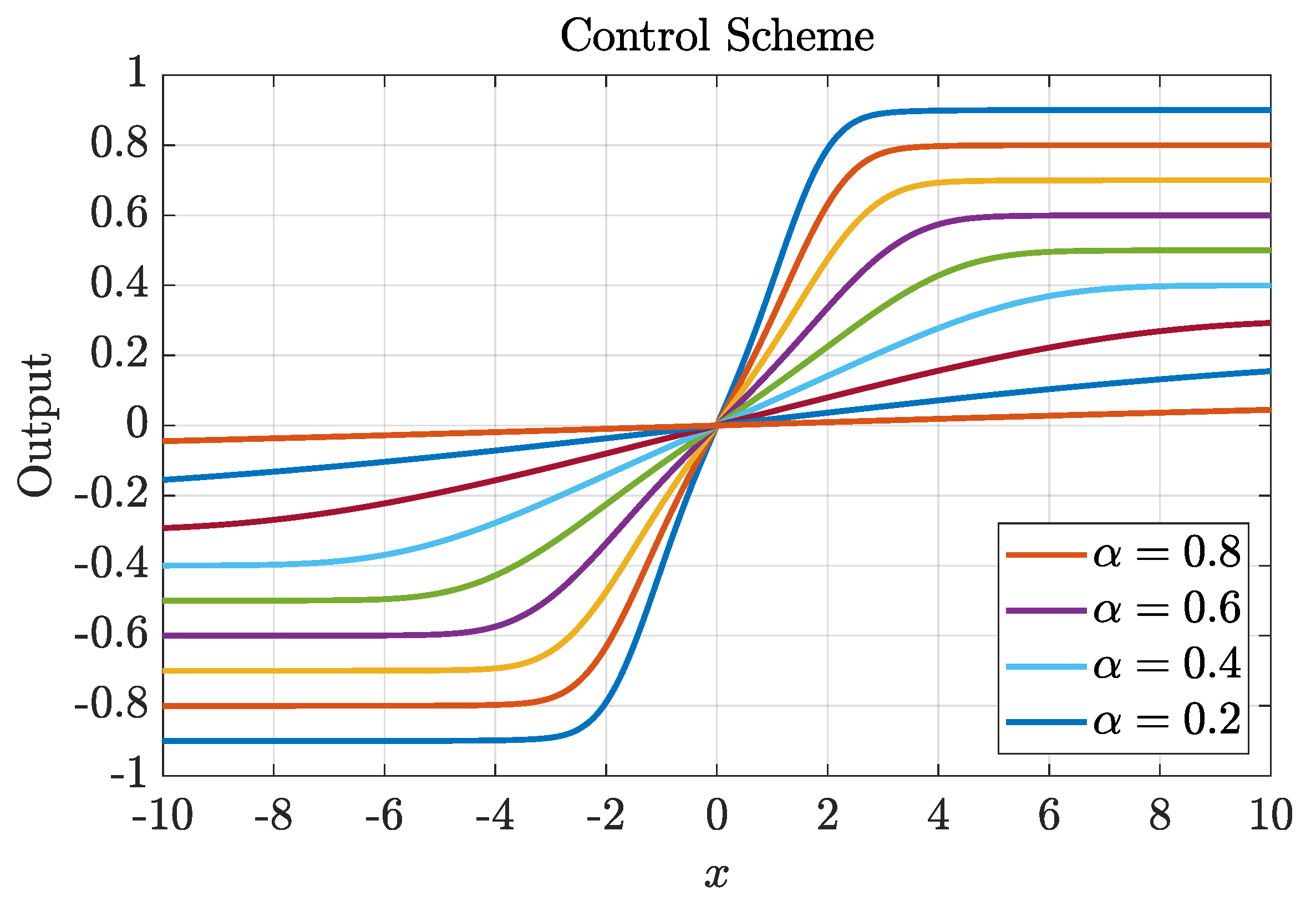
Figure 1 shows the qualitative behavior of the control structure composed of a suitable combination of hyperbolic functions. The basic structure for the three terms of the control algorithm (5) is ${\displaystyle \frac{\alpha (1-\alpha e^{-\alpha cosh\left(\alpha x\right)})sinh\left(\alpha x\right)}{cosh\left(\alpha x\right)+e^{-\alpha cosh\left(\alpha x\right)}}}$. This function is odd, located within the I and III quadrants, and its behavior is monotonically increasing, with saturation limits determined by $\alpha (1-\alpha e^{-\alpha cosh\left(\alpha x\right)})>0$; this function is also Lipschitz. The response varies for different values of the slope $\alpha$; when the value of $\alpha$ is close to 1, the slope tends to be vertical, causing a fast response in the function, while for $\alpha$ close to zero, the slope tends to be horizontal, resulting in slow responses. When the function is close to a neighborhood of the origin, its behavior is practically linear.

Each term of the proposed hyperbolic control law can be physically interpreted as follows: the component that depends on the position error acts as a nonlinear spring (Hooke’s law), where the proportional gain corresponds to the mechanical stiffness factor. The derivative control action is a nonlinear damper due to its hyperbolic characteristics, which injects artificial friction through joint velocity to obtain a greater dissipative effect, while the integral control action is related to a nonlinear capacitor that stores energy to be used primarily in the steady state in order to decrease the position error.

Another very important aspect, for the purposes of physical interpretation, is that the proposed hyperbolic function is obtained as the gradient of an artificial potential function $\mathcal{U}\left(\tilde{q}\right)$ as follows:

$$\mathcal{U}\left(\tilde{q}\right)=ln\left[cosh\left(\alpha \tilde{q}\right)+e^{-\alpha cosh\left(\alpha \tilde{q}\right)}\right]⟹{\displaystyle \frac{\partial }{\partial \tilde{q}}}\mathcal{U}\left(\tilde{q}\right)=\alpha {\displaystyle \frac{\left(1-\alpha e^{-\alpha cosh\left(\alpha \tilde{q}\right)}\right)sinh\left(\alpha \tilde{q}\right)}{cosh\left(\alpha \tilde{q}\right)+e^{-\alpha cosh\left(\alpha \tilde{q}\right)}}}$$

(15)

In other words, we are shaping the applied energy as if it were a nonlinear mechanical spring, whose stiffness corresponds to the proportional gain. This hyperbolic structure is replicated in the integral and derivative control actions.

3.2. Properties of the Hyperbolic Control Scheme

This subsection presents a useful mathematical property of the hyperbolic terms, which will be used in the stability analysis of the proposed control scheme.

Since $e>1⟹e^{cosh\left(\alpha x\right)}>1,\forall x\in \mathbb{R}$; then $e^{-\alpha cosh\left(\alpha x\right)}<1,\forall x\in \mathbb{R}$. Then, the following condition is satisfied: $0<1-\alpha e^{-\alpha cosh\left(\alpha x\right)}<1$.

On the other hand, the following conditions hold:

$$\begin{array}{cc}\hfill \alpha \left(1-\alpha e^{-\alpha cosh\left(\alpha x\right)}\right)x & < \alpha \left(1-\alpha e^{-\alpha cosh\left(\alpha x\right)}\right)sinh\left(\alpha x\right) < \alpha \left(cosh\left(\alpha x\right)+e^{-\alpha cosh\left(\alpha x\right)}\right)\left|x\right|\hfill \end{array}$$

(16)

$$\begin{array}{cc}\hfill \alpha {\displaystyle \frac{\left(1-\alpha e^{-\alpha cosh\left(\alpha x\right)}\right)}{cosh\left(\alpha x\right)+e^{-\alpha cosh\left(\alpha x\right)}}}x & < \alpha {\displaystyle \frac{\left(1-\alpha e^{-\alpha cosh\left(\alpha x\right)}\right)}{cosh\left(\alpha x\right)+e^{-\alpha cosh\left(\alpha x\right)}}}sinh\left(\alpha x\right) < \alpha \left|x\right|\hfill \end{array}$$

(17)

$$\begin{array}{cc}\hfill \alpha {\displaystyle \frac{\left(1-\alpha e^{-\alpha cosh\left(\alpha x\right)}\right)}{cosh\left(\alpha x\right)+e^{-\alpha cosh\left(\alpha x\right)}}}{\left|x\right|}^2 & < \alpha {\displaystyle \frac{\left(1-\alpha e^{-\alpha cosh\left(\alpha x\right)}\right)}{cosh\left(\alpha x\right)+e^{-\alpha cosh\left(\alpha x\right)}}}sinh\left(\alpha x\right)x < \alpha {\left|x\right|}^2\hfill \end{array}$$

(18)

There exist non-unique positive constants ${\psi }^l,{\psi }^u\in {\mathbb{R}}_{+}$ such that, taking ${\psi }^l\ll \left(1-\alpha e^{-\alpha cosh\left(\alpha x\right)}\right)$ as the lower bound and ${\psi }^u$ as the appropriately selected upper bound, the following inequality holds:

$$\alpha {\psi }^l{\displaystyle \frac{{\left|x\right|}^2}{cosh\left(\alpha x\right)+e^{-\alpha cosh\left(\alpha x\right)}}}\le {\displaystyle \frac{\alpha \left(1-\alpha e^{-\alpha cosh\left(\alpha x\right)}\right)}{cosh\left(\alpha x\right)+e^{-\alpha cosh\left(\alpha x\right)}}}sinh\left(\alpha x\right)x\le {\psi }^u\alpha {\left|x\right|}^2$$

(19)

Note that it is not strictly necessary to establish bounds for ${\psi }^l$ and ${\psi }^u$, since their numerical values are not required. However, we include them to complete the analysis by establishing an idea similar to the development in [32]. In fact, the lower ${\psi }^l$ and upper ${\psi }^u$ bounds are selected appropriately depending on the interval of x; in this context, those bounds are not unique.

Property 1.

There exist non-unique positive constants ${\psi }^u, {\psi }^l\in {\mathbb{R}}_{+}$ such that the following inequality holds for all $x\in \mathbb{R}$:

$$\alpha {\psi }^l{\displaystyle \frac{{\left|x\right|}^2}{cosh\left(\alpha x\right)+e^{-\alpha cosh\left(\alpha x\right)}}}\le {\displaystyle \frac{\alpha \left(1-\alpha e^{-\alpha cosh\left(\alpha x\right)}\right)}{cosh\left(\alpha x\right)+e^{-\alpha cosh\left(\alpha x\right)}}}sinh\left(\alpha x\right)x\le {\psi }^u\alpha {\left|x\right|}^2$$

(20)

Here, ${\psi }^l$ and ${\psi }^u$ denote lower and upper bounds, respectively.

A particular case of Property 1 is the following:

Property 2.

There exist a non-unique positive constant ${\psi }^u\in {\mathbb{R}}_{+}$ such that the following inequality holds for all $x,y\in \mathbb{R}$:

$${\displaystyle \frac{\alpha \left(1-\alpha e^{-\alpha cosh\left(\alpha x\right)}\right)}{cosh\left(\alpha x\right)+e^{-\alpha cosh\left(\alpha x\right)}}}sinh\left(\alpha x\right)y\le {\psi }^u\alpha \left|x\right|\left|y\right|$$

(21)

where ${\psi }^u$ denotes an upper bound.

4. Global Asymptotic Stability Analysis

This section presents the global asymptotic stability analysis of the two control schemes studied in this work: the classical linear PID controller and the proposed hyperbolic PID-type controller.

4.1. Linear PID Control

Proposition 1.

Given any initial condition ${\left[\tilde{q}\left(0\right), \overline{\epsilon }\left(0\right), \dot{q}\left(0\right)\right]}^T\in {\mathbb{R}}^3$, and selecting positive control gains $k_p, k_i, k_v$ for the linear PID control scheme (2), the state variables $\tilde{q}\left(t\right)$ (position error), $\overline{\epsilon }\left(t\right)$ (integral action), and $\dot{q}\left(t\right)$ (joint velocity) converge asymptotically to the equilibrium point of the closed-loop system (11). That is, the control objective is achieved as

$$\underset{t\to \infty }{lim}{\left[\tilde{q}\left(t\right), \overline{\epsilon }\left(t\right), \dot{q}\left(t\right)\right]}^T⟶{\left[0, 0, 0\right]}^T\in {\mathbb{R}}^3,\forall t\ge 0$$

(22)

Proof of Proposition 1.

To analyze the global asymptotic stability of the equilibrium point of system (11), consider the following Lyapunov function candidate. It is constructed as the sum of the pendulum’s kinetic energy, an artificial potential energy based on Hooke’s law, integral energy terms, and an auxiliary energy function composed of cross terms involving the position error $\tilde{q}$, the joint velocity $\dot{q}$, and the integral state $\overline{\epsilon }$:

$$\mathcal{V}(\tilde{q},\overline{\epsilon },\dot{q})={\displaystyle \frac{k_p}{2}}{\tilde{q}}^2+{\displaystyle \frac{k_i}{2}}{\overline{\epsilon }}^2+{\displaystyle \frac{\mathcal{I}}{2}}{\dot{q}}^2-{\displaystyle \frac{\mathcal{I}}{2}}{\omega }_0\tilde{q}\dot{q}-{\displaystyle \frac{\mathcal{I}}{2}}{\omega }_1\dot{q}\overline{\epsilon }-{\displaystyle \frac{k_p}{2}}{\omega }_2\tilde{q}\overline{\epsilon }$$

(23)

where ${\omega }_0,{\omega }_1,{\omega }_2$ are real positive scalar constants. These constants are introduced solely for the purpose of stability analysis and do not influence the control structure. Their exact numerical values are not required, as it is sufficient to prove the existence of values within an open interval where the Lyapunov function satisfies the required conditions.

To verify that the Lyapunov function candidate (23) is positive-definite, it can be rewritten in quadratic form as

$$\mathcal{V}(\tilde{q}, \overline{\epsilon }, \dot{q})={\displaystyle \frac{1}{2}}{\left[\begin{array}{c}\tilde{q}\\ \overline{\epsilon }\\ \dot{q}\end{array}\right]}^T\underset{P}{\underbrace{\left[\begin{array}{ccc}{k}_p& -{\displaystyle \frac{k_p}{2}}{\omega }_2& -{\displaystyle \frac{\mathcal{I}}{2}}{\omega }_0\\ -{\displaystyle \frac{k_p}{2}}{\omega }_2& k_i& -{\displaystyle \frac{\mathcal{I}}{2}}{\omega }_1\\ -{\displaystyle \frac{\mathcal{I}}{2}}{\omega }_0& -{\displaystyle \frac{\mathcal{I}}{2}}{\omega }_1& \mathcal{I}\end{array}\right]}}\left[\begin{array}{c}\tilde{q}\\ \overline{\epsilon }\\ \dot{q}\end{array}\right]$$

(24)

Applying Sylvester’s criterion, the matrix $P\in {\mathbb{R}}^{3\times 3}$ is positive definite if all its leading principal minors are positive. Given that $k_p>0$, $k_i>0$, and $\mathcal{I}>0$, this condition holds if the following inequalities are satisfied:

$$2\sqrt{{\displaystyle \frac{k_p}{\mathcal{I}}}}>{\omega }_0>0$$

(25)

$$2\sqrt{{\displaystyle \frac{k_i}{\mathcal{I}}}}>{\omega }_1>0$$

(26)

$$2\sqrt{{\displaystyle \frac{k_i}{k_p}}}>{\omega }_2>0$$

(27)

$$4{\displaystyle \frac{k_i}{\mathcal{I}}}>{\omega }_1^2+{\displaystyle \frac{1}{2}}{\omega }_0^2{\omega }_2^2+{\omega }_0{\omega }_1{\omega }_2>0$$

(28)

Therefore, under the conditions above, the function (23) is positive definite in the full state space ${\left[\tilde{q}\left(t\right), \overline{\epsilon }\left(t\right), \dot{q}\left(t\right)\right]}^T\in {\mathbb{R}}^3$.

The time derivative of the Lyapunov function candidate (23), evaluated along the trajectories of the closed-loop system (11), can be written as

$$\begin{array}{c}\dot{\mathcal{V}}(\tilde{q},\overline{\epsilon },\dot{q})=-{\displaystyle \frac{k_p}{2}}({\omega }_0+{\omega }_2){\tilde{q}}^2-\left[(k_v+b)-{\displaystyle \frac{\mathcal{I}}{2}}{\omega }_0\right]{\dot{q}}^2-{\displaystyle \frac{k_i{\omega }_1}{2}}{\overline{\epsilon }}^2+{\displaystyle \frac{1}{2}}\left[(k_v+b){\omega }_0-\mathcal{I}{\omega }_1\right]\tilde{q}\dot{q}\hfill \\ \hspace{1em}\hspace{1em}\hspace{1em}\hspace{1em}\hspace{1em}\hspace{1em}\hspace{1em}\hspace{1em}\hspace{1em}\hspace{1em}\hspace{1em}\hspace{1em}\hspace{1em}\hspace{1em}\hspace{1em}\hspace{1em}\hspace{1em}\hspace{1em}\hspace{1em}\hspace{1em}\hspace{1em}+\left[k_i-{\displaystyle \frac{k_i}{2}}{\omega }_0-{\displaystyle \frac{k_p}{2}}{\omega }_1\right]\tilde{q}\overline{\epsilon }+\left[k_i+{\displaystyle \frac{(k_v+b)}{2}}{\omega }_1+{\displaystyle \frac{k_p}{2}}{\omega }_2\right]\dot{q}\overline{\epsilon }\hfill \end{array}$$

(29)

The expression for $\dot{\mathcal{V}}(\tilde{q}, \overline{\epsilon }, \dot{q})$ in (29) can be equivalently rewritten in quadratic form as

$$\dot{\mathcal{V}}(\tilde{q}, \overline{\epsilon }, \dot{q})=-{\displaystyle \frac{1}{2}}{\left[\begin{array}{c}\tilde{q}\\ \overline{\epsilon }\\ \dot{q}\end{array}\right]}^T\underset{Q}{\underbrace{\left[\begin{array}{ccc}{k}_p({\omega }_0+{\omega }_2)& -k_i+{\displaystyle \frac{k_i}{2}}{\omega }_0+{\displaystyle \frac{k_p}{2}}{\omega }_1& -{\displaystyle \frac{(k_v+b)}{2}}{\omega }_0+{\displaystyle \frac{\mathcal{I}}{2}}{\omega }_1\\ -k_i+{\displaystyle \frac{k_i}{2}}{\omega }_0+{\displaystyle \frac{k_p}{2}}{\omega }_1& k_i{\omega }_1& -k_i-{\displaystyle \frac{(k_v+b)}{2}}{\omega }_1-{\displaystyle \frac{k_p}{2}}{\omega }_2\\ -{\displaystyle \frac{(k_v+b)}{2}}{\omega }_0+{\displaystyle \frac{\mathcal{I}}{2}}{\omega }_1& -k_i-{\displaystyle \frac{(k_v+b)}{2}}{\omega }_1-{\displaystyle \frac{k_p}{2}}{\omega }_2& 2(k_v+b)-\mathcal{I}{\omega }_0\end{array}\right]}}\left[\begin{array}{c}\tilde{q}\\ \overline{\epsilon }\\ \dot{q}\end{array}\right]$$

(30)

Applying Sylvester’s criterion once again, the matrix $Q\in {\mathbb{R}}^{3\times 3}$ is positive-definite if all of its principal minors and its determinant are positive. These conditions define existence intervals for the parameters ${\omega }_0, {\omega }_1, {\omega }_2$, as given below:

$${\displaystyle \frac{2\left(k_v+b\right)}{\mathcal{I}}}>{\omega }_0>0$$

(31)

$$1>{\omega }_0>0$$

(32)

$${\displaystyle \frac{2\left(k_v+b\right)}{\mathcal{I}}}>{\omega }_1>0$$

(33)

$${\omega }_0^2\left(1-{\displaystyle \frac{1}{4}}{\omega }_0\right)>{\omega }_1>0$$

(34)

$$2{\omega }_0>{\omega }_2>{\omega }_0>0$$

(35)

$${\displaystyle \frac{{\omega }_0{\omega }_2\left(2-{\omega }_0\right)}{8+2{\omega }_0+4{\omega }_2}}>{\omega }_1>0$$

(36)

$${\displaystyle \frac{64k_p{k}_i}{{\mathcal{I}}^2}}>{\displaystyle \frac{{\omega }_1\left(4{\omega }_1^2-4{\omega }_0{\omega }_1^2+{\omega }_0^2{\omega }_1^2+{\omega }_0^4+2{\omega }_0^3{\omega }_1\right)}{1+{\omega }_0+{\omega }_2}}>0$$

(37)

$$2{\displaystyle \frac{\left(k_v+b\right)}{\mathcal{I}}}>{\displaystyle \frac{\frac{5}{4}{\omega }_0^4+{\omega }_0^3{\omega }_2+{\omega }_1^2}{{\omega }_0^3+{\omega }_0^2{\omega }_2+{\omega }_0{\omega }_1}}>0$$

(38)

$$64{\displaystyle \frac{k_i\left(k_v+b\right)}{{\mathcal{I}}^2}}>16{\omega }_0{\omega }_1^2+4{\omega }_1^3+4{\omega }_0^2{\omega }_1+{\displaystyle \frac{{\omega }_0^4{\omega }_2^2}{{\omega }_1}}+4{\omega }_0^2{\omega }_1{\omega }_2+4{\omega }_0^3{\omega }_2>0$$

(39)

$$\begin{array}{c}256{\displaystyle \frac{k_i^2}{{\mathcal{I}}^3}}\left[\mathcal{I}+(k_v+b)\right]>16{\displaystyle \frac{{\omega }_1^4}{{\omega }_0}}\left({\omega }_0^2-{\omega }_1-{\displaystyle \frac{1}{4}}{\omega }_0^3\right)+16{\omega }_0{\omega }_1^3\left({\displaystyle \frac{k_v+b}{\mathcal{I}}}-{\displaystyle \frac{1}{2}}{\omega }_1\right)+16{\omega }_0{\omega }_1^3\left({\omega }_0-{\displaystyle \frac{1}{2}}{\omega }_2\right)\hfill \\ \hspace{1em}\hspace{1em}\hspace{1em}\hspace{1em}\hspace{1em}\hspace{1em}\hspace{1em}+8{\omega }_0^2{\omega }_1^2\left({\displaystyle \frac{1}{2}}{\omega }_0{\omega }_2-2{\omega }_1-{\displaystyle \frac{1}{2}}{\omega }_0{\omega }_1-{\omega }_1{\omega }_2-{\displaystyle \frac{1}{4}}{\omega }_0^2{\omega }_2\right)+8{\omega }_0^3{\omega }_1^3+16{\displaystyle \frac{{\omega }_1^5}{{\omega }_0}}+8{\omega }_1^5+8{\omega }_0{\omega }_1^4+4{\omega }_0^2{\omega }_1^4+4{\omega }_0^4{\omega }_1^2\hfill \\ \hspace{1em}\hspace{1em}\hspace{1em}\hspace{1em}\hspace{1em}\hspace{1em}\hspace{1em}\hspace{1em}\hspace{1em}+4{\omega }_0^3{\omega }_1^2{\omega }_2+4{\omega }_0^4{\omega }_1^2{\omega }_2+4{\omega }_0^3{\omega }_1^2{\omega }_2^2+20{\omega }_0^2{\omega }_1^3{\omega }_2+32{\omega }_1^2\left(2{\displaystyle \frac{k_i}{\mathcal{I}}}-{\displaystyle \frac{1}{2}}{\omega }_1^2\right)+2{\omega }_0^5{\omega }_1{\omega }_2+{\omega }_0^6{\omega }_2^2+4{\omega }_0^4{\omega }_1{\omega }_2^2+{\omega }_0^5{\omega }_2^3>0\hfill \end{array}$$

(40)

Thus, the time derivative $\dot{\mathcal{V}}(\tilde{q}, \overline{\epsilon }, \dot{q})$, defined in (30), is a negative-definite function, and the proposed Lyapunov function $\mathcal{V}(\tilde{q}, \overline{\epsilon }, \dot{q})$, given in (23), is a positive definite function. Therefore, $\mathcal{V}$ is a strict Lyapunov function. Consequently, there exist parameters ${\omega }_0, {\omega }_1, {\omega }_2$ satisfying the conditions (25)–(28) and (31)–(40). According to Lyapunov’s direct method, this guarantees the asymptotic stability of the equilibrium point ${\left[\tilde{q}, \overline{\epsilon }, \dot{q}\right]}^T={\left[0, 0, 0\right]}^T\in {\mathbb{R}}^3$ for the closed-loop system (11). This completes the proof. □

4.2. Hyperbolic PID-Type Control

Proposition 2.

Given any initial condition ${\left[\tilde{q}\left(0\right), {\overline{\epsilon }}_h\left(0\right), \dot{q}\left(0\right)\right]}^T\in {\mathbb{R}}^3$, and selecting positive control gains $k_p, k_i, k_v$ for the hyperbolic PID-type control scheme (5), the state variables $\tilde{q}\left(t\right)$ (position error), ${\overline{\epsilon }}_h\left(t\right)$ (integral action), and $\dot{q}\left(t\right)$ (joint velocity) converge asymptotically to the equilibrium point of the closed-loop system (13). That is, the control objective is achieved as

$$\underset{t\to \infty }{lim}{\left[\tilde{q}\left(t\right), {\overline{\epsilon }}_h\left(t\right), \dot{q}\left(t\right)\right]}^T⟶{\left[0, 0, 0\right]}^T\in {\mathbb{R}}^3,\forall t\ge 0$$

(41)

Proof of Proposition 2.

To analyze the global asymptotic stability of the equilibrium point of system (13), the strict Lyapunov function previously defined in (30) is reformulated to accommodate the structure of the hyperbolic PID-type control law (5). The proposed Lyapunov function consists of the sum of the pendulum’s kinetic energy, an artificial potential energy based on Hooke’s law, integral energy terms, and an auxiliary energy function composed of cross terms involving the position error $\tilde{q}$, the joint velocity $\dot{q}$, and the integral state ${\overline{\epsilon }}_h$. Additionally, an artificial potential energy term derived from the hyperbolic control structure is included:

$${\mathcal{V}}_h(\tilde{q}, {\overline{\epsilon }}_h, \dot{q})={\displaystyle \frac{k_p}{2}}{\tilde{q}}^2+{\displaystyle \frac{k_i}{2}}{\overline{\epsilon }}_h^2+{\displaystyle \frac{\mathcal{I}}{2}}{\dot{q}}^2-{\displaystyle \frac{\mathcal{I}}{2}}{\varphi }_0\tilde{q}\dot{q}-{\displaystyle \frac{\mathcal{I}}{2}}{\varphi }_1\dot{q}{\overline{\epsilon }}_h-{\displaystyle \frac{k_i}{2}}{\varphi }_2\tilde{q}{\overline{\epsilon }}_h+k_p\left(ln\left[cosh\left(\alpha \tilde{q}\right)+e^{-\alpha cosh\left(\alpha \tilde{q}\right)}\right]-ln\left[1+e^{-\alpha }\right]\right)$$

(42)

where ${\varphi }_0, {\varphi }_1, {\varphi }_2$ are real positive scalar constants. As with the linear PID case, it is important to emphasize that these scalars are introduced solely for the purpose of the stability analysis. Therefore, it is not necessary to determine their numerical values, as they do not form part of the control law itself. It suffices to demonstrate that such parameters exist within some open interval, whether defined through linear or nonlinear combinations among themselves.

The Lyapunov function candidate defined in (42) can be rewritten in a more compact form as follows:

$${\mathcal{V}}_h(\tilde{q}, {\overline{\epsilon }}_h, \dot{q})={\displaystyle \frac{1}{2}}{\left[\begin{array}{c}\tilde{q}\\ {\overline{\epsilon }}_h\\ \dot{q}\end{array}\right]}^T\underset{P_h}{\underbrace{\left[\begin{array}{ccc}{k}_p& -{\displaystyle \frac{k_i}{2}}{\varphi }_2& -{\displaystyle \frac{\mathcal{I}}{2}}{\varphi }_0\\ -{\displaystyle \frac{k_i}{2}}{\varphi }_2& k_i& -{\displaystyle \frac{\mathcal{I}}{2}}{\varphi }_1\\ -{\displaystyle \frac{\mathcal{I}}{2}}{\varphi }_0& -{\displaystyle \frac{\mathcal{I}}{2}}{\varphi }_1& \mathcal{I}\end{array}\right]}}\left[\begin{array}{c}\tilde{q}\\ {\overline{\epsilon }}_h\\ \dot{q}\end{array}\right]+k_p\left(ln\left[cosh\left(\alpha \tilde{q}\right)+e^{-\alpha cosh\left(\alpha \tilde{q}\right)}\right]-ln\left[1+e^{-\alpha }\right]\right)$$

(43)

The first part of the equation, $P_h\in {\mathbb{R}}^{3\times 3}$, is a positive-definite matrix equivalent to the matrix P from the linear PID case, and the second term is a positive definite function on its own. This implies that, for the function (43) to qualify as a positive-definite Lyapunov candidate in the full state ${\left[\tilde{q}\left(t\right), {\overline{\epsilon }}_h\left(t\right), \dot{q}\left(t\right)\right]}^T$, conditions (25)–(28) must be satisfied for the parameters ${\varphi }_0, {\varphi }_1, {\varphi }_2$; that is

$$2\sqrt{{\displaystyle \frac{k_p}{\mathcal{I}}}}>{\varphi }_0>0$$

(44)

$$2\sqrt{{\displaystyle \frac{k_i}{\mathcal{I}}}}>{\varphi }_1>0$$

(45)

$$2\sqrt{{\displaystyle \frac{k_i}{k_p}}}>{\varphi }_2>0$$

(46)

$$4{\displaystyle \frac{k_i}{\mathcal{I}}}>{\varphi }_1^2+{\displaystyle \frac{1}{2}}{\varphi }_0^2{\varphi }_2^2+{\varphi }_0{\varphi }_1{\varphi }_2>0$$

(47)

Therefore, under the conditions above, the function (42) is positive-definite in the full state space ${\left[\tilde{q}\left(t\right), {\overline{\epsilon }}_h\left(t\right), \dot{q}\left(t\right)\right]}^T\in {\mathbb{R}}^3$.

The time derivative of the Lyapunov function candidate (42) along the trajectories of the closed-loop Equation (13) is obtained as follows:

$$\begin{array}{c}{\dot{\mathcal{V}}}_h(\tilde{q},{\overline{\epsilon }}_h,\dot{q})=-b{\dot{q}}^2-k_p\tilde{q}\dot{q}-{\displaystyle \frac{k_i{\varphi }_0}{2}}{\overline{\epsilon }}_h\tilde{q}-{\displaystyle \frac{k_i{\varphi }_1}{2}}{\overline{\epsilon }}_h^2+k_i\dot{q}{\overline{\epsilon }}_h+{\displaystyle \frac{\mathcal{I}{\varphi }_0}{2}}{\dot{q}}^2+{\displaystyle \frac{b{\varphi }_0}{2}}\dot{q}\tilde{q}+{\displaystyle \frac{b{\varphi }_1}{2}}\dot{q}{\overline{\epsilon }}_h+{\displaystyle \frac{k_i{\varphi }_2}{2}}\dot{q}{\overline{\epsilon }}_h\hfill \\ \hspace{1em}\hspace{1em}\hspace{1em}\hspace{1em} -{\displaystyle \frac{k_v\beta \left(1-\beta e^{-\beta cosh\left(\beta \dot{q}\right)}\right)}{cosh\left(\beta \dot{q}\right)+e^{-\beta cosh\left(\beta \dot{q}\right)}}}sinh\left(\beta \dot{q}\right)\dot{q}-{\displaystyle \frac{k_p{\varphi }_0}{2}}{\displaystyle \frac{\alpha \left(1-\alpha e^{-\alpha cosh\left(\alpha \tilde{q}\right)}\right)}{cosh\left(\alpha \tilde{q}\right)+e^{-\alpha cosh\left(\alpha \tilde{q}\right)}}}sinh\left(\alpha \tilde{q}\right)\tilde{q}-{\displaystyle \frac{k_p{\varphi }_1}{2}}{\displaystyle \frac{\alpha \left(1-\alpha e^{-\alpha cosh\left(\alpha \tilde{q}\right)}\right)}{cosh\left(\alpha \tilde{q}\right)+e^{-\alpha cosh\left(\alpha \tilde{q}\right)}}}sinh\left(\alpha \tilde{q}\right){\overline{\epsilon }}_h\hfill \\ \hspace{1em}\hspace{1em}\hspace{1em}\hspace{1em} -{\displaystyle \frac{\mathcal{I}{\varphi }_1}{2}}{\displaystyle \frac{\gamma \left(1-\gamma e^{-\gamma cosh\left(\gamma \tilde{q}\right)}\right)}{cosh\left(\gamma \tilde{q}\right)+e^{-\gamma cosh\left(\gamma \tilde{q}\right)}}}sinh\left(\gamma \tilde{q}\right)\dot{q}-{\displaystyle \frac{k_i{\varphi }_2}{2}}{\displaystyle \frac{\gamma \left(1-\gamma e^{-\gamma cosh\left(\gamma \tilde{q}\right)}\right)}{cosh\left(\gamma \tilde{q}\right)+e^{-\gamma cosh\left(\gamma \tilde{q}\right)}}}sinh\left(\gamma \tilde{q}\right)\tilde{q}+k_i{\overline{\epsilon }}_h{\displaystyle \frac{\gamma \left(1-\gamma e^{-\gamma cosh\left(\gamma \tilde{q}\right)}\right)}{cosh\left(\gamma \tilde{q}\right)+e^{-\gamma cosh\left(\gamma \tilde{q}\right)}}}sinh\left(\gamma \tilde{q}\right)\hfill \\ \hspace{1em}\hspace{1em}\hspace{1em}\hspace{1em}\hspace{1em}\hspace{1em}\hspace{1em}\hspace{1em}\hspace{1em}\hspace{1em}\hspace{1em}\hspace{1em}\hspace{1em}\hspace{1em}\hspace{1em}\hspace{1em}\hspace{1em}\hspace{1em}\hspace{1em}\hspace{1em}\hspace{1em}\hspace{1em} +{\displaystyle \frac{k_v{\varphi }_0}{2}}{\displaystyle \frac{\beta \left(1-\beta e^{-\beta cosh\left(\beta \dot{q}\right)}\right)}{cosh\left(\beta \dot{q}\right)+e^{-\beta cosh\left(\beta \dot{q}\right)}}}sinh\left(\beta \dot{q}\right)\tilde{q}+{\displaystyle \frac{k_v{\varphi }_1}{2}}{\displaystyle \frac{\beta \left(1-\beta e^{-\beta cosh\left(\beta \dot{q}\right)}\right)}{cosh\left(\beta \dot{q}\right)+e^{-\beta cosh\left(\beta \dot{q}\right)}}}sinh\left(\beta \dot{q}\right){\overline{\epsilon }}_h\hfill \end{array}$$

(48)

Instead of analyzing the negative-definiteness of function (48) directly, a more convenient strictly greater function will be analyzed, making so that if this new function is negative-definite, function (48) must also be negatively defined. To obtain this function, we proceed to derive upper bounds for each term on the right-hand side of function (48) using the absolute value of the state variables. These bounds are specially selected to ease the application of Sylvester’s criterion later on. For the first nine terms, the bounds can be obtained directly, for example, through $-b{\dot{q}}^2\le -b{\left|\dot{q}\right|}^2$, $-k_p\tilde{q}\dot{q}\le k_p|\tilde{q}||\dot{q}|$ or $-{\displaystyle \frac{k_i{\varphi }_0}{2}}{\overline{\epsilon }}_h\tilde{q}\le k_i{\varphi }_0|{\overline{\epsilon }}_h||\tilde{q}|$. The last eight terms follow directly from the properties (1)–(2), such as

$$-{\displaystyle \frac{k_v\beta (1-\beta e^{-\beta cosh\left(\beta \dot{q}\right)})}{cosh\left(\beta \dot{q}\right)+e^{-\beta cosh\left(\beta \dot{q}\right)}}}sinh\left(\beta \dot{q}\right)\dot{q}\le -{\displaystyle \frac{1}{2}}{\displaystyle \frac{k_v\beta {\psi }^l{\left|\dot{q}\right|}^2}{cosh\left(\beta \dot{q}\right)+e^{-\beta cosh\left(\beta \dot{q}\right)}}}$$

(49)

or

$$-{\displaystyle \frac{k_p{\varphi }_1}{2}}{\displaystyle \frac{\alpha (1-\alpha e^{-\alpha cosh\left(\alpha \tilde{q}\right)})}{cosh\left(\alpha \tilde{q}\right)+e^{-\alpha cosh\left(\alpha \tilde{q}\right)}}}sinh\left(\alpha \tilde{q}\right){\overline{\epsilon }}_h\le k_p\alpha {\varphi }_1{\psi }^u|\tilde{q}\left|\right|{\overline{\epsilon }}_h|$$

(50)

After performing algebraic grouping and term reduction, Equation (48) can be rewritten as

$$\begin{array}{c}{\dot{\mathcal{V}}}_h(\tilde{q},{\overline{\epsilon }}_h,\dot{q})\le -{\displaystyle \frac{1}{2}}\left[{\displaystyle \frac{k_p\alpha {\varphi }_0{\psi }^l}{cosh\left(\alpha \tilde{q}\right)+e^{-\alpha cosh\left(\alpha \tilde{q}\right)}}}+{\displaystyle \frac{k_i\gamma {\varphi }_2{\psi }^l}{cosh\left(\gamma \tilde{q}\right)+e^{-\gamma cosh\left(\gamma \tilde{q}\right)}}}\right]|\tilde{q}{|}^2-{\displaystyle \frac{1}{2}}{k}_i{\varphi }_1{|{\overline{\epsilon }}_h|}^2\hfill \\ \hspace{1em}\hspace{1em}\hspace{1em}\hspace{1em}\hspace{1em}-{\displaystyle \frac{1}{2}}\left[{\displaystyle \frac{k_v\beta {\psi }^l}{cosh\left(\beta \dot{q}\right)+e^{-\beta cosh\left(\beta \dot{q}\right)}}}+2b-\mathcal{I}{\varphi }_0\right]|\dot{q}{|}^2+\left[k_p+(k_v\beta {\psi }^u+b){\varphi }_0+\mathcal{I}\gamma {\varphi }_1{\psi }^u\right]|\tilde{q}||\dot{q}|\hfill \\ \hspace{1em}\hspace{1em}\hspace{1em}\hspace{1em}\hspace{1em}\hspace{1em}\hspace{1em}\hspace{1em}\hspace{1em}\hspace{1em}\hspace{1em}\hspace{1em}\hspace{1em}\hspace{1em}\hspace{1em} +\left[k_i{\varphi }_0+k_p\alpha {\varphi }_1{\psi }^u+k_i\gamma {\psi }^u\right]|\tilde{q}||{\overline{\epsilon }}_h|+\left[k_i+(k_v\beta {\psi }^u+b){\varphi }_1+k_i{\varphi }_2\right]|\dot{q}||{\overline{\epsilon }}_h|\hfill \end{array}$$

(51)

To facilitate the analysis, inequality (51) can be reformulated as

$${\dot{\mathcal{V}}}_h(\tilde{q},{\overline{\epsilon }}_h,\dot{q})\le -{\displaystyle \frac{1}{2}}{\left[\begin{array}{c}\tilde{q}\\ {\overline{\epsilon }}_h\\ \dot{q}\end{array}\right]}^T\underset{Q_h}{\underbrace{\left[\begin{array}{ccc}{\displaystyle \frac{k_p\alpha {\varphi }_0{\psi }^l}{cosh\left(\alpha \tilde{q}\right)+e^{-\alpha cosh\left(\alpha tildeq\right)}}}+{\displaystyle \frac{k_i\gamma {\varphi }_2{\psi }^l}{cosh\left(\gamma \tilde{q}\right)+e^{-\gamma cosh\left(\gamma \tilde{q}\right)}}}& -\left[k_i{\varphi }_0+k_p\alpha {\varphi }_1{\psi }^u+k_i\gamma {\psi }^u\right]& -\left[k_p+(k_v\beta {\psi }^u+b){\varphi }_0+\mathcal{I}\gamma {\varphi }_1{\psi }^u\right]\\ -\left[k_i{\varphi }_0+k_p\alpha {\varphi }_1{\psi }^u+k_i\gamma {\psi }^u\right]& k_i{\varphi }_1& -\left[k_i+(k_v\beta {\psi }^u+b){\varphi }_1+k_i{\varphi }_2\right]\\ -\left[k_p+(k_v\beta {\psi }^u+b){\varphi }_0+\mathcal{I}\gamma {\varphi }_1{\psi }^u\right]& -\left[k_i+(k_v\beta {\psi }^u+b){\varphi }_1+k_i{\varphi }_2\right]& {\displaystyle \frac{k_v\beta {\psi }^l}{cosh\left(\beta \dot{q}\right)+e^{-\beta cosh\left(\beta \dot{q}\right)}}}+2b-\mathcal{I}{\varphi }_0\end{array}\right]}}\left[\begin{array}{c}\tilde{q}\\ {\overline{\epsilon }}_h\\ \dot{q}\end{array}\right]$$

(52)

As in the linear PID case, applying Sylvester’s criterion to the matrix $Q_h$ yields the conditions on the parameters ${\varphi }_0,{\varphi }_1,{\varphi }_2$ required to ensure that the matrix is positive-definite:

$${\displaystyle \frac{1}{\mathcal{I}}}\left({\displaystyle \frac{k_v\beta {\psi }^l}{cosh\left(\beta \dot{q}\right)+e^{-\beta cosh\left(\beta \dot{q}\right)}}}+2b\right)>{\varphi }_0>0$$

(53)

$${\displaystyle \frac{1}{\left(cosh\left(\gamma \tilde{q}\right)+e^{-\gamma cosh\left(\gamma \tilde{q}\right)}\right)\left(cosh\left(\alpha \tilde{q}\right)+e^{-\alpha cosh\left(\alpha \tilde{q}\right)}\right)}}>{\displaystyle \frac{{\left({\varphi }_0{\varphi }_1+\alpha {\varphi }_0^2{\psi }^u+\gamma {\varphi }_1{\psi }^u\right)}^2}{\alpha {\varphi }_0^3{\varphi }_1{\psi }^l\left(cosh\left(\gamma \tilde{q}\right)+e^{-\gamma cosh\left(\gamma \tilde{q}\right)}\right)+\gamma {\varphi }_1^3{\varphi }_2{\psi }^l\left(cosh\left(\alpha \tilde{q}\right)+e^{-\alpha cosh\left(\alpha \tilde{q}\right)}\right)}}>0$$

(54)

$${\displaystyle \frac{1}{\mathcal{I}}}{\displaystyle \frac{k_v\beta {\psi }^l}{cosh\left(\beta \dot{q}\right)+e^{-\beta cosh\left(\beta \dot{q}\right)}}}+{\displaystyle \frac{2b}{\mathcal{I}}}>{\varphi }_0+{\displaystyle \frac{\left(cosh\left(\gamma \tilde{q}\right)+e^{-\gamma cosh\left(\gamma \tilde{q}\right)}\right)\left(cosh\left(\alpha \tilde{q}\right)+e^{-\alpha cosh\left(\alpha \tilde{q}\right)}\right){\left(\frac{1}{2}{\varphi }_0^2+2\gamma {\varphi }_1{\psi }^u\right)}^2}{\alpha {\varphi }_0^3{\psi }^l\left(cosh\left(\gamma \tilde{q}\right)+e^{-\gamma cosh\left(\gamma \tilde{q}\right)}\right)+\gamma {\varphi }_1^2{\varphi }_2{\psi }^l\left(cosh\left(\alpha \tilde{q}\right)+e^{-\alpha cosh\left(\alpha \tilde{q}\right)}\right)}}>0$$

(55)

$${\displaystyle \frac{4}{\mathcal{I}}}{\displaystyle \frac{k_v\beta {\psi }^l}{cosh\left(\beta \dot{q}\right)+e^{-\beta cosh\left(\beta \dot{q}\right)}}}>4{\varphi }_0+{\varphi }_1{(1+{\varphi }_2)}^2>0$$

(56)

$$\begin{array}{c}{\displaystyle \frac{4\left(\frac{k_v\beta {\psi }^l}{cosh\left(\beta \dot{q}\right)+e^{-\beta cosh\left(\beta \dot{q}\right)}}+b\right)}{\mathcal{I}\left(cosh\left(\gamma \tilde{q}\right)+e^{-\gamma cosh\left(\gamma \tilde{q}\right)}\right)\left(cosh\left(\alpha \tilde{q}\right)+e^{-\alpha cosh\left(\alpha \tilde{q}\right)}\right)}}>{\displaystyle \frac{{\varphi }_1{(1+{\varphi }_2)}^2+4{\varphi }_0}{\left(cosh\left(\gamma \tilde{q}\right)+e^{-\gamma cosh\left(\gamma \tilde{q}\right)}\right)\left(cosh\left(\alpha \tilde{q}\right)+e^{-\alpha cosh\left(\alpha \tilde{q}\right)}\right)}}\hfill \\ \hspace{1em}\hspace{1em}\hspace{1em}\hspace{1em}\hspace{1em}\hspace{1em}\hspace{1em}\hspace{1em}\hspace{1em}\hspace{1em}\hspace{1em}\hspace{1em}\hspace{1em}\hspace{1em}\hspace{1em} +{\displaystyle \frac{1}{\alpha {\varphi }_0^3{\psi }^l\left(cosh\left(\gamma \tilde{q}\right)+e^{-\gamma cosh\left(\gamma \tilde{q}\right)}\right)+\gamma {\varphi }_1^2{\varphi }_2{\psi }^l\left(cosh\left(\alpha \tilde{q}\right)+e^{-\alpha cosh\left(\alpha \tilde{q}\right)}\right)}}\hfill \\ \hspace{1em}\hspace{1em}\hspace{1em}\hspace{1em}\hspace{1em}\hspace{1em}\hspace{1em}\hspace{1em}\hspace{1em}[4\left({\displaystyle \frac{1}{\mathcal{I}}}\left({\displaystyle \frac{k_v\beta {\psi }^l}{cosh\left(\beta \dot{q}\right)+e^{-\beta cosh\left(\beta \dot{q}\right)}}}+b\right)-{\varphi }_0\right){\left(\gamma \sqrt{{\varphi }_1}{\psi }^u+{\varphi }_0\sqrt{{\varphi }_1}+\alpha {\displaystyle \frac{{\varphi }_0^2}{\sqrt{{\varphi }_1}}}{\psi }^u\right)}^2+2\gamma {\varphi }_0^2{\varphi }_1{\psi }^u(5+{\varphi }_2)\hfill \\ \hspace{1em}\hspace{1em}\hspace{1em}\hspace{1em}\hspace{1em}\hspace{1em}\hspace{1em}\hspace{1em}\hspace{1em}\hspace{1em}\hspace{1em}\hspace{1em}\hspace{1em}\hspace{1em}\hspace{1em}\hspace{1em}\hspace{1em}\hspace{1em} +2{\varphi }_0^3{\varphi }_1({\varphi }_1+{\varphi }_2)+{\varphi }_0^4+8{\gamma }^2{\varphi }_1^2{{\psi }^u}^2(3+{\varphi }_2)+2{\varphi }_0{\psi }^u\left(\alpha {\varphi }_0^3+4\gamma {\varphi }_1(\alpha {\varphi }_0{\psi }^u+{\varphi }_1)\right)(1+{\varphi }_2)]>0\hfill \end{array}$$

(57)

Thus, ${\dot{\mathcal{V}}}_h(\tilde{q},{\overline{\epsilon }}_h,\dot{q})<0$, as defined in (48), is a negative-definite function. Since the proposed Lyapunov function ${\mathcal{V}}_h(\tilde{q},{\overline{\epsilon }}_h,\dot{q})>0$, defined in (42), is positive-definite, it follows that ${\mathcal{V}}_h$ is a strict Lyapunov function.

Consequently, the existence of parameters ${\varphi }_0,{\varphi }_1,{\varphi }_2$ satisfying the conditions in (44)–(47) and (53)–(57) is guaranteed. Therefore, by Lyapunov’s direct method, the equilibrium point ${\left[\tilde{q}, {\overline{\epsilon }}_h, \dot{q}\right]}^T={\left[0, 0, 0\right]}^T\in {\mathbb{R}}^3$ of the closed-loop system (13) is asymptotically stable. This completes the proof. □

4.3. Remark on Feasibility of the Auxiliary Conditions

Although the explicit inequalities (31)–(40) and (53)–(57) appear lengthy, their feasibility is not restrictive. The auxiliary parameters ${\omega }_i$ and ${\varphi }_i$ introduced in the Lyapunov functions are used exclusively for Lyapunov analysis purposes and do not form part of the control law. The inequalities derived above arise from the application of Sylvester’s criterion to guarantee the positive definiteness of the Lyapunov function and the negative definiteness of its derivative. Although these conditions appear algebraically involved, their structure mainly imposes upper bounds and ordering relations among the auxiliary parameters. Since all inequalities are continuous with respect to these variables and the origin belongs to their admissible region, there always exists a non-empty open set of sufficiently small values that satisfies all conditions simultaneously. Therefore, these requirements should be interpreted as theoretical feasibility conditions ensuring the existence of a strict Lyapunov function rather than practical tuning rules.

5. Experimental Results

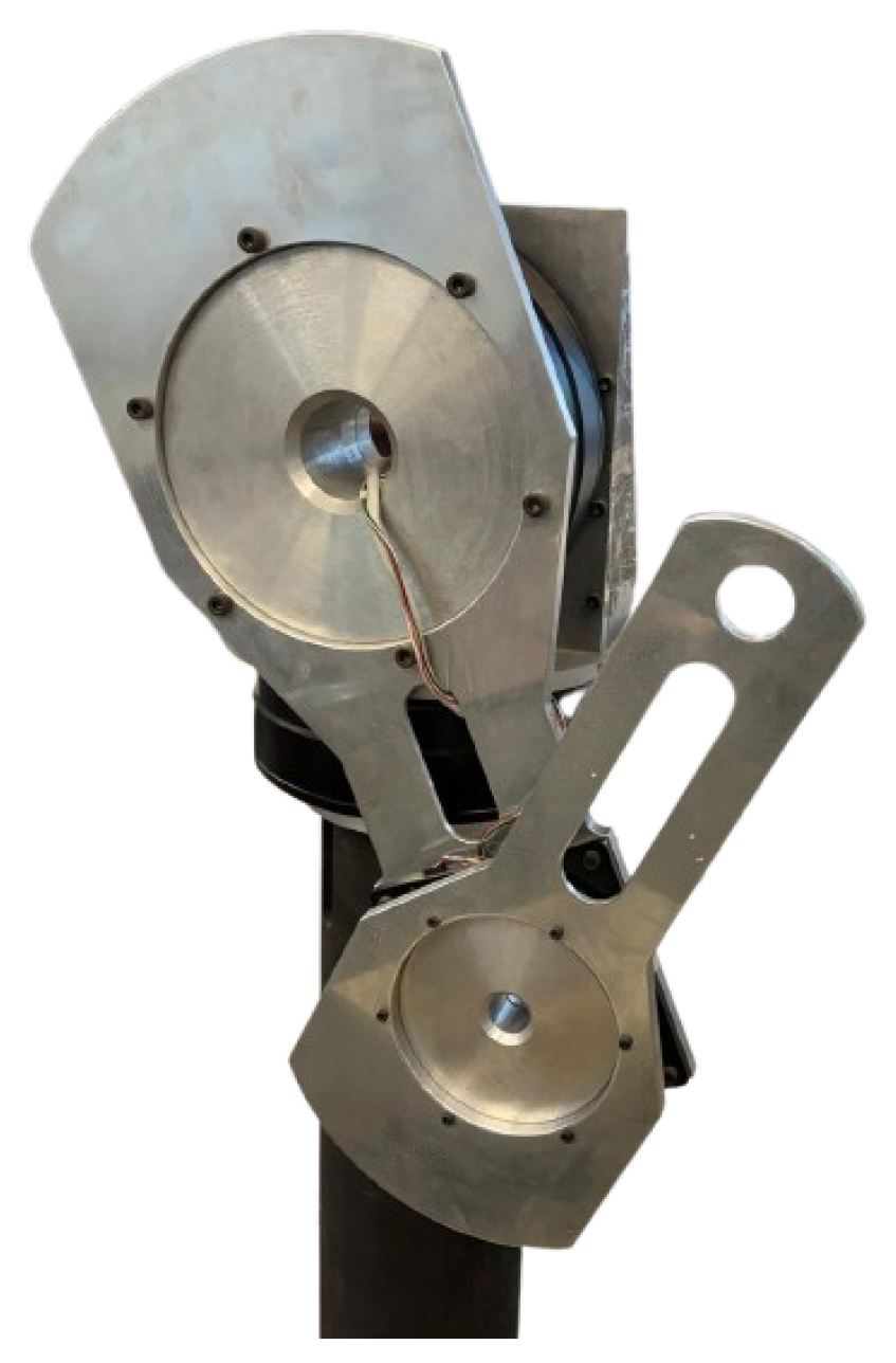
This section describes the experimental setup and presents the time-real results for the two evaluated control schemes: linear PID and proposed hyperbolic PID-Type algorithms. The experimental system consists of a direct-drive pendulum, which forms part of a 3-degree-of-freedom (3-DOF) manipulator robot. The pendulum is located at the third joint (the elbow joint), as illustrated in Figure 2; the base and shoulder joints were controlled at zero degrees using position algorithms with hyperbolic tangent structure [33].

The pendulum link is constructed from 6061 aluminum and is actuated by a brushless direct-drive servomotor (from Parker Compumotor), which drives the joint without gear reduction. Direct-drive actuators offer several advantages: they are free from backlash, exhibit significantly lower friction compared to gear-driven actuators, and when operated in torque mode, it accepts an analog voltage as a reference of torque signal (12 bits), then it provides an ideal source of applied torque. The specific servomotor model used in the experimental setup is listed in

Table 1. Servo actuator of the direct-drive pendulum.

Link	Model	Torque [Nm]	Encoder [p/rev]
Elbow	DM1004C	4	2,621,440

.

The pendulum electronic interface consists of an embedded system composed by MKR Vidor 4000 from Arduino—which includes on the same board a Cortex-M0 32-bit SAMD21 microprocessor (48 Mhz, 256 KB flash and 32 KB SRAM) of the MKR-family—and a FPGA chip (Intel Cyclone 10CL016).

Position information $q\left(t_k\right)$ is obtained from an incremental encoder of the servomotor, which is read using an incremental counter programmed at FPGA with VHDL language through Quartus programming environment; while the velocity signal $\dot{q}\left(t_k\right)$ is computed using a standard backward difference algorithm (Euler method) applied to the position measurements: $\dot{q}\left(t_k\right)\approx {\displaystyle \frac{q\left(t_k\right)-q\left(t_{k-1}\right)}{h}}$. The integral states were computed using Euler’s numerical integration technique; for the classical PID: $\epsilon \left(t_k\right)=\epsilon \left(t_{k-1}\right)+h\tilde{q}\left(t_k\right)$, and the hyperbolic PID: ${\epsilon }_h\left(t_k\right)={\epsilon }_h\left(t_{k-1}\right)+h{\displaystyle \frac{\gamma \left(1-\gamma e^{-\gamma cosh\left(\gamma \tilde{q}\left(t_k\right)\right)}\right)}{cosh\left(\gamma \tilde{q}\left(t_k\right)\right)+e^{-\gamma cosh\left(\gamma \tilde{q}\left(t_k\right)\right)}}}sinh\left(\gamma \tilde{q}\left(t_k\right)\right)$. The numerical methods and control algorithms, with their parameters and gains implemented on the microprocessor with the C programming language and executed in real time with a sampling period of $h=2.5$ ms.

The experimental results presented in this Section are the usual ones for the case of regulation (15 s per experiment): they consist of moving the pendulum from the initial condition (home-position: $\tilde{q}\left(0\right)=q_d,{\dot{q}}_1\left(0\right)=0$, and $\overline{\epsilon }\left(0\right)={\overline{\epsilon }}_h\left(0\right)=0$) towards a desired reference $q_d$ or set-point, constant at time. Three different references have been considered: $q_{d1}={\displaystyle \frac{\pi }{2}}$, $q_{d2}={\displaystyle \frac{\pi }{4}}$, and $q_{d3}=3{\displaystyle \frac{\pi }{4}}$. One reference for each experiment for both evaluated control schemes: the linear PID scheme (2) and the proposed hyperbolic PID-type control (5). With respect to the pendulum dynamics, only the gravitational torque $g_{T\left(q\right)}=0.4562sin\left(q\right)$ is required to implement both evaluated schemes. The techniques for identifying the pendulum parameters can be found in [34].

5.1. Tuning Method for Control Gains

From the proposed hyperbolic PID-type control (5) and considering that the torque calculated by this control law must be less than the physical limit (${\mathcal{T}}_{max}=4$ Nm) of the servomotor (see Table 1):

$$\begin{array}{c}\left|{\displaystyle k_p\frac{\alpha \left(1-\alpha e^{-\alpha cosh\left(\alpha \tilde{q}\right)}\right)}{cosh\left(\alpha \tilde{q}\right)+e^{-\alpha cosh\left(\alpha \tilde{q}\right)}}sinh\left(\alpha \tilde{q}\right)}\right|+\left|k_i{\epsilon }_h\right|+\left|{\displaystyle k_v\frac{\beta \left(1-\beta e^{-\beta cosh\left(\beta \dot{q}\right)}\right)}{cosh\left(\beta \dot{q}\right)+e^{-\beta cosh\left(\beta \dot{q}\right)}}sinh\left(\beta \dot{q}\right)}\right|+\left|m_p{l}_{cp}gsin\left(q\right)\right|\hfill \\ \hspace{1em}\hspace{1em}\hspace{1em}\hspace{1em}\hspace{1em}\hspace{1em}\hspace{1em}\hspace{1em} \le \left|{\displaystyle k_p\frac{\alpha \left(1-\alpha e^{-\alpha cosh\left(\alpha \tilde{q}\left(0\right)\right)}\right)}{cosh\left(\alpha \tilde{q}\left(0\right)\right)+e^{-\alpha cosh\left(\alpha \tilde{q}\left(0\right)\right)}}sinh\left(\alpha \tilde{q}\left(0\right)\right)}\right|+\left|k_i{\epsilon }_h\left(0\right)\right|+\left|{\displaystyle k_v\frac{\beta \left(1-\beta e^{-\beta cosh\left(\beta \dot{q}\left(0\right)\right)}\right)}{cosh\left(\beta \dot{q}\left(0\right)\right)+e^{-\beta cosh\left(\beta \dot{q}\left(0\right)\right)}}sinh\left(\beta \dot{q}\left(0\right)\right)}\right|+m_p{l}_{cp}g\le {\mathcal{T}}_{max}\hfill \end{array}$$

(58)

where $\tilde{q}\left(0\right),{\epsilon }_h\left(0\right),\dot{q}\left(0\right)$ represent the initial conditions for position error, joint velocity, and integral term, respectively. The tuning procedure is particularly simple if we obtain the calculation of the derivative $k_v$ and integral gain $k_i$ as a percentage of the proportional gain $k_p$; for example, $k_v={\rho }_v{k}_p$ and $k_i={\rho }_i{k}_p$, with $0<{\rho }_v<1$ and $0<{\rho }_i<1$ being the damping and integration factors, respectively. Thus, we obtain the following:

$$k_p\left[\left|{\displaystyle \frac{\alpha \left(1-\alpha e^{-\alpha cosh\left(\alpha \tilde{q}\left(0\right)\right)}\right)}{cosh\left(\alpha \tilde{q}\left(0\right)\right)+e^{-\alpha cosh\left(\alpha \tilde{q}\left(0\right)\right)}}sinh\left(\alpha \tilde{q}\left(0\right)\right)}\right|+{\rho }_i\left|{\epsilon }_h\left(0\right)\right|+{\rho }_v\left|{\displaystyle \frac{\beta \left(1-\beta e^{-\beta cosh\left(\beta \dot{q}\left(0\right)\right)}\right)}{cosh\left(\beta \dot{q}\left(0\right)\right)+e^{-\beta cosh\left(\beta \dot{q}\left(0\right)\right)}}sinh\left(\beta \dot{q}\left(0\right)\right)}\right|\right]\le {\mathcal{T}}_{max}-m_p{l}_{cp}g$$

(59)

To avoid saturation of the applied torque in the pendulum servomotor (the maximum physical limit is $T_{max}=4$ Nm; see Table 1), the following gain-tuning rule is proposed for the hyperbolic PID-Type control (5):

$$k_p\le {\displaystyle \frac{T_{max}-k_g}{\frac{\alpha \left(1-\alpha e^{-\alpha cosh\left(\alpha \tilde{q}\left(0\right)\right)}\right)|sinh\left(\alpha \tilde{q}\left(0\right)\right)|}{cosh\left(\alpha \tilde{q}\left(0\right)\right)+e^{-\alpha cosh\left(\alpha \tilde{q}\left(0\right)\right)}}+{\rho }_i\left|{\epsilon }_h\left(0\right)\right|+{\rho }_v\frac{\beta \left(1-\beta e^{-\beta cosh\left(\beta \dot{q}\left(0\right)\right)}\right)|sinh\left(\beta \dot{q}\left(0\right)\right)|}{cosh\left(\beta \dot{q}\left(0\right)\right)+e^{-\beta cosh\left(\beta \dot{q}\right)\left(0\right)}}}}$$

(60)

where $k_g=0.4562$, $k_v={\rho }_v{k}_p$, and $k_i={\rho }_i{k}_p$, with $0<{\rho }_v<1$ and $0<{\rho }_i<1$ being the damping and integration factors, respectively. However, several trials are required to ensure a good transient, no oscillations, a minimum overshoot, and smaller steady-state error. For this purpose, the proportional gain has been selected as $k_p=4.3$, satisfying the tuning algorithm (60); the integration factor ${\rho }_i=0.001$, and damping factor ${\rho }_v=0.25$. Moreover, the slopes of the hyperbolic functions are selected as $\alpha =0.7$, $\beta =0.85$, and $\gamma =$0.55. With these values, the tuning of the gains is shown in

Table 2. Hyperbolic PID-Type regulator parameters.

${\mathit{k}}_{\mathit{p}}$	${\mathit{k}}_{\mathit{v}}$	${\mathit{k}}_{\mathit{i}}$	$\mathit{\alpha }$	$\mathit{\beta }$	$\mathit{\gamma }$	${\mathit{\rho }}_{\mathit{i}}$	${\mathit{\rho }}_{\mathit{v}}$
4.3	1.075	0.0043	0.7	0.85	0.55	0.001	0.25

.

The tuning rule in (60), together with the parameter values listed in Table 2 and the hardware description above, fully specifies the controller configuration used in all experiments and allows complete reproducibility of the results. The proportional gain $k_p$, integral gain $k_i$, and derivative gain $k_v$ of Table 2 are the same in all experiments for both evaluated control schemes. The parameters $\alpha$, $\beta$, $\gamma$ remain fixed for all three phases of experiments in the hyperbolic scheme.

5.2. Experimental Evaluation

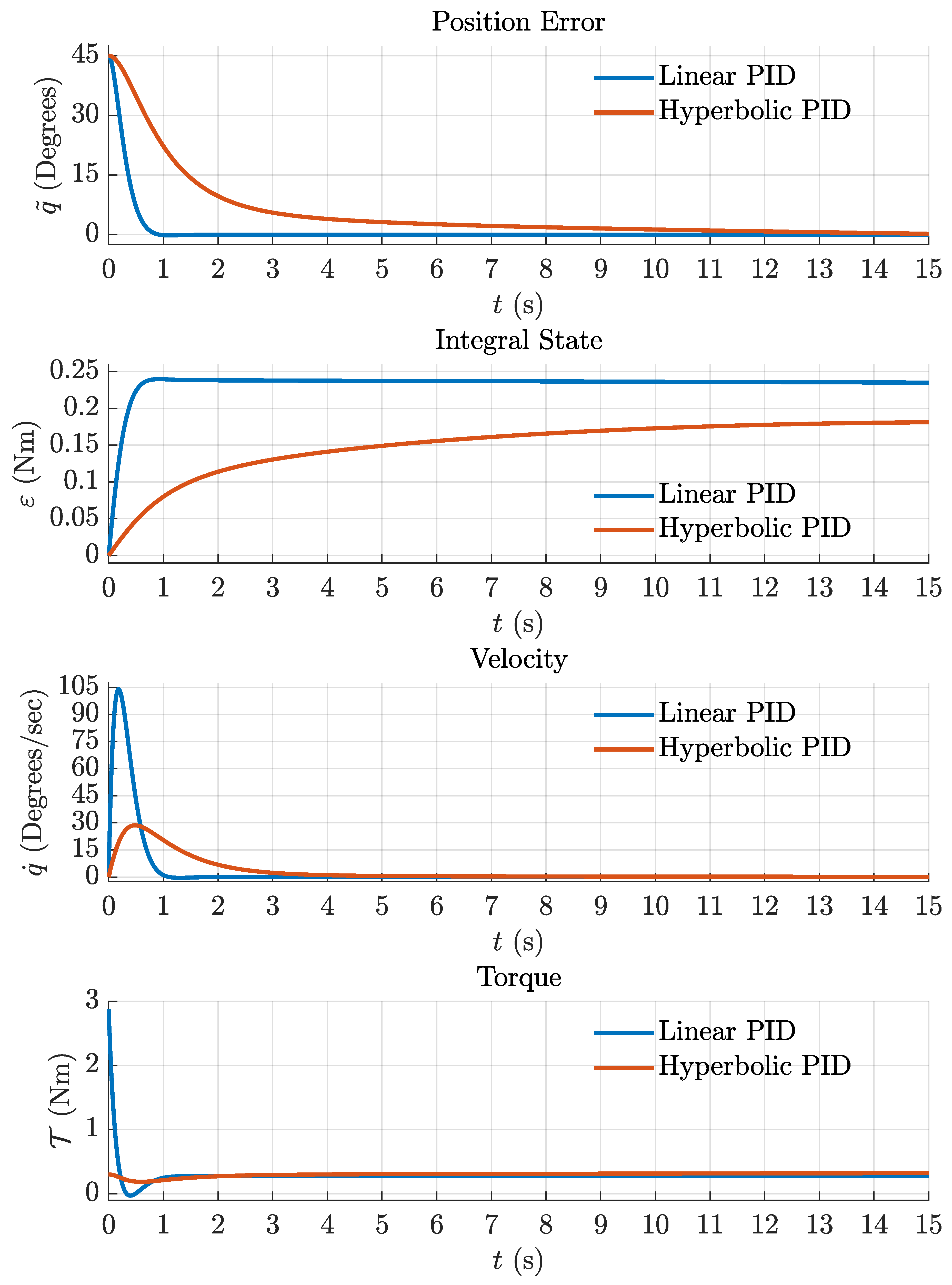
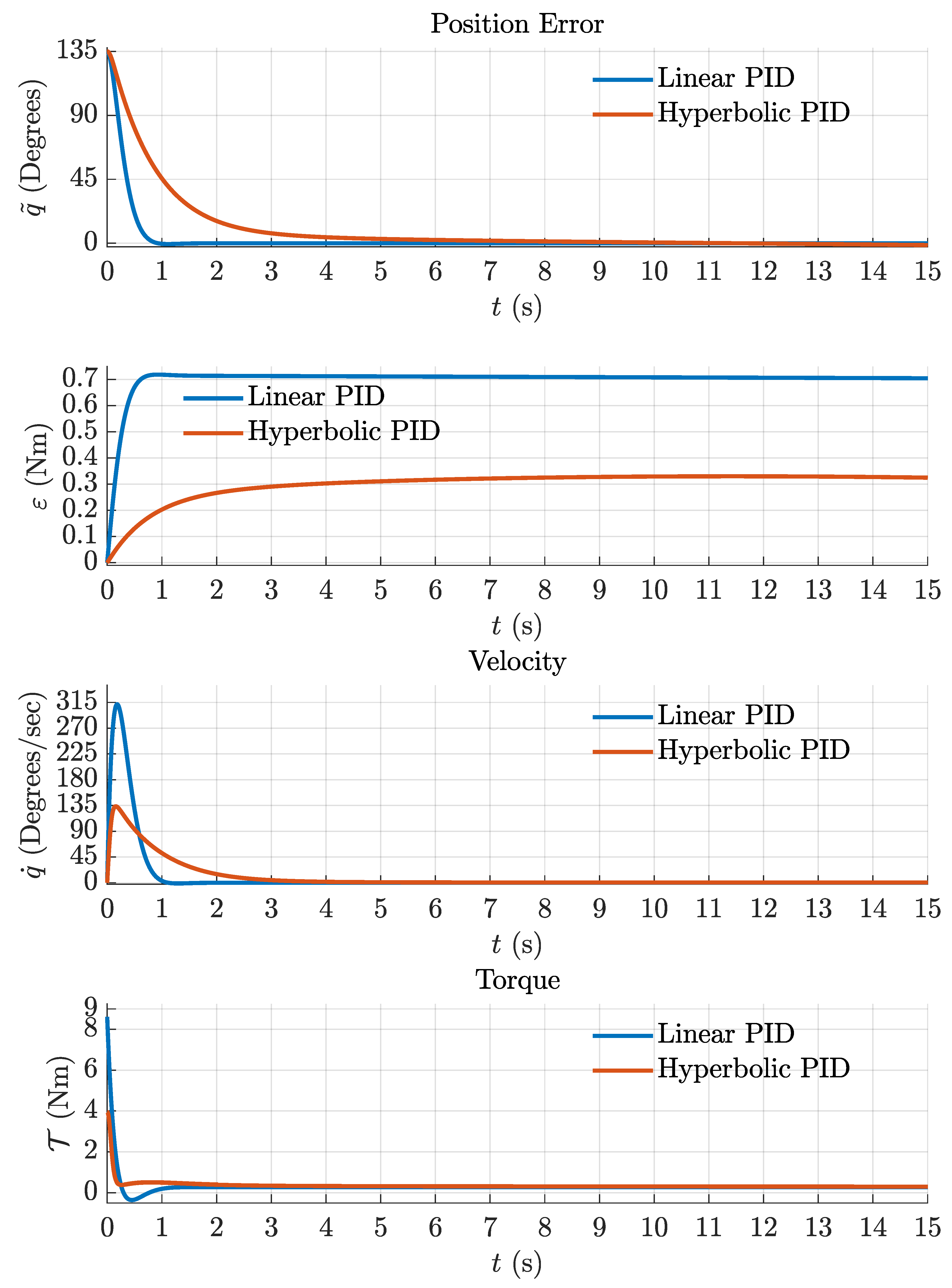
For clarity, in each experiment, the position errors $\tilde{q}\left(t\right)$ and joint velocities $\dot{q}\left(t\right)$ are presented in units of degrees and degrees/s, respectively. The experimental results for the linear PID and the hyperbolic PID-Type control schemes corresponding to the desired reference $q_{d1}={\displaystyle \frac{\pi }{4}}$ rad [45°] are shown in Figure 3. The position error $\tilde{q}\left(t\right)$ under the proposed control exhibits a smooth transient response without vibrations, ripples, or overshoot, and it converges asymptotically to the equilibrium point, with a settling time (time to reach an error $\le 2\%$) of $\sim 11.6300$ s. In contrast, the conventional PID controller achieves a faster transient response than the hyperbolic controller, with a settling time of $\sim 0.7625$ s, but presents a small $\sim 0.4176\%$ overshoot. It also reaches steady state with asymptotic convergence to the equilibrium point. It is important to highlight that the damping demand in the linear PID is much greater than in the hyperbolic case. Therefore, the dissipative effect in the PID (i.e., the conversion of mechanical energy into thermal energy) is larger. This effect is reflected in the transient behavior of the applied torque profiles. The linear PID requires a negative torque to decelerate the pendulum’s movement, whereas in the nonlinear PID, there is no change in polarity, thus avoiding sign switching and providing a smoother energy injection. In both cases, the torque signals remain in the linear operating region and within the physical limits of the servomotor, thereby avoiding saturation. Regarding the integral state, it can be observed that in the hyperbolic PID, ${\epsilon }_h$ rises to a smaller constant value compared to the linear version. This occurs because the integral of the error is evaluated through the saturated hyperbolic function, resulting in a small steady-state control torque.

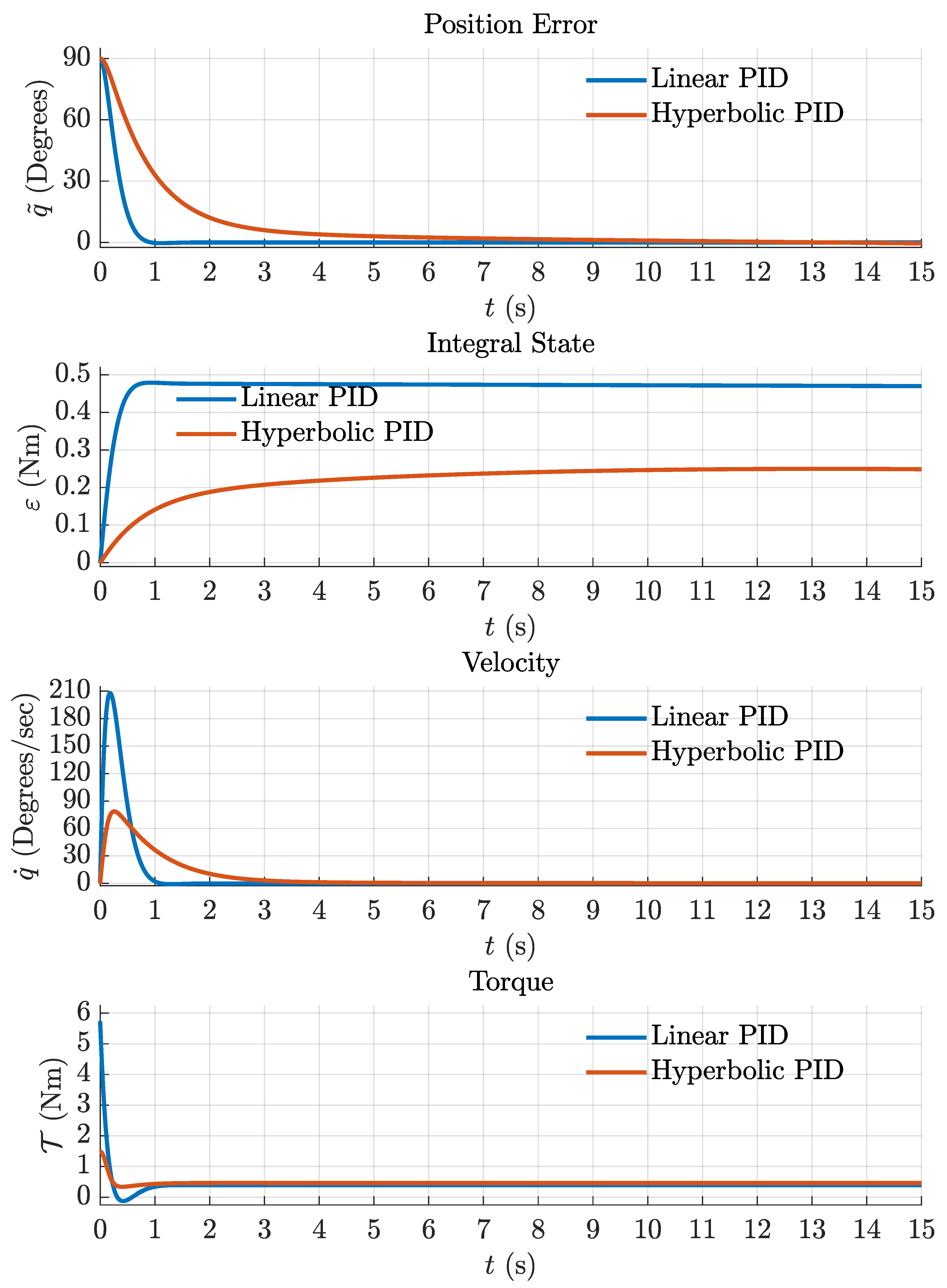
Figure 4 shows the experimental results for the case $q_{d2}={\displaystyle \frac{\pi }{2}}$ rad (90°). Note that both position errors converge asymptotically to the equilibrium point; the transient response of the linear PID is faster than that of the hyperbolic controller, with a settling time of ∼0.7625 s versus ∼7.3075 s. However, the classical PID exhibits a small ∼0.4176% overshoot, whereas the proposed scheme maintains a smooth transient response, as in the previous experiment, with no overshoot, oscillations, or vibrations. The damping injected by the linear PID controller is much greater than the damping applied by the nonlinear PID scheme (as can be seen in the joint velocity profiles). The same trend appears in the integral action, which contributes significantly more to the steady-state torque in the linear PID than in the nonlinear one. A major advantage of the proposed controller is that the applied torques remain within the physical limits of the servomotor, whereas the linear PID computes a torque of $5.8$ Nm, exceeding the 4 Nm limit and causing saturation. This implies that the linear PID cannot maintain its performance with the same gains; that is, re-tuning would be required to correct this issue. In contrast, the hyperbolic algorithm preserves its transient characteristics using the same gains while operating within the linear region of the servomotor. This represents a significant advantage of the proposed scheme over the linear PID.

The experimental results for the case $q_{d3}=3{\displaystyle \frac{\pi }{4}}$ rad [135°] are shown in Figure 5. The proposed hyperbolic PID-type scheme (5) maintains the same performance observed in the previous two experiments: a smooth transient response without overshoot, oscillations, or vibrations, settling time of ∼5.4025 s, together with a mild integral action. The applied torque remains within the saturation limits ($3.8$ Nm < 4 Nm), and the damping injection is reduced. In contrast, the linear PID requires an applied torque that exceeds the saturation limits in order to achieve the necessary dissipative effect during the transient state, and it relies on a much more aggressive integral action to reach steady-state performance, with a settling time of ∼0.7625 s and ∼0.6258% overshoot.

It is very important to observe that the proposed hyperbolic scheme maintains its performance without the need to tune one more time the control gains. Whereas the linear PID gains depend on the desired reference, that is, $k_p=k_p\left(q_d\right)$, this is a well-known characteristic for the simple PID that, at the same time, becomes a disadvantage.

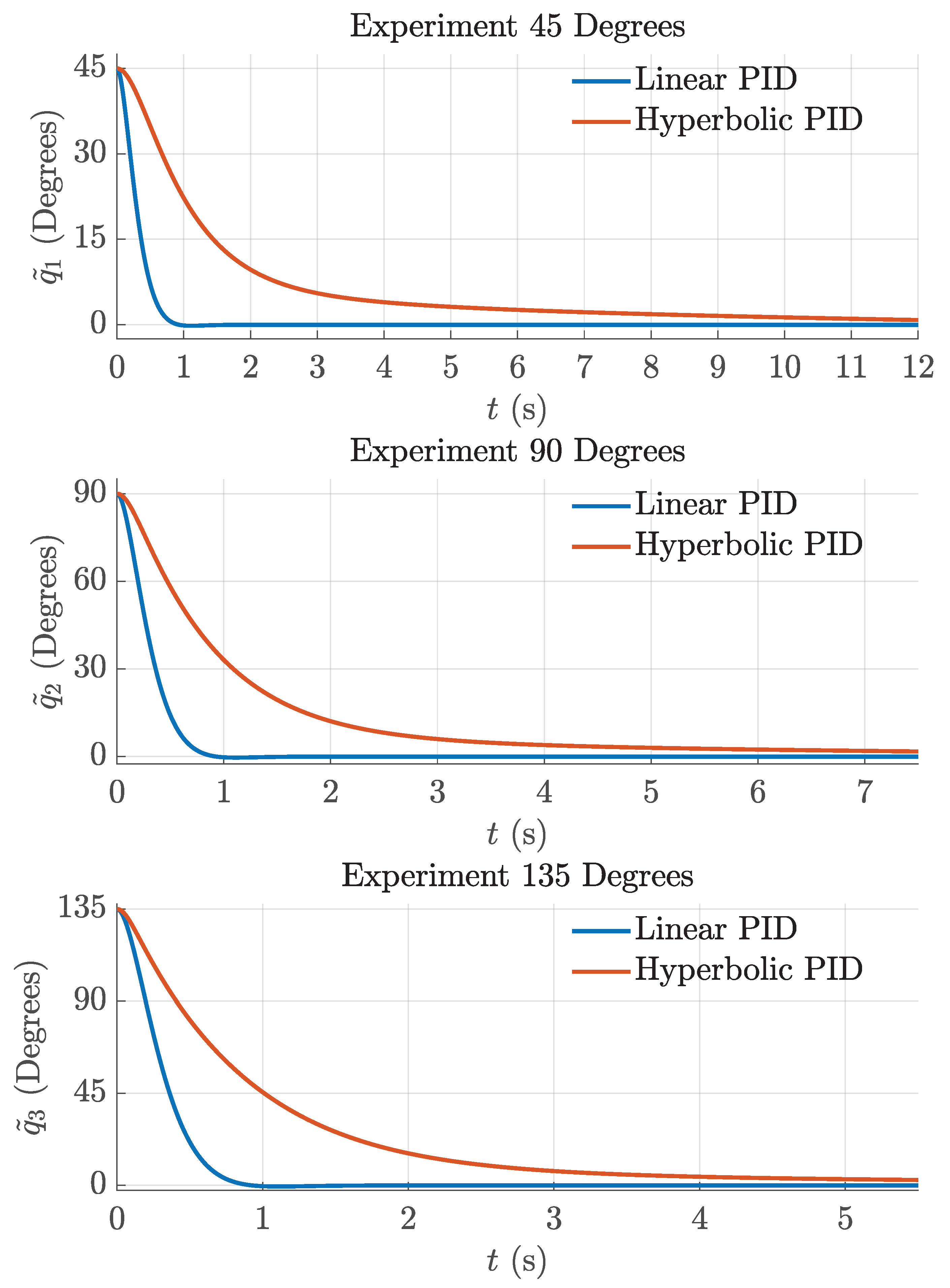
With the purpose of analyzing in greater detail the transient response behavior of linear PID control schemes and the proposed hyperbolic structure, Figure 6 shows the transient states of the position error of both evaluated schemes, corresponding to the three previous experiments.

For the three references evaluated, the hyperbolic scheme exhibits a smooth response, highlighting its exponential effect converging towards zero, without any overshoot, oscillations, ripple, or vibrations, and reaching the steady state smoothly. It is worth noting that these were the best achievable responses for classical PID control; although a tuning method was developed to avoid saturating the applied torques, which the proposed scheme achieves very well, it is not suitable for classical PID control. Therefore, several attempts were made to tune the gains to make it competitive with linear PID control. The tuning method developed also represents a modest contribution, guaranteeing a smooth transient response without overshoots, vibrations, or oscillations. These transient response characteristics were not observed in the few works that experimentally evaluate different types of PID control.

5.3. Remark on Unmodeled Dynamics and Robustness

The dynamic model of the pendulum (1) neglects the dissipative phenomena of static friction, Coulomb friction, and the Stribeck effect. Considering these effects would prevent the establishment of asymptotic stability, relaxing the result to stability and robustness. Another reason dissipative phenomena were not taken into account is that they involve the $\mathrm{sign}(·)$ function (with the exception of viscous friction), which is not a Lipschitz function. To overcome this problem, it would be necessary to compensate for all friction phenomena, which is a different topic from the one addressed in this paper. The above arguments are from a theoretical point of view; however, in practice, these phenomena are present in the pendulum and are reflected in the experimental results. From a practical perspective, friction phenomena in the direct-drive servomotor of the pendulum are very low—particularly static friction, Coulomb friction, and the Stribeck effect—with viscous friction predominating [34].

Figure 6 shows a small edge at the beginning of the transient response in the position error, which corresponds to the Stribeck friction effect. This phase, from the hysteresis zone of static friction to velocity-dependent friction, is not immediate; the Stribeck zone occurs when the motion velocity is very small, where $q\left(t_k\right)\approx 0$. However, this effect has no consequences on the rest of the pendulum’s response.

Future work: the proposed hyperbolic scheme will be extended to the case of an n-DOF robot manipulator.

6. Conclusions

In this work, a rigorous global asymptotic stability analysis of the equilibrium point of the closed-loop system is presented for a Lagrangian dynamics model, such as a pendulum controlled with a linear PID regulator using a strict Lyapunov energy function. This procedure is then generalized to design a new hyperbolic PID-Type control scheme. The conditions for the existence and uniqueness of the equilibrium point of the resulting closed-loop system are established. To prove the global asymptotic stability for the proposed hyperbolic scheme, the strict Lyapunov function employed for the linear PID case is suitably adapted, thereby completing the demonstration.

From the experimental results on a direct-drive pendulum, the effectiveness and performance of the proposed scheme can be confirmed. The transient response under the hyperbolic controller is smooth, without overshoot, vibrations, or oscillations. Moreover, the gain-tuning procedure developed in this work is shown to be easier to apply over a wide range of desired references, while also avoiding torque saturation. In contrast, the classical PID control scheme cannot maintain its performance when the reference changes, leading to servomotor saturation when the same gains are used.