Distributional Drift in IoT Intrusion Detection Systems: Implications for Cross-Dataset Generalisation

Abstract

The rapid expansion of Internet of Things (IoT) technologies has highlighted the need for reliable intrusion detection systems (IDSs), yet the majority of existing studies rely on single-dataset evaluations, raising concerns about their real-world generalisation capability. This study addresses this limitation by systematically investigating distributional shift across heterogeneous IoT intrusion detection datasets and their impact on model behaviour. To achieve this, a unified feature space is constructed using BoT-IoT, ToN-IoT, and UNSW-NB15 datasets, followed by a comprehensive preprocessing pipeline including attack class alignment, distribution-preserving sampling for class imbalance, and feature selection based on cross-dataset feature value propagation analysis. Furthermore, feature-specific transformations and correlation-based dimensionality reduction are applied to enhance statistical consistency and model stability. To simulate realistic deployment scenarios, models are trained on combinations of datasets and evaluated on unseen datasets. The results reveal that distributional inconsistencies and dataset-specific feature biases significantly degrade cross-dataset performance, despite strong within-dataset results. The proposed framework provides a systematic understanding of feature-level behaviour across datasets, identifying both stable and bias-prone features. These findings highlight the necessity of distribution-aware preprocessing and feature analysis for developing robust and generalisable IoT intrusion detection systems.

1. Introduction

The widespread adoption of Internet of Things (IoT) technologies in recent years has led to the emergence of a broad application ecosystem, ranging from smart cities and industrial automation to healthcare systems and smart home devices [1]. Today, billions of IoT devices continuously generate data across diverse network environments, and these devices have become an integral component of modern information systems [2]. However, the substantial growth in the number of IoT devices has also introduced significant security risks. Due to limited computational resources, weak security mechanisms, and heterogeneous network architectures, IoT environments have become highly attractive targets for cyber-attacks [1,3]. In particular, network-based attacks, such as distributed denial-of-service (DDoS) attacks, botnet-based attacks, and reconnaissance activities, pose significant threats to IoT ecosystems [4,5].

In this context, intrusion detection systems (IDSs) are widely regarded as a fundamental component of IoT security. In recent years, machine learning (ML)- and deep learning (DL)-based IDS approaches have become an active research area, leading to the development of state-of-the-art systems that achieve high detection performance across numerous studies [6,7,8].

However, a substantial portion of the performance results reported in the literature are derived from experiments conducted on specific benchmark datasets. This raises an important question regarding the extent to which the developed models can generalise to different data sources or real-world network environments [9,10]. Real IoT networks consist of a wide variety of device types, communication protocols, traffic patterns, and deployment architectures, resulting in highly variable statistical characteristics of network traffic. Consequently, models trained on a single dataset often learn dataset-specific patterns, limiting their ability to generalise effectively across different environments [9,11].

When commonly used datasets are examined in IoT-based IDS (IoT-IDS) research, it becomes evident that each dataset is generated under different network environments, attack scenarios, and traffic generation mechanisms [12]. For instance, while some datasets produce flow-based features, others contain packet-level attributes or statistical characteristics computed over varying time windows [13]. As a result, significant differences emerge across datasets in terms of feature definitions, the number of features, and the statistical computation methods used [14,15]. Consequently, directly combining datasets or utilising them within a single global model becomes highly challenging.

This heterogeneity problem becomes even more pronounced when considering datasets specifically designed for IoT environments. IoT networks are inherently complex systems composed of diverse communication protocols, device types, interaction patterns, and deployment architectures [16]. As a result, different IoT datasets exhibit significant variation not only in attack categories but also in their underlying feature spaces.

Thus, models trained on a particular dataset may suffer substantial performance degradation when evaluated on other datasets, with dataset-specific learning emerging as a key factor limiting the generalisation capability of IoT-IDS models. In machine learning, this phenomenon is commonly associated with drift, which refers to a statistical distributional change between the data on which a model is trained and the data that it encounters during deployment or evaluation (e.g., test data) [17]. The term drift is used to describe changes that arise when a model trained in one context is applied in a different context [18], often resulting in degradation of predictive performance and loss of reliability [18,19]. This degradation fundamentally stems from statistical discrepancies between training and testing data distributions, where learned patterns no longer align with those observed at inference time.

Considering these challenges, and given that the ToN-IoT, BoT-IoT, and UNSW-NB15 datasets were constructed under different experimental setups and for distinct purposes, performing a drift/shift analysis prior to building a global IoT-IDS is deemed beneficial. Accordingly, such analyses are conducted as a preliminary step to better characterise cross-dataset discrepancies and to support the development of a more robust and generalisable detection framework.

In the literature, several studies have been proposed to address this problem by integrating different datasets into a common feature space in order to develop more generalisable IDS models [20,21]. These approaches typically rely on the reprocessing of raw network traffic, the extraction of unified flow-based features, or the construction of compatible feature representations across datasets.

However, a substantial portion of existing studies fail to provide a comprehensive analysis of the distributional differences across datasets or to examine how feature values behave when transferred between different datasets. In particular, whether specific features retain consistent semantic meaning across datasets or encode dataset-specific biases remains unexplored in the literature.

In parallel, a significant body of the literature has focused on improving intrusion detection performance through the use of advanced machine learning and deep learning models. Tree-based ensemble methods, convolutional neural networks, recurrent neural networks, and hybrid architectures are among the commonly adopted approaches in this field [6,22].

In addition to model development, other studies have explored feature engineering, dimensionality reduction, or sampling strategies to address challenges such as high dimensionality, class imbalance, and noisy data [10,23,24]. Furthermore, several works propose new preprocessing pipelines or feature selection techniques aimed at improving model accuracy and computational efficiency [25,26,27].

Despite these efforts, the majority of these studies are evaluated on a single dataset, with structural differences across datasets largely overlooked [7,28,29].

In recent years, several studies have attempted to address the cross-dataset generalisation problem by developing more robust IDS models capable of operating in heterogeneous environments [30,31,32]. These approaches typically rely on strategies such as constructing a unified feature space, reprocessing raw network traffic, or applying domain adaptation techniques to mitigate distributional differences across datasets [28,33,34].

Recent studies have begun to address related aspects of this problem from complementary directions. Semenov et al. [35] proposed a preprocessing method combining correlation reduction via a PCA-based procedure and the SMOTEENN balancing algorithm [36], demonstrating improved classification performance on a single IDS benchmark dataset. While their work highlights the importance of preprocessing for model quality, it does not examine cross-dataset behaviour or the extent to which preprocessing decisions affect distributional consistency across heterogeneous data sources. Cantone et al. [37] conducted a comprehensive cross-dataset generalisation study across four network intrusion detection datasets, reporting a severe performance gap between within-dataset and cross-dataset evaluation, with the average MCC (Matthews Correlation Coefficient [38]) dropping from approximately 94% to 29%. Their analysis confirms that trained models fail to transfer learned patterns to unseen datasets, and visualisation techniques are employed to illustrate distributional differences. However, their study does not identify which specific features encode dataset-specific biases or quantify distributional shift at the feature-value level, and the datasets considered do not include IoT environments. The present study addresses these gaps by introducing a cross-dataset feature value propagation analysis that identifies the root causes of generalisation failure at the feature and value levels, and by applying multiple complementary drift metrics to systematically quantify distributional shift across heterogeneous IoT intrusion detection datasets.

Nevertheless, the extent to which feature values propagate across datasets, as well as whether certain features encode dataset-specific biases, remains poorly characterised in the literature. Therefore, a systematic analysis of the behaviour of cross-dataset features is necessary to better understand the sources of dataset-specific bias and improve the generalisability of IoT-IDS models.

In this study, a multi-dataset scenario is considered to design more realistic and generalisable IoT-based intrusion detection systems. Multiple IoT and IDS datasets collected from different network environments are analysed within a common feature space, and the effects of distributional shift on machine learning model behaviour are systematically investigated.

Within this framework, a drift–shift analysis is conducted at the feature level to examine how statistical properties and dominant feature values vary across datasets. This analysis aims to identify dataset-specific biases and distributional inconsistencies that may negatively affect the generalisation capability of intrusion detection models when applied to unseen environments.

The primary objective of this approach is to better understand the sources of distributional shift between IoT intrusion detection datasets, reduce dataset-specific biases, and develop an IoT intrusion detection model that operates more reliably across heterogeneous data sources. To achieve this, a series of preprocessing and analytical steps are applied, including the joint analysis of multiple datasets under a unified representation, handling class imbalance, and investigating distributional characteristics of features across datasets.

The main contributions of this study can be summarised as follows:

• A systematic investigation of the feature space heterogeneity and distributional shift problem across IoT and IDS datasets.
• A feature-level drift–shift analysis framework for examining how statistical properties of features change across different datasets.
• The development of a comprehensive experimental framework for evaluating the generalisation capability of intrusion detection models in a multi-dataset setting.
• A detailed evaluation of how dataset-specific biases and distributional differences influence the behaviour of machine learning-based intrusion detection systems.

The remainder of this paper is organised as follows: Section 2 introduces the IoT and IDS datasets considered in this study, provides important details of the preprocessing procedures, and presents the proposed feature-level drift–shift analysis framework. Section 3 reports the experimental results and provides a comprehensive discussion of distributional shift patterns across both traditional machine learning and deep learning configurations. Finally, Section 4 concludes the paper by summarising the key findings and outlining directions for future research on cross-dataset generalisation and robust IoT-IDS.

2. Materials and Methods

2.1. Methodology Overview

Figure 1 presents an overview of the proposed methodology. The pipeline begins with three heterogeneous IoT intrusion detection datasets (BoT-IoT, ToN-IoT, and UNSW-NB15), which are first unified into a common feature space through attack class alignment and a shared NetFlow-based representation. To address the severe class imbalance present across all datasets, the KLSampler undersampling method is applied, preserving the underlying distributional structure of each class. The resulting datasets are then subjected to a four-step preprocessing pipeline comprising variance-based constant feature removal, cross-dataset feature value propagation analysis, multicollinearity-based dimension reduction by using Random Forest importance, and feature-specific transformations including logarithmic scaling, clipping, and supervised binning. Following preprocessing, a comprehensive drift–shift analysis is conducted using four different statistical metrics alongside visual analysis techniques. Finally, two methodologically distinct models are trained and evaluated under cross-dataset conditions to assess the impact of distributional shift on generalisation performance. Each of the steps is described in detail in the following sections.

2.2. Dataset Selection

In both classical machine learning and modern deep learning paradigms, the generalisation capability of a model across multiple data sources is fundamentally determined by the structure and consistency of the underlying feature space. In scenarios where multiple datasets are combined for training or a single global model is expected to operate across heterogeneous data sources, it is implicitly assumed that all input features share a common semantic meaning. When this assumption is violated, the learned decision boundaries become dataset-specific, resulting in degraded performance and unreliable predictions when the model is applied to unseen data from different sources. Consequently, the existence of a shared and consistent feature space is a prerequisite for integrated and transferable learning.

This problem becomes more evident in the context of IDSs and IoT-IDSs. Most popular benchmark datasets demonstrate that the construction of each dataset is motivated by distinct goals, traffic generation conditions, and data collection workflows. For example, one of the first standardised testbeds for intrusion detection systems is the DARPA98 dataset that was created by MIT’s Lincoln Laboratory under the sponsorship of DARPA [39]. It includes artificial benign network traffic, along with 38 distinct attack types, which were captured in raw TCP/IP header data as well as in time sequence using tcpdump [40]. DARPA98 provided a baseline benchmark for IDSs in the past, but it fails for current networks with high levels of heterogeneity and complexity.

Derived from the processed network traffic portion of DARPA98, the KDD’99 dataset represents each connection using 41 features and has been widely used in IDS studies [41]. However, because KDD’99 contains a significant number of duplicate records, it introduces a strong bias toward high-frequency patterns, resulting in overoptimistic performance estimates. To address these limitations, the NSL-KDD dataset was introduced, in which duplicate records were removed to rebalance the data distribution, providing a more challenging and fair framework for evaluating classification algorithms [42]. However, both datasets are still derived from traditional traffic features and lack representation of contemporary attack behaviours.

To better represent modern cyber threats, newer datasets such as UNSW-NB15 and CICIDS2017 have been proposed. The UNSW-NB15 dataset was created using the IXIA PerfectStorm traffic generator, combining real benign programmes with 9 different modern attack families. Argus and Bro-IDS (Zeek) are used for extracting features from raw Packet Capture (PCAP) files, resulting in a total of 49 features [43]. In contrast, the CICIDS2017 dataset, released by the Canadian Institute for Cybersecurity, includes seven well-known attack families (including brute force, DoS/DDoS, web attacks, botnet, and infiltration, as well as Heartbleed). It provides more than 80 flow-based traffic features per network connection, computed using its proprietary tool, CICFlowMeter [44].

IoT-orientated datasets further exacerbate the feature space heterogeneity due to the diversity of devices, protocols, and deployment architectures. The ToN-IoT dataset was designed to represent complex and heterogeneous IoT environments by incorporating edge, fog, and cloud layers, as well as data from network traffic, operating system telemetry, and user-level activities [45]. It includes nine distinct attack types and provides a rich multi-source representation. The BoT-IoT dataset focuses on large-scale botnet-driven IoT attack scenarios and relies on flow-based features extracted using the Argus tool, with an emphasis on high-volume and high-velocity traffic patterns [46]. The IoT-23 dataset captures long-duration traffic traces from real IoT devices and malware scenarios, offering realistic behavioural insights; however, its feature definitions and labelling schemes are not directly compatible with other IDS benchmarks [47]. Similarly, the N-BaIoT dataset was developed in the context of autoencoder-based intrusion detection and concentrates on Mirai and Bashlite attacks, producing high-dimensional statistical representations with 115 features but limited attack diversity [48].

As summarised in

Table 1. Summary of classical and contemporary IDS and IoT datasets.

Category	Dataset	Tool	Number of Records	Feature Count	Classes
Classical IDS	DARPA98 [39]	tcpdump	4,900,000	41	5
	KDD Cup 99 [41]	tcpdump	4,898,431	41	5
	NSL-KDD [42]	tcpdump	148,517	41	5
	CICIDS2017 [44]	CICFlowMeter	2,830,743	78	15
	UNSW-NB15 [43]	Argus/Bro	2,540,044	49	10
IoT-focused IDS	ToN-IoT [45]	Zeek	223,390,210	46	9
	BoT-IoT [46]	Argus	73,370,443	48	6
	IoT-23 [47]	Zeek	325,397,990	23	8
	N-BaIoT [48]	–	849,234	115	2

Classical IDS datasets mainly rely on enterprise network traffic captured via packet-level or flow-level tools, whereas IoT-focused datasets emphasise large-scale, heterogeneous device communications and protocol diversity typical of IoT environments.

, although each of these datasets provides internally consistent and well-defined feature representations, differences in PCAP tools, flow aggregation mechanisms, time window definitions, and statistical computation strategies lead to fundamentally incompatible feature spaces. As a result, the original CSV files cannot be directly merged or jointly utilised to train a single global IDS model. This structural incompatibility represents a major barrier to cross-dataset generalisation, integrated threat modelling, and the development of scalable IDS solutions for heterogeneous environments.

To overcome these limitations and fully leverage the rich information contained in existing IDS and IoT-IDS datasets, it is essential to revisit feature space design, establish a shared representation across datasets, and develop learning frameworks that explicitly address feature-level heterogeneity.

To address this challenge, it is necessary to combine multiple datasets collected from different network environments and experimental conditions. However, as discussed previously, widely adopted IDS datasets are constructed using diverse traffic generation scenarios, PCAP approaches, and feature extraction processes, resulting in structurally incompatible feature spaces.

Therefore, a direct integration of raw data or original CSV representations is not feasible. This necessitates the development of a unified feature representation that enables joint analysis across datasets and supports the training of a global intrusion detection model.

This limitation is explicitly addressed by Sarhan et al. [21], who propose a unified feature space for consistent and comparable analysis of IDS datasets. In their approach, raw network traffic traces from multiple datasets are obtained in PCAP format and subsequently transformed into CSV files with a shared feature representation using the flow-based NetFlow analysis tool [49]. The resulting datasets, aligned within a common feature space, are made publicly available for research purposes [21].

Through this transformation, datasets collected from heterogeneous network environments and attack scenarios can be analysed within a consistent representational framework, ensuring uniform feature definitions, statistical computation methods, and flow abstractions. Thus, the impact of structural differences between datasets on model behaviour is significantly reduced. Building on this approach, we utilise these standardised datasets to address feature space incompatibility in IDS and IoT-IDS research. In particular, widely used and recent datasets (including ToN-IoT, BoT-IoT, and UNSW-NB15) are incorporated within this unified representation to enable a comprehensive evaluation of global IoT intrusion detection models.

2.3. Unification of Intrusions and Handling Imbalance

Since intrusion detection datasets are collected from heterogeneous network environments and are designed to reflect different threat models and experimental objectives, they naturally contain diverse and only partially overlapping attack taxonomies. However, supervised learning models rely on the assumption that class labels are consistent between training and evaluation.

When an attack class is present in the test data but absent in the training data, the model may incorrectly classify unseen attack types as known classes, leading to misleading performance estimates. Conversely, if an attack class is included during training but does not appear in the test set, it becomes impossible to assess the model’s performance for that class.

Therefore, to ensure a valid and interpretable evaluation of ML- and DL-based IDS models, the label space used during training and testing must be aligned. In a multi-dataset learning setting, this requires identifying a common subset of attack categories shared across datasets. Accordingly, in this study, only attack types that are present in at least two of the selected datasets (namely, ToN-IoT, BoT-IoT, and UNSW-NB15) are considered as the target classes of the proposed IoT-IDS model. This approach follows a closed-set classification assumption enabling a consistent evaluation of how well the model generalises across datasets.

The datasets obtained from Sarhan et al. [21] are considerably large, posing practical challenges for model training. In particular, the BoT-IoT and ToN-IoT datasets contain 37,763,497 and 16,940,496 records, respectively, corresponding to approximately 6 GB and 2.86 GB of storage. The direct use of these datasets may cause practical difficulties from two perspectives: The utilisation of these large-scale datasets introduces practical difficulties, as it can lead to excessively long training times, especially for classical machine learning models, and may also result in memory limitations that hinder model training [50]. Furthermore, a review of existing studies shows that most works rely on reduced subsets—typically around 5% of the full datasets—provided by the original authors.

Following this common practice, the NetFlow-based datasets used in this study were reduced to their 5% subsets. This reduction decreased the size of the BoT-IoT dataset to 2.13 GB and the ToN-IoT dataset to 84.2 MB, making them more suitable for practical experimentation while remaining consistent with prior work.

Finally, after applying attack class unification and data reduction, the selected classes for this study are summarised in

Table 2. Distribution of selected attack classes across datasets.

Attack Class	BoT-IoT	ToN-IoT	UNSW-NB15
Normal/Benign	135,037 (1.00%)	57,614 (18.30%)	2,295,222 (99.20%)
DoS	4,514,065 (33.37%)	21,384 (6.79%)	5794 (0.25%)
DDoS	8,815,828 (65.16%)	235,740 (74.90%)	–
Reconnaissance	62,504 (0.46%)	–	12,779 (0.50%)
Total Samples	13,527,509	314,738	2,313,795

.

As shown in Table 2, the datasets exhibit severe intrusion imbalance. In the BoT-IoT dataset, DDoS attacks account for 65.16% of all records, while DoS represents 33.37%, and reconnaissance attacks comprise only 0.46%. Similarly, in the ToN-IoT dataset, DDoS attacks dominate the distribution, with 74.90% of the records, whereas DoS accounts for only 6.79% and reconnaissance attacks are present at a negligible level. In contrast, the UNSW-NB15 dataset is heavily skewed toward normal traffic, with 99.20% of the records labelled as benign and attack classes representing only a small fraction.

When training models on such imbalanced datasets, they tend to focus on dominant classes, leading to poor learning of minority classes. This imbalance can result in overfitting to majority classes and underfitting of minority classes, ultimately producing misleading evaluation metrics, such as inflated accuracy [51].

To address these issues, we apply the KLSampler undersampling methodology that we proposed previously elsewhere [52]. Unlike the conventional undersampling approaches, KLSampler resamples the data by measuring the distributional differences between the undersampled and original data by using Kullback–Leibler (KL) divergence, and it explicitly aims to minimise this discrepancy. In the initial stage, the algorithm employs k-means clustering to identify high-density regions within the majority class and selects a proportionally representative subset. Subsequently, using kernel density estimation (KDE), this method iteratively increases the sampled subset by adding instances that progressively reduce the KL divergence between the sampled and original class distributions. Through this process, the method mitigates class imbalance while preserving the underlying data distribution, ensuring that key statistical characteristics in the data are maintained across different intrusion scenarios.

Table 3. Distribution of selected attack classes across datasets after KLSampler.

Attack Class	BoT-IoT	ToN-IoT	UNSW-NB15
Normal/Benign	135,037 (20.61%)	57,614 (27.14%)	61,103 (76.68%)
DoS	228,310 (34.83%)	21,384 (10.07%)	5794 (7.20%)
DDoS	229,516 (35.03%)	133,245 (62.77%)	–
Reconnaissance	62,504 (9.54%)	–	12,779 (16.03%)
Total Samples	655,442	390,746	156,156

shows the distribution of the classes across the datasets after KLSampler is applied.

The results demonstrate that KLSampler effectively reduces class dominance and yields more balanced datasets. In the BoT-IoT dataset, the proportions of DDoS and DoS classes are decreased to 35.03% and 34.83%, respectively, while Normal/Benign and Reconnaissance increase to 20.61% and 9.54%, respectively. In the ToN-IoT dataset, the proportion of DDoS attacks decreases from 74.90% to 62.77%, with DoS adjusted to 10.07% and Normal/Benign traffic increasing to 27.14%. For the UNSW-NB15 dataset, the proportion of Normal/Benign traffic is reduced from 99.20% to 76.68%, thereby substantially increasing the relative representation of attack classes, with reconnaissance attacks reaching 16.03%. Overall, these results indicate that KLSampler produces more balanced class distributions across all of the datasets.

To further validate the effectiveness of the sampling process, Figure 2 presents the processing time and resulting data size for each dataset–attack pair. These results demonstrate that KLSampler achieves distributional balancing while maintaining computational efficiency and manageable dataset sizes.

2.4. Data Preprocessing

Following dataset balancing, a preprocessing pipeline was applied to all feature sets prior to drift analysis and downstream model training. The pipeline was designed to improve data quality, remove redundant signals, and produce a well-conditioned feature space suitable for robust learning. First, zero-variance and near-zero-variance features were removed, as they do not contribute meaningful information and may negatively affect model performance [53,54]. In addition, feature value propagation analysis was used to identify less informative or redundant features not captured by variance-based filtering [55].

Next, multicollinearity among the remaining features was assessed, and highly correlated features were reduced to improve model stability and generalisability [56,57,58,59].

Finally, exploratory analysis was performed to examine feature distributions, and appropriate transformations, such as min–max scaling, standardisation, and normalisation, were applied where necessary.

As the primary focus of this study is the analysis of covariate shift across datasets, the full preprocessing details are provided in the Supplementary Materials (Section S1).

To prevent information leakage, all of these steps are derived exclusively from the training split of each experimental configuration and subsequently applied to the test set using the parameters and thresholds fitted on the training data.

2.5. Drift–Shift Analysis

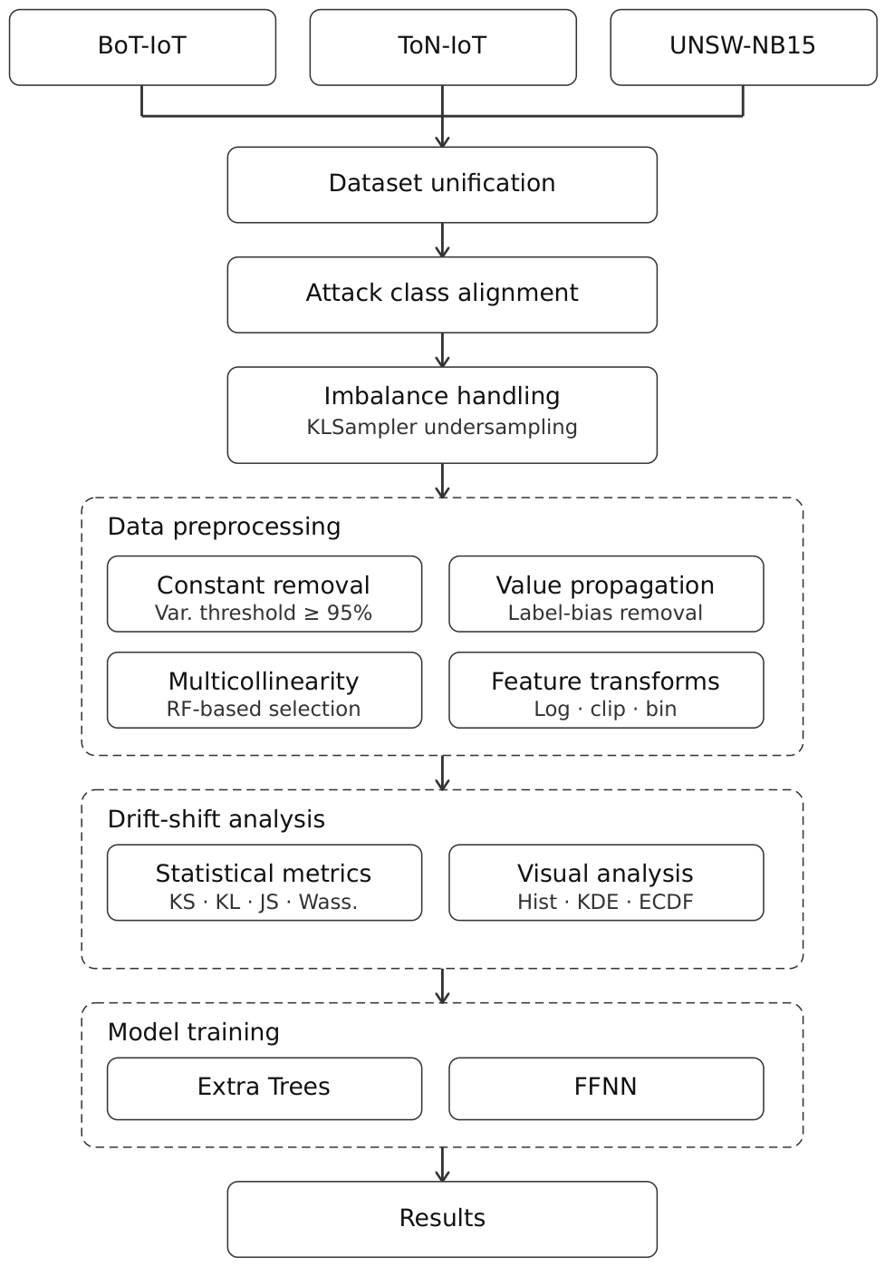
To systematically quantify distributional discrepancies across datasets, a comprehensive drift and shift analysis was conducted. Given that the datasets under consideration originate from different environments and experimental setups, understanding the nature and magnitude of these discrepancies is critical for evaluating cross-dataset generalisation. To this end, the analysis was structured in two stages: First, a set of complementary statistical metrics were introduced to capture different aspects of distributional change. Subsequently, these metrics were applied across multiple dataset combinations to empirically examine feature-level drift and its implications for model robustness.

2.5.1. Drift–Shift Detection Metrics

To assess drift–shift between training and evaluation datasets in a systematic and interpretable manner, multiple complementary drift metrics were employed. Each metric captures a distinct aspect of distributional change, enabling a robust and multi-perspective analysis of feature-level stability across datasets.

Kolmogorov–Smirnov (KS) Test: The Kolmogorov–Smirnov test is a non-parametric statistical test that quantifies the maximum difference between the empirical cumulative distribution functions (ECDFs) of two samples. It directly measures structural changes in distribution shape without making assumptions about the underlying data distribution. The KS statistic is defined as follows:

$$D=\underset{x}{sup}\left|F_1\left(x\right)-F_2\left(x\right)\right|,$$

(1)

where $F_1\left(x\right)$ and $F_2\left(x\right)$ denote the ECDFs of the training and test datasets, respectively. In this study, KS is primarily used as a fast and interpretable first-pass indicator of global distributional shift.

Kullback–Leibler Divergence: Kullback–Leibler (KL) divergence is asymmetric and particularly sensitive to rare events and unseen behaviours, making it suitable for identifying asymmetric or emergent distributional shifts. The KL divergence measures the information loss incurred when one probability distribution is used to approximate another. For discrete probability distributions, it is defined as follows:

$$D_{KL}(P\Vert Q)=\sum _{x}P\left(x\right)log{\displaystyle \frac{P\left(x\right)}{Q\left(x\right)}}.$$

(2)

Jensen–Shannon Divergence: Jensen–Shannon (JS) divergence is a symmetric and bounded variant of KL divergence that quantifies how much two distributions deviate from their shared mean distribution:

$$M\left(x\right)=\frac{1}{2}\left(P\left(x\right)+Q\left(x\right)\right),$$

(3)

$$D_{JS}(P\Vert Q)=\frac{1}{2}{D}_{KL}(P\Vert M)+\frac{1}{2}{D}_{KL}(Q\Vert M).$$

(4)

Since JS divergence is bounded in $[0,1]$ and numerically stable, it is well suited for comparative analyses across multiple features and datasets.

Wasserstein Distance: The Wasserstein distance (Earth Mover’s Distance) quantifies the geometric cost of transforming one distribution into another by comparing their quantile functions:

$$W_1(P,Q)={\int }_0^1\left|F_P^{-1}\left(u\right)-F_Q^{-1}\left(u\right)\right|du.$$

(5)

Unlike KS- or KL-based measures, Wasserstein distance explicitly captures shifts in mean, variance, and tail behaviour, making it particularly effective for continuous numerical features.

We employed a combination of KS, KL, JS, and Wasserstein metrics to capture different types of distributional shift. KS highlights structural shape changes, KL emphasises asymmetric and rare-event deviations, JS provides a stable similarity measure, and Wasserstein captures geometric displacement. Together, these metrics offer a comprehensive view of distributional changes across features.

Based on the characteristics and interpretability of these metrics, severity thresholds were defined to support consistent interpretation of distributional shifts. 

Table 4. Severity thresholds for distributional shift metrics.

Drift Level	KS	KL	JS	Wasserstein
Low	<0.1	<0.1	<0.05	<0.1
Moderate	0.1–0.3	0.1–1	0.05–0.2	0.1–0.3
High	0.3–0.6	1–5	0.2–0.4	0.3–0.6
Severe	>0.6	>5	>0.4	>0.6

summarises the threshold ranges used to categorise drift severity levels across all metrics. Evaluating these metrics alongside the defined thresholds provides a unified framework for assessing feature-level stability and identifying features that require transformation, binning, or further preprocessing.

2.5.2. Drift–Shift Analysis Among the Datasets

Using the metrics described in Section 2.5, distributional shift analysis was conducted for seven different experimental settings. These experimental groups can be summarised as follows:

• BoT-IoT Train, ToN-IoT Test;
• BoT-IoT Train, UNSW-NB15 Test;
• ToN-IoT Train, BoT-IoT Test;
• ToN-IoT Train, UNSW-NB15 Test;
• BoT-UNSW Train, ToN-IoT Test;
• ToN-UNSW Train, BoT-IoT Test;
• BoT-ToN Train, UNSW-NB15 Test.

Given that the UNSW-NB15 dataset contains a substantially smaller number of samples compared to the other datasets, it was excluded from the individual training sets of the experiments to avoid potential bias and instability.

This section focuses on a representative scenario in which the training set is formed by the combination of the BoT-IoT and UNSW-NB15 datasets, while the ToN-IoT dataset is used as the test set. This scenario is representative of the analyses that can be performed for the remaining experimental configurations. Detailed tabular results and extended visual analyses for all dataset combinations are provided in the Supplementary Materials (Section S2 and Section S3, respectively). 

Table 5. Feature-level drift metrics between BoT-UNSW train and ToN-IoT.

Feature	KS	KL	JS	Wasserstein
MIN_IP_PKT_LEN_BIN	0.8084	16.0188	0.3857	2.1003
DST_TO_SRC_SECOND_BYTES_LOG	0.7212	9.0025	0.3602	3.2155
OUT_BYTES_LOG	0.7211	15.7417	0.3607	2.0716
SHORTEST_FLOW_PKT_BIN	0.5777	27.9394	0.4032	2.9368
OUT_BYTES_IS_ZERO	0.5315	36.4804	0.1797	0.5315
L4_SRC_PORT	0.5129	0.0014	0.2397	15,579.8899
TCP_WIN_MAX_IN_BIN	0.4479	11.4953	0.1186	0.4646
MAX_IP_PKT_LEN_LOG	0.4172	18.7963	0.1675	1.2089
LONGEST_FLOW_PKT_LOG	0.4172	11.0865	0.3070	2.0828
NUM_PKTS_UP_TO_128_BYTES_LOG	0.4029	12.8595	0.1695	0.6641
SRC_TO_DST_SECOND_BYTES_LOG	0.3951	10.7240	0.5074	0.9576
L4_DST_PORT	0.3727	0.0005	0.0645	5,567.6204
DURATION_BIN	0.3378	3.6909	0.1283	2.1921
IN_BYTES_LOG	0.3351	26.6470	0.5103	2.3413
L7_PROTO	0.3171	1.1218	0.3127	41.8513
SRC_TO_DST_AVG_THROUGHPUT	0.2830	0.0000	0.0008	258,202.4978
TCP_FLAGS	0.2478	0.2415	0.2805	5.3837
FLOW_DURATION_IS_ZERO	0.1441	2.2573	0.1711	0.1711
OUT_BYTES_HIGH_BURST	0.0765	1.1577	0.0602	0.0765
DST_TO_SRC_SECOND_BYTES_HIGH_BURST	0.0394	0.6586	0.0036	0.0394

shows the drift values obtained using different drift metrics.

Table 5 evaluates distributional deviations across multiple features using our four statistical metrics. The results indicate that, for nearly all features, substantial distributional shift is observed between the source and target datasets. This finding suggests that the data distribution on which the model is trained may no longer reflect the target environment and may negatively impact generalisation performance.

In particular, the MIN_IP_PKT_LEN_BIN feature shows drift, with KS (0.8084), KL (16.0188), and JS (0.3857) values indicating severe distributional divergence. Similarly, the SHORTEST_FLOW_PKT_BIN feature demonstrates significant information-theoretic drift, with a KL divergence of 27.9394 and a JS divergence of 0.4032. These features reflect substantial changes in packet-level traffic behaviour across datasets.

Traffic volume-related features such as OUT_BYTES_LOG and DST_TO_SRC_SECOND_BYTES _LOG also exhibit high drift levels, with KL values of 15.7417 and 9.0025 and JS values of 0.3607 and 0.3602, respectively. These results indicate pronounced differences in network load characteristics between the source and target domains. Moreover, binary-derived features such as OUT_BYTES_IS_ZERO (KL: 36.4804), IN_BYTES_LOG (KL: 26.6470), and FLOW_DURATION_IS_ZERO also indicate substantial drift, highlighting changes in fundamental traffic presence patterns.

Several features display particularly large deviations when evaluated using the Wasserstein distance. For example, SRC_TO_DST_AVG_THROUGHPUT yields near-zero KL and JS values, yet its Wasserstein distance reaches 258,202.4978, indicating major geometric shifts in feature values. Similarly, L4_SRC_PORT (15,579.8899) and L4_DST_PORT (5,567.6204) demonstrate substantial positional drift that is not readily captured by entropy-based metrics. These observations emphasise the necessity of incorporating geometric distance measures alongside distributional similarity metrics.

Protocol-, flag-, and duration-related features such as L7_PROTO, TCP_FLAGS, DURATION_ BIN, and NUM_PKTS_UP_TO_128_BYTES_LOG show moderate levels of drift (e.g., for L7_PROTO: KL = 1.1218, JS = 0.3127, Wasserstein = 41.8513). Although less extreme, these deviations indicate shifts in protocol usage patterns and session characteristics that may still influence model behaviour.

Only a limited number of features, such as DST_TO_SRC_SECOND_BYTES_HIGH_BURST and OUT_BYTES_HIGH_BURST, show relatively low drift values, suggesting a degree of stability. However, such features constitute exceptions rather than the norm across the feature space.

Overall, the analysis reveals the presence of widespread and multi-dimensional distributional shift across the examined datasets. Significant changes are observed not only in distributional shape (KS, JS) but also in value-level geometry (Wasserstein), while KL divergence highlights substantial information-theoretic discrepancies. These findings clearly indicate that a model trained on one dataset may fail to maintain reliable performance in target environments, posing a critical challenge for the deployment of a global-scale IoT-IDS.

2.5.3. Visual Representation of the Drift–Shift Among the Datasets

In order to better understand the magnitude and characteristics of distributional shift, we do not rely solely on numerical metrics but also leverage the power of visual analysis. For the constructed experimental setups, multiple graphical techniques are employed to analyse the differences between data distributions from complementary perspectives. Specifically, histogram plots, KDE, ECDF, and KDE difference plots are utilised. Each visualisation method is designed to highlight a different aspect of the distributional discrepancy.

Histogram plots provide a discretized approximation of the distribution of a continuous random variable by partitioning the data into bins. For a sample $X=\{x_1,x_2,\dots ,x_n\}$, the histogram estimate for a bin B can be defined as follows:

$${\widehat{p}}_B={\displaystyle \frac{1}{n}}{\displaystyle \sum _{i=1}^n}1(x_i\in B)$$

(6)

where $1(·)$ denotes the indicator function. Comparing histograms of training and test datasets allows for a direct inspection of shifts in shape, spread, and concentration regions. However, since histograms are sensitive to bin selection, a smoother representation is achieved through KDE.

KDE provides a non-parametric estimate of the underlying probability density function, yielding a continuous and smooth representation of the data distribution. It is defined as follows:

$$\widehat{f}\left(x\right)={\displaystyle \frac{1}{nh}}{\displaystyle \sum _{i=1}^n}K\left({\displaystyle \frac{x-x_i}{h}}\right)$$

(7)

where $K(·)$ is the kernel function (commonly Gaussian) and h is the bandwidth parameter. KDE enables a more refined comparison between training and test distributions, where the degree of overlap or separation between density curves directly reflects the severity of the drift.

The ECDF represents the cumulative probability of a variable and is defined as follows:

$$\widehat{F}\left(x\right)={\displaystyle \frac{1}{n}}{\displaystyle \sum _{i=1}^n}1(x_i\le x)$$

(8)

The ECDF is particularly effective for analysing differences in location and scale between distributions. The maximum deviation between two ECDFs is directly related to the Kolmogorov–Smirnov statistic:

$$D=\underset{x}{sup}\left|{\widehat{F}}_{train}\left(x\right)-{\widehat{F}}_{test}\left(x\right)\right|$$

(9)

Thus, ECDF plots provide a visual interpretation of statistical divergence between datasets.

KDE difference plots explicitly capture the discrepancy between two distributions at the density level. Given the estimated densities for training and test datasets, the difference is defined as follows:

$$\Delta f\left(x\right)={\widehat{f}}_{train}\left(x\right)-{\widehat{f}}_{test}\left(x\right)$$

(10)

This function highlights regions where one dataset exhibits higher density than the other. Specifically, $\Delta f\left(x\right)>0$ indicates regions dominated by the training data, whereas $\Delta f\left(x\right)<0$ corresponds to regions where the test data is more concentrated. Furthermore, the overall divergence between distributions can be quantified using the integral of the absolute difference:

$$\int |\Delta f(x)|dx$$

(11)

which provides a global measure of distributional discrepancy.

These four visualisation techniques are jointly employed to provide a comprehensive analysis of drift–shift. Histograms reveal coarse structural differences, KDE captures smooth density variations, ECDF highlights cumulative behaviour, and KDE difference emphasizes localised deviations. This multi-perspective approach enables a deeper and more interpretable understanding of distributional shifts beyond purely numerical metrics.

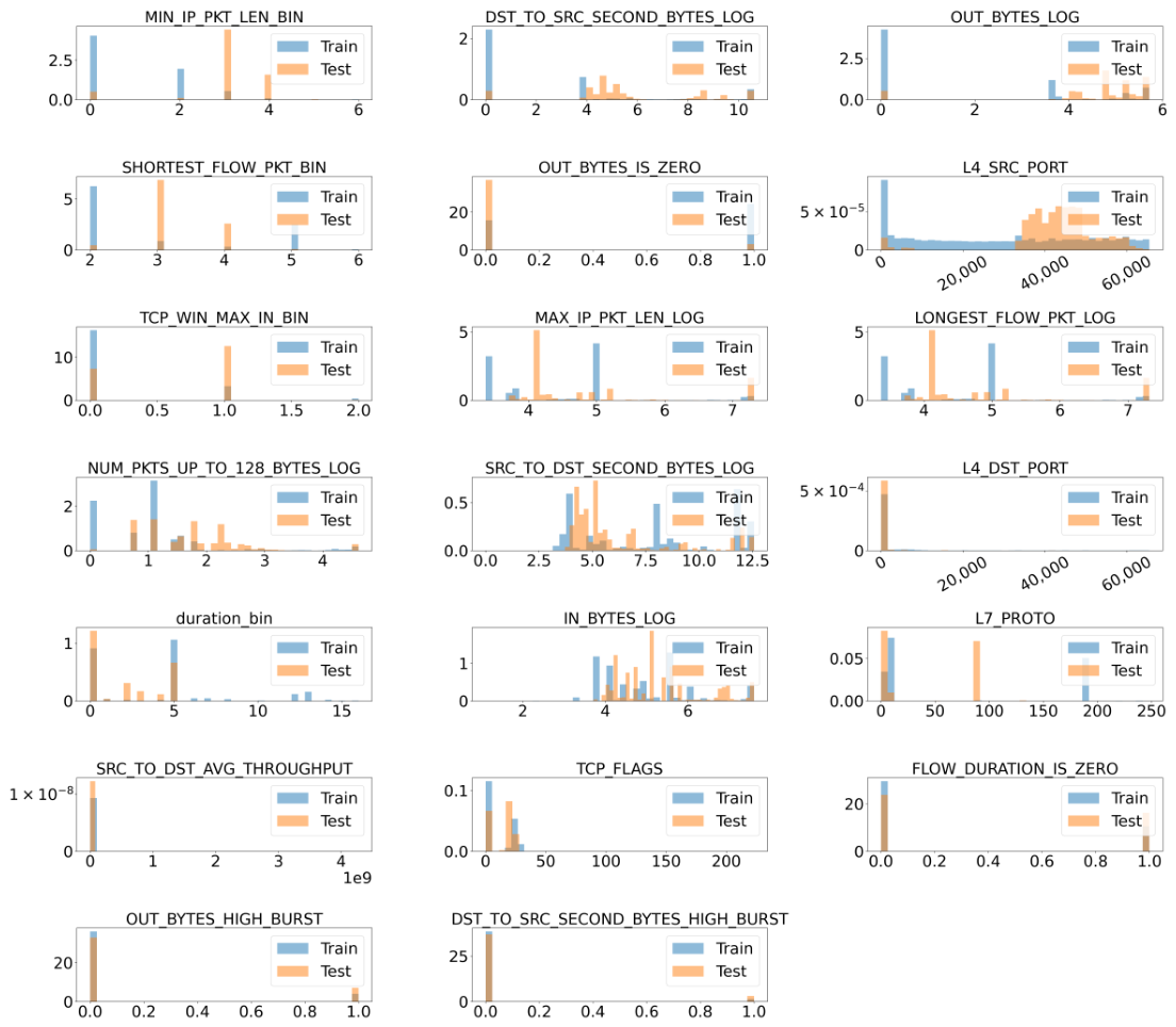
In Figure 3, where the model is trained on BoT-IoT and UNSW-NB15 and tested on ToN-IoT, the drift appears even more pronounced for several features.

Notably, SRC_TO_DST_SECOND_BYTES_LOG and DST_TO_SRC_SECOND_BYTES_LOG exhibit strong separation between training and test distributions, with minimal overlap, indicating a substantial change in traffic intensity patterns across datasets. Similarly, NUM_PKTS_UP_TO_128_BYTES_LOG and IN_BYTES_LOG demonstrate shifts toward higher values in the test set, suggesting that ToN-IoT contains systematically different packet-size and byte-volume characteristics [60].

Packet-level features further reinforce this observation. MIN_IP_PKT_LEN_BIN and SHORTEST_FLOW_PKT_BIN show pronounced distributional shifts, where the training distribution is concentrated in lower bins while the test distribution extends toward higher bins, reflecting fundamentally different minimum packet-size behaviours between the two environments. This behaviour is consistent with packet-size distribution studies, which report that traffic tends to concentrate around small control segments while showing a second mode near the maximum transmission unit (MTU) boundary [61,62,63]. Similarly, TCP_WIN_MAX_IN_BIN reveals a shift in TCP window size patterns, pointing to protocol-level differences in device and connection behaviour.

Binary-derived features such as OUT_BYTES_IS_ZERO and FLOW_DURATION_IS_ZERO also demonstrate clear discrepancies in probability mass distribution, indicating that even fundamental traffic presence patterns differ across datasets. Protocol-level features including L7_PROTO and TCP_FLAGS exhibit shifts in dominant categories, further highlighting inconsistencies in application-layer behaviour, such as those arising from differences in protocol handshakes and session-establishment patterns [64].

Port-based features such as L4_SRC_PORT and L4_DST_PORT also show clear discrepancies, where the training distributions tend to be more uniform while the test distribution introduces peaks in previously underrepresented regions, indicating differences in service usage and communication patterns. Furthermore, duration_bin exhibits a shift toward higher bins in the test set, implying longer flow durations in ToN-IoT compared to the training data.

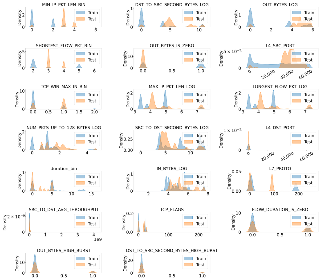
In addition to histogram-based analysis, KDE plots provide a smoother and more continuous perspective on distributional differences, enabling a more precise examination of drift patterns. Figure 4 presents the KDE-based analysis for the BoT+UNSW training and ToN-IoT test configuration, revealing distributional differences that extend beyond location shifts to fundamental changes in distributional shape.

DST_TO_SRC_SECOND_BYTES_LOG and SRC_TO_DST_SECOND_BYTES_LOG show near-complete separation between the training and test density curves, with negligible overlapping mass. This indicates that traffic intensity patterns in ToN-IoT are structurally incompatible with those observed during training, rather than merely shifted in location.

A qualitative change in modality is also evident. MIN_IP_PKT_LEN_BIN and SHORTEST_FLOW_PKT_BIN exhibit unimodal training distributions, whereas the corresponding test distributions are multimodal, suggesting that ToN-IoT captures multiple distinct packet-size regimes that are absent in the training data.

Conversely, MAX_IP_PKT_LEN_LOG and LONGEST_FLOW_PKT_LOG show the opposite pattern: bimodal training distributions that collapse into a single concentrated mode in the test set, implying reduced packet-size diversity in the test environment.

Binary features exhibit asymmetric variations in mass density. For the OUT_BYTES_IS_ZERO feature, the training distribution demonstrates a substantially higher concentration at value one compared to the test distribution. This indicates that flows with zero outgoing bytes are notably more frequent in the training environment, whereas the test environment contains a higher proportion of flows with active data transmission. A similar asymmetry appears in FLOW_DURATION_IS_ZERO, further suggesting that fundamental traffic presence patterns vary systematically across datasets.

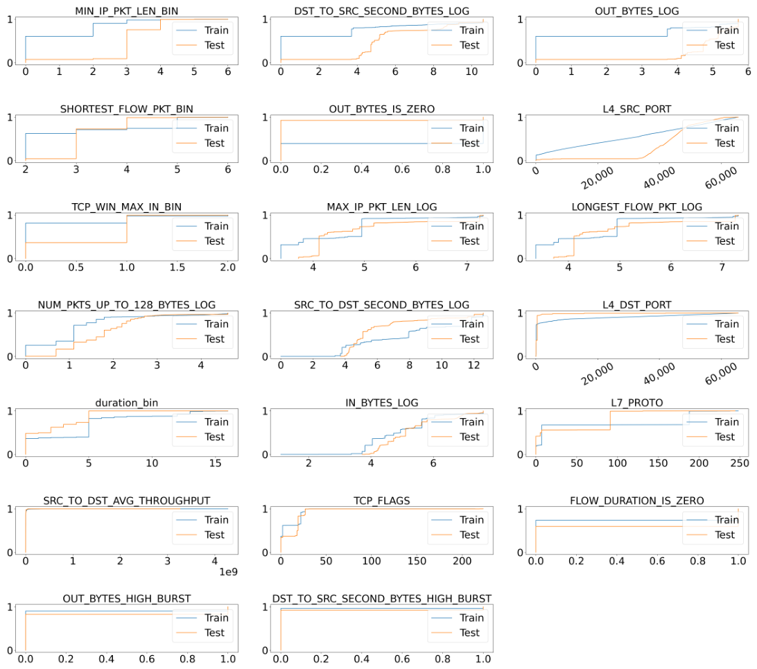
Following the KDE-based analysis, ECDF plots provide a complementary and more statistically grounded perspective on distributional shift by capturing cumulative behaviour across the entire support. Unlike histogram and KDE representations, ECDF curves allow direct observation of distributional dominance, stochastic ordering, and maximum deviation between the training and test sets.

In Figure 5, where the model is trained on BoT-IoT and UNSW-NB15 and tested on ToN-IoT, the ECDF curves show strong distributional shifts.

For SRC_TO_DST_SECOND_BYTES_LOG and DST_TO_SRC_SECOND_BYTES_LOG, the training ECDF consistently dominates the test ECDF across the entire support, with the test curve lagging substantially behind. This indicates that larger traffic intensity values are systematically more prevalent in the test domain, reflecting a clear stochastic ordering between datasets. A similar pattern appears in MIN_IP_PKT_LEN_BIN and SHORTEST_FLOW_PKT_BIN, where the training ECDF reaches its plateau at substantially lower values than the test ECDF, confirming that the test distribution is concentrated in higher bins.

In contrast, TCP_WIN_MAX_IN_BIN exhibits crossing ECDF curves, where neither distribution stochastically dominates the other. The training ECDF rises sharply at lower bin values, while the test ECDF surpasses it at higher bins, indicating a reversal in distributional ordering that cannot be characterised as a simple location shift.

Discrete binary features reveal differences in step structure rather than location. OUT_BYTES_IS_ZERO and FLOW_DURATION_IS_ZERO show substantially different jump heights at the same discrete values, with the training ECDF accumulating a larger probability mass at value zero than the test ECDF. This indicates that event frequencies for these binary indicators differ systematically across datasets. L4_DST_PORT further illustrates this asymmetry, with the training ECDF rising sharply near zero while the test ECDF increases gradually across the full port range, reflecting fundamentally different destination port usage patterns.

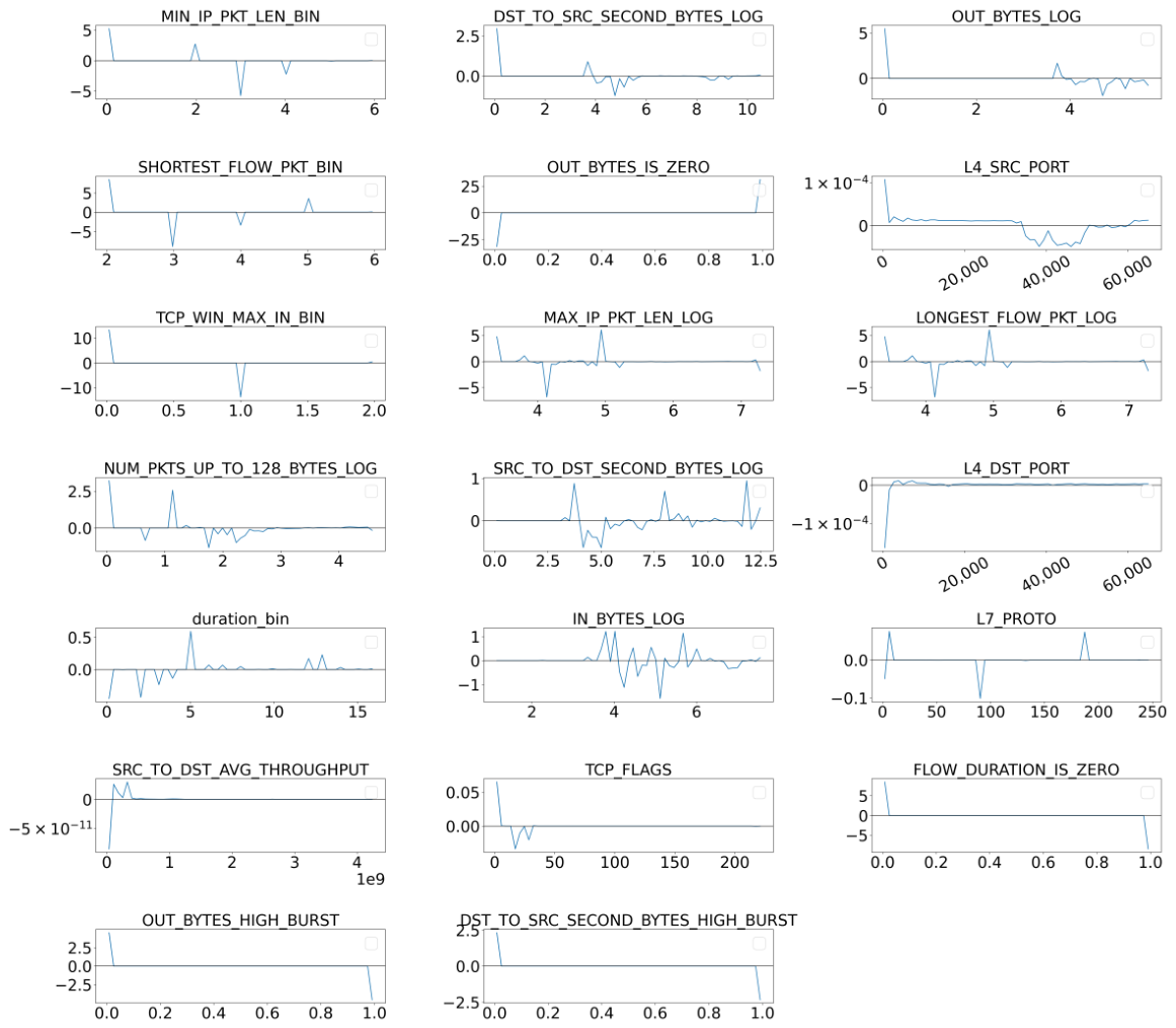
As a final step of the visual drift analysis, density difference plots provide a direct and localised quantification of distributional discrepancies by explicitly modelling the difference between training and test density functions.

Figure 6 shows the density difference analysis for the BoT+UNSW training and ToN-IoT test configuration. This representation directly quantifies the signed local discrepancy between distributions, identifying both the direction and the spatial extent of drift at each feature value.

Binary features show the largest absolute deviations. OUT_BYTES_IS_ZERO and FLOW_DURATION_IS_ZERO display sharp positive spikes at value zero and large negative spikes at value one, with peak discrepancies reaching approximately 25 units. This quantitative divergence indicates that the training distribution exhibits a predominant concentration at value zero, while the test distribution is more heavily weighted toward value one, revealing a systematic inversion of binary traffic states across datasets. A similar sign reversal appears in TCP_WIN_MAX_IN_BIN, where the positive deviation at lower bins and the negative deviation at higher bins directly corroborate the crossing ECDF pattern observed previously.

Packet-level features such as MIN_IP_PKT_LEN_BIN and SHORTEST_FLOW_PKT_BIN show clean sign transitions from positive to negative as the bin values increase, confirming that training data dominates at lower packet-size categories while the test distribution dominates at higher ones. In contrast, SRC_TO_DST_SECOND_BYTES_LOG and IN_BYTES_LOG exhibit oscillatory difference patterns with multiple sign changes, indicating that the distributional mismatch is not a simple directional shift but involves complex local density variations across the feature range.

Finally, OUT_BYTES_HIGH_BURST and DST_TO_SRC_SECOND_BYTES_HIGH_BURST show near-zero differences across most of their range, with sharp deviations only at boundary values, suggesting that drift for these features is highly localised rather than global. This pattern contrasts with the broader deviations observed in byte-volume and packet-size features, illustrating that distributional shift manifests differently depending on feature type and construction.

Across all four complementary visualisation techniques, a consistent and multi-dimensional picture of distributional shift emerges. Histogram analysis reveals shifts in the concentration regions and dominant value ranges of features, while KDE plots expose qualitative changes in distributional shape, including transitions between unimodal and multimodal structures. ECDF curves quantify cumulative ordering relationships and identify features where neither distribution stochastically dominates the other. Density difference plots further localise these discrepancies, distinguishing between global directional shifts, sign-reversing transitions, and boundary-concentrated deviations.

Critically, the observed drift is neither uniform nor restricted to a single feature category. Byte-volume features, packet-size indicators, binary traffic presence flags, TCP protocol attributes, and port-based features all exhibit distributional mismatches, albeit of different types and magnitudes. This heterogeneity implies that no single preprocessing transformation can fully resolve the cross-dataset inconsistency, and that distributional shift will manifest as a persistent challenge during model evaluation regardless of the feature engineering applied.

These findings directly motivate the experimental evaluation presented in the following section. If the feature distributions learned during training do not reflect those encountered at test time, the decision boundaries formed by machine learning models are expected to degrade in a predictable but dataset-dependent manner. The extent and nature of this degradation under different training configurations are explored in the following section.

3. Results

In this section, we evaluate the impact of drift–shift (Section 2.5) on the feasibility of constructing a reliable global IDS. The three dataset combinations introduced in Section 2.5.2 are systematically analysed using both classical machine learning and neural network models. This enables a comprehensive analysis of how distributional mismatches affect model performance across heterogeneous training and testing scenarios.

3.1. Experimental Results for Traditional Machine Learning

To evaluate the impact of distributional shift on model performance in a global IDS setting, results obtained from different dataset combinations are assessed using training ROC–AUC, test ROC–AUC, precision, recall, and F1-score metrics. The train–test ROC–AUC gap is used as a primary indicator of robustness to distributional shift, while class-wise precision, recall, and F1-scores provide insights into misclassification patterns under cross-dataset conditions.

For classification, the Extremely Randomized Trees (Extra Trees) algorithm is employed [65]. This method is well suited for heterogeneous and noisy data due to its randomised splitting strategy, where both the feature and split thresholds are selected at random. This reduces variance, improves computational efficiency, and often enhances generalisation performance.

All experiments were conducted using the ExtraTrees implementation provided by the scikit-learn library [66]. During training, 10-fold cross-validation was applied on the training set to ensure robust performance estimation. The hyperparameter space used for model optimisation is summarised in

Table 6. Hyperparameter search space for the ExtraTrees model.

Hyperparameter	Description	Range/Values
n_estimators	Number of trees in the ensemble, controlling variance reduction.	300–700
max_depth	Maximum depth of individual trees to limit model complexity.	3–7
min_samples_split	Minimum samples required to split an internal node.	30–150
min_samples_leaf	Minimum samples required at a leaf node to maintain statistical stability.	20–80
max_features	Method for selecting features at each split.	log2, sqrt
random_state	Random seed controlling stochastic elements of model construction.	0, 1, 42, 128

.

To facilitate a clearer interpretation of the cross-dataset results, we adopted a defined benchmark for distinguishing usable from unusable outcomes at the configuration level. Given the challenging nature of cross-dataset generalisation, we selected relaxed thresholds to identify configurations that retain minimal predictive utility under distributional shift.

A configuration is categorised as a suboptimal outcome when the test-set F1-score for the attack class reaches at least 0.50, with both precision and recall remaining above 0.40. This threshold identifies configurations that retain only minimal predictive utility under distributional shift, producing balanced predictions rather than collapsing toward a single class. It is important to note that an F1-score of $0.50$ is inherently insufficient for real-world operational environments. However, this relaxed threshold was established specifically as an analytical baseline to identify configurations that preserve a non-trivial predictive signal despite severe cross-dataset drift. Conversely, configurations that recover the attack class (recall ≥ 0.50) but fail to maintain precision above 0.40 are classified as impaired outcomes. These reflect broad, less selective decision boundaries where the model identifies attack instances at the cost of a high false positive rate, rather than achieving reliable, balanced detection.

Configurations exhibiting a large discrepancy between training and testing performance (e.g., an F1-score gap ≥ 0.15) are explicitly identified as overfitting cases. Configurations that satisfy neither criterion are treated as total failure outcomes within the context of the current pipeline; however, these remain instructive for analysing model behaviour under severe distributional mismatch. To characterise specific patterns of performance degradation without implying successful generalisation, suboptimal and impaired configurations are denoted by † and ‡ markers in

Table 7. Traditional ML performance under dataset drift for different attack scenarios.

Train	Test	Case	Precision	Recall	F1-Score	ROC-AUC Score (Train/Test)
BoT-IoT	ToN-IoT	Benign DoS	$0.727\pm 0.000$	$0.987\pm 0.001$	$0.837\pm 0.000$	Train: $1.000\pm 0.000$
			$0.000\pm 0.001$	$0.000\pm 0.000$	$0.000\pm 0.000$	Test: $0.046\pm 0.005$
BoT-IoT	UNSW-NB15		$0.914\pm 0.000$	$0.995\pm 0.000$	$0.953\pm 0.000$	Train: $1.000\pm 0.000$
			$0.183\pm 0.055$	$0.013\pm 0.005$	$0.023\pm 0.009$	Test: $0.884\pm 0.017$
ToN-IoT	UNSW-NB15		$0.914\pm 0.001$	$0.995\pm 0.000$	$0.953\pm 0.000$	Train: $0.992\pm 0.000$
			$0.179\pm 0.003$	$0.011\pm 0.002$	$0.021\pm 0.002$	Test: $0.216\pm 0.008$
BoT+ToN	UNSW-NB15		$0.913\pm 0.000$	$0.995\pm 0.000$	$0.953\pm 0.000$	Train: $0.999\pm 0.000$
			$0.035\pm 0.001$	$0.002\pm 0.000$	$0.003\pm 0.000$	Test: $0.547\pm 0.043$
BoT+UNSW	ToN-IoT		$0.726\pm 0.000$	$0.982\pm 0.000$	$0.835\pm 0.000$	Train: $1.000\pm 0.000$
			$0.015\pm 0.005$	$0.001\pm 0.000$	$0.001\pm 0.000$	Test: $0.177\pm 0.025$
ToN+UNSW	BoT-IoT		$0.130\pm 0.001$	$0.253\pm 0.002$	$0.172\pm 0.001$	Train: $0.993\pm 0.000$
			$0.000\pm 0.001$	$0.000\pm 0.000$	$0.000\pm 0.000$	Test: $0.029\pm 0.002$
BoT-IoT	ToN-IoT	Benign DDoS	$0.302\pm 0.000$	$1.000\pm 0.000$	$0.464\pm 0.000$	Train: $1.000\pm 0.000$
			$0.069\pm 0.082$	$0.000\pm 0.000$	$0.000\pm 0.000$	Test: $0.847\pm 0.022$
ToN-IoT †	BoT-IoT		$0.538\pm 0.020$	$0.647\pm 0.030$	$0.588\pm 0.025$	Train: $0.999\pm 0.000$
			$0.764\pm 0.020$	$0.674\pm 0.030$	$0.716\pm 0.025$	Test: $0.718\pm 0.054$
BoT+UNSW	ToN-IoT		$0.302\pm 0.000$	$1.000\pm 0.000$	$0.464\pm 0.000$	Train: $1.000\pm 0.000$
			$0.250\pm 0.433$	$0.000\pm 0.000$	$0.000\pm 0.000$	Test: $0.699\pm 0.026$
ToN+UNSW	BoT-IoT		$0.176\pm 0.002$	$0.296\pm 0.003$	$0.221\pm 0.002$	Train: $0.999\pm 0.000$
			$0.307\pm 0.010$	$0.184\pm 0.010$	$0.230\pm 0.010$	Test: $0.281\pm 0.026$
BoT-IoT	ToN-IoT	Benign DDoS–DoS	$0.270\pm 0.000$	$0.990\pm 0.001$	$0.424\pm 0.001$	Train: $1.000\pm 0.000$
			$0.363\pm 0.075$	$0.002\pm 0.000$	$0.004\pm 0.001$	Test: $0.722\pm 0.015$
ToN-IoT	BoT-IoT		$0.201\pm 0.002$	$0.626\pm 0.003$	$0.304\pm 0.002$	Train: $0.998\pm 0.000$
			$0.707\pm 0.005$	$0.266\pm 0.003$	$0.387\pm 0.004$	Test: $0.345\pm 0.006$
BoT+UNSW	ToN-IoT		$0.269\pm 0.000$	$0.985\pm 0.001$	$0.422\pm 0.000$	Train: $1.000\pm 0.000$
			$0.290\pm 0.014$	$0.002\pm 0.000$	$0.005\pm 0.000$	Test: $0.684\pm 0.019$
ToN+UNSW	BoT-IoT		$0.091\pm 0.001$	$0.214\pm 0.002$	$0.128\pm 0.001$	Train: $0.997\pm 0.000$
			$0.613\pm 0.005$	$0.368\pm 0.005$	$0.460\pm 0.005$	Test: $0.131\pm 0.005$
BoT-IoT ‡	ToN-IoT	Benign Reconnaissance	$0.985\pm 0.000$	$0.881\pm 0.028$	$0.930\pm 0.015$	Train: $0.990\pm 0.000$
			$0.162\pm 0.041$	$0.626\pm 0.000$	$0.255\pm 0.049$	Test: $0.913\pm 0.002$
BoT-IoT ‡	UNSW-NB15		$0.654\pm 0.003$	$0.194\pm 0.003$	$0.299\pm 0.003$	Train: $0.990\pm 0.000$
			$0.117\pm 0.003$	$0.508\pm 0.003$	$0.190\pm 0.003$	Test: $0.251\pm 0.006$
ToN-IoT	UNSW-NB15		$0.825\pm 0.002$	$0.981\pm 0.001$	$0.896\pm 0.001$	Train: $0.999\pm 0.000$
			$0.039\pm 0.002$	$0.004\pm 0.001$	$0.007\pm 0.001$	Test: $0.286\pm 0.023$
BoT+ToN ‡	UNSW-NB15		$0.765\pm 0.034$	$0.344\pm 0.058$	$0.473\pm 0.063$	Train: $0.995\pm 0.001$
			$0.140\pm 0.010$	$0.507\pm 0.000$	$0.219\pm 0.012$	Test: $0.368\pm 0.004$
BoT+UNSW ‡	ToN-IoT		$0.998\pm 0.001$	$0.908\pm 0.002$	$0.951\pm 0.001$	Train: $0.991\pm 0.001$
			$0.264\pm 0.003$	$0.949\pm 0.001$	$0.413\pm 0.003$	Test: $0.955\pm 0.004$
ToN+UNSW ‡	BoT-IoT		$0.634\pm 0.003$	$0.133\pm 0.003$	$0.220\pm 0.003$	Train: $0.998\pm 0.000$
			$0.308\pm 0.005$	$0.835\pm 0.005$	$0.450\pm 0.005$	Test: $0.756\pm 0.007$

Values are reported as the mean ± standard deviation across four independent runs with random seeds {0, 1, 42, 128}. Configurations marked with † (suboptimal) and ‡ (impaired) represent specific failure modes driven by dataset drift. The ‡ marker identifies cases where the model maintains high recall but suffers from low precision, while † indicates a partial breakdown of decision boundaries. Unmarked rows correspond to failure outcomes under the defined performance criteria.

, respectively.

Upon examining the model results, we observed that in the Benign vs. DoS scenario, the model trained on the combined BoT-IoT and ToN-IoT datasets achieves a training ROC-AUC score of 0.999 and a test ROC-AUC score of 0.989. However, the recall for the DoS class is limited to 0.002, with a corresponding F1-score of 0.003, which demonstrates that nearly all DoS samples are misclassified as benign traffic. Similarly, in the BoT+UNSW trained model, the test ROC-AUC score decreases to 0.921, yet the DoS recall remains only 0.001. In the ToN+UNSW configuration, the results become even weaker, with the test ROC-AUC score falling to 0.611 and the precision, recall, and F1-score all dropping to 0.000.

The individual dataset transfer experiments further confirm this lack of generalisation. When trained on BoT-IoT and tested on ToN-IoT, the model achieves a near-perfect training ROC-AUC score of 1.000, but the test ROC-AUC score drops sharply to 0.048, while all class-level metrics remain at 0.000. Likewise, when trained on BoT-IoT and tested on UNSW-NB15, the model reaches a test ROC-AUC score of 0.859, yet recall remains extremely low, at 0.008, resulting in an F1-score of 0.015. A similar pattern is also observed when the model is trained on ToN-IoT and evaluated on UNSW-NB15, where the test ROC-AUC score is 0.210 and recall is only 0.011. Within the present pipeline, none of the DoS configurations satisfy the suboptimal or impaired benchmarks introduced above, indicating that DoS detection does not transfer reliably under the chosen feature space and learner combination. This pattern holds for both individual and merged training configurations, even where the ROC-AUC score values appear acceptable, suggesting that DoS-related patterns in the unified NetFlow representation remain closely tied to dataset-specific characteristics rather than to transferable attack signatures.

The limitations of ROC-AUC-based evaluation become even clearer in the Benign vs. DDoS scenario. In the BoT+UNSW setting, the model achieves a training ROC-AUC score of 0.989, whereas the test ROC-AUC score drops sharply to 0.369. Despite the strong training result, the model fails to identify the DDoS class in the test set, with precision, recall, and F1-score all equal to 0.000. In the ToN+UNSW configuration, the test ROC-AUC score increases slightly to 0.455, and the DDoS recall reaches 0.184 with an F1-score of 0.230. However, the low precision value of 0.307 points to unstable predictions and a high number of false positives.

A similar pattern appears in the individual dataset transfer experiments. When the model is trained on BoT-IoT and tested on ToN-IoT, it achieves a perfect training ROC-AUC score of 1.000 and a high test ROC-AUC score of 0.876; nevertheless, the recall remains at 0.000, confirming a total functional failure to detect DDoS samples under cross-dataset conditions. In contrast, the ToN-IoT and BoT-IoT configuration emerges as the only suboptimal outcome in Table 7 under the introduced benchmark, with an attack-class precision of 0.764, recall of 0.674, and F1-score of 0.716, alongside balanced benign-class performance achieving an F1-score of 0.588. This result, although limited in scope, demonstrates that cross-dataset DDoS detection is not categorically infeasible within the present pipeline, but that its success depends on the direction of transfer and on the underlying distributional alignment between the source and target datasets. With the exception of this configuration, DDoS patterns learned from one dataset combination do not transfer reliably to another within the present pipeline.

To examine how class structure influences generalisation under distributional shift, DoS and DDoS attacks were combined into a single class and evaluated under cross-dataset conditions. However, this modification does not mitigate the impact of distributional shift. In the BoT+UNSW setting, the model reaches a training ROC-AUC score of 0.988, while the test ROC-AUC score remains at 0.369. The recall for the merged attack class is only 0.002, resulting in an F1-score of 0.004 and showing that the model still fails to detect attacks in a reliable way. In the ToN+UNSW configuration, the test ROC-AUC score rises to 0.455, and recall increases to 0.368, with an F1-score of 0.460. Despite this result, it remains insufficient for dependable intrusion detection.

The same instability is observed in the individual dataset transfer results. For example, when trained on BoT-IoT and tested on ToN-IoT, the model again shows an almost-zero recall value (0.002) despite a perfect training ROC-AUC score. In contrast, training on ToN-IoT and testing on BoT-IoT leads to a higher recall of 0.266, but the results still point to inconsistent decision boundaries. Under the present pipeline, none of the merged DoS+DDoS configurations satisfy the suboptimal or impaired benchmarks introduced earlier, indicating that the additional within-class variability introduced by merging exceeds what the chosen feature representation can absorb without dataset-specific overfitting. This outcome does not preclude the use of merged attack categories in cross-dataset settings; rather, it suggests that achieving balanced detection in this scenario would require feature representations or learning strategies explicitly designed to accommodate higher within-class heterogeneity.

The Benign vs. Reconnaissance scenario yields comparatively better results; however, it demonstrates clear weaknesses in cross-dataset generalisation. In the BoT+ToN setting, the large gap between the training ROC-AUC score of 0.989 and the test ROC-AUC score of 0.455 reflects poor transferability. Although recall reaches 0.507, the very low precision (0.124) limits the F1-score to 0.199, indicating a high false positive rate. In contrast, the BoT+UNSW configuration achieves a higher test ROC-AUC score of 0.934, with a recall and F1-score of 0.949 and 0.413, respectively.

However, the relatively low precision suggests that predictions remain unstable. In the ToN+UNSW setting, the test ROC-AUC score decreases to 0.742, and although recall remains high at 0.835, precision falls to 0.308, again indicating unstable decision boundaries.

The individual dataset evaluations support the same conclusion. When trained on BoT-IoT and tested on ToN-IoT, the model achieves a high test ROC-AUC score of 0.914; however, precision remains low, at 0.138, limiting the F1-score to 0.227. Similarly, when evaluated on UNSW-NB15, models trained on both BoT-IoT and ToN-IoT show catastrophic performance degradation, with test ROC-AUC scores of 0.260 and 0.252, respectively, alongside very low precision. Because these values fall significantly below the 0.50 random-chance baseline, they provide quantitative evidence of pattern inversion, where the learned features become negatively correlated with the test distribution. These findings indicate that, even in relatively simpler attack scenarios, cross-dataset generalisation remains limited.

Taken together, the results across all attack scenarios show that high ROC-AUC scores do not necessarily lead to reliable attack detection under distributional shift. In many cases, the models achieve training ROC-AUC scores above 0.98, while the recall and F1-score for the attack class drop to very low levels in the test domain. This gap shows that the learned decision boundaries are closely linked to dataset-specific distributions rather than to attack patterns that generalise across datasets.

The drift analysis presented in Section 2.5 offers a structural explanation for these performance patterns. Features exhibiting severe KS drift across all configurations, such as OUT_BYTES_LOG, MIN_IP_PKT_LEN_BIN, and DST_TO_SRC_SECOND_BYTES_LOG, are precisely the byte-volume and packet-size features that encode traffic intensity patterns unique to each dataset’s collection environment.

When the model is trained on one dataset combination, the decision boundaries formed around these high-drift features become misaligned with the test distribution, resulting in the low recall values consistently observed across attack classes. Conversely, features with lower drift values, such as OUT_BYTES_HIGH_BURST and DST_TO_SRC_SECOND_BYTES_HIGH_BURST, are more stable across datasets but carry limited discriminative power on their own. This suggests that performance degradation under cross-dataset evaluation is not random but structurally tied to the features with the highest distributional divergence.

3.2. Experimental Results for Neural Network Methodology

For consistency with the evaluation framework defined in Section 3.1, the observed results are interpreted in terms of failure, impaired, and suboptimal performance patterns, based on the predefined thresholds.

Following the evaluation of traditional machine learning approaches, the same experiments were conducted using a neural network (NN) pipeline to analyse how deep models behave under high distributional shift. This design enables a direct and fair comparison between classical and neural network paradigms under identical cross-dataset conditions.

1.

A feed-forward neural network (FFNN) was selected as the primary model due to its suitability for tabular data. The architecture consists of fully connected layers, with the input layer dynamically configured based on the number of features in each dataset. Each sample is then represented as a numerical feature vector.

2.

The hidden layers employ non-linear activation functions to facilitate the learning of complex, non-linear relationships inherent in network traffic data. While these layers increase the representational capacity of the model, regularisation mechanisms are deliberately incorporated to mitigate overfitting.

3.

The output layer is structured to address a binary classification task and produces a probabilistic prediction corresponding to the probability of the positive class. This probabilistic formulation enables not only hard label predictions but also the evaluation of threshold-dependent performance metrics such as ROC-AUC score, precision, and recall.

The model parameters that we used for this experimental setup are shown in

Table 8. Architecture and training parameters of the feed-forward neural network.

Component	Description	Value
Hidden layers	Number of fully connected hidden layers.	3
Layer dimensions	Neuron counts across hidden layers.	128 → 64 → 32
Hidden activation	Non-linear activation function for hidden layers.	ReLU
Output activation	Activation function for binary classification output.	Sigmoid
Dropout	The dropout rate is reduced in the final hidden layer.	0.3 (0.15 final)
Regularisation	Techniques applied to mitigate overfitting.	BatchNorm + Dropout
Optimiser	Gradient-based parameter update algorithm.	Adam
Learning rate	Step size for parameter updates.	0.001
Loss function	Objective function for classification.	Binary cross-entropy
random_state	Controls stochastic elements for reproducibility assessment.	0, 1, 42, 128

.

The model parameters were optimised using the backpropagation algorithm, and the validation performance was continuously monitored throughout the training. In contrast to more complex architectures, this simple network design was intentionally chosen to provide a transparent and interpretable learning framework. This choice facilitates a clearer analysis of how neural network models behave under distributional shift.

For performance evaluation, in addition to loss and accuracy, the ROC-AUC score, precision, recall, and F1-score were chosen as the main evaluation criteria to provide comparable results with traditional models.

The neural network results summarised in

Table 9. DL performance under dataset drift for different attack scenarios.

Train	Test	Case	Precision	Recall	F1-Score
BoT-IoT	ToN-IoT	Benign DoS	0.728	0.991	0.839
			0.042	0.001	0.002
BoT-IoT	UNSW-NB15		0.914	0.993	0.952
			0.194	0.019	0.035
ToN-IoT	BoT-IoT		0.270	0.625	0.377
			0.000	0.000	0.000
BoT+ToN	UNSW-NB15	Benign DoS	0.914	0.982	0.947
			0.115	0.025	0.041
BoT+UNSW	ToN-IoT		0.711	0.874	0.784
			0.113	0.043	0.063
ToN+UNSW	BoT-IoT		0.276	0.645	0.387
			0.000	0.000	0.000
ToN-IoT †	BoT-IoT	Benign DDoS	0.991	0.537	0.696
			0.785	0.997	0.879
BoT+ToN	UNSW-NB15		0.955	0.949	0.952
			0.058	0.067	0.062
ToN+UNSW †	BoT-IoT		0.991	0.537	0.696
			0.785	0.997	0.879
ToN-IoT †	BoT-IoT	Benign DoS+DDoS	0.328	0.527	0.328
			0.612	0.502	0.612
ToN+UNSW †	BoT-IoT		0.207	0.429	0.279
			0.754	0.515	0.612
ToN-IoT †	BoT-IoT	Benign Recon.	0.635	0.635	0.635
			0.519	0.519	0.519
BoT+UNSW ‡	ToN-IoT		0.985	0.969	0.977
			0.393	0.572	0.466
ToN+UNSW †	BoT-IoT		0.891	0.695	0.781
			0.553	0.816	0.660

Values represent deep learning (DL) performance metrics. Configurations marked with † (suboptimal) and ‡ (impaired) identify specific failure modes resulting from distributional shift. The ‡ marker identifies cases where the model maintains recall $\ge 0.50$ but suffers from impaired precision, while † indicates a breakdown of decision boundaries where balanced detection is lost. Unmarked rows correspond to failure outcomes under the defined performance criteria.

reveal a highly heterogeneous response to distributional shift across different dataset pairings and attack scenarios. Despite the higher representational capacity of neural networks, the observed performance patterns clearly demonstrate that discrepancies between training and test data distributions remain the primary factor limiting generalisation. When both individual and combined training configurations are considered together, this limitation becomes even more evident, as performance varies substantially depending on the specific dataset pairing.

In the Benign vs. DoS scenario, the individual experiment setups already indicate weak generalisation under the defined performance criteria. For instance, in the BoT-IoT and ToN-IoT experimental configuration, the DoS class recall declines to nearly zero, resulting in a failure to identify attack instances. A similar pattern is observed when transferring from BoT-IoT to UNSW-NB15, where only a small portion of DoS instances are correctly classified. These results show that DoS-related patterns are highly dataset-specific and do not transfer reliably even in direct pairwise evaluation.

In the combined settings, the BoT+ToN model achieves strong performance for the Benign class (F1-score = 0.947), yet the DoS class recall remains very low (0.025), indicating that combining datasets does not solve the underlying generalisation problem. The BoT+UNSW configuration shows a similar pattern, while the ToN+UNSW setting leads to a complete failure in DoS detection, confirming that distribution mismatch remains the main factor shaping model behaviour.

In the Benign vs. DDoS scenario, performance varies even more across different experimental settings. In the BoT-ToN configuration, the model maintains balanced performance for the Benign class (F1-score = 0.952), yet DDoS detection remains weak (F1-score = 0.062), indicating limited transferability of the learned patterns. The BoT+UNSW configuration further shows this instability, as the model becomes heavily biased toward the Benign class, achieving perfect recall (1.000) while completely failing to identify DDoS instances. In contrast, the ToN+UNSW configuration shows strong DDoS detection (recall = 0.997, F1-score = 0.879), but this improvement occurs together with a substantial drop in Benign class performance (recall = 0.537). This pattern suggests that the model does not learn stable representations but instead shifts its decision boundaries in a way that favours one class at the expense of the other.

When DoS and DDoS attacks are merged into a single class, the results further show the difficulty caused by distributional shift. In the individual experiment settings, the merged class already shows unstable behaviour, reflecting the increased variability introduced by combining different attack types. In the BoT+UNSW configuration, the Benign class achieves high recall (0.923) but low precision (0.282), while the merged attack class remains difficult to detect (recall = 0.126, F1-score = 0.218). This result suggests that the model struggles to form a consistent decision boundary when attack distributions become more diverse.

Although the ToN+UNSW configuration gives relatively more balanced results for the merged class (F1-score = 0.612), this comes with a substantial loss in Benign class performance (F1-score = 0.279), reflecting a trade-off rather than real robustness. These findings indicate that increasing class heterogeneity strengthens the effect of distribution mismatch instead of reducing it.

In the Benign vs. Reconnaissance scenario, relatively stronger results are observed for some dataset pairings, but generalisation is still inconsistent. In the BoT-ToN experiment setting, the Reconnaissance class shows a clear imbalance, with high recall but low precision, pointing to a high false positive rate. The BoT+UNSW configuration gives relatively stable results, with high F1-scores for both Benign (0.977) and Reconnaissance (0.466), suggesting that reconnaissance-related traffic characteristics may be more similar between these datasets. However, in the BoT+ToN configuration, the Reconnaissance class again shows imbalanced behaviour, with recall higher than precision, suggesting over-generalisation under distributional differences. A similar pattern appears in the ToN+UNSW setting, where recall remains high but precision is limited, indicating that the model tends to over-predict Reconnaissance samples when evaluated on unseen distributions. These observations show that even when the detection performance appears acceptable, the underlying decision behaviour remains unstable.

Overall, the results show that better scores in some settings do not necessarily indicate robust generalisation under distributional shift. Across all evaluated scenarios, gains in recall or F1-score for some attack classes are often accompanied by clear performance losses in the other class, pointing to unstable and dataset-dependent decision boundaries. The inclusion of both individual and combined training settings further supports this conclusion, showing that neither direct cross-dataset evaluation nor dataset merging is enough to achieve consistent generalisation. Even when some dataset pairings produce relatively strong results, these outcomes do not carry over to other settings, highlighting the strong dependence of the learned patterns on dataset-specific characteristics. These findings show that distributional shift remains a fundamental challenge for cross-dataset IoT intrusion detection.

In several configurations, strong training performance is not reflected in the test results, indicating clear overfitting behaviour under distributional shift. This observation further confirms that achieving consistent performance across datasets remains highly challenging without addressing underlying distributional discrepancies.

4. Conclusions

In this study, the performance of both traditional machine learning models and neural networks was systematically evaluated under cross-dataset training and testing settings involving multiple IoT datasets, with a particular focus on the impact of distributional shift. To ensure a fair and consistent comparison, all experiments were conducted using the same classification scenarios and comparable evaluation metrics, enabling a controlled analysis of how differences between dataset distributions affect model generalisation. The results indicate that both traditional machine learning models and neural networks exhibit a noticeable sensitivity to distributional differences between training and test datasets under the evaluated experimental settings. While relatively stronger performance is observed in certain dataset pairings, these outcomes are not consistent across different configurations and tend to vary depending on the degree of similarity between the source and target distributions. This suggests that the learned decision patterns are influenced by dataset-specific characteristics, which may limit their transferability across heterogeneous environments. When considered together, the findings suggest that, within the scope of the adopted preprocessing and modelling strategies, neither traditional machine learning methods nor neural networks consistently achieve robust generalisation under cross-dataset evaluation. However, this observation does not preclude the possibility of improved performance through alternative approaches, such as advanced feature engineering, iterative feature selection, or domain adaptation techniques specifically designed to mitigate distributional mismatch. Overall, the results provide strong evidence that distributional shift is a prevalent factor across commonly used IoT intrusion detection datasets and poses a significant challenge for cross-dataset generalisation. Rather than indicating an inherent limitation of the datasets themselves, these findings highlight the importance of developing methods that explicitly account for distributional differences when designing IoT-IDS solutions intended for deployment across diverse environments. From a practical perspective, the feature-level drift analysis serves as a model-agnostic diagnostic framework for identifying the specific attributes that drive cross-dataset generalisation errors. By quantifying feature-specific instability, researchers can target high-drift attributes for distribution-aware preprocessing or unsupervised domain adaptation (UDA). Across the evaluated feature space, many features exhibit both high drift and strong within-dataset discriminative power, resulting in misalignment between the training and test environments. When such features undergo distributional shifts at test time, the learned decision boundaries may no longer correspond to meaningful attack patterns, contributing to the recall degradation observed across multiple attack classes. The development of drift-aware feature weighting or unsupervised domain adaptation (UDA) strategies specifically targeting these identified high-drift features constitutes a robust methodological pathway for enhancing cross-dataset generalisation in IoT-IDS frameworks. It is important to acknowledge that the experimental setup in this study adopts a closed-set classification assumption, where only attack classes present in at least two of the three datasets are considered during training and evaluation. While this design choice ensures label consistency and enables a controlled comparison, it does not fully capture the complexity of real-world intrusion detection scenarios. In practice, IDSs are often exposed to previously unseen attack types. Extending this work toward open-set recognition, novelty detection, and zero-shot generalisation under distributional shift represents an important direction for future research.