Research on a Fusion Path Planning Algorithm for Mobile Robots Based on Improved A* and DWA

Abstract

In mobile robot path planning, the conventional A* algorithm often suffers from redundant node expansion and excessive turning points, whereas the Dynamic Window Approach (DWA) is prone to local optima and deviations from the global path in dynamic environments. To address these issues, this paper proposes a hybrid algorithm, termed A*-GA-DWA, which combines an improved A* algorithm with a GA-optimized DWA method. In the global planning stage, a directional six-neighborhood search strategy, an obstacle-aware adaptive heuristic function, and a turning-point smoothing method are introduced to improve path quality and reduce redundant node expansion. In the local planning stage, genetic algorithm optimization is applied to the DWA evaluation weights to enhance obstacle avoidance adaptability in dynamic environments. In addition, key nodes extracted from the global path are used as sub-goals to strengthen the coordination between global guidance and local replanning. Simulation results on a 30 × 30 map with dynamic obstacles show that, compared with conventional A*-DWA, the proposed method reduces the path length by 14.07% and the navigation execution time by 45.98%; compared with M-A*-DWA, the path length and navigation execution time are further reduced by 0.32% and 21.23%, respectively. Additional experiments on a ROS-based mobile robot platform were conducted to further validate the deployability and obstacle-avoidance capability of the proposed framework. These results provide an effective solution for mobile robot path planning tasks.

1. Introduction

With the continuous advancement of automation and intelligence in modern manufacturing, automated production has become a crucial component of industrial transformation [1,2]. In this context, mobile robots [3], as typical representatives of autonomous systems, are driving the upgrading of various industries by virtue of their flexibility and adaptability in complex environments. However, the large-scale application of mobile robots still faces numerous challenges, particularly concerning path planning technology in autonomous navigation systems. Path planning is generally divided into two primary categories: global path planning and local path planning. The main methods employed for global path planning comprise the A* algorithm [4,5,6,7], Rapidly exploring Random Tree [8,9], Ant Colony Optimization [10], and Genetic Algorithm [11], whose core objective is to determine the optimal navigation route. Notable local path planning techniques consist of the Artificial Potential Field [12,13] and the Dynamic Window Approach [14], both of which demonstrate superior performance in dynamic obstacle avoidance [15] and optimizing real-time trajectories.

Among global planning methods, A*-based algorithms have been widely adopted because of their completeness and efficiency in grid environments. Existing studies have mainly focused on improving heuristic design, reducing redundant node expansion, and enhancing path smoothness. Although these improvements have achieved good results in many applications, conventional and improved A* algorithms may still suffer from redundant search, excessive turning points, and insufficient adaptability in cluttered environments. Kala et al. [16] addressed the challenge of a robot’s path planning by combining the A* algorithm with fuzzy inference. They used a fuzzy inference system (FIS) to perform low-level planning, with the results of the A* algorithm providing guidance to the FIS planning tool, ultimately enabling global planning. An improved A* algorithm was used by Wang et al. [17] to propose a method for global path planning. By weighting the heuristic information based on the target position, their approach avoids invalid cost calculations in obstacle regions during the dynamic planning process. Furthermore, they introduced a turning node backtracking strategy to ensure an optimal number of turns along the path. To reduce both search time and the number of redundant nodes, Xu et al. [18] designed an obstacle-free rectangular boundary search to replace the traditional eight-neighborhood search. In their method, the environment is explored bidirectionally from both the start and target points. This approach generates significantly fewer nodes and facilitates the identification of optimal search nodes, thereby reducing time complexity and enhancing the overall efficiency of the algorithm. The first comparison of graph-based and sampling-based algorithms for 3D path planning using drones was conducted by Zammit et al. [19]. They introduced an innovative A* ripple-reduction algorithm, a new variant of RRT, and a uniquely designed smoothing algorithm. They addressed the shortcomings of the standard A* and RRT algorithms.

The DWA method is mainly designed for local obstacle avoidance in dynamic scenarios and shows strong adaptability to real-time changes in the surrounding environment. However, to develop path planning solutions that better adapt to dynamic environments, avoid local optima traps, and improve both planning accuracy and execution efficiency, numerous scholars have focused on the efficient integration of global and local path planning methods. Berti et al. [20] proposed a new objective function incorporating the Lyapunov stability criterion, which ensures convergence to the global solution in an asymptotic sense while maintaining collision-free motion, thereby enabling a simpler, self-sufficient method. Kang et al. [21] proposed an image-based dynamic windowing method that corrects human drivers’ driving deviations by calibrating the “Human Driving Behavior (HDB)” controller; this calibration is based on a reference path that reflects the average driving trajectory under actual road conditions. Henkel et al. [22] proposed an efficient and energy-saving local path planning method. This algorithm enhances the Dynamic Window Approach by integrating a cost function that accounts for energy consumption. The energy consumption estimated during the planning phase is predicted using a dynamically learned linear regression model. Empirical results on a mobile robot platform show that energy consumption was reduced by 9.79% compared to DWA. Lai et al. [23] proposed a novel enhanced DWA. By utilizing a distance function as the weight for the target-directed coefficient, they designed an evaluation function to optimize the heading, which effectively improved the stability of mobile robots and reduced energy consumption. Luo et al. [24] proposed a combination of an Enhanced Sparrow Search Algorithm and the DWA (ESSA-DWA). This method employs tent chaotic mapping for initialization to enhance population diversity, thereby reducing the danger of premature convergence. To address the issues of insufficient safety margins and poor smoothness in the traditional DWA, Zhu et al. [25] proposed the M-A*-DWA algorithm. During the global planning phase, the A* algorithm provides guidance to actively avoid dense obstacle regions. During the local planning phase, the DWA incorporates a global guidance term and a heading weight based on distance to mitigate the issues of local minima and goal loss. However, these enhanced algorithms may face increased computational complexity in high-density environments, especially when handling multiple obstacles. This can increase the computational burden on the system and significantly prolong the search time.

Although existing hybrid A*-DWA methods have improved mobile robot path planning to some extent, several key technical problems remain insufficiently addressed. First, the global planning stage may still suffer from redundant node expansion and excessive turning structures, which reduce path quality and execution efficiency. Second, the local planning stage often relies on manually tuned DWA evaluation weights, which limits adaptability in dynamic environments. Third, in many existing fusion frameworks, the global path mainly serves as a reference, while the ability to efficiently return to the global path after local obstacle avoidance is not sufficiently emphasized. In order to resolve these challenges, this study presents an A*-GA-DWA framework with coordinated improvements in global path generation, local trajectory evaluation, and global–local coupling.

The proposed method differs from existing hybrid A*-DWA frameworks in three aspects. First, the global planning stage is not limited to a conventional A* search but is enhanced through directional six-neighborhood screening, adaptive heuristic evaluation, and turning-point smoothing to improve path quality and reduce redundancy. Second, the local planning stage is not based on fixed empirically selected DWA weights but incorporates a GA-based optimization mechanism to improve adaptability in dynamic environments. Third, instead of using the global path only as a coarse reference, the proposed framework extracts key nodes to guide segmented local planning, thus enhancing the robot’s ability to reconnect with the global path after avoiding obstacles.

The remainder of this paper is structured as follows. Section 2 reviews the related path planning methods. Section 3 presents the improved A* algorithm, the GA-based DWA improvement, and the fusion framework. Section 4 provides simulation results and comparative analysis. Section 5 concludes the paper.

2. Overview of Path Planning Algorithms

2.1. A* Algorithm

The A* algorithm is an optimal path planning method that relies on graph search, widely applied in fields such as mobile robot navigation and map routing. It integrates the optimal-path search capability of Dijkstra’s algorithm with the directional efficiency of the greedy best-first search. Its primary objective is to identify the globally optimal path while evaluating significantly fewer nodes than either of these two foundational algorithms. The evaluation function of the A* algorithm is defined as:

$$f(n)=g(n)+h(n)$$

(1)

where f(n) denotes the total evaluation cost of node n, g(n) denotes the actual accumulated cost from the start node to the current node n, and h(n) denotes the heuristic estimated cost from node n to the target node. Here, n represents an arbitrary node considered during the search process. The node with the smallest f(n) value is preferentially expanded in order to gradually approach the goal while balancing path cost and search efficiency.

The estimated value of the heuristic function h(n) plays a crucial role in the quality of the path generated during the search process. Since different environments impose different requirements on path planning, the heuristic estimate should be designed accordingly. In the standard A* algorithm, the calculation of h(n) during path search is relatively cumbersome. Therefore, to achieve more accurate and efficient estimation of the heuristic function, a distance-based function is introduced to compute h(n).

To avoid unnecessary turns and sharp bends in the planned path, the Euclidean distance is adopted to compute the heuristic distance, which serves as the estimated cost between the current node and the target node. Assuming (x₁, y₁) and (x₂, y₂) denote the coordinates of the current node and the target node in a two-dimensional Cartesian coordinate system, respectively, the heuristic cost h(n) is expressed as follows:

$$h(n)=\sqrt{{(x_1-x_2)}^2+{(y_1-y_2)}^2}$$

(2)

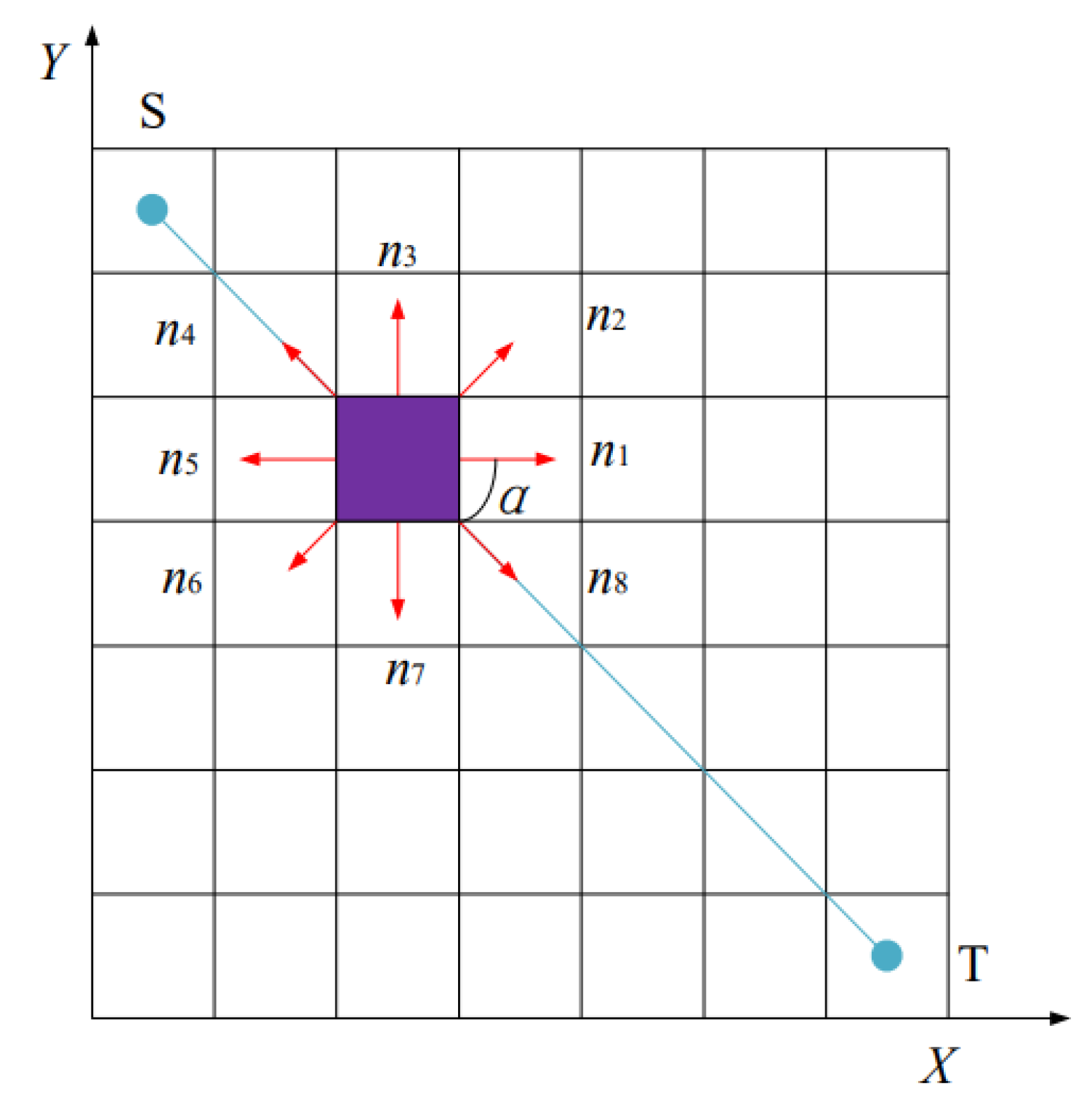
During the path search execution of the A* algorithm, it evaluates all eight feasible directions surrounding the current node, as illustrated in Figure 1. The central grid, highlighted in purple, represents the current node, and its adjacent search nodes can be denoted as follows:

$$N(i)=\left\{n_1,n_2,n_3,n_4,n_5,n_6,n_7,n_8\right\}$$

(3)

During each iteration of the path search process, all eight possible child nodes are included in the Open List. Subsequently, the algorithm evaluates the Open List and selects the node with the lowest estimated cost as the next target for expansion. Simultaneously, the current node is moved to the Closed List.

2.2. DWA Algorithm

Local path planning using the DWA primarily involves three key steps: establishing a kinematic model, sampling velocities within a feasible velocity space, and evaluating predicted trajectories.

(1)

Kinematic Modeling of the Mobile Robot

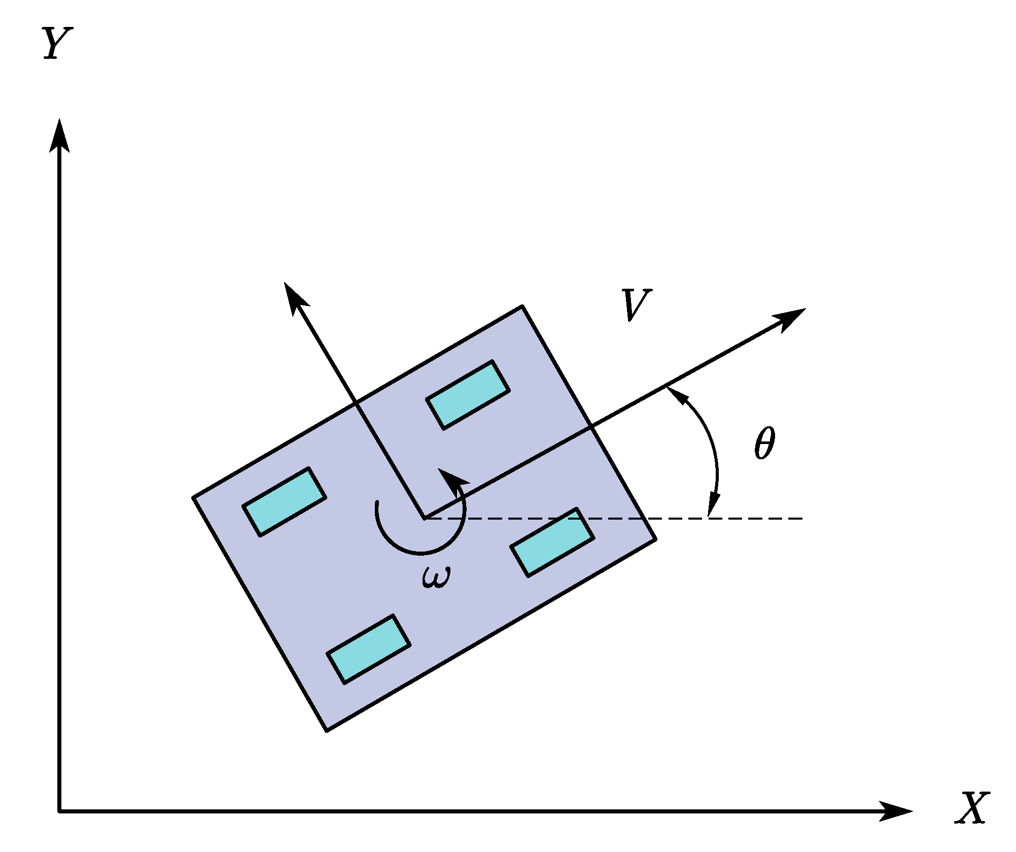
In the path planning process of the DWA algorithm, the kinematic parameters of the mobile robot must be updated, and velocity-based trajectories must be generated based on the kinematic modeling. The motion of the robot is governed by its linear velocity and angular velocity, which can be expressed as a velocity pair (v_t, w_t). The kinematic modeling of the mobile robot is illustrated in Figure 2.

During a time interval Δt, assuming the mobile robot moves by displacements Δx and Δy along the x and y directions, respectively, and the angle between its motion direction and the x-axis is Δθ. Then, the pose variation equation of the mobile robot is given as follows:

$$\left\{\begin{array}{c}\mathrm{\Delta }x=v_t\cos ({\theta }_t)\mathrm{\Delta }t\\ \mathrm{\Delta }y=v_t\sin ({\theta }_t)\mathrm{\Delta }t\end{array}\right.$$

(4)

During one control time step Δt, the robot motion is governed by its linear velocity v and angular velocity ω. The heading-angle increment is expressed as:

$$\mathrm{\Delta }\theta =\omega \mathrm{\Delta }t$$

(5)

where Δθ denotes the change in heading angle, ω denotes the angular velocity, and Δt denotes the control time step.

Based on this formulation, the pose of the mobile robot at the subsequent time step is iteratively updated.

$$\left\{\begin{array}{c}{x}_{t2}=x_{t1}+v\mathrm{\Delta }t\cos ({\theta }_{\mathrm{\Delta }t})\\ y_{t2}=y_{t1}+v\mathrm{\Delta }t\sin ({\theta }_{\mathrm{\Delta }t})\\ {\theta }_{t2}={\theta }_{t1}+\omega \mathrm{\Delta }t\end{array}\right.$$

(6)

where Δt denotes the time interval; (x_t1, y_t1) and (x_t2, y_t2) represent the x and y spatial coordinates of the mobile robot at the current and subsequent time steps, respectively; and θ_t1 and θ_t2 denote the heading angles of the robot relative to the x-axis at the current and subsequent time steps, respectively.

(2)

Velocity Sampling of the Mobile Robot

When sampling the velocity space, the mobile robot is subject to a set of hard constraints. These primarily include kinematic constraints, which set the upper and lower bounds for both linear and angular velocities; motor dynamic constraints, which establish acceleration boundaries based on motor performance and the control cycle; and collision-free constraints, which utilize real-time sensor data to calculate the minimum allowable distance between obstacles and the predicted trajectory generated by each velocity combination.

• Kinematic Constraint Space

In mobile robot motion planning, the kinematic constraint space defines the range of possible linear and angular velocities that can be achieved within a specified time interval. Specifically, the lower and upper bounds of linear velocity, denoted by v_min and v_max, determine the feasible range of linear velocity, while the lower and upper bounds of angular velocities, denoted by ω_min and ω_max, determine the feasible range of angular velocity. Accordingly, the kinematic constraint space V_s can be defined as the set of all feasible velocity pairs of the robot subject to these two constraints.

$$V_s=\{(v,\omega )| v\in [v_{\min },v_{\max }],\omega \in [{\omega }_{\min },{\omega }_{\max }]\}$$

(7)

2.

Motor Dynamic Constraint Space

The maximum output torque of the robot motor imposes an upper bound on the robot motion capability. Therefore, during trajectory simulation, the dynamic constraint space V_d can be defined according to the motor performance parameters. This constraint space includes all feasible velocities and accelerations that the robot can achieve under the motor torque limit, thereby ensuring that trajectory planning is performed within the allowable range of motor performance.

$$V_d=\{(v,\omega )| v\in [v_t-\dot{v}\mathrm{\Delta }t,v_t+\dot{v}\mathrm{\Delta }t],\omega \in [{\omega }_t-\dot{\omega }\mathrm{\Delta }t,{\omega }_t+\dot{\omega }\mathrm{\Delta }t]\}$$

(8)

3.

Collision-Free Constraint Space

During each fixed time interval, the robot receives a velocity command once. The safe velocity space V_a includes all combinations of linear velocity v and angular velocity ω that enable the robot to stop safely when necessary and thus avoid collisions with obstacles. For any velocity pair (v, ω), if the minimum distance between the simulated trajectory and the obstacles is large enough to ensure that the robot can stop in time under the limitation of the maximum motor capability, then this velocity pair is considered safe and is included in the collision-free constraint space V_a.

$$V_a=\{(v,\omega )| v\le {(2\cdot dist(v,\omega )\cdot \dot{v})}^{{\displaystyle \frac{1}{2}}}, \omega \le {(2\cdot dist(v,\omega )\cdot \dot{\omega })}^{{\displaystyle \frac{1}{2}}}\}$$

(9)

Based on the three constraint spaces described above, only the velocity combinations that simultaneously satisfy the robot’s kinematic constraints, dynamic constraints, and safety requirements are considered feasible. The intersection of these three spaces is defined as the admissible velocity set of the robot in path planning, denoted by V_r.

$$V_r=V_s\cap V_d\cap V_a$$

(10)

(3)

Trajectory Evaluation of the Mobile Robot

In the DWA algorithm, the evaluation function is crucial for determining the optimal path, as it helps select the best velocity combination that enables the robot to avoid obstacles safely while ensuring efficient movement. The evaluation function G(v, w) generally consists of the velocity evaluation term vel(v, w), the heading evaluation term head(v, w), and the collision-risk evaluation term dist(v, w). In this way, goal-directed performance, velocity optimality, and obstacle-avoidance safety are considered in an integrated manner.

$$G(v,\omega )=\alpha ·vel(v,\omega )+\beta ·head(v,\omega )+\gamma ·dist(v,\omega )$$

(11)

where α, β and γ represent the weighting parameters associated with the respective evaluation functions.

3. Fusion Algorithm Combining Improved A* and DWA

3.1. Improved A* Algorithm

In complex environments, the conventional A* algorithm suffers from node redundancy, ineffective search behavior and generated paths with excessive turning points, which are not conducive to the practical operation of mobile robots. To overcome these limitations, the A* algorithm is improved in this paper from three perspectives: the search-direction strategy, the evaluation function, and turning-point processing.

(1)

Improved Search-Direction Strategy

The conventional A* search strategy ensures that all possible neighboring child nodes are explored. However, in complex environments or environments with dense obstacles, this strategy may result in ineffective searches, thereby reducing search efficiency and increasing memory usage. To address this issue, the conventional eight-neighbor search strategy is improved in this paper according to the directional relationship between the current node and the target node. Let the current node and the target node be (x_s, y_s) and (x_t, y_t) respectively, and let the angle between the line connecting these two nodes and the positive X-axis be denoted by α.

$$\alpha =\mathrm{atan}2(y_t-y_s, x_t-x_s)$$

(12)

The planar direction is divided into eight regions N(P) with an interval of 45°. According to the interval in which α falls, only the six directional nodes aligned with or close to the target direction are retained, while the redundant node set N_r(P) is discarded. Thus, the resulting effective search node set is denoted by N_e(P).

$$N_e(P)=N(P)-N_r(P)$$

(13)

The specific relationships between the angle intervals and the retained and discarded node directions are listed in

Table 1. Relationship between the angle α and node directions

Angle α/(°)	Retained Node Directions	Discarded Node Directions
[0, 45)	n1, n2, n3, n4, n7, n8	n5, n6
[45, 90)	n1, n2, n3, n4, n5, n8	n6, n7
[90, 135)	n1, n2, n3, n4, n5, n6	n7, n8
[135, 180)	n2, n3, n4, n5, n6, n7	n1, n8
[180, 225)	n3, n4, n5, n6, n7, n8	n1, n2
[225, 270)	n1, n4, n5, n6, n7, n8	n2, n3
[270, 315)	n1, n2, n5, n6, n7, n8	n3, n4
[315, 360)	n1, n2, n3, n6, n7, n8	n4, n5

.

Therefore, the proposed method essentially pre-screens the eight-neighbor expansion nodes according to the target direction, reducing the number of candidate nodes in each expansion from eight to six. This approach effectively reduces the redundancy of nodes in the open list, minimizes the occurrence of ineffective search operations, and enhances the search efficiency of the A* algorithm in complex environments, while concurrently decreasing memory consumption. Because the retained six nodes still cover the main search region near the target direction, the proposed method can reduce redundant expansion and improve search efficiency in the tested environments. However, this strategy should be understood as an efficiency-oriented pruning mechanism rather than a strict preservation of all theoretical properties of the classical eight-neighborhood A* algorithm. Its effectiveness depends on the obstacle configuration of the environment, especially on whether a feasible path can still be found without requiring large reverse-direction detours.

In particular, the proposed six-neighborhood strategy is more suitable for environments in which the feasible path generally maintains directional consistency toward the goal. In highly cluttered maps or in scenarios requiring substantial detours, the reduced neighborhood set may weaken the search flexibility of the algorithm and may lead to suboptimal solutions. Therefore, the practical performance of this strategy should be evaluated together with the obstacle distribution of the environment.

(2)

Improvement of the Evaluation Function

In order to improve the adaptability of the conventional A* evaluation mechanism in complex environments, both the heuristic term and the actual cost term are revised in this study. The main idea is to first characterize the obstacle density between the current node and the target node, and then use this information to adaptively adjust the heuristic influence. Meanwhile, the turning complexity of the path is incorporated into the actual cost term to improve path smoothness.

To quantify the obstacle density in the current search region, the obstacle ratio P(n) is introduced and defined as follows:

$$P(n)={\displaystyle \frac{N}{(|x_s-x_t|+1)\times (|y_s-y_t|+1)}}$$

(14)

where (x_s, y_s) and (x_t, y_t) denote the coordinates of the current node and the target node, respectively, and N is the total number of obstacle grid cells in the rectangular region formed by taking these two nodes as diagonal vertices. Thus, P(n) represents the local obstacle density between the target node and the current node. A larger value of P(n) indicates a more cluttered search region and a potentially higher search difficulty.

Since the heuristic term h(n) determines the goal-directed tendency of the search process, an adaptive weighting factor related to the obstacle ratio is introduced to adjust its influence under different environmental conditions. Accordingly, the improved heuristic function is expressed as:

$$h^{\prime }(n)=e^{-P(n)}\cdot h(n)$$

(15)

where h(n) denotes the conventional heuristic cost from node $n$ to the target node, P(n) denotes the obstacle ratio defined above, and h′(n) denotes the adaptively weighted heuristic term. When P(n) is small, e^−P(n) is close to 1, and the heuristic term maintains strong goal orientation. When P(n) is large, the weighting factor decreases, thereby weakening the heuristic influence and reducing blind expansion in dense obstacle regions.

The exponential form is adopted because it provides a smooth and monotonically decreasing attenuation of the heuristic influence with respect to obstacle density. Compared with a linear penalty, the exponential weighting can preserve stronger goal-directed guidance when P(n) is small, while producing a progressively stronger suppression when the obstacle density becomes higher. In this way, abrupt changes in the search behavior can be avoided.

It should be noted that the proposed adaptive heuristic strategy is not intended to completely suppress the heuristic term. Its purpose is to reduce overly aggressive goal-directed expansion in cluttered regions. However, when the obstacle ratio becomes very high, the heuristic influence may be significantly weakened, and the search process may become more dependent on the accumulated path cost. In this case, the search behavior may partially approach a Dijkstra-like expansion. Therefore, the proposed strategy should be interpreted as an adaptive heuristic adjustment mechanism with certain environmental applicability, rather than a universally optimal heuristic design under all obstacle-density conditions.

In the conventional A* algorithm, the actual cost term mainly reflects path length and does not explicitly consider the turning complexity of the path. As a result, the generated path may contain excessive turning points. To address this problem, the number of turns from the start node to the current node is introduced into the actual cost term, and the improved actual cost is defined as:

$$g^{\prime }(n)=g(n)+M(n)$$

(16)

where g(n) denotes the conventional accumulated path cost from the start node to node n, M(n) denotes the number of turns along the path from the start node to node n, and g′(n) denotes the improved actual cost. Here, M(n) is determined according to the directional change between consecutive path segments so that paths with more turning points receive a higher actual cost. Accordingly, the improved evaluation function f′(n) can be obtained:

$$f^{\prime }(n)=g^{\prime }(n)+h^{\prime }(n)$$

(17)

In summary, in the proposed improved evaluation function, g′(n) characterizes the actual path cost, while h′(n) adaptively adjusts the influence of the heuristic function under different environmental conditions. In this way, path length, path smoothness, goal-directedness, and environmental complexity are considered in an integrated manner, thereby improving the search performance of the algorithm in complex grid environments.

Different from Weighted A*, which uses a fixed weight to strengthen the heuristic term, the proposed method adaptively adjusts the heuristic influence according to the obstacle ratio P(n). Weighted A* can improve goal-directed search efficiency in relatively open environments, but it may still guide the search too aggressively toward the target in cluttered maps. In contrast, the proposed adaptive heuristic strategy reduces the heuristic influence when the local obstacle ratio increases, thereby improving the balance between search efficiency and environmental complexity.

(3)

Turning-Point Smoothing Strategy

To mitigate the issue of excessive turning points in the path generated by the A* algorithm, resulting in unsatisfactory path quality, an improved turning-point smoothing strategy is adopted in this section. While maintaining path stability, this strategy generates a path that demonstrates improved performance in terms of both path length and the number of turns, thus offering a more dependable global path for subsequent real-time obstacle avoidance.

A turning point is defined as a point on the path where the current node, its parent node, and at least one child node are present, but these three nodes are not collinear. Based on this characteristic, the key turning points along the path can be identified. Let the coordinates of the current node be (x_i, y_i), and let the grid width be b. Then, the turning-point matrix K_i can be expressed as:

$$K_i={\displaystyle \frac{1}{b}}\left[\begin{array}{cc}{x}_i& y_i\\ x_i& y_i\end{array}\right]-\left[\begin{array}{cc}{x}_{i-1}& y_{i-1}\\ x_{i+1}& y_{i+1}\end{array}\right]$$

(18)

$$\left\{\begin{array}{l}{K}_i=0, the current node is a turning point\\ K_i\ne 0, the current node is not a turning point\end{array}\right.$$

(19)

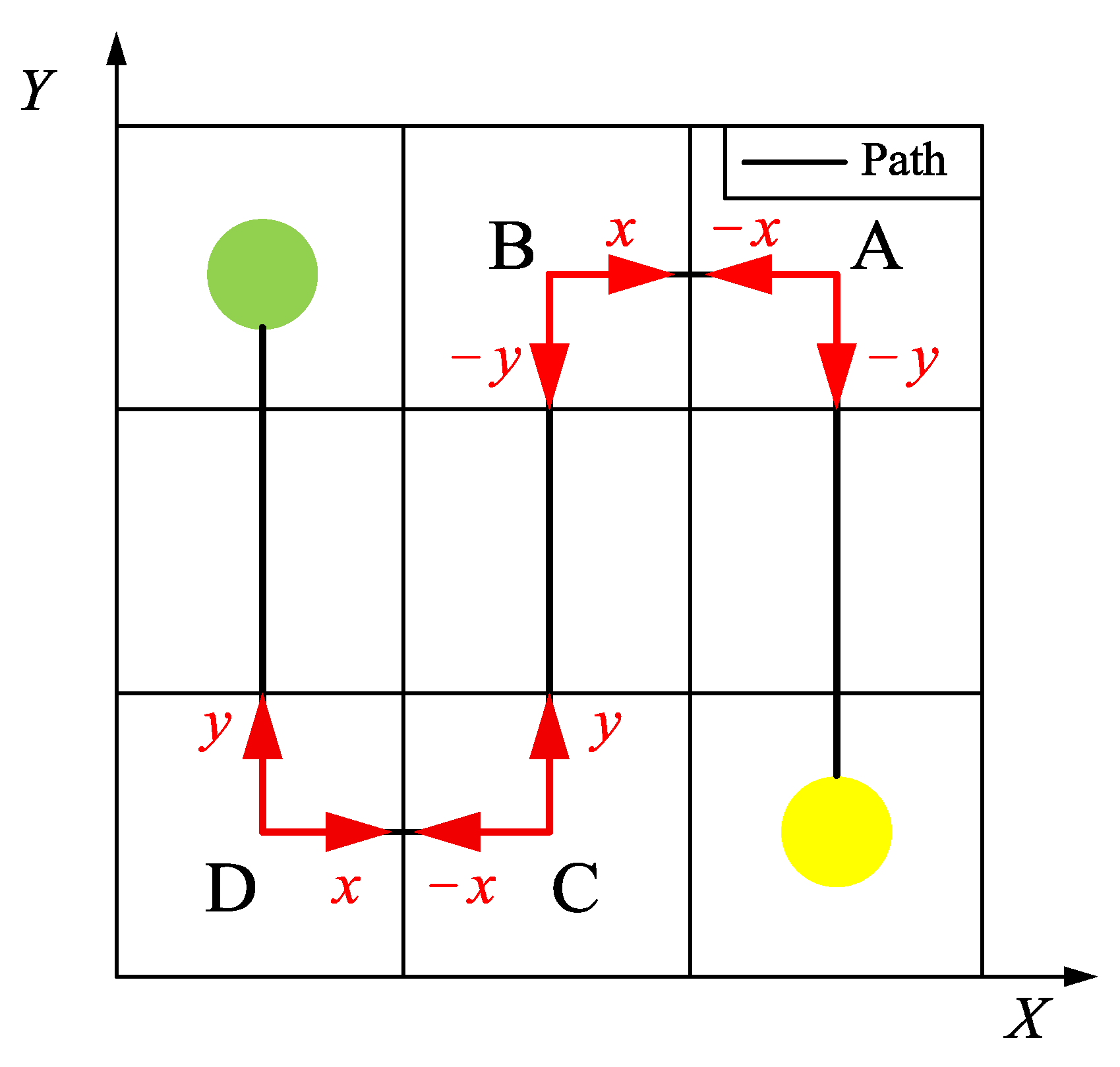
To eliminate redundant turning points, each turning point can be folded toward the turning direction. The specific procedure for this determination is shown in Figure 3.

As illustrated in Figure 3, the grid containing the yellow point denotes the start point, while the grid containing the green point denotes the target point. The line connecting these two points represents the planned path. According to the matrix P_i, the entire path contains four turning points, denoted by A, B, C and D. The turning direction of each turning point is determined by the quadrant in which the line segments connecting the turning point to its adjacent upper and lower nodes are located in the coordinate system.

Turning-point smoothing means that each turning point is folded toward its turning direction and expanded along the diagonal direction of the rectangle formed by the two adjacent nodes of the current node, so as to reduce the number of turning points. Let the current turning point be P_i, and let its folding direction vector be denoted by d_i. Then, the new node after the m-th folding operation can be expressed as:

$$P_i^{(m)}=P_i+m{d}_i$$

(20)

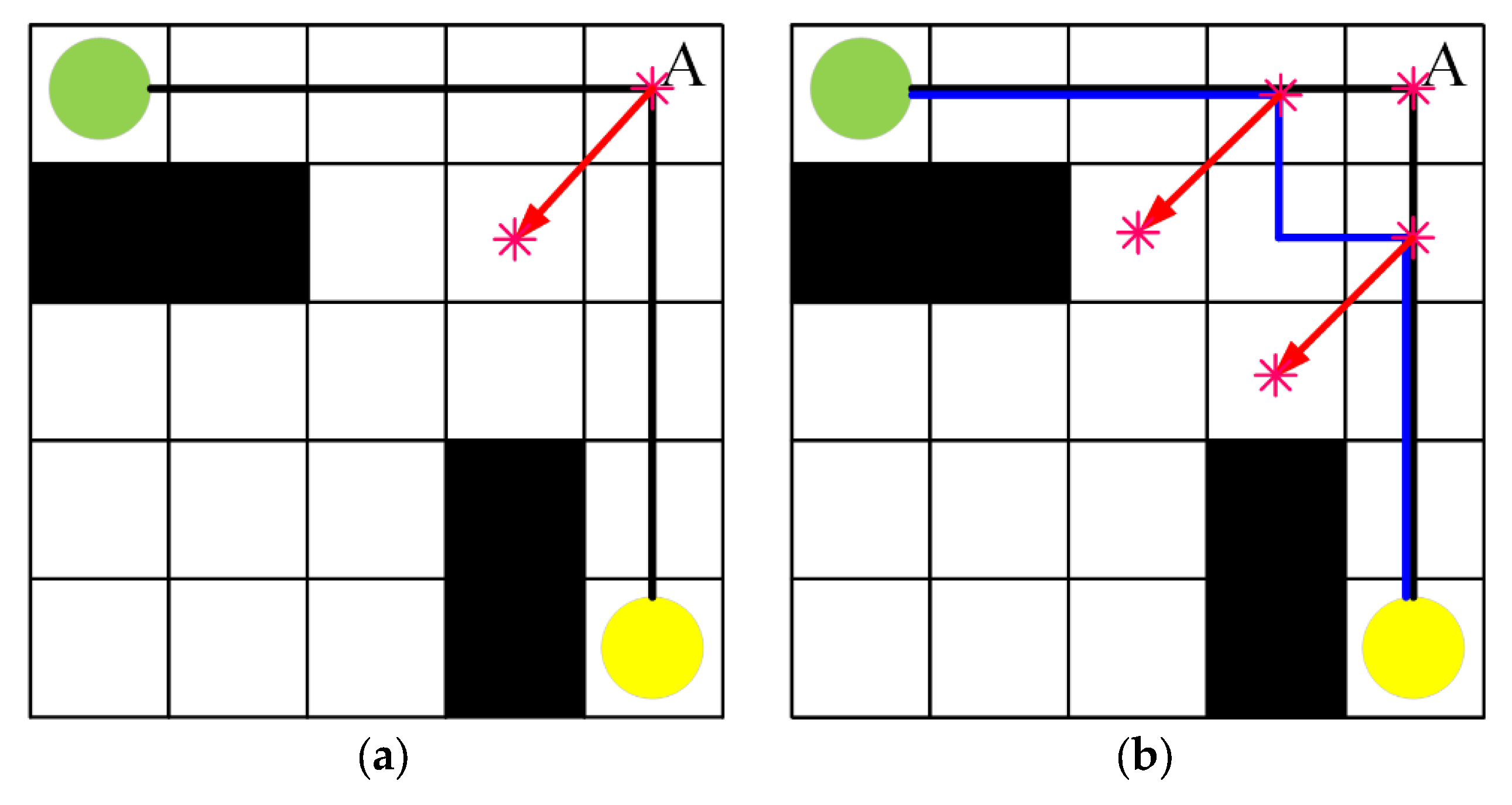
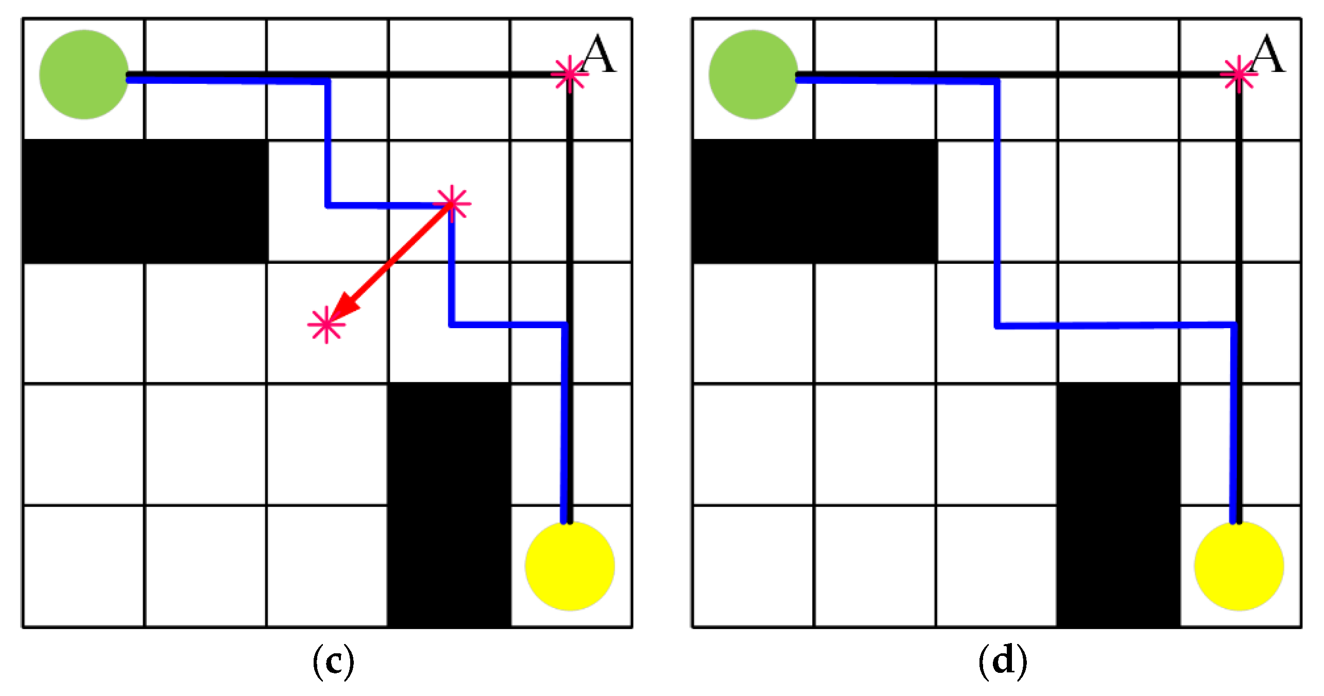
The detailed folding and expansion process is shown in Figure 4.

In Figure 4, the grid containing the yellow point denotes the start point, whereas the grid containing the green point denotes the target point. The black polyline represents the initial path, and point A is a turning point. Panels (a), (b), (c) and (d) illustrate the complete folding process of the turning point. Since the turning direction of turning point A is toward the third quadrant, the folding operation is performed in that direction. In each step, the turning point is folded by one grid cell. Each folding operation introduces a new turning point, and the newly generated turning point is then continuously folded in the same turning direction until the next folding step is blocked by an obstacle and can no longer be executed. Therefore, the termination condition of the folding process can be expressed as:

$$P_i^{(m)}\in Obs$$

(21)

where Obs denotes the set of obstacle grid cells.

The path obtained after the folding process may still contain turning points and therefore requires further smoothing. During multiple folding operations on the initial path, each folded path partially overlaps with the original path. The non-overlapping portion generated during the entire folding process is defined as the turning-point smoothing improvement region. Taking the common points of the paths after each folding operation as vertices, a rectangular region is formed, which corresponds to the turning-point smoothing improvement region. The non-overlapping portions between the folded path and the initial path form two sides of this rectangle, while the diagonal connecting the rectangle vertices constitutes the improved path after turning-point smoothing. Let the initial path be L₀, and let the folded path after improvement be L₁. Then, the final improved path L can be expressed as:

$$L=(L_0-L_c)\cup L_1$$

(22)

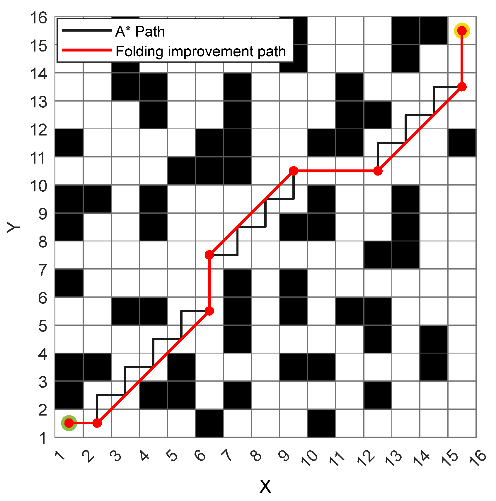
where L_c denotes the turning-point path segment in the original path. The improved path after turning-point smoothing is illustrated in Figure 5.

As shown in Figure 5, after turning-point folding and smoothing, the redundant turning points in the original path are effectively reduced. While preserving path feasibility, the improved path further decreases the number of turns and enhances path smoothness and executability.

The proposed turning-point smoothing strategy is a constrained post-processing step applied to an already feasible global path. Its purpose is not to re-search the global route, but to locally simplify the turning structure while preserving path feasibility. During the folding process, each candidate folded segment is accepted only when it does not intersect any obstacle cell. Therefore, the smoothing operation is always performed under explicit obstacle constraints, and the resulting path remains in the feasible free space of the grid map. Since only local turning segments are adjusted, the global connectivity between the start point and the goal point is not changed.

To improve reproducibility, the turning-point folding process is performed under explicit geometric and collision-free constraints. First, each candidate folded node must remain inside the valid map boundary; otherwise, the current folding process is terminated. Second, the smoothing operation is carried out on the inflated obstacle map, in which the obstacle region has been expanded according to the robot size and the required safety margin. Therefore, the feasibility check is not limited to the candidate node itself but also includes the newly generated connection segment. A candidate folded segment is accepted only when it does not intersect any inflated obstacle cell and does not cross obstacle corners in a way that would make the smoothed path infeasible.

The folding process is terminated when one of the following conditions is met:

• the next candidate folded node lies outside the map boundary;
• the candidate node intersects the inflated obstacle region;
• the newly generated segment is not collision-free;
• the smoothed segment crosses an obstacle corner and becomes infeasible;
• further folding no longer reduces the local turning structure.

Once any of these conditions is reached, the current feasible folding result is taken as the final smoothing state for the corresponding turning point. We compared several path smoothing methods, as summarized in

Table 2. Qualitative comparison of different path smoothing methods.

Method	Advantage	Limitation	Relation to This Study
B-spline smoothing	High smoothness	May cross obstacle regions if collision constraints are not added	Suitable for continuous smoothing but requires additional collision checking
Bezier curve	Simple and smooth	Curve may deviate from original grid path	May reduce sharp turns but may affect grid-map feasibility
Theta*	Produces shorter and smoother paths	Requires repeated visibility checking	Similar in reducing unnecessary turns but changes search process
Turning-Point Smoothing	Maintains grid feasibility and reduces sharp turns	Adds post-processing overhead	Designed for grid-based paths and preserves local feasibility through collision checking

.

As shown in Table 2, compared with curve-based smoothing methods such as B-spline and Bezier curves, the proposed method is more conservative because it only modifies local turning structures under explicit grid-based collision constraints. Compared with Theta* and line-of-sight smoothing, the proposed method is implemented as a post-processing strategy and does not change the main A* search process. Therefore, it is suitable for improving the geometric quality of grid-based paths while maintaining obstacle feasibility.

3.2. Improved DWA Algorithm

While the evaluation function of the DWA algorithm performs reliably in standard environments, it may encounter difficulties in complex or constrained spaces. In particular, it provides only limited safety margins when the robot moves close to obstacles. Meanwhile, the empirical setting of evaluation function parameters introduces subjectivity, which may easily cause oscillatory paths when the trajectory approaches obstacles and prevents the algorithm from dynamically balancing motion speed and obstacle-avoidance capability as a response to environmental changes. To overcome these limitations, this paper develops a DWA evaluation function improved by a genetic algorithm (GA) to enhance adaptability and safety. The main steps are as follows.

The optimization variable is the DWA evaluation-weight vector, expressed as x_i = [α_i, β_i, γ_i]. For each candidate parameter vector, the complete planning procedure is executed once, and the returned scalar planning cost is taken as the objective value. Therefore, the optimization problem is formulated as:

$$\left\{\begin{array}{l}{x}_i = \left[{\alpha }_i, {\beta }_i, {\gamma }_i\right]\\ \min F\left(x_i\right)\end{array}\right.$$

(23)

where α_i, β_i and γ_i denote the DWA evaluation weights of the $i$-th individual. For each candidate vector x_i, the corresponding DWA weights are assigned to the planner, and the complete path planning process is executed once to evaluate its performance. The objective value is defined as:

$$F(x_i)=\left\{\begin{array}{c}J(x_i), if the planning process is completed successfully\\ {10}^6, if the planning process fails\end{array}\right.$$

(24)

where J(x_i) denotes the scalar comprehensive planning cost returned by the planning program under the weight vector x_i, and 10⁶ is a large penalty value assigned to failed planning cases.

In the present implementation, a failed planning case refers to the situation in which the planning program cannot return a valid scalar cost value. In such a case, a large penalty value is directly assigned to the objective function to suppress infeasible or unsuccessful parameter combinations during the evolutionary process. Therefore, the GA optimization is carried out at the level of the complete planning-process output, rather than by separately recombining several manually defined sub-indicators in the optimization layer.

If the path planning result is better, the corresponding value of F(x_i) becomes smaller; otherwise, when planning fails or the performance is unsatisfactory, a larger penalty value is assigned. Through this objective function, the quality of the DWA weighting parameters can be converted into a comparable numerical indicator. During the genetic algorithm search process, an initial population of parameter sets is first generated randomly, and the fitness of each parameter set is then evaluated. Since the optimization objective in this study is minimization, the fitness of the $i$-th individual, denoted by f_i, can be defined as:

$$f_i = F\left(x_i\right)$$

(25)

The best individual in the current population is denoted by x_best and can be expressed as:

$$x_{best}=\underset{x_i}{\arg \min }{f}_i$$

(26)

To improve the retention probability of superior individuals, the selection operation adopts a probability assignment strategy based on the reciprocal of the fitness value, denoted by p_i.

$$p_i={\displaystyle \frac{1/(f_i+\epsilon )}{{\displaystyle \sum _{k=1}^{N}1}/(f_k+\epsilon )}}$$

(27)

where ε is a very small positive constant introduced to avoid division by zero.

Subsequently, the crossover operation is performed to recombine superior parameter sets, while the mutation operation is used to enhance population diversity and prevent the algorithm from getting trapped in a local optimum. As the iteration proceeds, the population gradually converges toward a better region, and an optimal set of weighting parameters, denoted by x′, is finally obtained:

$$x^{\prime }=[{\alpha }^{\prime },{\beta }^{\prime },{\gamma }^{\prime }]$$

(28)

By substituting x′ into the DWA evaluation function in Equation (10), the improved evaluation model G′(v, w) can be obtained:

$$G^{\prime }(v,\omega )={\alpha }^{\prime }·vel(v,\omega )+{\beta }^{\prime }·head(v,\omega )+{\gamma }^{\prime }·dist(v,\omega )$$

(29)

Compared with the conventional DWA method, which relies on repeated empirical parameter tuning, the genetic algorithm is capable of searching for a better combination of evaluation function parameters in the global search space. This reduces the blindness of parameter selection and improves the local obstacle-avoidance capability, trajectory smoothness, and operational stability of DWA in dynamic environments, thereby providing a more rational parameter basis for the efficient integration of global path planning and local planning.

In this study, the GA optimization is implemented with a population size of 20 and a maximum generation number of 30. The decision variables are the DWA evaluation weights [α, β, γ], and their lower and upper bounds are set as [0, 0, 0] and [1, 1, 1], respectively. Roulette-wheel selection based on inverse fitness is adopted, while one-point crossover and random-reset mutation are used with probabilities of 0.8 and 0.2, respectively. The optimization process is terminated when the maximum generation number is reached. The GA optimization is performed offline, and the optimized weight set is then used in the subsequent DWA-based local planning process.

The performance of the DWA algorithm is influenced not only by the evaluation function weights but also by velocity sampling resolution, prediction horizon, trajectory generation model, velocity constraints, acceleration constraints, and obstacle cost design. Therefore, the present study does not claim that weight optimization alone can fully determine the performance of DWA in all dynamic environments. Instead, the proposed GA-based strategy focuses on improving the balance among heading, obstacle clearance, and velocity evaluation under a fixed DWA configuration.

3.3. Fusion Algorithm

In practical applications, relying exclusively on global path planning may result in collisions with dynamic obstacles and unknown static obstacles within the environment, thereby increasing safety risks. By contrast, relying only on local path planning may lead to insufficient directional guidance because of the lack of global guidance. Therefore, a hybrid path planning method that combines global and local planning is required. Specifically, the global algorithm is applied to generate a global path based on known environmental information, after which the local algorithm is applied to avoid unknown and moving obstacles encountered during navigation. In this way, the mobile robot can maintain stronger directionality while performing real-time local obstacle avoidance and ultimately reach the target point successfully.

This paper presents a hybrid path planning algorithm that integrates the improved A* and DWA methods. Initially, the enhanced A* algorithm is employed for global path planning, guiding the robot along an optimal path from the starting point to the target. Next, sub-target points are set along the global path, and the DWA algorithm is employed to carry out segmented local path planning, avoid obstacles, and prevent the robot from falling into a local optimum. Finally, the performance of the DWA algorithm is further improved by introducing a genetic algorithm-based evaluation function to select the optimal path, thereby effectively enhancing the adaptability and safety of the proposed algorithm.

In this study, the key nodes are defined as the turning points extracted from the global path generated by the improved A* algorithm. A path node is regarded as a key node when the direction of the path changes at this node. Therefore, the key-node sequence preserves the main geometric structure of the global path and provides intermediate sub-goals for the DWA-based local planner. The key-node sequence can be expressed as:

$$K=\left\{k_1,k_2,\dots ,k_m\right\}$$

(30)

where K denotes the ordered key-node set, and k_j denotes the j-th turning point used as a temporary sub-goal during local planning. The final target point is also included in the sequence to ensure that the robot can eventually reach the destination.

During local planning, the DWA algorithm uses the current key node k_j as the temporary sub-goal. When the robot reaches the current key node, the next key node k_j+1 is selected as the new sub-goal. In the implementation, the switching condition is defined as:

$$\parallel p_r-k_j\parallel <d_{th}$$

(31)

where p_r denotes the current robot position, k_j denotes the current key node, and d_th denotes the distance threshold for determining whether the robot has reached the current key node. This procedure is reiterated until the final target point is reached.

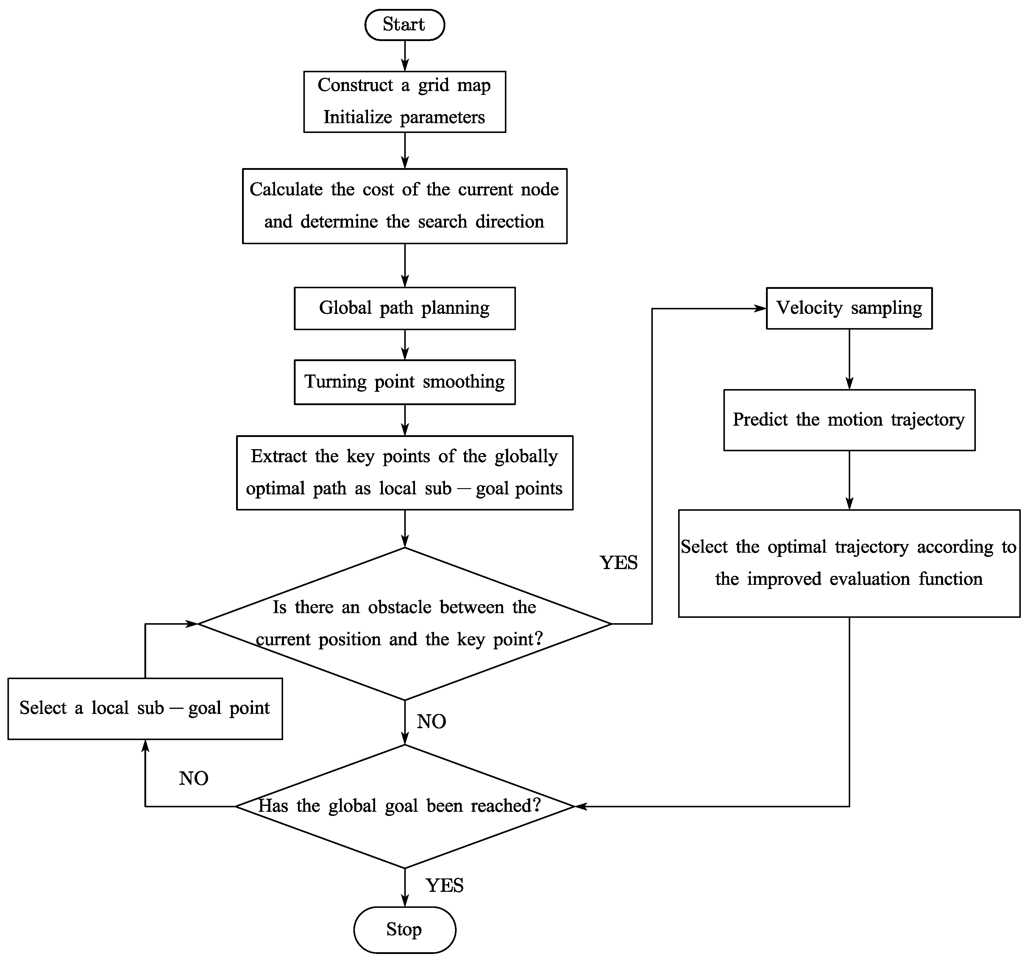
By using turning points as sub-goals, the local planner does not directly pursue the final target over a long distance. Instead, it follows the main directional structure of the global path step by step. This strategy strengthens the consistency between global planning and local obstacle avoidance, reduces unnecessary deviation after local replanning, and helps the robot return to the global path more effectively. Figure 6 illustrates the flowchart of the fusion algorithm.

The proposed A*-GA-DWA framework consists of several improvement modules, and each module contributes to the final planning performance from a different perspective. In the improved A* stage, the direction-based six-neighborhood pruning strategy mainly reduces redundant node expansion by preferentially retaining the search directions closer to the target. This module is closely related to the reduction in expanded nodes observed in the experiments. The obstacle-ratio-based adaptive heuristic weighting strategy further adjusts the influence of the heuristic function in accordance with the local obstacle distribution, which helps the algorithm balance goal-directed search and obstacle-aware expansion in complex maps. The turning-point smoothing strategy mainly improves the geometric quality of the global path by reducing sharp turns and large-angle direction changes, and it is, therefore, related to the reduction in turning angle and the enhancement of path smoothness.

In the local planning and fusion stage, the GA-based DWA weight optimization improves the selection of the evaluation function weights α, β, and γ, thereby improving the balance among heading consistency, obstacle clearance, and velocity preference during local trajectory evaluation. The key-node guidance strategy extracts turning points from the global path and uses them as intermediate sub-goals for DWA. This prevents the local planner from directly pursuing the final target over a long distance and helps the robot return to the global path after local obstacle avoidance. Therefore, the reduction in path redundancy and navigation execution time in the dynamic-obstacle scenario is attributed to the combined effect of improved global path quality, GA-optimized local evaluation, and key-node-guided global–local coordination.

In contrast to existing hybrid A*-DWA methods, which primarily integrate a global planner with a local obstacle-avoidance module in a sequential manner, the proposed A*-GA-DWA framework introduces coordinated enhancements at three interconnected levels: global path generation, local trajectory evaluation, and path recovery after obstacle avoidance. Therefore, the contribution of this paper lies not only in improving A* and DWA separately, but also in strengthening the coupling between global planning and local replanning. This enables the robot to better maintain path quality, improve adaptability in dynamic environments, and reconnect more efficiently with the global path after obstacle avoidance.

4. Simulation and Experimentation

To assess the effectiveness and performance of the proposed algorithm, simulation experiments were carried out using MATLAB R2022 (MathWorks, Natick, MA, USA) on the Windows 10 operating system. The experiments were conducted on a system equipped with an Intel Core i7-13650HX processor and 32 GB of RAM. To enhance the statistical reliability of the evaluation, each algorithm under comparison was independently executed multiple times under identical experimental conditions. Unless specified otherwise, the reported results are presented as the mean ± standard deviation from repeated trials.

4.1. Simulation Experiments of the Improved A* Algorithm

Four maps were used to compare the conventional A* algorithm with the improved A* algorithm through simulation. The comparison mainly focused on path length, search time, number of expanded nodes, and turning angle. The four map environments were 10 × 10, 30 × 30, 50 × 50 and extreme maps. Within the simulation maps, blue triangles correspond to starting positions, green circles signify target locations, black cells depict static obstacles, and gray cells illustrate the nodes traversed during path searching.

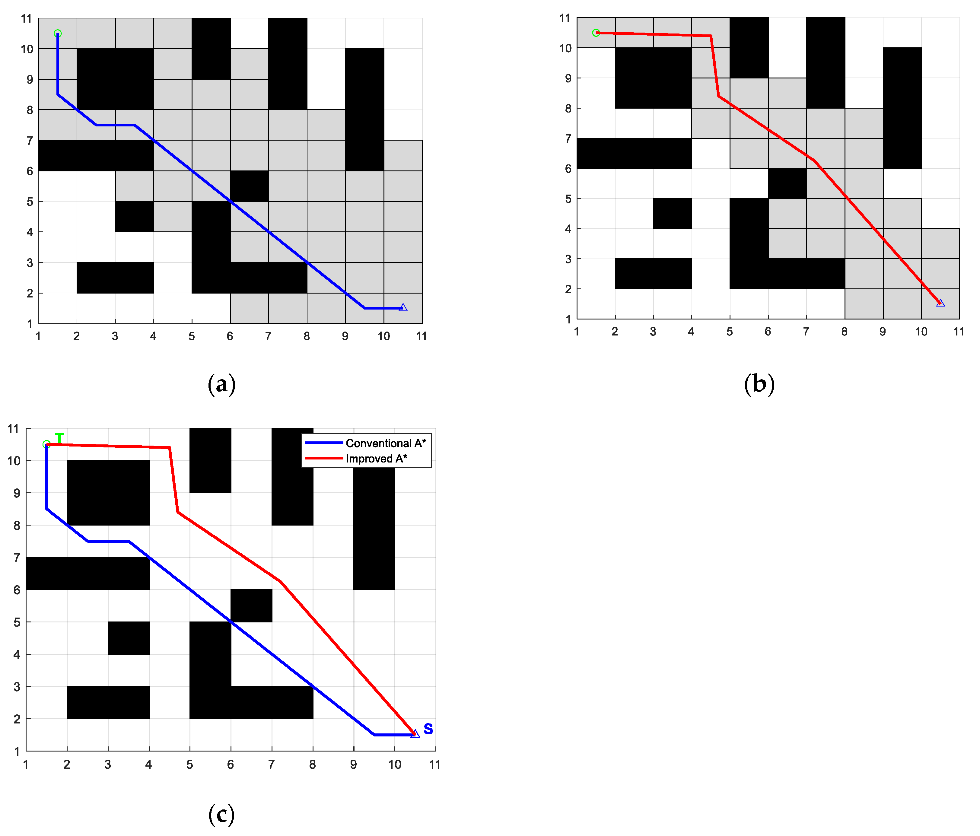
In the 10 × 10 grid, the starting point was positioned at (1, 10), the goal at (10, 1), and the obstacle coverage reached 23%. Figure 7 and

Table 3. Comparison of path parameters on the 10 × 10 map.

Map	Algorithm	Planning Time/s	Turning Angle/°	Number of Turns	Path Length/m	Number of Nodes
10 × 10	Conventional A*	0.007 ± 0.011	180	4	13.89	51
	Improved A*	0.012 ± 0.016	140.71	3	14.09	34

present the path planning results for the conventional and enhanced A* algorithms.

As illustrated in Figure 7, the path produced by the conventional A* successfully reaches the goal, yet it has a notable limitation. When planning paths across different grid maps, the generated path may pass through obstacle vertices, such as (1, 7) and (3, 10) in Figure 7a. This results in insufficient safety margins for the robot and makes collisions more likely, especially in narrow passages. On the other hand, the improved A* algorithm, through the weighted heuristic strategy and the turning-point smoothing strategy, generates a path that does not pass excessively close to obstacles. Consequently, the safety of the planned path is significantly improved, and the overall path is smoother.

As shown in Table 3, on the 10 × 10 grid map, the improved A* algorithm reduces the turning angle by 21.82%, the number of turns by 25.00%, and the number of expanded nodes by 33.33% compared with the conventional A* algorithm. These results indicate that the improved algorithm can reduce redundant search and improve path smoothness in a simple environment. However, the planning time increases by 69.54%, and the path length increases by 1.40%. This suggests that in relatively simple maps, the benefit of reducing redundant node expansion is limited, whereas the additional cost introduced by adaptive evaluation and turning-point smoothing becomes more noticeable in the total planning process. Therefore, the proposed strategy does not show a clear overall efficiency advantage in simple environments, although it still improves path smoothness and path safety.

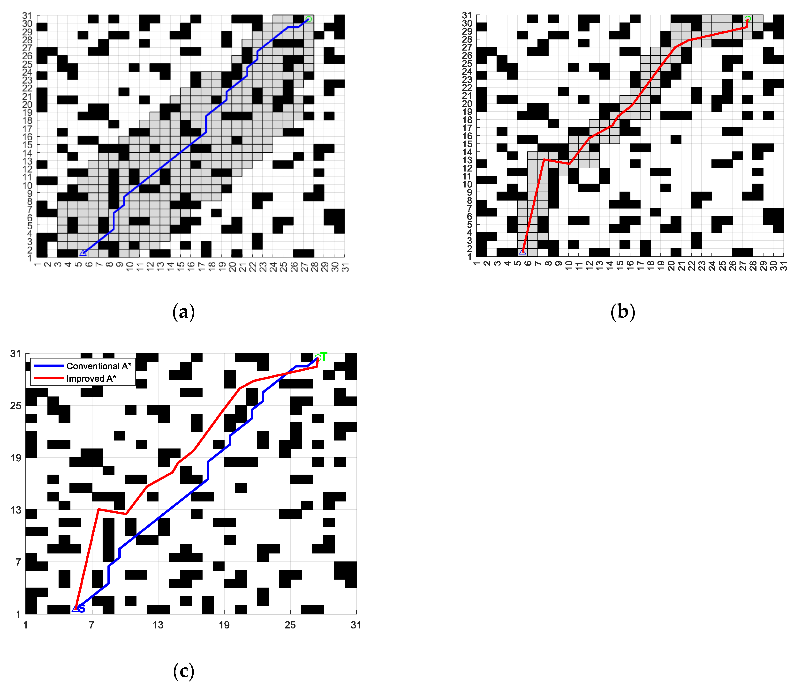
In the 30 × 30 grid map, the start point was set at (1, 5), the target point was set at (30, 27), and the obstacle coverage rate was 25%. The planning results for both the conventional A* and the improved A* are displayed in Figure 8 and

Table 4. Comparison of path parameters on the 30 × 30 map.

Map	Algorithm	Planning Time/s	Turning Angle/°	Number of Turns	Path Length/m	Number of Nodes
30 × 30	Conventional A*	0.019 ± 0.007	630	14	38.69	278
	Improved A*	0.025 ± 0.006	365.56	10	40.83	104

.

As presented in Table 4, on the 30 × 30 grid map, the improved A* algorithm reduces the turning angle by 41.97%, the number of turns by 28.57%, and the number of expanded nodes by 62.59% compared to the conventional A* algorithm. These results demonstrate that the enhanced algorithm can efficiently minimize redundant node expansions and enhance path smoothness in more complex environments. Although the planning time and path length increase by 33.09% and 5.52%, respectively, the substantial reduction in expanded nodes, turning angle, and turning count indicates that the improved strategy places greater emphasis on reducing ineffective expansion and improving path structure in cluttered environments. In other words, the algorithm cannot simply seek the shortest geometric path or the lowest local computation time but instead seeks a better balance among search range control, path smoothness, and path feasibility.

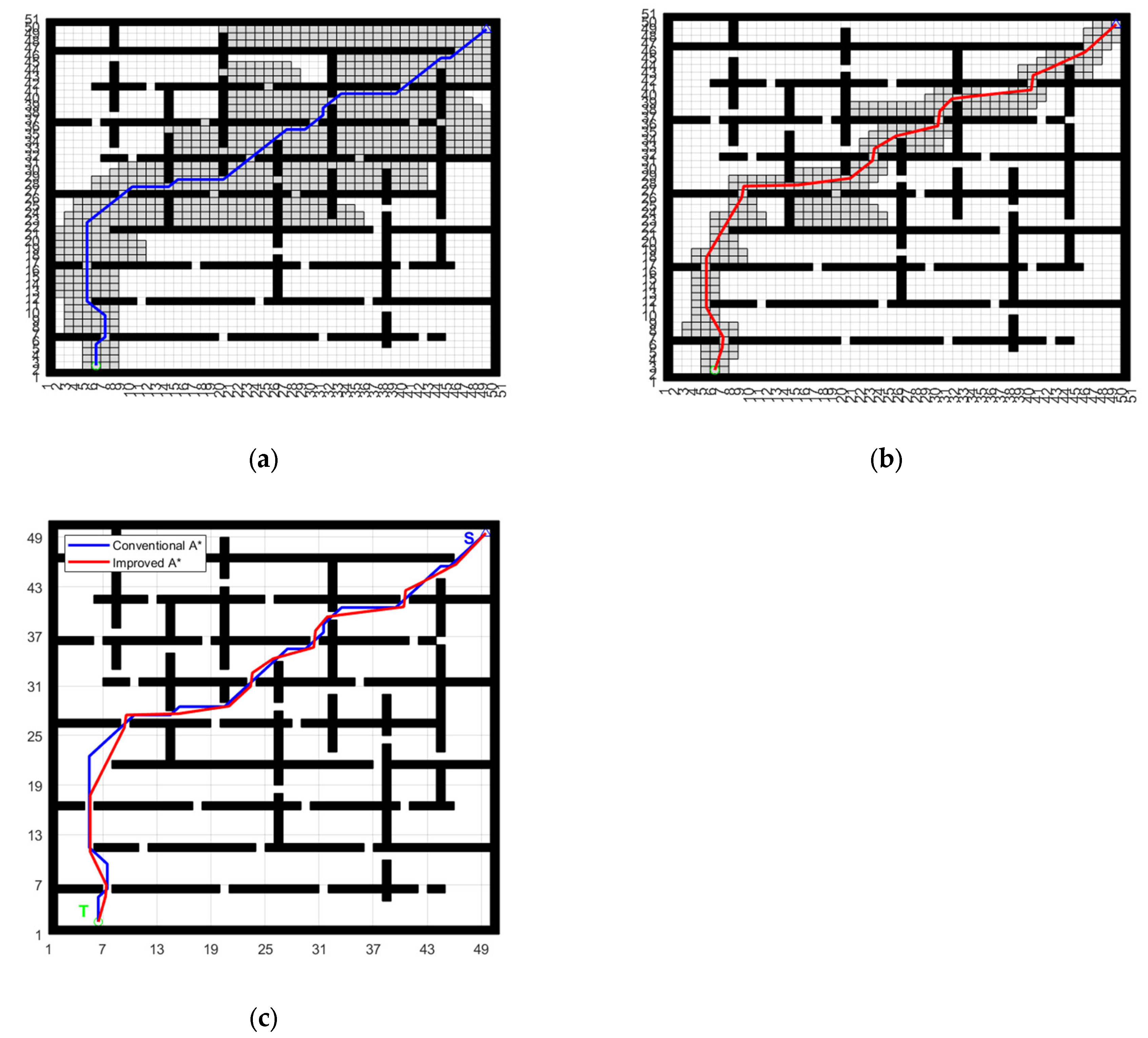
In the 50 × 50 grid map, the starting point was set at (49, 49), the target point at (1, 6), and the obstacle coverage was 27%. The path planning results for both the conventional A* and the improved A* are presented in Figure 9 and

Table 5. Comparison of path parameters on the 50 × 50 map.

Map	Algorithm	Planning Time/s	Turning Angle/°	Number of Turns	Path Length/m	Number of Nodes
50 × 50	Conventional A*	0.066 ± 0.015	765	17	77.01	791
	Improved A*	0.042 ± 0.015	630.21	19	76.59	303

.

As shown in Table 5, on the 50 × 50 grid map, the improved A* algorithm reduces the planning time by 35.93%, the turning angle by 17.62%, the path length by 0.54%, and the number of expanded nodes by 61.69%. Although the number of turns increases slightly, the decrease in the overall turning angle indicates that the path undergoes smoother global directional variation. This suggests that the proposed strategy may introduce more local directional adjustments while reducing large-angle directional changes. As a result, the path quality is improved without causing a significant deterioration in path executability.

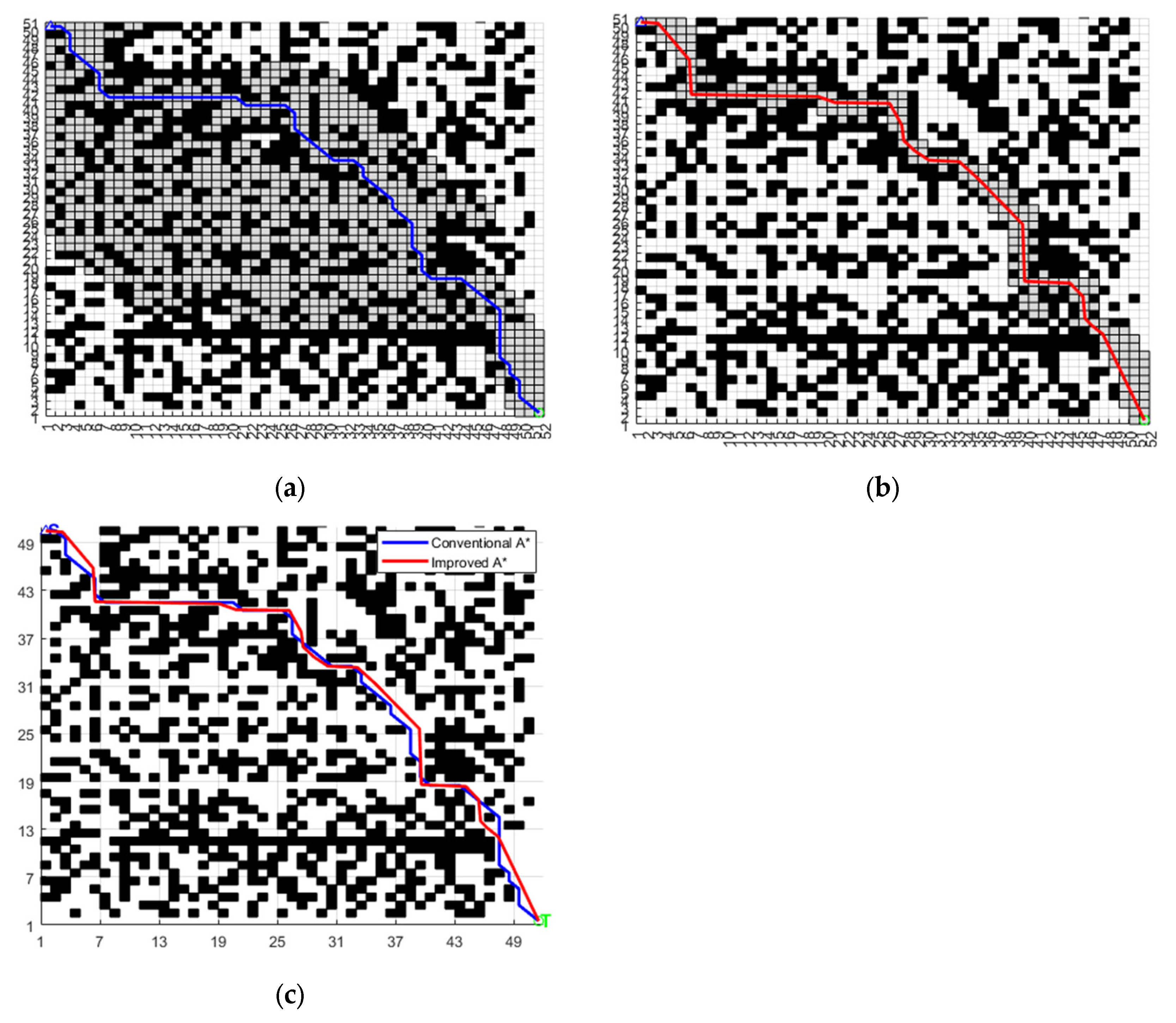
To assess the robustness of the proposed algorithm under more challenging obstacle configurations, a 50 × 50 extreme map was constructed. The map contains denser obstacles, narrow passages, block-shaped obstacle regions, and detour-required structures. In the 50 × 50 extreme map, the start point was set to (1, 50), the target point was set to (50, 1), and the obstacle coverage rate was 37.56%. The path planning results of the conventional A* and improved A* are shown in Figure 10 and

Table 6. Comparison of path parameters on the 50 × 50 extreme map.

Map	Algorithm	Planning Time/s	Turning Angle/°	Number of Turns	Path Length/m	Number of Nodes
50 × 50 extreme	Conventional A*	0.047 ± 0.012	1305	29	84.18	886
	Improved A*	0.014 ± 0.014	694.72	19	82.91	204

.

As shown in Table 6, in the 50 × 50 extreme map with dense obstacles and detour-required regions, both the conventional A* and improved A* successfully generated feasible paths. Compared with the conventional A*, the improved A* reduced the average expanded nodes from 886 to 204, corresponding to a reduction of 76.98%. Meanwhile, the average turning angle, number of turns, and path length decreased by 46.76%, 34.48%, and 1.51%, respectively. This demonstrates that the proposed direction-based search strategy, together with the adaptive evaluation and smoothing mechanisms, can maintain path feasibility while reducing redundant expansion and improving path quality in challenging obstacle configurations.

To further evaluate the statistical reliability of the planning-time comparison, a paired t-test was conducted on the repeated-run planning-time results. The significance level was set to 0.05. Since the path length, turning angle, number of turns, and expanded nodes remained unchanged across repeated runs in the same map, the t-test was mainly applied to the planning-time results.

As shown in

Table 7. Statistical significance analysis of planning time.

Map	Compared Methods	p-Value	Result
10 × 10	Improved A* vs. Conventional A*	0.0228	Significant difference
30 × 30		<0.001	Significant difference
50 × 50		<0.001	Significant difference
50 × 50 extreme		<0.001	Significant difference

, the paired t-test results show that the planning-time differences between the conventional A* and the improved A* are statistically significant at the 0.05 level in all tested maps. However, statistical significance only indicates that the difference is reliable; it does not necessarily mean that the improved algorithm is faster in every scenario. For example, in the 10 × 10 map, the improved A* algorithm has a longer planning time because the additional cost of adaptive evaluation and smoothing is more noticeable in simple environments.

The existing experiments on maps with different scales and obstacle complexities provide a preliminary observation of the influence of obstacle distribution on planning performance. In the 10 × 10 simple map, the improved A* algorithm reduces the turning angle and expanded nodes, but the planning time increases because the additional cost of adaptive evaluation and smoothing becomes more visible when the baseline search burden is low. In the 30 × 30 and 50 × 50 maps, the reduction in expanded nodes becomes more significant, indicating that the proposed adaptive strategy is more beneficial in more complex environments. In the 50 × 50 extreme map with dense obstacles and detour-required regions, the improved A* algorithm still maintains feasible path generation and significantly reduces expanded nodes, although the performance advantage should still be interpreted together with the map structure and obstacle distribution.

The turning-point smoothing strategy introduces an additional post-processing cost compared with the conventional A* algorithm. In relatively simple environments, where the search burden of conventional A* is already low, this additional overhead may become more visible in the total planning time. By contrast, in more complex environments, the reduction in redundant node expansion and the improvement in path quality become more significant, so the relative influence of the smoothing cost becomes less dominant.

Overall, the improved A* algorithm shows a scenario-dependent trade-off between search efficiency and path quality. In relatively simple environments, the additional cost introduced by adaptive evaluation and turning-point smoothing may lead to longer planning time and slightly longer path length, even though the path becomes smoother and the number of redundant nodes is reduced. By contrast, in more complex environments, the reduction in ineffective node expansion becomes more significant, and the advantages of the proposed strategy become more evident. Therefore, the proposed improvements are more suitable for complex maps, where the balance among search efficiency, path quality, and path smoothness is more favorable.

4.2. Simulation Experiments of the Fusion Algorithm with Static Obstacles

To evaluate the performance benefits of the proposed hybrid algorithm, a series of comparative simulation tests was carried out. Using the same experimental map, three approaches were examined: the hybrid method combining A* with the standard DWA, the M-A*-DWA method reported by Zhu et al., and the improved A*-GA-DWA hybrid approach developed in this study. In the simulated environment, the blue triangle denotes the starting position, the green circle denotes the goal position, the black grid cells correspond to known obstacles, the gray grid cells correspond to unknown static obstacles, and the yellow grid cells indicate dynamic obstacles.

To guarantee an equitable comparison, all compared fusion algorithms were implemented under the same simulation environment and shared the same basic DWA configuration. Specifically, the velocity constraints, acceleration constraints, velocity sampling resolution, angular velocity sampling resolution, prediction horizon, obstacle collision radius, and robot kinematic parameters were kept identical in the comparative experiments. Under this controlled setting, the performance differences are mainly attributed to the algorithmic design rather than to inconsistent parameter tuning. The main DWA and simulation parameter settings are summarized in

Table 8. Main DWA and simulation parameter settings used in the comparative experiments.

Parameter	Symbol	Setting
Maximum linear velocity	Vmax	3 m/s
Maximum angular velocity	ωmax	40°/s
Maximum linear acceleration	αmax	0.3 m/s2
Maximum angular acceleration	${\dot{\omega }}_{\mathrm{m}\mathrm{a}\mathrm{x}}$	100°/s2
Linear velocity resolution	Δv	0.03 m/s
Angular velocity resolution	Δω	1°/s
Prediction horizon	Tp	3 s
Obstacle collision radius	Robs	0.65 m

.

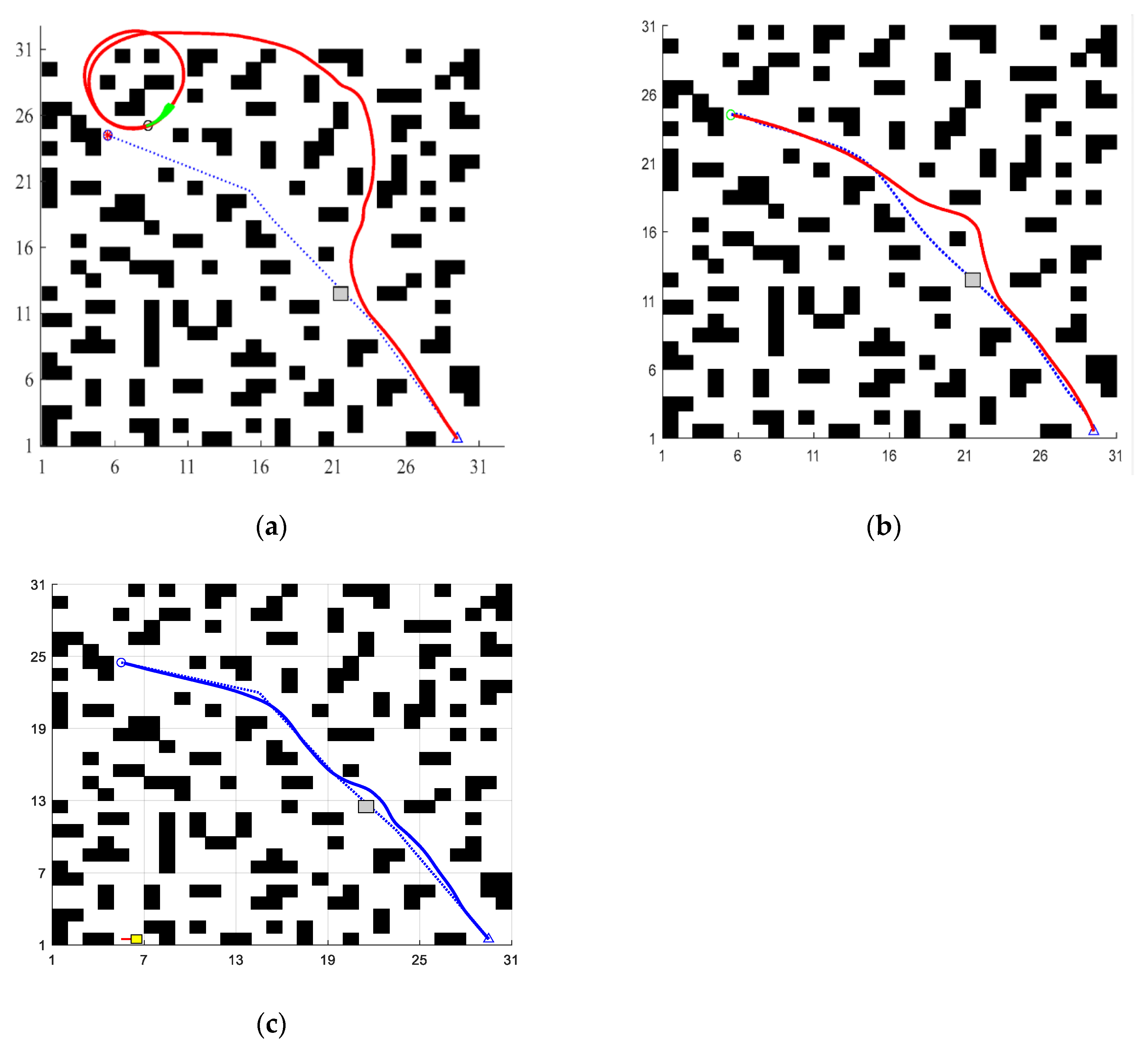
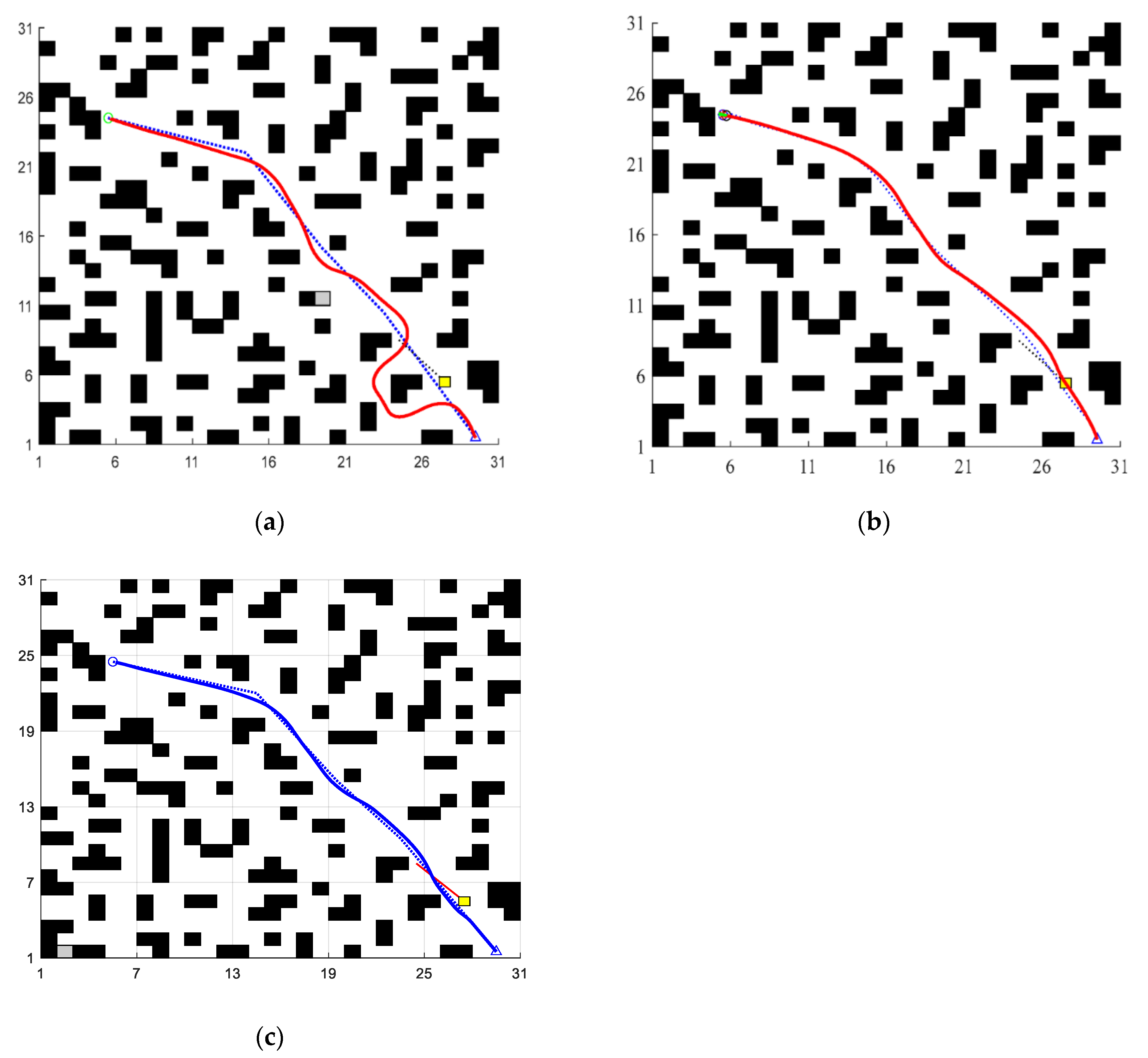
The test map is a 30 × 30 grid map, in which the start point is set to (1, 30) and the target point is set to (5, 24). An unknown static obstacle is placed at (21, 12). The path planning results are shown in Figure 11.

As shown in Figure 11, the conventional A*-DWA method shows clear limitations when the robot encounters newly introduced static obstacles. Although it can generate an avoidance trajectory, its local planning process may deviate significantly from the global route, resulting in a longer detour. Compared with A*-DWA, both M-A*-DWA and the proposed A*-GA-DWA method show better global–local coordination. In particular, the proposed A*-GA-DWA method can adjust the local trajectory more effectively after encountering the unknown static obstacle and then return to the global path more quickly. This indicates that the GA-optimized DWA evaluation function and key-node guidance strategy help improve obstacle-avoidance safety, trajectory continuity, and target reachability.

4.3. Simulation Experiments of the Fusion Algorithm with Dynamic Obstacles

The test map is a 30 × 30 grid map, where the start point is set to (1, 30) and the target point is set to (5, 24). The dynamic obstacle, represented by yellow cells, moves from (23, 8) to (27, 5). The path planning results are presented in Figure 12.

As shown in Figure 12, the conventional DWA algorithm is highly susceptible to the influence of dynamic obstacles, which leads to large fluctuations during robot motion. This not only reduces the stability of the robot in complex environments but also limits the overall performance of path planning and obstacle avoidance. When encountering dynamic obstacles, the M-A*-DWA algorithm also fails to avoid them effectively. In contrast, the A*-GA-DWA algorithm is capable of avoiding both known obstacles and unknown dynamic obstacles while maintaining stable robot motion and avoiding excessive adjustments. In addition, it can quickly return to the global path, and its trajectory conforms more closely to the global path, resulting in smoother motion. A comparison of the path parameters of the algorithms is given in

Table 9. Comparison of path parameters of different algorithms.

Algorithm	Path Length/m	Navigation Execution Time/s
A*-DWA	40.46	260.23
M-A*-DWA	34.88	178.48
A*-GA-DWA	34.76	140.58

.

To avoid ambiguity in the interpretation of the time-related indicators, two types of time are distinguished in this study. Planning computation time refers to the CPU runtime required by the planning algorithm and does not include robot motion execution, visualization, or rendering overhead. Navigation execution time refers to the total simulated time required for the robot to move from the start point to the target point under dynamic obstacle conditions, including the effects of local obstacle avoidance and replanning behavior. The time values reported in Table 9 correspond to navigation execution time rather than pure planning computation time.

As shown by the data in Table 9, the A*-GA-DWA algorithm yields the shortest path length and the lowest navigation execution time among the three algorithms, with values of only 34.76 m and 140.58 s, respectively. Compared with the conventional A*-DWA algorithm, the proposed fusion algorithm reduces the path length from 40.46 m to 34.76 m, corresponding to a decrease of approximately 14.07%, and shortens the navigation execution time from 260.23 s to 140.58 s, corresponding to a reduction of approximately 45.98%. Compared with the M-A*-DWA algorithm, the path length is reduced by approximately 0.32%, while the navigation execution time is reduced by approximately 21.23%. These results indicate that the proposed A*-GA-DWA algorithm can reduce path redundancy and improve task-completion efficiency in the dynamic-obstacle scenario. This improvement is mainly attributed to the coordinated effect of improved global path generation, GA-based DWA weight optimization, and key-node-guided local replanning.

These improvements should be understood as the result of a coordinated trade-off rather than a simple reduction in all performance indicators. On the one hand, the improved global path and key-node-guided sub-goals reduce unnecessary detours after obstacle avoidance. On the other hand, the GA-optimized DWA evaluation function improves the balance among heading, safety, and motion efficiency. Therefore, the observed reduction in path length and time is associated with stronger global–local coordination and fewer ineffective local adjustments in dynamic environments.

4.4. Additional Experiment

In order to evaluate the real-world performance of the proposed A*-GA-DWA, an additional experiment was conducted on a ROS-based mobile robot platform. Different from the MATLAB simulation, the ROS experiment was performed in a real indoor environment, where the robot needed to complete map-based navigation while perceiving surrounding obstacles through onboard sensors. The purpose of this experiment was to evaluate whether the proposed framework could be deployed in a robotic navigation system and whether the robot could follow the planned path while maintaining obstacle-avoidance capability.

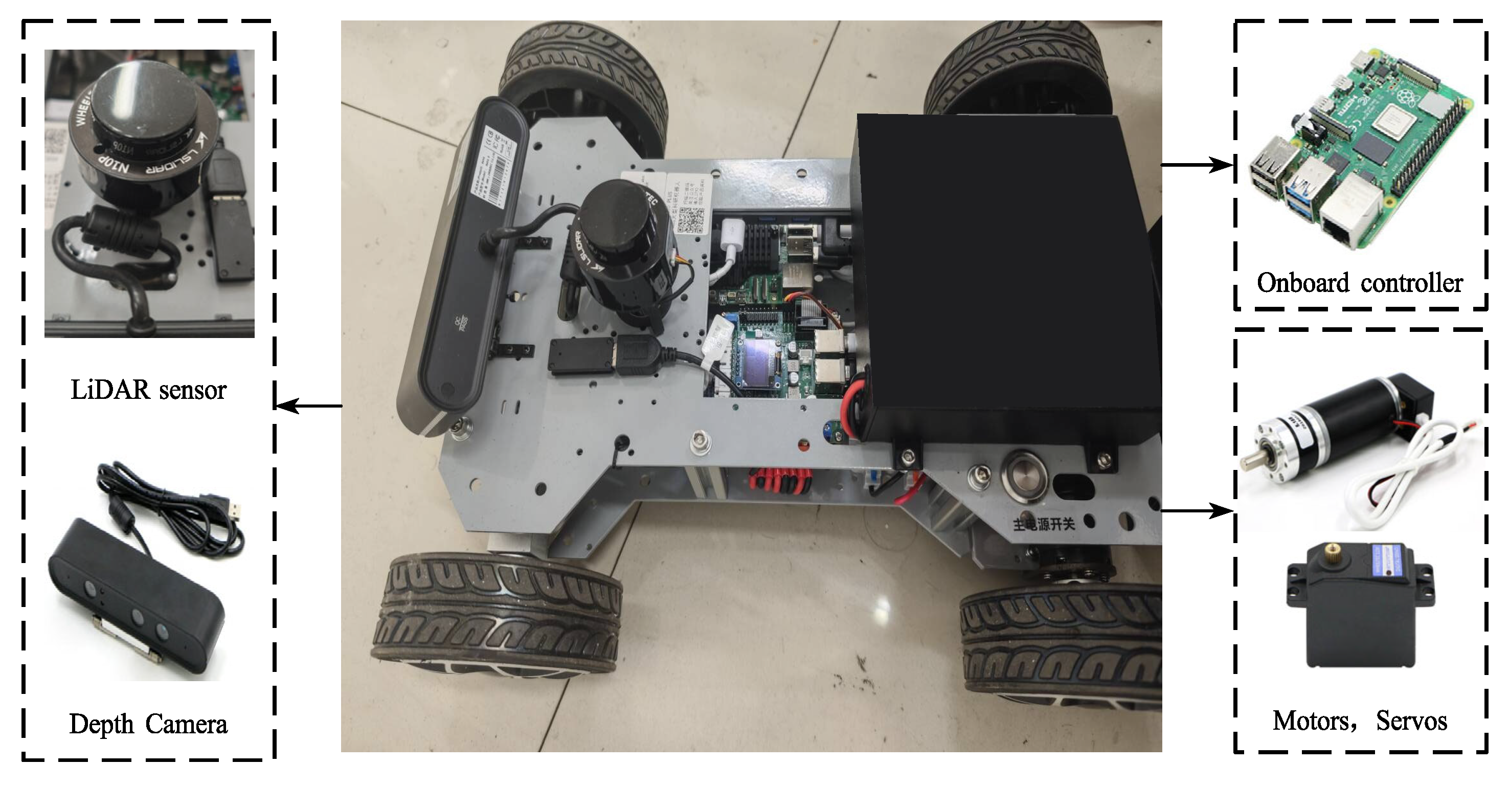
The experimental platform is shown in Figure 13. The robot platform mainly consists of a mobile chassis, an onboard controller, a LiDAR sensor, and a depth camera. The LiDAR was used to obtain environmental scan data, while the depth camera provided additional perception information for obstacle detection. The onboard controller was responsible for running the ROS navigation program, processing sensor data, generating the global path, and outputting velocity commands to the robot chassis. The main software environment was based on ROS, and RViz was used to visualize the map, robot pose, global path, local trajectory, and obstacle information.

During the experiment, the indoor environment was first mapped using the SLAM module. The LiDAR scan data and odometry information were fused to construct a two-dimensional occupancy grid map. After the map was built, the start point and target point were set in RViz. The preparatory work for the experiment is shown in Figure 14.

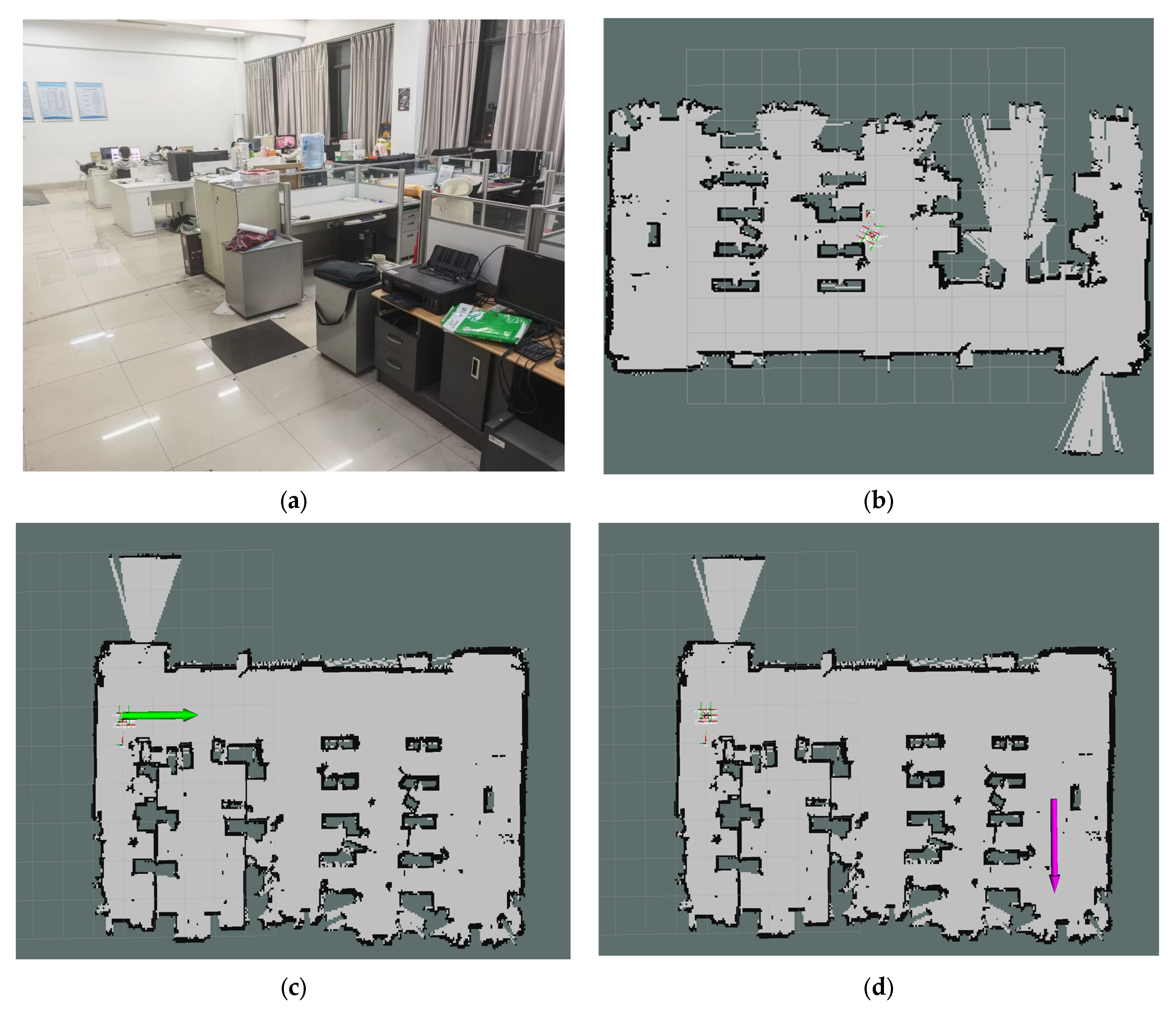
The overall ROS-based experimental procedure is as follows. First, the robot obtains the current pose through the localization module and receives the target point from RViz. Second, the improved A* algorithm plans a global path according to the occupancy grid map. Third, the key nodes are derived from the global path and sequentially provided to the DWA local planner as temporary sub-goals. Fourth, DWA samples candidate velocity commands within the dynamic window and selects the optimal velocity command according to the GA-optimized evaluation function. Finally, the selected velocity command is sent to the robot’s chassis, and the robot moves toward the target point while avoiding obstacles.

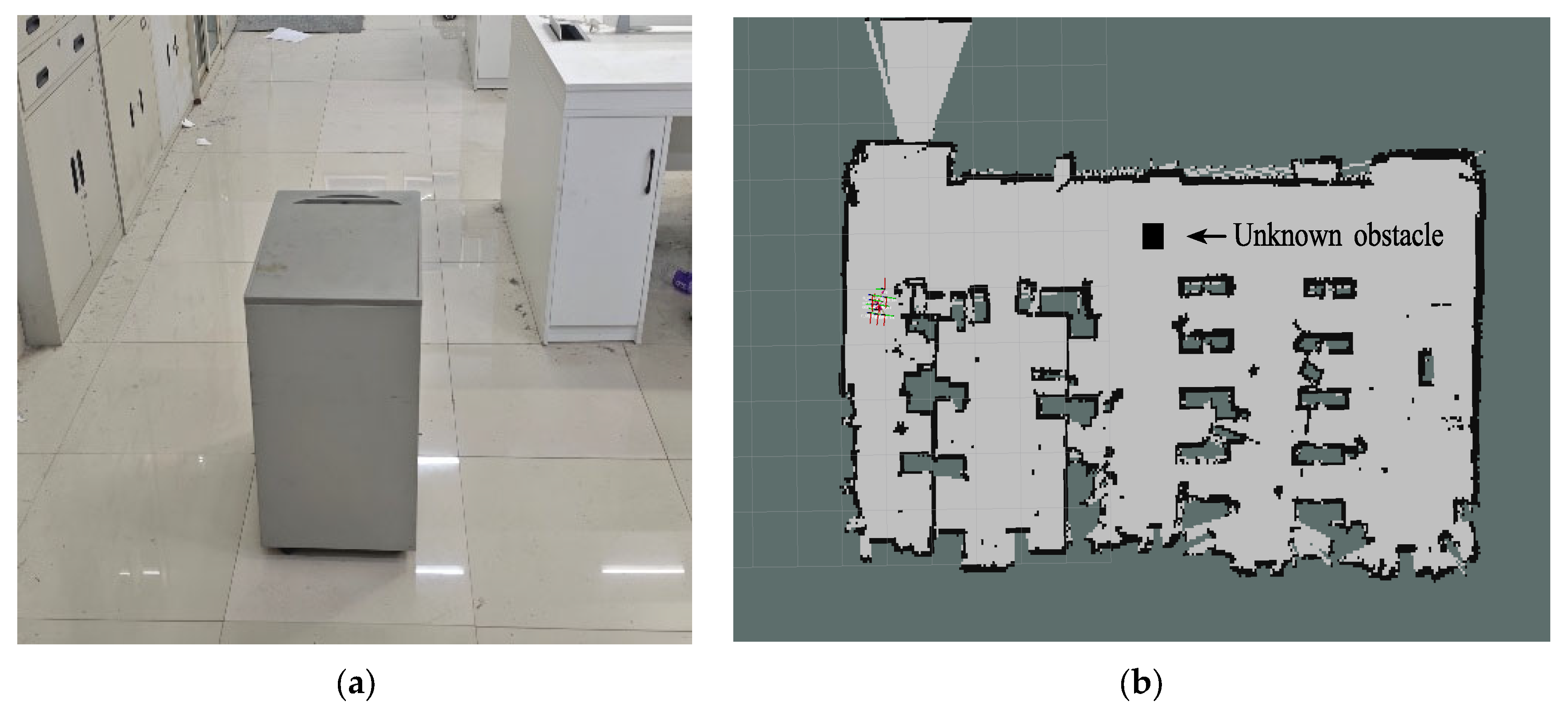
To further evaluate the local obstacle-avoidance capability of the proposed fusion framework, an unknown obstacle was placed on the planned path during the navigation process. Since this obstacle was not considered in the initial global path generation stage, the robot needed to rely on the local planner to respond to the newly detected obstacle. The location of the unknown obstacle is shown in Figure 15.

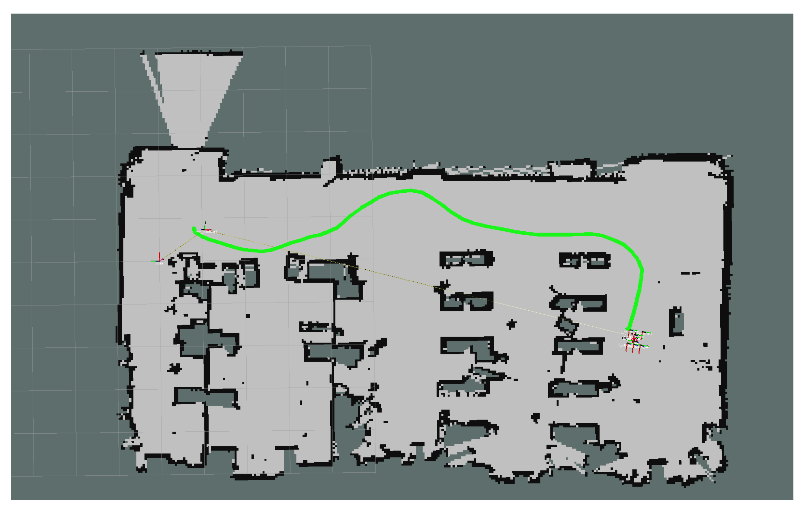
The ROS-based experimental result is shown in Figure 16. The robot successfully followed the global path generated by the improved A* algorithm under normal conditions. When an unknown obstacle appeared on the path, the robot adjusted its local trajectory in real time and avoided the obstacle without collision. After bypassing the obstacle, the robot returned to the guidance of the global path and continued toward the target point. This result indicates that the proposed A*-GA-DWA framework can maintain the consistency between global path planning and local obstacle avoidance, and it also demonstrates the effectiveness of the key-node-guided local planning strategy in a real ROS environment.

The additional experiment shows that the proposed A*-GA-DWA framework can complete map-based autonomous navigation and achieve local avoidance of unknown obstacles in a real environment. The robot successfully detected the unknown obstacle placed on the planned path, adjusted its local trajectory, avoided the obstacle without collision, and finally reached the target point. However, the current experiment was conducted in a relatively limited indoor scene. Future work will further evaluate the proposed method in larger and more complex environments, including multiple unknown obstacles, moving obstacles, and industrial scenarios with higher dynamic uncertainty.

5. Conclusions

To overcome the limitations of the conventional A* algorithm, such as excessive node expansion, numerous turning points, and low search efficiency in complex environments, along with the DWA algorithm’s tendency to converge to local optima, this paper proposes a mobile robot path planning algorithm that integrates the improved A* and DWA methods, referred to as A*-GA-DWA.

First, for the A* algorithm, a six-neighbor search-direction improvement strategy is proposed. In addition, an adaptive evaluation function based on environmental assessment is designed to improve search efficiency, and a turning-point smoothing strategy is introduced to optimize the path length and reduce the number of turns. Second, for the DWA algorithm, a GA-based evaluation function is developed to adaptively optimize DWA evaluation weights, significantly enhancing obstacle-avoidance performance in dynamic environments. Third, within the fusion framework, important nodes obtained from the global path produced by the A algorithm assist the DWA algorithm in local path planning and avoiding dynamic obstacles, thereby preventing it from converging to local optima.

Simulation results demonstrate that, on the designed 30 × 30 grid map, compared with the conventional A*-DWA algorithm, the proposed A*-GA-DWA algorithm reduces the average path length by 14.07% and shortens the average navigation execution time by 45.98%, while also generating a smoother path. This indicates that the improved search neighborhood is effective in reducing the number of search nodes and that the adaptive heuristic function contributes to accelerating the search process. Compared with the M-A*-DWA algorithm, the proposed algorithm reduces the path length by approximately 0.32% and shortens the navigation execution time by approximately 21.23%. Moreover, it can successfully avoid newly introduced static obstacles and dynamic obstacles, further confirming the effectiveness and applicability of the proposed method.

An additional ROS-based robot experiment was also conducted to verify the deployability of the proposed framework. In the experiment, an unknown obstacle was placed on the planned path. The robot successfully adjusted its local trajectory, avoided the unknown obstacle, and reached the target point. This result further verifies that the proposed A*-GA-DWA framework can be deployed in a ROS-based robotic navigation system and can support local obstacle avoidance in a real environment. Since the GA optimization is performed offline, the online navigation process does not require repeated evolutionary optimization, which reduces the online computational burden.

Nevertheless, this study still has certain limitations. The idealized robot kinematic model may deviate from actual complex operating conditions. In the presence of extremely complex road conditions and highly dynamic navigation scenarios, the accuracy and applicability of the model still need to be further improved. The present study mainly evaluates the overall performance of the proposed A*-GA-DWA framework. Although the functional role of each module has been clarified through mechanism analysis and experimental discussion, a complete quantitative ablation study of all modules under diverse static and dynamic environments has not yet been fully conducted. In future work, systematic ablation experiments will be designed by gradually enabling different modules to quantitatively evaluate their individual contributions to path length, expanded nodes, planning time, turning angle, and navigation execution time.

References

1. Jin, S.; Ke, K.; Gao, B.; Fu, L.; Huang, X. A Comprehensive Review of Key Technologies for Robot Motion Planning in Contact Tasks in Industrial Automation Scenarios. Chin. J. Mech. Eng. 2025, 38, 198. [Google Scholar] [CrossRef]
2. Bai, X.; Li, B.; Ullah, I.; Wu, Z.; Basheer, S.; Bashir, A.K. Energy-efficient routing for IoT-enabled multi-truck multi-drone pickup and delivery systems. Appl. Energy 2025, 400, 126546. [Google Scholar] [CrossRef]
3. Tang, Y.; Zakaria, M.A.; Younas, M. Path planning trends for autonomous mobile robot navigation: A review. Sensors 2025, 25, 1206. [Google Scholar] [CrossRef] [PubMed]
4. Lin, Z.; Wu, K.; Shen, R.; Yu, X.; Huang, S. An efficient and accurate A-star algorithm for autonomous vehicle path planning. IEEE Trans. Veh. Technol. 2024, 73, 9003–9008. [Google Scholar] [CrossRef]
5. Candra, A.; Budiman, M.A.; Hartanto, K. Dijkstra’s and A-star in finding the shortest path: A tutorial. In Proceedings of the 2020 International Conference on Data Science, Artificial Intelligence, and Business Analytics (DATABIA), Medan, Indonesia, 16–17 July 2020; pp. 28–32. [Google Scholar] [CrossRef]
6. Fu, B.; Chen, L.; Zhou, Y.; Zheng, D.; Wei, Z.; Dai, J.; Pan, H. An improved A* algorithm for the industrial robot path planning with high success rate and short length. Robot. Auton. Syst. 2018, 106, 26–37. [Google Scholar] [CrossRef]
7. Tang, G.; Tang, C.; Claramunt, C.; Hu, X.; Zhou, P. Geometric A-star algorithm: An improved A-star algorithm for AGV path planning in a port environment. IEEE Access 2021, 9, 59196–59210. [Google Scholar] [CrossRef]
8. Wu, D.; Du, K. A hybrid optimization algorithm of ACO and RRT for solving mobile robot path planning. Meas. Sci. Technol. 2025, 36, 076215. [Google Scholar] [CrossRef]
9. Gammell, J.D.; Srinivasa, S.S.; Barfoot, T.D. Informed RRT*: Optimal sampling-based path planning focused via direct sampling of an admissible ellipsoidal heuristic. In Proceedings of the 2014 IEEE/RSJ International Conference on Intelligent Robots and Systems (IROS), Chicago, IL, USA, 14–18 September 2014; pp. 2997–3004. [Google Scholar] [CrossRef]
10. Luo, Q.; Wang, H.; Zheng, Y.; He, J. Research on path planning of mobile robot based on improved ant colony algorithm. Neural Comput. Appl. 2020, 32, 1555–1566. [Google Scholar] [CrossRef]
11. Zhang, Z.; Yang, H.; Bai, X.; Zhang, S.; Xu, C. The path planning of mobile robots based on an improved genetic algorithm. Appl. Sci. 2025, 15, 3700. [Google Scholar] [CrossRef]
12. Yang, Y.; Luo, X.; Li, W.; Liu, C.; Ye, Q.; Liang, P. AAPF*: A safer autonomous vehicle path planning algorithm based on the improved A* algorithm and APF algorithm. Clust. Comput. 2024, 27, 11393–11406. [Google Scholar] [CrossRef]
13. Weerakoon, T.; Ishii, K.; Nassiraei, A.A.F. An artificial potential field based mobile robot navigation method to prevent from deadlock. J. Artif. Intell. Soft Comput. Res. 2015, 5, 189–203. [Google Scholar] [CrossRef]
14. Hu, Y.; Chen, X.; Tang, P.; Zhang, H.; Jin, J.; Mao, S. A path planning framework for robots based on improved parallel sampling RRT and offset guidance DWA. IEEE Sens. J. 2025, 25, 35597–35608. [Google Scholar] [CrossRef]
15. Tao, X.; Lang, N.; Li, H.; Xu, D. Path planning in uncertain environment with moving obstacles using warm start cross entropy. IEEE/ASME Trans. Mechatron. 2022, 27, 800–810. [Google Scholar] [CrossRef]
16. Kala, R.; Shukla, A.; Tiwari, R. Fusion of probabilistic A* algorithm and fuzzy inference system for robotic path planning. Artif. Intell. Rev. 2010, 33, 307–327. [Google Scholar] [CrossRef]
17. Wang, X.; Lu, J.; Ke, F.; Wang, X.; Wang, W. Research on AGV task path planning based on improved A* algorithm. Virtual Real. Intell. Hardw. 2023, 5, 249–265. [Google Scholar] [CrossRef]
18. Xu, X.; Zeng, J.; Zhao, Y.; Lü, X. Research on global path planning algorithm for mobile robots based on improved A*. Expert Syst. Appl. 2024, 243, 122922. [Google Scholar] [CrossRef]
19. Zammit, C.; Van Kampen, E.J. Comparison between A* and RRT algorithms for 3D UAV path planning. Unmanned Syst. 2022, 10, 129–146. [Google Scholar] [CrossRef]
20. Berti, H.; Sappa, A.D.; Agamennoni, O.E. Improved dynamic window approach by using Lyapunov stability criteria. Lat. Am. Appl. Res. 2008, 38, 289–298. [Google Scholar]
21. Kang, Y.; de Lima, D.A.; Victorino, A.C. Dynamic obstacles avoidance based on image-based dynamic window approach for human-vehicle interaction. In Proceedings of the 2015 IEEE Intelligent Vehicles Symposium (IV), Seoul, Republic of Korea, 28 June–1 July 2015; pp. 77–82. [Google Scholar] [CrossRef]
22. Henkel, C.; Bubeck, A.; Xu, W. Energy efficient dynamic window approach for local path planning in mobile service robotics. IFAC-PapersOnLine 2016, 49, 32–37. [Google Scholar] [CrossRef]
23. Lai, X.; Wu, D.; Wu, D.; Li, J.H.; Yu, H. Enhanced DWA algorithm for local path planning of mobile robot. Ind. Robot 2023, 50, 186–194. [Google Scholar] [CrossRef]
24. Luo, Y.; Lin, S.; Wang, Y.; Liang, K. Path planning for mobile robots in complex environments based on enhanced sparrow search algorithm and dynamic window approach. Robotica 2025, 43, 1929–1952. [Google Scholar] [CrossRef]
25. Zhu, W.; Chen, Z. Research on path planning for mobile charging robots based on improved A* and DWA algorithms. Electronics 2025, 14, 2318. [Google Scholar] [CrossRef]
Figure 1. Schematic diagram of search directions.
Electronics 15 02308 g001
Figure 2. Kinematic modeling of the mobile robot.
Electronics 15 02308 g002
Figure 3. Determination of turning directions at turning points.
Electronics 15 02308 g003
Figure 4. Schematic illustration of turning-point folding. (a) First folding; (b) second folding; (c) third folding; (d) folding completed.
Electronics 15 02308 g004aElectronics 15 02308 g004b
Figure 5. Schematic illustration of the improved path after turning-point smoothing.
Electronics 15 02308 g005
Figure 6. Flowchart of the fusion algorithm.
Electronics 15 02308 g006
Figure 7. Comparison of path planning results on the 10 × 10 grid map. (a) Search path of the conventional A* algorithm; (b) search path of the improved A* algorithm; (c) path comparison.
Electronics 15 02308 g007
Figure 8. Comparison of path planning results on the 30 × 30 grid map. (a) Search path of the conventional A* algorithm; (b) search path of the improved A* algorithm; (c) path comparison.
Electronics 15 02308 g008
Figure 9. Comparison of path planning results on the 50 × 50 grid map. (a) Search path of the conventional A* algorithm; (b) search path of the improved A* algorithm; (c) path comparison.
Electronics 15 02308 g009
Figure 10. Comparison of path planning results on the 50 × 50 extreme map. (a) Search path of the conventional A* algorithm; (b) search path of the improved A* algorithm; (c) path comparison.
Electronics 15 02308 g010
Figure 11. Obstacle avoidance performance in the presence of static obstacles. (a) A*-DWA path; (b) M-A*-DWA path; (c) A*-GA-DWA path.
Electronics 15 02308 g011
Figure 12. Obstacle avoidance performance in the presence of dynamic obstacles. (a) A*-DWA path; (b) M-A*-DWA path; (c) A*-GA-DWA path.
Electronics 15 02308 g012
Figure 13. Mobile robot platform.
Electronics 15 02308 g013
Figure 14. Preparatory work for the experiment. (a) Indoor environment; (b) scanned map; (c) setting the start point; (d) setting the target point.
Electronics 15 02308 g014
Figure 15. Location of the unknown obstacle. (a) Actual location; (b) location on the map.
Electronics 15 02308 g015
Figure 16. Experimental results on mobile robot navigation.
Electronics 15 02308 g016