Enhanced Composite Multi-Scale Slope Entropy and Its Application to Fault Diagnosis of Rolling Bearing

Abstract

The health status of rolling bearings is critical to the normal operation of rotating machinery. To effectively extract vibration signal features and accurately identify different fault types, a novel method based on enhanced composite multi-scale slope entropy (ECMSE) and a honey badger algorithm-optimized kernel extreme learning machine (HBA–KELM) is proposed. Specifically, ECMSE integrates high-order differences into the composite multi-scale framework to capture high-frequency information while preserving low-frequency characteristics, thereby enhancing the discriminability of time-series representations. Meanwhile, an average coarse-graining strategy is incorporated to achieve a more comprehensive characterization of the signals. The extracted features are then input into the HBA–KELM classifier for fault identification. Experiments conducted on two public and private rolling bearing datasets demonstrate that our method achieves superior performance in distinguishing different fault types and damage levels compared with several existing approaches.

1. Introduction

Rolling bearings are essential components in most rotating machinery, and their operating conditions have a considerable impact on the normal operation of mechanical systems. Rolling bearing failures often lead to serious safety issues and economic losses. Therefore, accurate and timely fault detection of rolling bearings has become increasingly important [1,2,3,4,5,6].

In practical scenarios, fault signals are typically non-stationary and nonlinear, and are often contaminated with significant noise, making early fault information difficult to detect. Traditional approaches usually analyze signals in the time or frequency domain, but they are less effective in identifying fault characteristics. Therefore, time–frequency analysis methods have been widely adopted for feature extraction, such as wavelet transform (WT) [7], complete ensemble empirical mode decomposition with adaptive noise (CEEMDAN) [8], variational mode decomposition (VMD) [9], and Fourier decomposition method (FDM) [10]. However, these methods still have limitations in practical applications. For instance, the performance of WT is highly dependent on the selection of basis functions. CEEMDAN may introduce noise and spurious components in the early intrinsic mode functions. VMD requires manual determination of decomposition layers and penalty factors, and is not suitable for signals with complex and dense modes. In addition, FDM may produce inconsistent results under different search strategies, and its iterative process is time-consuming. Consequently, effective application of these methods often requires substantial prior knowledge and experience, and their inherent limitations are difficult to overcome.

In addition to purely data-driven signal processing, physics-guided modeling has recently received increasing attention in bearing health monitoring. For example, physics-guided degradation trajectory modeling and trustworthy multi-step prediction attempt to constrain remaining useful life prediction using degradation consistency and reliability-aware mechanisms [11,12], while fault-evolution-knowledge-driven learning introduces prior fault evolution information to improve adaptation across changing working conditions [13]. These studies indicate that bearing diagnosis can benefit from combining data-driven representations with mechanical prior knowledge. Nevertheless, many physics-guided methods require explicit degradation trajectories, cross-condition labels, or prior knowledge of fault evolution, which may be unavailable in short-sample fault classification scenarios. Therefore, this study focuses on constructing a compact and interpretable entropy-based representation that captures both low-frequency state variation and high-frequency fault-related details from vibration signals.

Entropy is an effective tool for measuring the complexity of time series and has been widely used in signal feature extraction across various domains [14,15]. Methods such as approximate entropy (AE) [16], fuzzy entropy (FE) [17], and permutation entropy (PE) [18] have been successfully applied in rolling bearing fault diagnosis. Among them, PE is widely used due to its computational simplicity and efficiency. However, PE only evaluates the complexity of a single-scale sequence. To address this limitation, multi-scale permutation entropy (MPE) [19] was proposed to extract information across multiple scales and improve robustness. Nevertheless, MPE still has several drawbacks: (1) the coarse-grained sequence becomes shorter as the scale factor increases, leading to the loss of useful information; (2) PE ranks subsequences based on relative amplitudes while ignoring their actual values, which may map significantly different sequences into the same pattern. To overcome these issues, Zheng et al. [20] proposed composite multi-scale weighted permutation entropy (CMWPE), which combines composite multi-scale processing with weighted permutation entropy (WPE) [21] to better distinguish sequence differences using variance. In addition to WPE, its variants such as fine-grained permutation entropy (FGPE) [22] and amplitude-aware permutation entropy (AAPE) [23] have also shown similar improvements.

Recently, slope entropy (SE) [24] was proposed to encode the slopes between adjacent amplitudes into symbolic patterns and characterize the dynamic properties of time series. SE is more sensitive to amplitude fluctuations and requires fewer samples to achieve statistical significance. It has also been demonstrated that SE outperforms WPE, FGPE, and AAPE in various applications. Based on this, composite multi-scale slope entropy (CMSE) is obtained by combining SE with composite multi-scale analysis. However, the traditional coarse-graining method generates short sequences at different scales and mainly captures low-frequency information [25]. Moreover, sequences with identical average values may still differ significantly in amplitude distribution and arrangement.

To address these issues and capture high-frequency information, multi-order differences are introduced in this study to replace the average coarse-graining process, resulting in difference-based composite multi-scale slope entropy (DBCMSE). Furthermore, to achieve a more comprehensive representation of time series, an enhanced composite multi-scale slope entropy (ECMSE) method is proposed by combining CMSE and DBCMSE. ECMSE considers both amplitude information and multi-frequency characteristics, while being less sensitive to data length, thereby providing a more effective representation of rolling bearing health conditions. After feature extraction using ECMSE, the obtained feature vectors are input into a classifier for intelligent fault diagnosis. Kernel extreme learning machine (KELM) [26] extends extreme learning machine (ELM) by incorporating kernel functions and generally achieves better generalization performance. However, its performance is sensitive to the selection of regularization coefficients and kernel parameters. To address this issue, the honey badger algorithm (HBA) [27] is employed to optimize the parameters of KELM adaptively. Based on the above methods, a novel intelligent fault diagnosis framework for rolling bearings is proposed. Finally, two rolling bearing datasets are used to validate the effectiveness and reliability of the proposed method in identifying faults with different types and damage levels.

The remainder of this paper is organized as follows. Section 2 introduces the theory and parameter selection of ECMSE. Section 3 presents the HBA–KELM method. Section 4 provides experimental validation, and Section 5 concludes the paper.

2. Slope-Entropy-Based Feature Extraction Methods

2.1. Slope Entropy

For a given one-dimensional time series $x={\left\{x_i\right\}}_{i=1}^L$ of length L, the phase space of x can be reconstructed, and the subspace sequences are defined as

$$X_m^t=\{x_t,x_{t+\tau },\dots ,x_{t+\tau (m-2)},x_{t+\tau (m-1)}\},$$

(1)

where $t=1,2,\dots ,L-\tau (m-1)$, m denotes the embedding dimension, and $\tau$ denotes the time delay.

Then, a vertical increment threshold $\gamma$ (high threshold) is defined to measure significant differences between elements, and a zero-difference threshold $\delta$ (low threshold) is introduced to characterize cases with approximately equal amplitudes. Next, $X_m^t$ is transformed into a symbolic subsequence based on adjacent differences and predefined thresholds. The procedure for defining slopes as symbols is illustrated in Figure 1.

In Figure 1, $\Delta x$ denotes the difference between two adjacent elements in the reconstructed vector. The symbols $+2$ and $-2$ represent positive and negative slopes whose absolute amplitudes exceed the high threshold $\gamma$, respectively; $+1$ and $-1$ represent moderate positive and negative slopes between the low threshold $\delta$ and the high threshold $\gamma$, respectively; and 0 represents an approximately unchanged amplitude interval satisfying $|\Delta x|\le \delta$.

The probability of each symbolic subsequence pattern is calculated as

$$p_i={\displaystyle \frac{h_i}{N_s}},$$

(2)

where $h_i$ denotes the number of occurrences of the i-th pattern, and $N_s$ represents the total number of symbolic subsequences. Let K denote the number of observed symbolic patterns.

Finally, based on Shannon entropy, slope entropy is defined as

$$SE=-{\displaystyle \sum _{i=1}^K}{p}_i{log}_2\left(p_i\right).$$

(3)

2.2. Composite Multi-Scale Slope Entropy

The composite coarse-graining technique generates multiple subsequence combinations, thereby reducing entropy fluctuations and improving robustness compared with the traditional multiscale method. By combining it with slope entropy, composite multi-scale slope entropy (CMSE) is obtained. For a given one-dimensional time series $x={\left\{x_i\right\}}_{i=1}^L$ of length L, the average coarse-grained sequences $y_k^{\left(s\right)}=\{y_{k,1}^{\left(s\right)},y_{k,2}^{\left(s\right)},\dots ,y_{k,q}^{\left(s\right)}\}$ are defined as

$$y_{k,j}^{\left(s\right)}={\displaystyle \frac{1}{s}}{\displaystyle \sum _{i=(j-1)s+k}^{js+k-1}}{x}_i,$$

(4)

where $1\le j\le q=\lfloor L/s\rfloor$, $1\le k\le s$, and $s=1,2,\dots ,s_{max}$. Here, $\lfloor ·\rfloor$ denotes the floor operator, $s_{max}$ is the maximum scale factor, and $y_k^{\left(s\right)}$ represents the k-th coarse-grained sequence at scale s.

Then, the SE values of each coarse-grained sequence are computed, and CMSE is defined as

$$CMSE(x,s,m,\tau ,\gamma ,\delta )={\displaystyle \frac{1}{s}}{\displaystyle \sum _{k=1}^s}SE(y_k^{\left(s\right)},m,\tau ,\gamma ,\delta ).$$

(5)

2.3. Difference-Based Composite Multi-Scale Slope Entropy

To capture high-frequency information and reveal details that CMSE may overlook, difference-based composite multi-scale slope entropy (DBCMSE) is proposed by replacing the average coarse-graining method with a multi-order difference scheme. For a given one-dimensional time series $x={\left\{x_i\right\}}_{i=1}^L$ of length L, the $(s-1)$-order difference is applied under scale factor $s>1$. The difference-based sequences $z_k^{\left(s\right)}=\{z_{k,1}^{\left(s\right)},z_{k,2}^{\left(s\right)},\dots ,z_{k,q}^{\left(s\right)}\}$ are defined as

$$z_{k,j}^{\left(s\right)}={\displaystyle \sum _{i=(j-1)s+k}^{js+k-1}}{(-1)}^{s-1-a}\left({\displaystyle \genfrac{}{}{0pt}{}{s-1}{a}}\right)x_i,$$

(6)

where $a=i-\left[\right(j-1)s+k]$, $1\le j\le q=\lfloor L/s\rfloor$, $1\le k\le s$, and $s=1,2,\dots ,s_{max}$. Here, $\left({\displaystyle \genfrac{}{}{0pt}{}{s-1}{a}}\right)$ denotes the binomial coefficient, and $z_k^{\left(s\right)}$ represents the k-th difference-based sequence at scale s.

Similar to CMSE, DBCMSE is defined as

$$DBCMSE(x,s,m,\tau ,\gamma ,\delta )={\displaystyle \frac{1}{s}}{\displaystyle \sum _{k=1}^s}SE(z_k^{\left(s\right)},m,\tau ,\gamma ,\delta ).$$

(7)

2.4. Enhanced Composite Multi-Scale Slope Entropy

To incorporate both low- and high-frequency information, CMSE and DBCMSE are averaged. The enhanced composite multi-scale slope entropy (ECMSE) is defined as

$$ECMSE(x,s,m,\tau ,\gamma ,\delta )={\displaystyle \frac{CMSE(x,s,m,\tau ,\gamma ,\delta )+DBCMSE(x,s,m,\tau ,\gamma ,\delta )}{2}}.$$

(8)

The equal-weight fusion is adopted because CMSE and DBCMSE are two parallel descriptions generated from the same original signal and share the same scale factor, embedding dimension, time delay, and slope thresholds. CMSE emphasizes the low-frequency trend retained by local averaging, whereas DBCMSE emphasizes high-frequency amplitude variation produced by the difference operator. Assigning equal weights avoids introducing an additional data-dependent hyperparameter during feature extraction and reduces the risk of overfitting when only a small number of training samples are available. Therefore, ECMSE can be interpreted as a two-branch multi-resolution entropy representation that balances low-frequency trend information and high-frequency fault details in an unsupervised manner.

The implementation procedure of ECMSE is illustrated in Figure 2. The traditional coarse-graining method is analogous to an arithmetic mean filter, which can suppress noise but may obscure fine-scale details and reduce frequency information [28]. In contrast, the multi-order difference method can be regarded as a weighting operation and exhibits high-pass filtering characteristics. For example, the weights are $\{-1,1\}$ at scale $s=2$, and $\{1,-2,1\}$ at scale $s=3$. As shown in Figure 3, the normalized spectra indicate that the multi-order difference operation behaves as a high-pass filter, with the cutoff frequency increasing as the scale factor increases.

From a numerical perspective, the two methods may produce different outputs. For instance, subsequences $\{1,3,5\}$ and $\{2,4,3\}$ yield the same average value but different outputs under the difference-based method. Similarly, sequences with identical elements but different permutations can be distinguished by the difference-based method, while the coarse-graining method produces identical results. However, the difference-based method cannot distinguish sequences with the same linear trend. Therefore, the two approaches are complementary, and their combination leads to improved performance.

As shown in Figure 2, ECMSE first reconstructs the original signal at multiple scales. In the CMSE branch, average coarse-graining is used to obtain low-frequency subsequences, and SE is then calculated for each composite subsequence. In the DBCMSE branch, the multi-order difference operation is used to obtain high-frequency-sensitive subsequences before SE calculation. Finally, the entropy values of the two branches are averaged at each scale to form the ECMSE feature vector.

2.5. Parameter Selection of ECMSE

The performance of ECMSE depends on the embedding dimension m, time delay $\tau$, maximum scale factor $s_{max}$, low threshold $\delta$, high threshold $\gamma$, and sample length L. In this study, $\tau =1$ and $s_{max}=8$ are set according to [29]. To determine appropriate thresholds, we set

$$\delta \in \{{10}^{-1},{10}^{-2},{10}^{-3},{10}^{-4},{10}^{-5},{10}^{-6}\},$$

(9)

and

$$\gamma \in \{30°,45°,60°\}.$$

(10)

The embedding dimension is selected from

$$m\in [2,7].$$

(11)

To determine the optimal parameters, the mean silhouette coefficient (MSC) is used to evaluate clustering performance. MSC ranges from $-1$ to 1, and higher values indicate better feature separability. It is defined as

$$MSC={\displaystyle \frac{1}{N}}{\displaystyle \sum _{i=1}^N}\left({\displaystyle \frac{b\left(i\right)-a\left(i\right)}{max\left\{a\right(i),b(i\left)\right\}}}\right),$$

(12)

where $a\left(i\right)$ represents intra-class cohesion and $b\left(i\right)$ denotes the minimum inter-class distance.

Finally, different sample lengths are evaluated to analyze robustness. Considering both stability and computational efficiency, $L=1024$ is selected. As illustrated in Figure 4, the overall trends of the entropy curves for different sample lengths are generally consistent. However, when $L=512$, the entropy values of both noise signals deviate from this trend, and the curve of the $1/f$ noise exhibits a more pronounced offset along with larger standard deviations.

3. Honey Badger Algorithm Optimized Kernel Extreme Learning Machine

3.1. Honey Badger Algorithm

HBA is a biological heuristic algorithm that simulates the activity of a honey badger colony searching for a beehive. In the search phase, if the smell of food is strong, their movement intensifies, and vice versa. Compared with traditional metaheuristic optimizers such as particle swarm optimization (PSO) and genetic algorithm (GA), HBA combines two search behaviors: a digging phase for local exploitation around the current best solution and a honeyguide-bird phase for global exploration. The density factor decreases adaptively with iterations, which helps the search process move gradually from exploration to exploitation. In addition, HBA has relatively few control parameters, making it convenient for optimizing the regularization coefficient and kernel width of KELM. The key HBA–KELM parameter settings used in this study are listed in

Table 1. Key parameter settings of HBA–KELM.

Parameter	Value
Population size	20
Maximum number of iterations	50
Density factor constant C	2
Ability coefficient $\beta$	6
Search range of KELM regularization coefficient A	$[2^{-8},2^8]$
Search range of RBF kernel width $\sigma$	$[2^{-8},2^8]$
Fitness function	Training classification error rate

.

The search procedure of HBA is as follows:

(1) Initializing the honey badger colony:

$$x_i=l{b}_i+r_1\times (u{b}_i-l{b}_i)$$

(13)

where $x_i$ represents the position of the i-th honey badger, $r_1$ is a random number in $[0,1]$, $u{b}_i$ and $l{b}_i$ represent the upper and lower search bounds, respectively.

(2) Defining intensity: Smell intensity $I_i$ is determined by source strength S and the distance $d_i$:

$$\begin{array}{c}{I}_i=r_2\times {\displaystyle \frac{S}{4\pi d_i^2}}\end{array}$$

(14)

$$\begin{array}{c}S={(x_i-x_{i+1})}^2\end{array}$$

(15)

$$\begin{array}{c}{d}_i=x_{\mathrm{prey}}-x_i\end{array}$$

(16)

where $r_2$ is a random number in $[0,1]$, and $x_{\mathrm{prey}}$ is the best prey location found so far.

(3) Updating density factor: The factor $\alpha$ ensures search stability:

$$\alpha =C\times exp\left({\displaystyle \frac{-t}{t_{max}}}\right)$$

(17)

where C is a constant (default $=2$) and $t_{max}$ is the maximum number of iterations.

(4) Digging and honeyguide bird phase: The behavior is determined by r, a random number in $[0,1]$. When $0\le r<0.5$, the position $x_{\mathrm{new}}$ is updated as:

$$x_{\mathrm{new}}=x_{\mathrm{prey}}+F\times \beta \times I\times x_{\mathrm{prey}}+F\times r_3\times \alpha \times d_i\times |cos\left(2\pi r_4\right)\times [1-cos\left(2\pi r_5\right)]|$$

(18)

The direction factor F is defined as:

$$F=\left\{\begin{array}{cc}1\hfill & \mathrm{if}{r}_6\le 0.5\hfill \\ -1\hfill & \mathrm{if}{r}_6>0.5\hfill \end{array}\right.$$

(19)

3.2. Kernel Extreme Learning Machine

According to Mercer’s theorem, the kernel function $\Omega$ is defined as:

$$\Omega =H{H}^T,\Omega (i,j)=h\left(x_i\right)h\left(x_j\right)=K(x_i,x_j)$$

(20)

The output of the network can be expressed as:

$$g\left(x\right)=\left[K(x,x_1),\dots ,K(x,x_N)\right]{\left({\displaystyle \frac{I}{A}}+\Omega \right)}^{-1}T$$

(21)

The radial basis function (RBF) is selected as the kernel:

$$K(x_i,x_j)=exp\left(-{\displaystyle \frac{\parallel x_i-x_j{\parallel }^2}{2{\sigma }^2}}\right)$$

(22)

3.3. HBA–KELM Algorithm (Continued)

(5) Honeyguide bird phase: When $r\ge 0.5$, the position is updated according to the following strategy:

$$x_{\mathrm{new}}=x_{\mathrm{prey}}+F\times r_7\times \alpha \times d_i$$

(23)

Based on the HBA and KELM, the initial parameters $(A,\sigma )$ of the KELM are optimized using the HBA. The classification error rate of the training set is selected as the fitness function for the HBA–KELM:

$$\mathrm{fitness}\left(x\right)={\displaystyle \frac{N_{\mathrm{err}}}{N_{\mathrm{train}}}}$$

(24)

where $N_{\mathrm{err}}$ is the number of incorrectly classified training samples and $N_{\mathrm{train}}$ is the total number of training samples. A smaller fitness value indicates better KELM parameters.

3.4. Implementation of the Proposed Method

To accurately identify rolling bearings under different health conditions, an intelligent fault diagnosis method based on ECMSE and HBA–KELM is proposed. To improve the recognition accuracy of KELM, the global optimization capability of HBA is utilized to achieve automatic parameter selection of KELM, thereby establishing a fault diagnosis model for rolling bearings.

The flowchart of the proposed method is shown in Figure 5, and the detailed procedure is as follows:

• Acceleration sensors are used to collect vibration signals of rolling bearings under different health conditions.
• For each fault type, M samples with length $L=1024$ are obtained. Then, N samples are randomly selected as the training set, and the remaining $M-N$ samples are used as the test set.
• After the training/test split is completed in each run, the MSC values of random feature samples from the training set only are calculated under different parameter combinations $(\delta ,\gamma ,m)$ to determine the optimal ECMSE parameters. First, the time delay is set to $\tau =1$, and the maximum scale factor is set to $s_{max}=8$. The low threshold $\delta$ is only used to categorize approximate amplitudes, which has a limited effect on SE. Therefore, to simplify parameter selection, m is fixed at 2. The optimal low threshold $\delta$ is determined based on MSC under different high thresholds. Then, the optimal combination of $(\gamma ,m)$ is selected according to the maximum MSC. No test samples are used for parameter tuning or classifier optimization.
• The fault features of the training set and test set are extracted using ECMSE. Subsequently, the training features are input into the HBA–KELM classifier for model training, and the test features are used for classification and recognition.

4. Experimental Study

4.1. Experimental Setting

In this section, two bearing datasets under complex working conditions are selected to validate the effectiveness of the proposed method for rolling bearing fault diagnosis. In each case, the feature extraction quality and classification accuracy of the proposed ECMSE method are compared with its variants, CMSE and DBCMSE. In addition, several advanced methods, including CMWPE, RCMFE, RCMDE, HFDE, and HWPE [20,30,31,32,33], are also considered for comparison. Recent data-driven and deep-learning-based approaches, such as semi-supervised metric learning, convolutional neural networks, and cross-domain adaptation models, have also achieved promising results in rolling bearing diagnosis [2,5,6,7]. Since the main objective of this paper is to evaluate whether ECMSE provides more discriminative entropy features, the primary comparisons are conducted among entropy-based feature extraction methods under the same HBA–KELM classifier. To further position the proposed method against broader data-driven diagnosis models, representative SVM, KELM, 1D-CNN, CNN-LSTM, and 1D-ResNet baselines are additionally evaluated in Section 4.4. Comparisons with transfer-learning and domain-adaptation models under variable working conditions remain an important direction for future work.

In the experiments, all parameters of CMSE and DBCMSE are set consistently with those of ECMSE. Moreover, the same parameters (i.e., delay time $\tau$ and embedding dimension m) are adopted for other comparison methods. To ensure the same feature vector length, the decomposition level k of HWPE and HFDE is set to 3, and the maximum scale factor $s_{max}$ of other methods is set to 8. In addition, the independent parameters of RCMFE are set as follows: similarity tolerance $R=0.15\times \mathrm{SD}$ and gradient $n=2$ [30]. The number of classes C for RCMDE and HFDE is set to 5 [31]. All methods are implemented in MATLAB 2018b and executed on a computer equipped with an Intel^® Core^™ i5-1135G7 CPU @ 2.40 GHz and 16.00 GB RAM. For reproducibility, all random training/test partitions are generated before feature extraction and are kept identical for all compared methods in the same run. The ECMSE parameter selection, HBA–KELM optimization, and classifier training are performed only on the training samples, while the test samples are used exclusively for final evaluation. Each reported maximum, minimum, mean, and standard deviation is obtained from 30 independent runs.

4.2. Test Verification Case 1

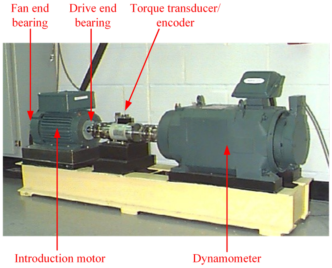
In Case 1, the rolling bearing dataset [34] from Case Western Reserve University (CWRU) is employed to evaluate the performance of the proposed method. Figure 6 shows the experimental rig, which mainly consists of five components: a fan-end bearing, an induction motor, a drive-end bearing, a torque transducer/encoder, and a dynamometer.

In Case 1, the test objects are 6205-2RS JEM deep groove ball bearings manufactured by SKF Group (Gothenburg, Sweden). located at the drive end. The fault types include inner race fault, outer race fault, and ball fault. To simulate different damage levels of rolling bearings, electro-discharge machining (EDM) is applied to process healthy bearings. For each fault type, fault diameters of 0.1778 mm, 0.3556 mm, and 0.5334 mm are introduced.

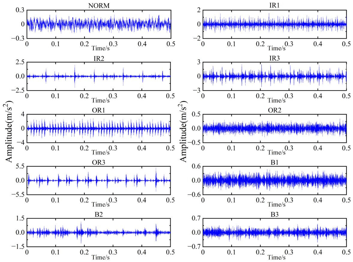
As a result, vibration signals under ten different working conditions are obtained. In this experiment, the motor power is set to 1 HP, the sampling frequency is set to 12 kHz, and the rotational speed is approximately 1772 rpm. For each working condition, 100 non-overlapping samples with a length of 1024 are obtained, among which 20 samples are selected as the training set and the remaining 80 samples as the test set. Therefore, there are 200 training samples and 800 test samples in total. The detailed information of bearings under different working conditions is presented in

Table 2. Description of different working states in Case 1.

Working State	Abbreviation	Fault Diameter (mm)	Training Samples	Test Samples	Label
Normal	NOR	\	20	80	1
Inner race fault 1	IR1	0.1778	20	80	2
Inner race fault 2	IR2	0.3556	20	80	3
Inner race fault 3	IR3	0.5334	20	80	4
Outer race fault 1	OR1	0.1778	20	80	5
Outer race fault 2	OR2	0.3556	20	80	6
Outer race fault 3	OR3	0.5334	20	80	7
Ball fault 1	B1	0.1778	20	80	8
Ball fault 2	B2	0.3556	20	80	9
Ball fault 3	B3	0.5334	20	80	10

, and the corresponding vibration signal waveforms are shown in Figure 7.

After obtaining all signal samples, the MSC index is used to determine the optimal parameter combination $(\delta ,\gamma ,m)$ of ECMSE. To this end, after each random split, the 20 training samples of each working state were used for MSC-based parameter selection, and no test samples were involved in this process. The MSC values of the training samples under different parameters were calculated. To simplify parameter selection, $m=2$ is first fixed to observe the variation in the low threshold $\delta$ under different high thresholds. 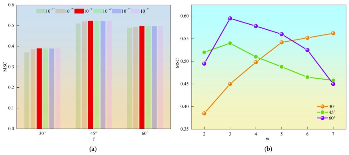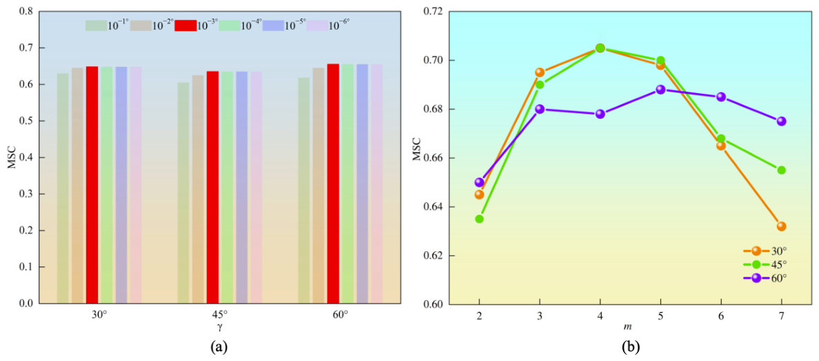Figure 8a shows that as $\delta$ decreases, the MSC values for the three $\gamma$ groups gradually increase. When $\delta$ decreases to ${10}^{-3}$ or lower, the MSC values in each group reach their maximum; therefore, the optimal $\delta$ is set to ${10}^{-3}$. Subsequently, with the optimal low threshold fixed, the MSC values under different combinations $(\gamma ,m)$ are calculated. As shown in Figure 8b, the MSC reaches the maximum value when $\gamma =30°$ and $m=4$. Consequently, the final parameters of ECMSE are set as $m=4$, $\tau =1$, $\delta ={10}^{-3}$, $\gamma =30°$, and $L=1024$. Next, the ECMSE features of all samples are calculated. The feature vectors of the training set are fed into the HBA–KELM classifier for training, and then the feature vectors of the test set are fed into the optimized model for verification. 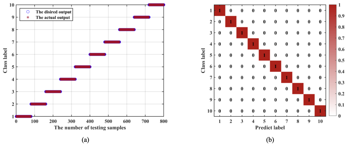As displayed in Figure 9, the proposed approach can effectively identify bearing faults with different types and damage degrees, and the maximum recognition accuracy reaches 100%.

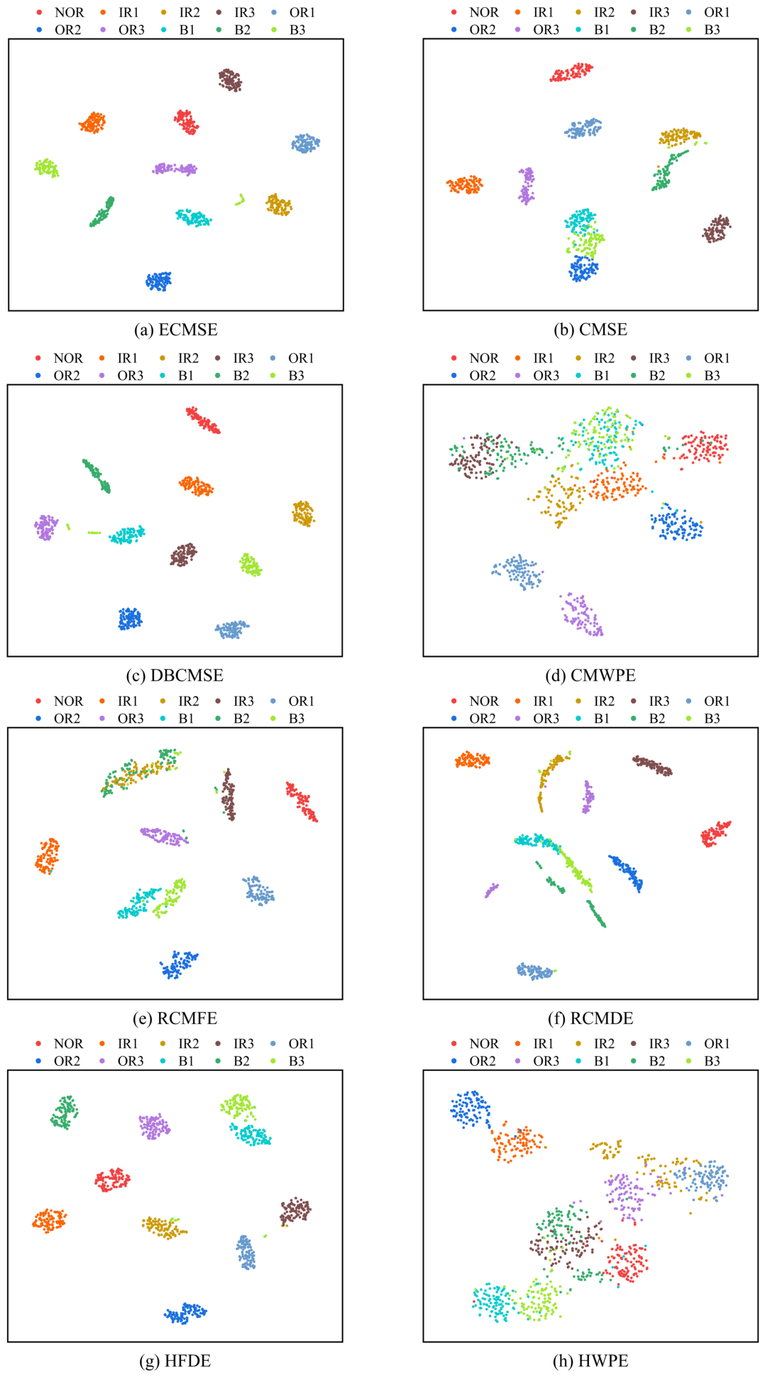
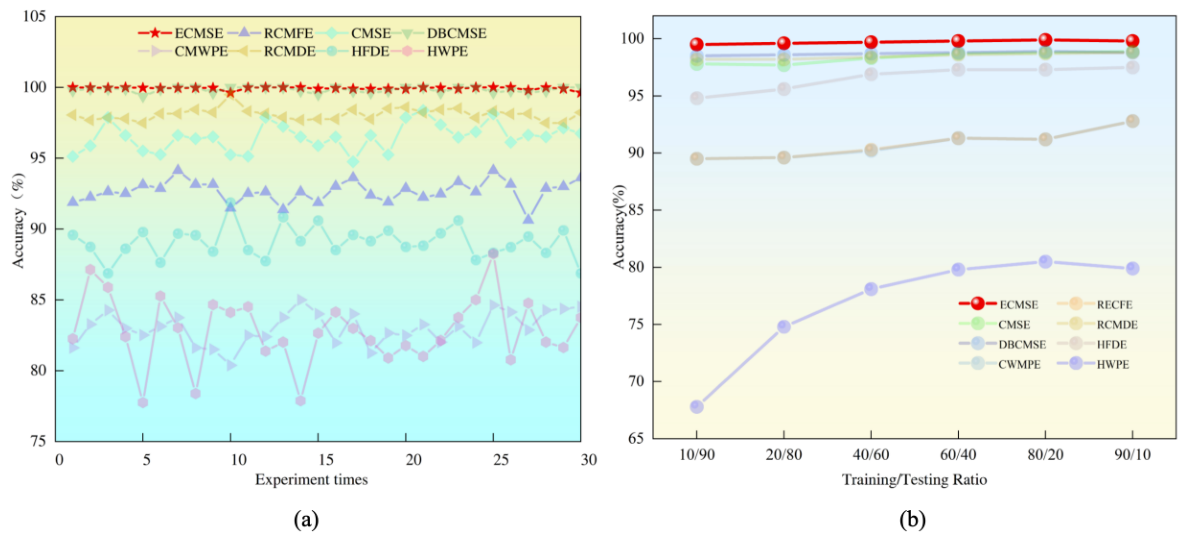
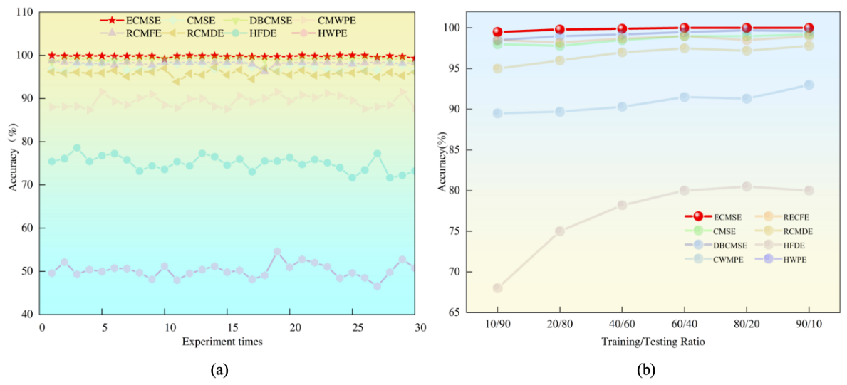
To validate the superiority of the proposed method, feature extraction performance experiments are conducted, and the comparison methods include CMSE, DBCMSE, RCMFE, RCMDE, HFDE, HWPE, and CMWPE. t-SNE [35] is employed to reduce the multidimensional features of all methods to a two-dimensional space, and the visualization results are shown in Figure 10. It can be observed that the inter-class distances of OR2, B1, and B3 in CMSE are too close to be distinguished. In contrast, except for a few misclassified B3 samples, ECMSE and DBCMSE exhibit good separability overall, demonstrating the advantage of the proposed multi-order difference method in extracting detailed information. Additionally, the HFDE method also shows relatively good clustering performance; however, the B1 and B3 faults remain difficult to distinguish. The other methods exhibit issues such as large intra-class dispersion and severe feature overlap, making it difficult to effectively distinguish different fault types. In summary, DBCMSE and ECMSE achieve similar visualization results, with the best clustering performance among all methods. Following feature extraction, the feature vectors are fed into HBA–KELM for classification. To eliminate randomness and ensure reliability, all methods are executed 30 times, with the training and test sets randomly selected before each run. The recognition accuracy and total computation time of different methods are presented in

Table 3. Recognition accuracy and computation time of different methods in Case 1.

Different Methods	Recognition Accuracy (%)				Computing Time (s)
	Max	Min	Mean	SD
ECMSE + HBA −KELM	100	99.63	99.95	0.1	47.098
CMSE + HBA − KELM	98.38	94.75	96.5	0.95	28.336
DBCMSE + HBA − KELM	100	99.38	99.84	0.18	18.592
CMWPE + HBA − KELM	85	80.38	83	1.14	94.958
RCMFE + HBA − KELM	94.13	90.63	92.67	0.76	165.929
RCMDE + HBA − KELM	99.5	97.5	98.06	0.49	47.689
HFDE + HBA − KELM	91.88	86.88	89.06	1.06	29.966
HWPE + HBA − KELM	88.25	77.75	82.80	2.39	28.485

and Figure 11a. As shown, the proposed ECMSE method achieves the highest recognition accuracy in all experiments.

Furthermore, although DBCMSE requires the shortest computation time, the integration of CMSE and DBCMSE in ECMSE increases the computational cost slightly, while significantly improving diagnostic accuracy and robustness.

In addition, to further analyze the influence of sample set partitioning on the experimental results, six scenarios (i.e., training set/test set ratios) are considered: 10/90, 20/80, 40/60, 60/40, 80/20, and 90/10. Figure 11b shows the average recognition accuracy for each scenario over 30 runs. As observed, increasing the size of the training set contributes positively to improving recognition accuracy. However, an excessive number of training samples may reduce the efficiency of classifier parameter optimization. On the other hand, variations in the sample ratio have little effect on the proposed method, and its accuracy reaches the maximum under all conditions. Notably, although DBCMSE performs similarly to ECMSE in Case 1, its classification performance degrades when the training/test ratio is 10/90, indicating that ECMSE is less dependent on the number of training samples. Overall, the proposed method demonstrates clear advantages in both recognition accuracy and robustness.

4.3. Test Verification Case 2

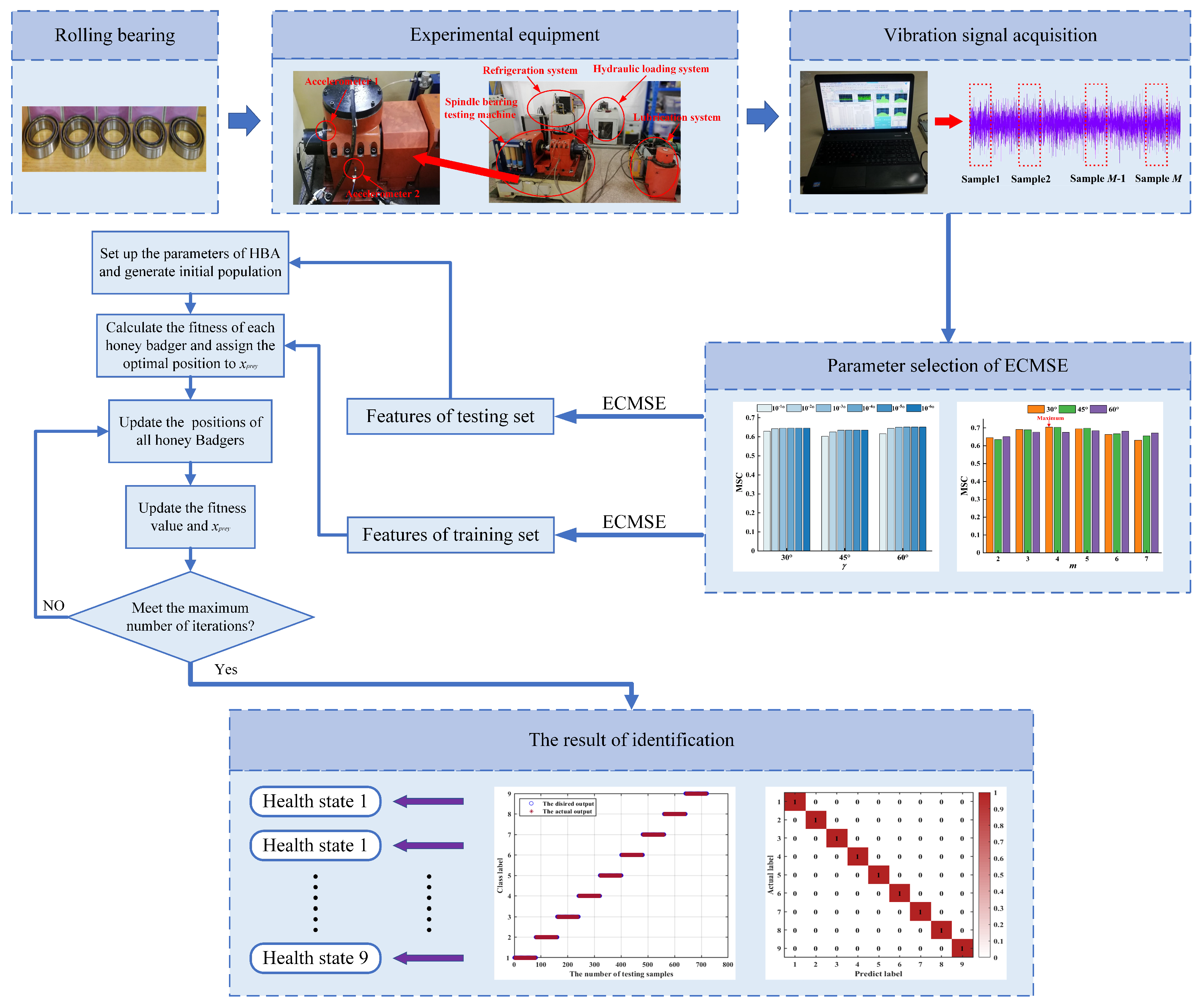
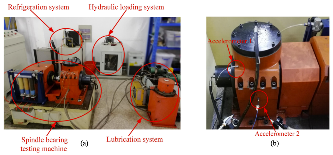
In Case 2, the experimental data were obtained from the aero-engine bearing test bench in the laboratory, which mainly consists of a spindle testing machine, a refrigeration system, a hydraulic loading system, and a lubrication system. Figure 12 shows the experimental setup and the locations of the accelerometers. The test object is the NU1010EM (inner race detachable)/N1010EM (outer race detachable) single-row cylindrical roller bearing manufactured by NSK. The bearing fault types include inner race fault, outer race fault, ball fault, outer race and ball compound fault, and inner race and ball compound fault.

The main geometric parameters of the tested bearing are listed in

Table 4. Main parameters of the tested cylindrical roller bearing in Case 2.

Parameter	Value
Bearing model	NU1010EM/N1010EM
Manufacturer	NSK
Bearing type	Single-row cylindrical roller bearing
Bore diameter	50 mm
Outer diameter	80 mm
Width	16 mm

. Two piezoelectric acceleration sensors were mounted on the bearing housing by threaded connections, as shown in Figure 12b. Accelerometer 1 was installed near the upper radial position of the bearing housing, and Accelerometer 2 was installed near the lower radial position to collect vibration responses from different measurement locations.

To simulate different degrees of bearing damage, a laser marking machine and a wire cutting machine were used to process healthy bearings to obtain single-point and multi-point fault bearings with damage dimensions of 9 mm (length) × 0.2 mm (width). For single-point faults, one rectangular defect was fabricated on the corresponding bearing component. For multi-point and compound faults, three defects with the same nominal size were fabricated on the corresponding single or combined components, as summarized in

Table 5. Description of different working states in Case 2.

Working State	Abbreviation	Fault Size (mm)	Training Samples	Test Samples	Label
Normal	NOR	\	20	80	1
Inner race fault 1	IRF1	9 × 0.2 (1 defect)	20	80	2
Outer race fault 1	ORF1	9 × 0.2 (1 defect)	20	80	3
Ball fault 1	BF1	9 × 0.2 (1 defect)	20	80	4
Outer race and ball compound fault	OBF	9 × 0.2 (3 defects)	20	80	5
Inner race and ball compound fault	IBF	9 × 0.2 (3 defects)	20	80	6
Inner race fault 2	IRF2	9 × 0.2 (3 defects)	20	80	7
Outer race fault 2	ORF2	9 × 0.2 (3 defects)	20	80	8
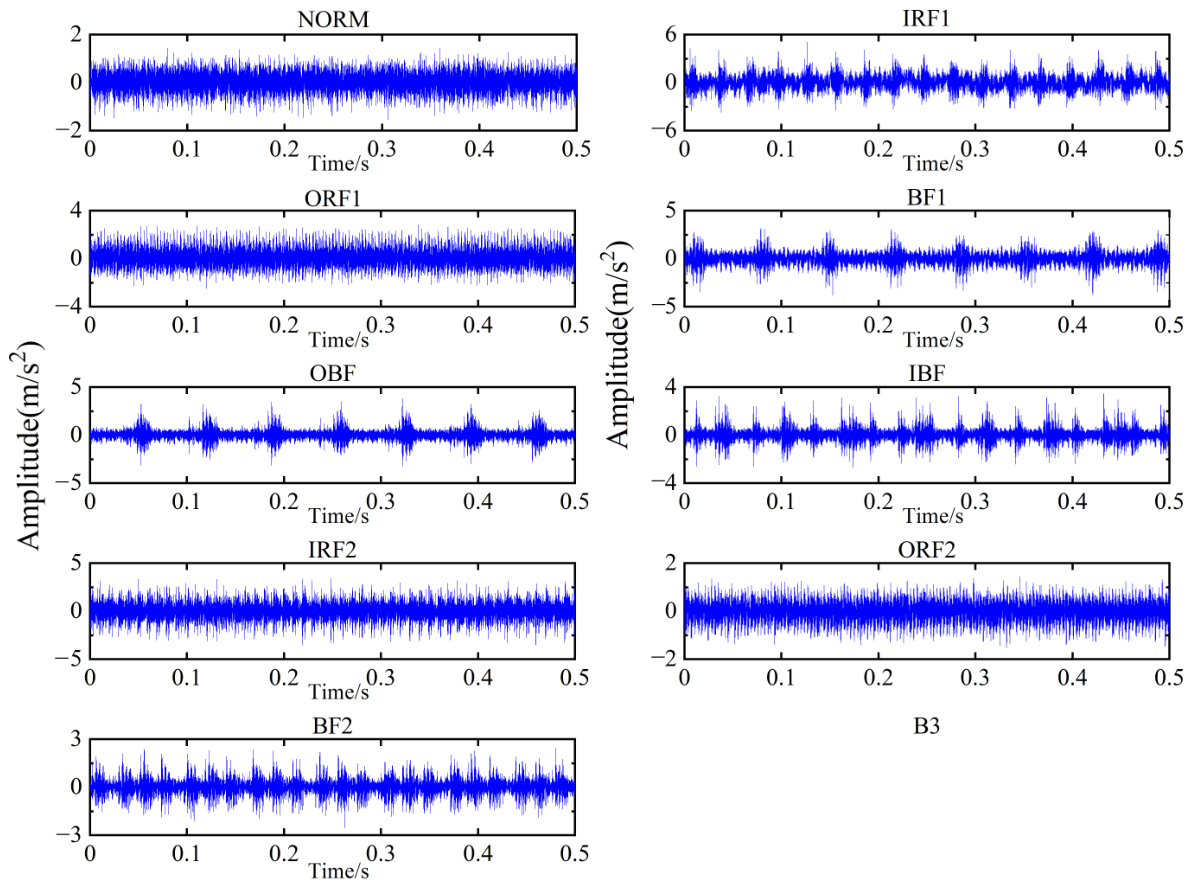
Ball fault 2	BF2	9 × 0.2 (3 defects)	20	80	9

. In Case 2, a total of nine vibration signals of rolling bearings under different working conditions were collected. During the data acquisition process, the axial load was set to 2 kN, the motor speed was set to 2000 rpm, and the sampling frequency was 20.48 kHz. For each working condition, 100 non-overlapping samples were obtained, of which 20 samples were selected as the training set, and the remaining 80 samples were used as the test set. The length of each sample is 1024. The detailed information of bearings under different working conditions is presented in Table 5, and the corresponding waveforms are shown in Figure 13. In this subsection, the parameter selection procedure of ECMSE is the same as that in Case 1. After each random training/test split, the 20 training samples of each bearing type are used for MSC-based parameter selection, and the test samples are not used during parameter tuning. The MSC values of the training samples are calculated under different parameter settings.

Figure 14a shows that as the low threshold $\delta$ decreases, the MSC trends corresponding to different high thresholds $\gamma$ are generally consistent. When $\delta ={10}^{-3}$, the MSC values of the three groups reach their maximum and remain unchanged thereafter. Therefore, the optimal value of $\delta$ is set to ${10}^{-3}$. The selection process of the low threshold in Cases 1 and 2 indicates that even if $\gamma$ varies, the MSC trends with respect to $\delta$ remain similar. Hence, it is feasible to determine $\delta$ independently. Similar to Case 1, the MSC values under different parameter combinations $(\gamma ,m)$ are shown in Figure 14b. It can be observed that the MSC reaches its maximum when $\gamma =60°$ and $m=3$. Accordingly, the final parameters of ECMSE are determined as $m=3$, $\tau =1$, $\delta ={10}^{-3}$, $\gamma =60°$, and $L=1024$. The different optimal parameter combinations selected in Case 1 ($m=4$, $\gamma =30°$) and Case 2 ($m=3$, $\gamma =60°$) reflect the data-dependent sensitivity of ECMSE parameters. The low threshold $\delta$ mainly identifies approximately equal adjacent amplitudes, and its MSC trends are similar in the two cases; once $\delta$ decreases to ${10}^{-3}$, the MSC values become stable, indicating that ECMSE is relatively insensitive to smaller $\delta$ values. By contrast, the high threshold $\gamma$ and embedding dimension m directly affect the symbolic slope patterns and are more sensitive to the signal structure. For the CWRU dataset in Case 1, the single-point faults are characterized by relatively regular impulse responses with subtle amplitude variations, so a lower high threshold and a slightly larger embedding dimension help capture fine local fluctuation patterns. In Case 2, the private dataset differs in bearing type, acquisition platform, and fault form, and the multi-point and compound faults produce more complex amplitude changes; therefore, a larger high threshold and a lower embedding dimension reduce excessive pattern fragmentation and provide better feature separability. This indicates that the optimal ECMSE parameters should be selected according to the target dataset, while the compact MSC-based search range enables stable parameter determination using only the training samples. Subsequently, the ECMSE features of all samples are extracted. The feature vectors of the training set are then fed into the fault classifier for model training, and the feature vectors of the test set are input into the optimized model for fault identification.

Similar to Case 1, the features extracted by all methods are input into HBA–KELM for classification experiments. To avoid randomness and ensure reliability, each method is executed 30 times, with the training and test sets randomly selected each time. The experimental results are presented in

Table 6. Recognition accuracy and computation time of different methods in Case 2.

Different Methods	Recognition Accuracy (%)				Computing Time (s)
	Max	Min	Mean	SD
ECMSE + HBA − KELM	100	99.17	99.82	0.18	42.719
CMSE + HBA − KELM	98.89	96.25	97.78	0.75	25.659
DBCMSE + HBA − KELM	99.58	98.19	99.11	0.32	16.576
CMWPE + HBA − KELM	91.53	87.36	89.40	0.99	45.626
RCMFE + HBA − KELM	98.75	96.25	97.97	0.54	169.540
RCMDE + HBA − KELM	97.22	93.89	95.90	0.73	23.486
HFDE + HBA − KELM	78.61	71.67	75.47	1.47	26.250
HWPE + HBA − KELM	54.58	46.53	50.13	1.76	22.995

and Figure 15a. It can be observed that the proposed method achieves the highest average recognition accuracy and the smallest standard deviation. Additionally, although DBCMSE requires the shortest computation time, its average accuracy is only 99.11%, which is lower than that of ECMSE (99.82%). Furthermore, the training/test sets are divided into different ratios (10/90, 20/80, 40/60, 60/40, 80/20, and 90/10). The average recognition accuracy is calculated over 30 runs for each ratio, and the results are shown in Figure 15b. The recognition accuracy of the comparative methods remains below that of the proposed method under all training/test ratios, further demonstrating the superiority of ECMSE.

4.4. Additional Robustness and Baseline Analysis

To further address the robustness and baseline concerns, three additional analyses are conducted: (1) an SNR-based noise robustness test, (2) a comparison with representative 1D signal-based machine-learning and deep-learning baselines, and (3) a classifier optimization ablation study. For the noise robustness test, additive white Gaussian noise is injected into the Case 1 test samples at different SNR levels, while the training samples remain unchanged. Each method is repeated 30 times under the same random partitions. The results are shown in

Table 7. Noise robustness results for Case 1 under different SNR levels.

Method	Recognition Accuracy (%, Mean ± SD)
	Clean	12 dB	8 dB	4 dB	0 dB	−4 dB
ECMSE + HBA − KELM	99.95 ± 0.10	99.70 ± 0.16	99.31 ± 0.24	98.42 ± 0.37	96.53 ± 0.62	93.68 ± 0.91
DBCMSE + HBA − KELM	99.84 ± 0.18	99.20 ± 0.22	98.76 ± 0.31	97.31 ± 0.48	94.80 ± 0.74	90.45 ± 1.10
CMSE + HBA − KELM	96.50 ± 0.95	95.82 ± 1.02	94.18 ± 1.16	91.72 ± 1.41	86.54 ± 1.86	80.33 ± 2.24
RCMDE + HBA − KELM	98.06 ± 0.49	97.38 ± 0.58	96.42 ± 0.73	93.85 ± 0.96	89.76 ± 1.33	84.62 ± 1.71
RCMFE + HBA − KELM	92.67 ± 0.76	91.85 ± 0.88	90.24 ± 1.05	87.36 ± 1.42	82.15 ± 1.93	76.54 ± 2.35

.

It is worth emphasizing that ECMSE exhibits the best anti-noise performance among all compared methods, highlighting its engineering applicability in noisy bearing monitoring environments. Even under the severe $-4$ dB condition, ECMSE still achieves an average recognition accuracy of 93.68%, outperforming DBCMSE, CMSE, RCMDE, and RCMFE by 3.23, 13.35, 9.06, and 17.14 percentage points, respectively.

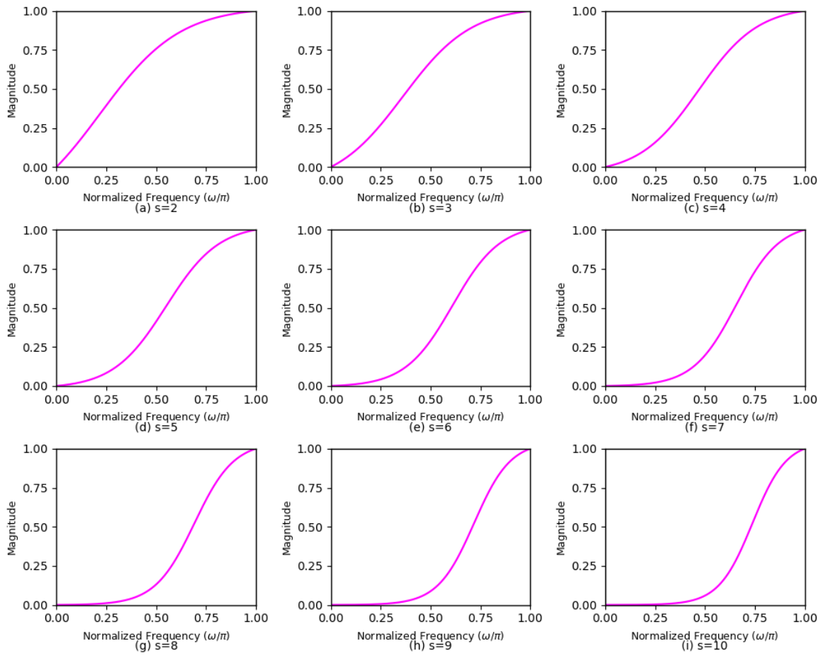
As shown in Table 7, the recognition accuracy of all methods decreases as the noise intensity increases, but ECMSE maintains the highest average accuracy at all SNR levels. When the SNR decreases from the clean condition to $-4$ dB, the accuracy of ECMSE decreases by 6.27 percentage points, which is smaller than the decreases of DBCMSE (9.39 percentage points), CMSE (16.17 percentage points), RCMDE (13.44 percentage points), and RCMFE (16.13 percentage points). These results indicate that the fusion of CMSE and DBCMSE improves robustness under noisy conditions: the CMSE branch retains relatively stable low-frequency trend information, while the DBCMSE branch preserves high-frequency fault-related details.

To position the proposed method against broader fault diagnosis models, representative 1D signal-based baselines are considered, including SVM, KELM, 1D-CNN, CNN-LSTM, and 1D-ResNet. For a fair comparison, all additional baselines use the same training/test partitions as the entropy-based methods, and the test samples are not used for model selection. The comparison results are shown in

Table 8. Comparison with representative machine-learning and deep-learning baselines.

Method	Input Type	Case 1 Accuracy (%)	Case 2 Accuracy (%)
SVM	Raw signal	94.62 ± 1.21	92.48 ± 1.46
KELM	Raw signal	95.38 ± 0.98	93.76 ± 1.22
1D-CNN	Raw signal	98.72 ± 0.41	97.93 ± 0.62
CNN-LSTM	Raw signal	98.91 ± 0.38	98.24 ± 0.54
1D-ResNet	Raw signal	99.08 ± 0.32	98.61 ± 0.48
ECMSE+HBA–KELM	Entropy features	99.95 ± 0.10	99.82 ± 0.18

.

The results in Table 8 indicate that the proposed ECMSE+HBA–KELM framework achieves competitive performance compared with representative deep-learning models while using compact entropy features and a shallow classifier. In Case 1, ECMSE+HBA–KELM improves the average accuracy by 0.87 percentage points over 1D-ResNet, the strongest deep-learning baseline. In Case 2, the corresponding improvement is 1.21 percentage points. This suggests that the proposed entropy representation remains effective in small-sample diagnosis, where end-to-end deep models may not fully exploit their representation capacity.

To separate the contribution of ECMSE from the classifier optimizer, a classifier ablation study is further conducted by combining ECMSE with KELM, PSO-KELM, GA-KELM, and HBA–KELM. The results are shown in

Table 9. Classifier optimization ablation using ECMSE features.

Classifier	Case 1 Accuracy (%)	Case 2 Accuracy (%)
ECMSE + KELM	98.84 ± 0.36	98.32 ± 0.44
ECMSE + PSO − KELM	99.42 ± 0.22	99.05 ± 0.31
ECMSE + GA − KELM	99.31 ± 0.28	98.96 ± 0.36
ECMSE + HBA − KELM	99.95 ± 0.10	99.82 ± 0.18

.

Finally, to examine whether the improvement of ECMSE over its two branches is statistically meaningful, a paired Wilcoxon signed-rank test is conducted over the 30 repeated runs. In each run, the compared methods use the same random training/test partition, so their recognition accuracies form paired observations. The null hypothesis is that the median paired accuracy difference is zero, and a two-sided test with a significance level of 0.05 is adopted. The statistical results are listed in

Table 10. Statistical significance analysis over 30 runs.

Comparison	Case 1 p-Value	Case 2 p-Value
ECMSE vs. CMSE	<0.001	<0.001
ECMSE vs. DBCMSE	0.018	0.003
ECMSE vs. RCMDE	<0.001	<0.001

.

The ablation results in Table 9 show that HBA–KELM provides the best classification performance among the tested KELM variants. Compared with ECMSE + KELM, ECMSE + HBA − KELM improves the mean accuracy by 1.11 percentage points in Case 1 and 1.50 percentage points in Case 2. It also outperforms ECMSE+PSO-KELM and ECMSE+GA-KELM, indicating that HBA is effective for optimizing the KELM parameters in this task. In addition, Table 10 shows that the improvement of ECMSE over CMSE and RCMDE is highly significant in both cases. The improvement over DBCMSE is smaller but still statistically significant, with $p=0.018$ in Case 1 and $p=0.003$ in Case 2. These results support the effectiveness of fusing the low-frequency CMSE branch and the high-frequency DBCMSE branch.

5. Conclusions

To accurately identify different fault types of rolling bearings, an intelligent fault diagnosis method based on ECMSE and HBA–KELM is proposed in this paper. In the feature extraction stage, the CMSE method is employed to capture low-frequency information from time series, while a multi-order difference strategy is introduced to construct the DBCMSE method for extracting high-frequency information. By integrating these two approaches, ECMSE is developed to effectively extract comprehensive fault features of rolling bearings. Subsequently, the MSC criterion is utilized to determine the optimal parameter combination of ECMSE. In the fault identification stage, HBA is used to optimize the regularization parameter and kernel parameter of KELM, thereby establishing an effective fault diagnosis model. Experimental results on two datasets demonstrate that the proposed method can accurately identify different fault types and damage severities of rolling bearings, as well as effectively distinguish composite faults. Furthermore, comparative experiments verify that ECMSE achieves superior feature extraction capability, higher recognition accuracy, and better stability than existing methods. Although the two datasets used in this study include different bearing types, fault categories, and acquisition platforms, the current validation is still limited to fixed operating conditions. More challenging scenarios, such as variable speeds, variable loads, non-Gaussian noise, and cross-domain transfer between different machines, should be further investigated. Future work will focus on applying the proposed method to fault diagnosis of other rotating machinery and further investigating its performance under variable operating conditions.