Article

Generalized AUC Maximization Core Vector Machine: A Multi-Kernel Learning Approach for Fast Imbalanced Classification

1
The Internet of Things Engineering College, Jiangsu Vocational College of Information Technology, Wuxi 214153, China
2
School of Artificial Intelligence and Computer Science, Jiangnan University, Wuxi 214122, China
3
School of Medical Information and Engineering, Bengbu Medical University, Bengbu 233030, China
*
Author to whom correspondence should be addressed.
Electronics 2026, 15(10), 2228; https://doi.org/10.3390/electronics15102228
Submission received: 12 April 2026 / Revised: 16 May 2026 / Accepted: 18 May 2026 / Published: 21 May 2026
(This article belongs to the Special Issue Multimodal Learning for Multimedia Content Analysis and Understanding)

Abstract

Imbalanced classification remains a fundamental challenge in machine learning, where the Area Under the ROC Curve (AUC) is widely used for threshold-independent ranking evaluation, especially in AUC maximization studies. Existing AUC maximization methods suffer from two critical limitations: they rely on single fixed kernels that fail to capture complex data structures, and they incur prohibitive computational costs due to pairwise constraint construction. To address these issues, we propose the Generalized AUC Maximization Core Vector Machine (GAM-CVM), a fast imbalanced classification framework integrating multi-kernel learning with core vector machine optimization. Multiple affinity graphs are constructed from complementary perspectives and fused via cross-diffusion into a unified kernel matrix that respects the intrinsic data manifold. This fused kernel is embedded into a generalized AUC objective with a flexible ranking margin. Given the fused kernel matrix, the optimization stage of GAM-CVM achieves asymptotic linear time complexity with respect to the number of sample pairs under a fixed approximation accuracy by reformulating the learning objective as a center-constrained minimum enclosing ball problem. Extensive experiments demonstrate that GAM-CVM achieves the best overall average ranking and significantly outperforms most competing methods while maintaining the lowest optimization-stage running time.

1. Introduction

Imbalanced classification remains a persistent challenge in machine learning, particularly in applications where minority classes carry disproportionate importance. For example, in medical diagnosis, the number of patients with a rare disease is typically far smaller than that of healthy individuals, yet misdiagnosing a patient can have life-threatening consequences, whereas false positives often entail comparatively lower clinical risk [1]. This inherent asymmetry between class distributions poses significant difficulties for conventional classification algorithms. Standard methods such as support vector machines, neural networks, and decision trees are designed under the assumption of balanced class distributions and, consequently, tend to favor the majority class when confronted with imbalanced data [2]. These methods achieve high overall accuracy by correctly classifying most majority instances while failing to identify minority class instances that often carry the most critical information. Various strategies have been developed to address this issue, including resampling techniques that balance class distributions through oversampling or undersampling [3,4], cost-sensitive learning that assigns higher misclassification costs to minority samples [5], and ensemble methods that combine multiple classifiers to improve minority class recognition [6]. Despite these efforts, direct optimization of class-imbalance-aware metrics offers a theoretically grounded alternative to heuristic resampling or reweighting strategies.
The receiver operating characteristic (ROC) curve and the area under the ROC curve (AUC) are widely used in imbalanced classification, particularly when the goal is to evaluate the ranking quality of a scoring function [7]. From the Wilcoxon–Mann–Whitney perspective, AUC measures the probability that a randomly selected positive sample is ranked above a randomly selected negative sample. This pairwise interpretation makes AUC especially suitable for ranking-oriented learning problems and has motivated a large body of AUC maximization methods [8]. Early work by Brefeld and Scheffer proposed the AUC maximizing support vector machine (AUCSVM), which formulated AUC optimization as a pairwise learning problem and demonstrated superior performance on imbalanced datasets [9]. Following this direction, various extensions have been developed, including online AUC maximization methods that enable efficient learning from streaming data [10,11], and stochastic AUC maximization approaches that achieve favorable convergence rates [12,13]. For large-scale nonlinear settings, Dang et al. proposed a triply stochastic gradient method (TSAM) that approximates kernel functions using random Fourier features, enabling scalable AUC optimization on massive datasets [14]. Wang et al. also developed an extreme learning machine based on the AUC maximization framework (AUC-ELM) for supervised and semi-supervised imbalanced binary classification [15].
Nevertheless, most existing AUC maximization methods are constrained by two interrelated issues: limited representational capacity of the similarity measure and prohibitive computational cost. The first concerns the representational capacity of similarity measures. Most approaches construct pairwise relationships using some single fixed kernels, such as linear kernel or Gaussian kernel, which fail to capture complex data distributions. Pairwise ranking depends not only on Euclidean proximity but also on local density, feature correlation, and manifold geometry. Relying on a single kernel of similarity overlooks complementary information that could substantially improve ranking performance. Moreover, the standard AUC metric treats all samples equally, which may not reflect the importance of minority classes or the presence of noise [16]. The second limitation concerns computational efficiency. With positive and negative samples, the number of pairwise constraints equals their product, leading to quadratic growth in complexity and memory. For datasets with thousands or millions of samples, this scaling becomes prohibitive. While approximate methods such as stochastic gradients have been proposed to alleviate this bottleneck [12,13], they often sacrifice solution quality or introduce additional hyperparameters. A principled approach that maintains accuracy while achieving near-linear scalability remains highly desirable.
Recently, two strategies have been explored to enhance the representational flexibility of AUC maximization. The first generalizes the AUC concept by introducing a flexible ranking margin that emphasizes the importance of minority classes [17]. The second explores multi-kernel learning, which captures complementary information from diverse data representations. Recent advances demonstrate that integrating multiple kernels can substantially improve similarity representations by respecting intrinsic data manifold structures [18,19]. Techniques such as cross-diffusion for metric fusion and ensemble clustering have shown the potential of multi-kernel approaches [20,21]. These developments suggest that multi-kernel fusion could benefit AUC maximization by constructing more informative similarity measures between sample pairs.
To address the second limitation concerning computational efficiency, core vector machine (CVM) techniques offer an effective route to mitigate the computational bottleneck of pairwise AUC optimization [22]. By reformulating support vector machine optimization as a minimum enclosing ball problem, the core vector machine achieves asymptotic linear time complexity with respect to the number of training samples while maintaining constant space complexity through the use of core sets. Tsang et al. demonstrated that this approach can scale to millions of samples without significant loss in accuracy [23]. CVM methods exploit the fact that the optimal solution can be determined from a small core set of representative samples. This core set approximation provides a principled way to achieve near-linear scalability while preserving theoretical convergence guarantees. More recently, extensions of core vector machines to distributionally robust optimization and large-scale clustering have further validated the effectiveness of core set methods for scalable machine learning [24,25].
In this work, we propose the Generalized AUC Maximization Core Vector Machine (GAM-CVM), which combines multi-kernel fusion with core set-based optimization for fast imbalanced classification. GAM-CVM departs from single-kernel formulations by constructing affinity graphs from multiple complementary sub-kernels and fusing them via cross-diffusion into a unified kernel that preserves the intrinsic data manifold. This fused kernel is then embedded into a generalized AUC objective with a flexible ranking margin. By reformulating the optimization as a center-constrained minimum enclosing ball (CCMEB) problem, the core vector machine technique enables the optimization stage of GAM-CVM to achieve asymptotic linear time complexity with respect to the number of sample pairs under a given fused affinity matrix and fixed approximation accuracy. Nevertheless, the area under the ROC curve is not a universally sufficient metric for all imbalanced learning scenarios. When the main objective is to ensure high precision of positive predictions under a specific operating threshold, precision-recall-oriented metrics such as area under the precision-recall curve or average precision may provide complementary information. In this work, we focus on scalable AUC maximization because our objective, constraints, and CCMEB reformulation are all built upon positive–negative pairwise ranking. The contributions of this work can be summarized as follows:
(1)
We first propose a generalized AUC objective that incorporates a flexible ranking margin, which enforces stricter separation between classes and naturally emphasizes the importance of minority samples.
(2)
Second, we develop a multi-kernel learning procedure in which complementary affinity graphs are integrated via cross-diffusion to form a unified kernel that captures diverse similarity cues.
(3)
Third, by reformulating the resulting optimization as a center-constrained minimum enclosing ball problem, we apply the core vector machine technique to achieve linear time complexity in the number of sample pairs under a given fused affinity matrix and fixed approximation accuracy.
The remainder of this paper is organized as follows: Section 2 formulates the generalized AUC objective. Section 3 describes the multi-kernel fusion strategy. Section 4 presents the core vector machine-based training algorithm. Section 5 reports experimental results, and Section 6 concludes with a discussion of future directions.

2. Generalized AUC Maximization Learning

In this section, we first introduce the generalized AUC metric, which extends the conventional AUC by incorporating a flexible ranking margin to better capture the importance of minority classes. We then present the generalized AUC maximization learning model, which formulates the optimization objective for imbalanced classification.

2.1. The Generalized AUC Metric

For a binary classifier f ( · ) , given the random variables X + ~ P + of positive samples and X ~ P of negative samples, the classical AUC metric can be defined as
A U C ( f ) = E X + ~ P + , X ~ P ( I ( f X + > f ( X ) ) ) ,
where I ( · ) is the indicator function
I f X + > f X = 1 ,       i f   f X + > f X   0 ,       e l s e .
According to the normalized Wilcoxon–Mann–Whitney statistic [26], given n + positive samples x i + ( i = 1 , 2 , , n + ) that follow P + and n negative samples x j ( j = 1 , 2 , , n ) that follow P , the maximum likelihood estimate of the classical AUC metric can be given as
A U C ^ ( f ) = 1 n + n i = 1 n + j = 1 n I ( f x i + > f x j ) .
As is well known, for most kernel methods, the classifier f ( · ) can be represented as f x = ω , φ x + b , where any sample x = ( x 1 , x 2 , , x d ) x | x = x i +   o r   x = x j has d features, ω is the weight vector, b is a constant and φ ( · ) is the mapping function [27]. Actually, φ ( · ) denotes an implicit preprocessing of the input features, which is equivalent to mapping the sample space P + P into some feature space. In many practical scenarios, φ ( · ) may map the input features to infinite dimensions, hence the kernel function k x , y = φ ( x ) , φ ( y ) is usually adopted instead of giving the exact form of φ ( x ) . Please note that the metric A U C ^ ( f ) is independent of the constant term b ; we can simplify the classifier as f x = ω , φ x in the rest of this work.
Since the AUC metric in Equation (3) depends only on the ranking of each sample by the classifier, it exhibits strong robustness in imbalanced binary classification tasks. However, taking into account the potential influence of noise in real-world data, and with the aim of emphasizing the significance of the minority class, we introduce a flexible ranking margin τ to generalize the definition of A U C ^ ( f ) . The generalized AUC metric g A U C ^ ( f ) can be defined by expanding the margin between positive and negative sample pairs:
g A U C ^ f = 1 n + n i = 1 n + j = 1 n I ( f x i + > f x j + τ ) .
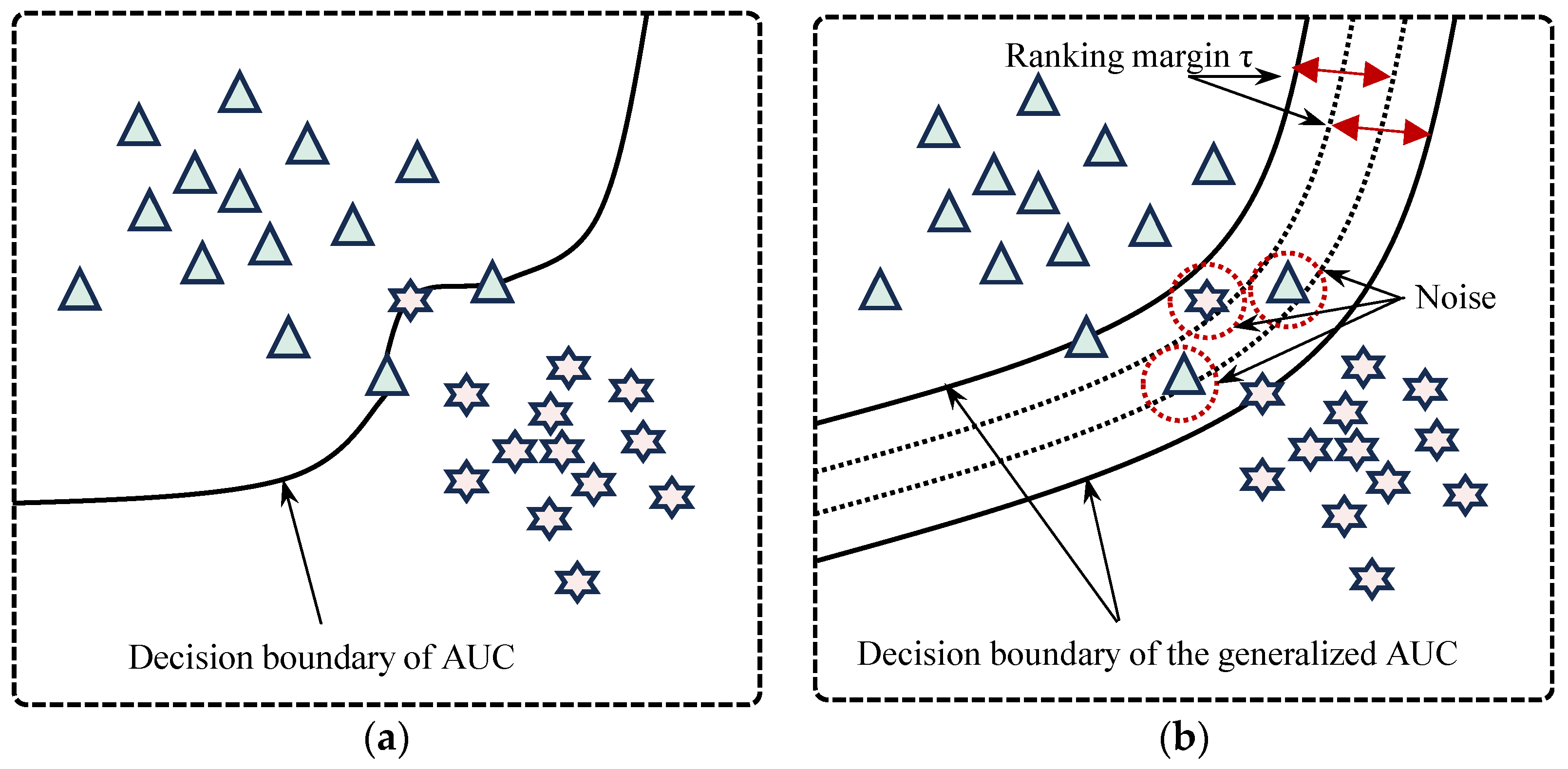
In fact, when the given dataset is contaminated with noise, the introduction of the flexible ranking margin τ significantly enhances the robustness of the AUC metric. In a sense, τ reflects the upper bound of the classifier’s tolerance to the potential noise. Figure 1 contrasts the decision boundaries of standard AUC maximization and the proposed generalized AUC formulation under noisy conditions. The ranking margin τ in the generalized objective reduces sensitivity to outliers by enforcing a more conservative class separation. As illustrated, the generalized approach not only produces a more robust decision boundary but also automatically detects noisy samples, which can be flagged for further inspection.

2.2. Learning Objective of the Generalized AUC Maximization

Similar to AUC maximization learning methods [9,17], our core idea is to optimize the generalized AUC metric g A U C ^ ( f ) directly as the learning objective. Unfortunately, due to the presence of the indicator function I ( · ) , the problem of directly maximizing Equation (4) is clearly non-convex and thus difficult to solve. Practically, the generalized AUC metric g A U C ^ ( f ) depends on the number of sample pairs x i + , x j that satisfy the following constraints:
ω , φ x i + ω , φ x j τ > 0 .
If a geometrical margin γ = γ ~ / ω is introduced as confidence measure of maximizing the AUC metric, the hard margin learning model can be expressed as
max ω   γ ,
s .   t .   ω , φ x i + ω , φ x j > γ ~ ,     i = 1 , 2 , , n + ,     j = 1 , 2 , , n ,
where the geometrical margin γ is maximized by fixing functional margin γ ~ = 1 and minimizing the norm of ω according to the existing AUC maximization methods [9,17]. Let the hyperparameter C 1 > 0 and the slack variable for any sample pair θ i j 0 , then the soft AUC maximization can be solved by
min ω , θ ij 1 2 ω 2 + C 1 2 i , j θ i j 2 ,
s .   t .   ω , φ x i + ω , φ x j > 1 θ i j ,   i = 1 , 2 , , n + ,     j = 1 , 2 , , n ,
θ i j 0 ,     i = 1 , 2 , , n + ,     j = 1 , 2 , , n .
Please note that, unlike the existing AUC maximization methods, the functional margin for the generalized AUC maximization learning is no longer fixed at 1 and can be replaced by the flexible ranking margin τ . It is obvious that for the optimization problem in Equations (6)–(10), maximizing γ is equivalent to minimizing ω 2 and maximizing the flexible ranking margin τ . Assume that C 2 > 0 is another user-defined regularization hyperparameter, then the learning objective of the generalized AUC maximization can be expressed as
min ω , θ ij , τ 1 2 ω 2 + C 1 2 i , j θ i j 2 C 2 τ ,
s .   t .   ω , φ x i + ω , φ x j > τ θ i j ,   i = 1 , 2 , , n + ,     j = 1 , 2 , , n ,
θ i j 0 ,     i = 1 , 2 , , n + ,     j = 1 , 2 , , n .
In summary, the objective in Equations (11)–(13) is convex and can be solved via standard quadratic programming, thanks to the introduction of the flexible margin τ , which improves robustness to noise and highlights the minority class. Nevertheless, the pairwise formulation introduces n + n constraints, leading to quadratic growth in both time and memory, which is a critical bottleneck for medium to large datasets.

3. Multi-Kernel Learning

The learning objective presented in Section 2 assumes a predefined kernel. Most existing AUC maximization methods adopt a single fixed kernel, e.g., typically Gaussian or linear, to evaluate pairwise similarities. This single-kernel strategy imposes strong assumptions on the underlying data distribution and often fails to capture the multifaceted nature of complex real-world data, where the likelihood of correct ranking between positive and negative samples may depend on multiple factors beyond Euclidean distance. To overcome this limitation, we propose a multi-kernel learning framework that constructs multiple complementary kernels and fuses them into a unified representation. This section details the definition of multi-kernel and the cross-diffusion-based fusion technique.

3.1. The Definition of Multi-Kernel

In conventional kernel-based AUC maximization, a single kernel function k x i , x j = φ ( x i ) , φ ( x j ) ( i , j = 1 , 2 , ,   ( n + + n ) ) is used to evaluate the similarity between any two samples. The final decision function is then expressed as f x = ω , φ ( ω ) . For a dataset containing n = n + + n samples, the kernel matrix K R n × n is defined with entries K i j = k x i , x j . Different from such a single kernel, we define a multi-kernel as a collection of sub-kernel matrices K ( 1 ) , K ( 2 ) , , K ( M ) , where each sub-kernel K ( m ) ( m = 1 , 2 , , M ) is constructed from a distinct similarity perspective. All the M kernel matrices share the same set of samples but capture complementary aspects of the data distribution.
Without loss of generality, this study mainly employs three representative sub-kernels for experimental validation, while the framework naturally extends to an arbitrary number of sub-kernels. The first sub-kernel is the widely used Gaussian kernel, which measures similarity based on Euclidean distance. Any element K i j ( 1 ) in the Gaussian kernel matrix K ( 1 ) can be defined as
K i j ( 1 ) = e x p ( x i x j 2 2 σ 1 2 ) ,
where σ 1 is the bandwidth parameter, which can be simply set as the median standard deviation of all samples. The Gaussian kernel is sensitive to local proximity and works well when samples of the same class form compact clusters.
The second sub-kernel is based on the Pearson correlation coefficient, which captures linear dependencies that are often more informative than Euclidean distance in high-dimensional settings. Any element K i j ( 2 ) in the Pearson correlation coefficient-based kernel matrix K ( 2 ) can be defined as
K i j ( 2 ) = C o v x i , x j + V a r ( x i ) V a r ( x j ) 2 V a r ( x i ) V a r ( x j ) ,
where C o v x i , x j denotes the covariance between x i and x j , and V a r ( x i ) is the variance of x i . This kernel emphasizes samples that are linearly correlated, which may be missed by distance-based measures.
The third sub-kernel is based on local density, which helps to prevent erroneous label propagation near decision boundaries where samples from different classes may be spatially close. We first compute the local sparsity S P A L o c of each sample x i as
S P A l o c ( x i ) = 1 n l o c l = 1 n l o c D ( l ) ( x i ) ,
where D ( l ) ( x i ) represents the Euclidean distance between x i and the l -th sample closest to x i , and n l o c is a user-given hyperparameter, which is adopted to control the size of the local neighborhood. Then any element K i j ( 3 ) in the density-based kernel matrix K ( 3 ) can be defined as
K i j ( 3 ) = e x p ( ( S P A l o c x i S P A l o c ( x j ) ) 2 2 σ 2 2 ) ,
where the bandwidth parameter σ 2 can be set as the median local sparsity of all samples. The density-based kernel matrix K ( 3 ) encourages propagation between samples with similar local densities and suppresses propagation across density gaps, thus improving robustness to outliers and noise.
The above three sub-kernels are complementary: the Gaussian kernel captures local proximity, the correlation kernel captures global linear dependence, and the density kernel captures structural regularity. By integrating them, we obtain a more comprehensive characterization of sample relationships than any single kernel can provide. It should be emphasized that the proposed multi-kernel framework is not limited to the above three sub-kernels; they are presented here only as representative examples to demonstrate the feasibility of the approach, and more sub-kernels can be incorporated according to specific application scenarios.

3.2. Multi-Kernel Fusion Based on Cross-Diffusion

Once multiple kernel matrices K ( m ) are constructed, the next challenge is to fuse them into a single unified kernel matrix that preserves the complementary information from all sub-kernels. Simply averaging the matrices may dilute the distinct contributions of each sub-kernel. Instead, we adopt a cross-diffusion fusion technique [20], which iteratively diffuses information across different sub-kernels while maintaining local affinity structures.
For m = 1 , 2 , , M , we first normalize the sub-kernel matrix to obtain the corresponding natural kernel matrix K ¯ ( m ) , where any element can be expressed as
K ¯ i j ( m ) = K i j ( m ) m = 1 M K i j ( m ) ,
such that m = 1 M K ¯ i j ( m ) = 1 . This matrix captures full similarity information from the m -th sub-kernel. In parallel, we construct a local kernel matrix L ¯ ( m ) that only retains affinities to the nearest neighbors, reflecting the manifold assumption that label information propagates primarily along local neighborhoods. Specifically, we first construct the sparse kernel matrix L ( m ) by setting any element as
L i j ( m ) = K i j m ,       i f   x j K N N ( x i )   0 ,       e l s e ,
where K N N ( x i ) denotes the set of n l o c (the same as that in Equation (16)) nearest neighbors of x i . Then any element in the local kernel matrix L ¯ ( m ) is defined as
L ¯ i j ( m ) = L i j ( m ) m = 1 M L i j ( m ) .
The cross-diffusion process iteratively updates the status matrices by exchanging information across sub-kernels. To avoid ambiguity, we distinguish the fixed local kernel matrix used for diffusion from the iteratively updated status matrix. Let K ¯ t ( m ) denote the natural kernel matrix of K ¯ ( m ) at iteration t = 1 , 2 , , T , and the update rule is
K ¯ t + 1 ( m ) = L ¯ ( m ) · 1 M 1 s = 1 , s m M K ¯ t ( s ) · L ¯ ( m ) + ρ E ,
where E is the n × n identity matrix and ρ > 0 is the regularization coefficient. Note that both K ¯ t ( m ) and L ¯ ( m ) are generally asymmetric. This update diffuses the status information from other sub-kernels through the local kernel L ¯ ( m ) . After a sufficient number of iterations T , the final fused kernel matrix K ~ is obtained as the average of the converged status matrices and their transposes to enforce symmetry:
K ~ = 1 M m = 1 M 1 2 ( K ¯ T m + ( K ¯ T m ) ) .
The resulting final fused kernel matrix K ~ is a symmetric and non-negative matrix that integrates the complementary information from all M sub-kernels. Actually, the final fused kernel matrix K ~ can serve as the basis for the proposed kernel method, i.e., the generalized AUC maximization in Equations (11)–(13). Subsequently, we provide the convergence proof of the cross-diffusion fusion technique (Equation (21)) in the form of a theorem.
Theorem 1. 
The distance between any two natural kernel matrices  K ¯ t m  and  K ¯ t s  ( m , s 1 , 2 , , M ,  m s ) converges with  t .
Proof of Theorem 1. 
Let the number of sub-kernels be M 2 , and define the distance between any two natural kernel matrices as d K ¯ t m , K ¯ t s = K ¯ t m K ¯ t s F , where · F denotes the Frobenius norm. Since the constant regularization term ρ E does not affect the convergence of the distance, we consider the simplified fusion iteration without it, i.e.,
K ¯ t + 1 ( m ) = L ¯ ( m ) 1 M 1 s m K ¯ t ( s ) L ¯ ( m ) .
Consider one complete round of updating all M sub-kernels. For an arbitrary index m , after one full cycle, the update can be expressed as
( M 1 ) K ¯ M t + 1 m = L ¯ m ( L ¯ M L ¯ 1 ) t s m K ¯ t ( s ) ( L ¯ 1 L ¯ M ) t L ¯ ( m ) .
Let λ 1 , λ 2 , , λ n be the eigenvalues of L ¯ M L ¯ 1 , ordered such that λ 1 λ 2 λ n . By the Perron–Frobenius theorem [28], we have
( L ¯ M L ¯ 1 ) t = 1 π + O ( n m 2 1 λ 2 t ) ,
where 1 is the all-ones column vector, π is the dominant left eigenvector (stationary distribution), and m 2 is the algebraic multiplicity of λ 2 . As t , for any matrix B , we have
( L ¯ M L ¯ 1 ) t B ( L ¯ 1 L ¯ M ) t Φ ,
where Φ is a fixed matrix that depends only on π . Consequently, for any two distinct m and s , the natural kernel matrices K ¯ t m and K ¯ t s converge to the same fixed matrix up to a constant transformation. Hence, the distances satisfy
lim t K ¯ t m K ¯ t s F = Φ L ¯ 1 Φ L ¯ 1 F = ϵ m , s ,
where ϵ m , s is a constant. Thus, the distances between any two natural kernel matrices converge, completing the proof. □
As noted earlier, the kernel used in existing AUC maximization methods is typically a single fixed kernel, which may not capture the diverse similarity patterns in real-world data. These limitations motivate the introduction of multi-kernel learning, which not only enriches the representation of sample relationships but also facilitates subsequent optimization via core vector machine techniques, as detailed in the following sections.

4. Generalized AUC Maximization Core Vector Machine for Fast Imbalanced Classification

In this section, we present the proposed Generalized AUC Maximization Core Vector Machine (GAM-CVM), which integrates multi-kernel learning with core vector machine optimization to achieve fast training on large-scale imbalanced data. The key idea is to reformulate the generalized AUC maximization problem as a center-constrained minimum enclosing ball (CCMEB) problem, enabling the use of efficient core set techniques. Furthermore, the multi-kernel fusion described in Section 3 is seamlessly incorporated into this formulation, resulting in a unified and scalable framework.

4.1. Center-Constrained Minimum Enclosing Ball Problem and Core Vector Machine

We first recall the concept of the center-constrained minimum enclosing ball (CCMEB) problem. Given a set of samples x 1 , x 2 , , x n and the mapping function φ ( · ) , the standard minimum enclosing ball (MEB) problem seeks the smallest ball ( R , c ) in a feature space that encloses all sample points [24,25], where R is radius and c is the center of the ball. The CCMEB problem imposes an additional center constraint, which allows it to handle a broader class of quadratic programming problems. Formally, the CCMEB problem can be stated as
min R , c R 2 ,
s .   t .   c φ ( x i ) 2 + ψ i 2 R 2 ,     i = 1 , 2 , , n ,
where ψ i 0 is the additional one-dimensional feature for each φ ( x i ) , the center of the ball is extended to c 0 and the mapping for each sample is extended to φ ( x i ) ψ i . The dual of the CCMEB problem can be derived by constructing the Lagrange function L α , R , c = R 2 + i = 1 n α i ( c φ x i 2 + ψ i 2 R 2 ) , where α = ( α 1 , α 2 , , α n ) is the vector form of Lagrange multipliers. According to Karush–Kuhn–Tucker (KKT) conditions [29], we can easily obtain
i = 1 m α i = 1 ,
c = i = 1 m α i φ ( x i ) .
Then, with Equations (28) and (29), the dual of the CCMEB problem accordingly becomes
max α   α d i a g K + Ψ α K α ,
s .   t .   α 1 = 1 ,     α 0 ,
where 1 is the all-ones column vector, 0 is the all-zeros column vector, Ψ = ( ψ 1 , ψ 2 , , ψ n ) and K is the kernel matrix. Considering that α 1 = 1 , we can introduce a constant ς , and the CCMEB dual can be further rewritten as
max α   α d i a g K + Ψ ς 1 α K α ,
s .   t .   α 1 = 1 ,     α 0 .
Please note that the key theoretical result of this work is that the generalized AUC maximization learning objective (Equations (11)–(13)) is equivalent to a CCMEB problem (Equations (32) and (33)). The following theorem establishes this equivalence:
Theorem 2. 
The dual of the generalized AUC maximization problem with a given kernel can be reformulated as a center-constrained minimum enclosing ball problem.
Proof of Theorem 2. 
Given the Lagrange function of the generalized AUC maximization learning objective in Equations (11)–(13) as L   α , ω , θ i j , τ = 1 / 2 ω 2 + C 1 / 2 i j θ i j 2 C 2 τ i j α i j ω , φ x i + ω , φ x j τ θ i j , where α = ( α 11 , , α n + n ) is the vector form of Lagrange multipliers.
According to the KKT conditions, we can obtain
L   α , ω , θ i j , τ τ α , ω , θ i j , τ = 0     i j α i j = C 2 ,
L   α , ω , θ i j , τ ω = 0     ω = i j α i j ( φ x i + φ x j ) ,
L   α , ω , θ i j , τ θ i j = 0     θ i j = α i j C 1 .
Substitute Equations (36)–(38) into L   α , ω , θ i j , τ , and we have
L α = 1 2 i j u v α i j α u v φ x i + φ x j ( φ x u + φ x v ) 1 2 C 1 i j α i j 2   .
Given a symmetric matrix H , where H i j , u v = φ x i + φ x j φ x u + φ x v = φ x i + φ x u + φ x i + φ x v φ x j φ x u + + φ x j φ x v = k x i + , x u + k x i + , x v k x j , x u + + k x j , x v (the definition of the kernel function k x , y is consistent with the first paragraph of Section 3.1), the dual of the generalized AUC maximization learning objective can be expressed as
max α 1 2 α ( H + 1 C 1 E ) α ,
s .   t .   α 1 = C 2 ,   α 0 .
Let H ˇ = H + 1 C 1 E , Ψ = max ij H ˇ i j , i j 1 d i a g H ˇ 0 and ς = max ij H ˇ i j , i j ; the dual of the generalized AUC maximization learning objective is equivalent to the following form:
max α   α ( d i a g H ˇ + Ψ ς 1 ) 1 2 α H ˇ α ,
s .   t .   α 1 = C 2 ,   α 0 .
According to Equations (34) and (35), the dual of the generalized AUC maximization learning objective is obviously a CCMEB problem, completing the proof. □
Although the CCMEB problem in Equations (40) and (41) is a typical quadratic programming problem that can directly obtain analytical solutions, the Lagrange multipliers vector α in it is essentially an n + n -dimensional vector. That is to say, Equation (40) actually contains n + n constraints. When facing medium or even large-scale datasets, directly seeking the analytical solution of the dual of the generalized AUC maximization learning objective undoubtedly incurs a huge computational burden.
Therefore, once this equivalence is established, we can leverage the core vector machine (CVM) technique to solve the CCMEB problem efficiently. Considering that there are actually n + n constraints on the generalized AUC maximization learning objective according to Equation (40), directly optimizing the CCMEB problem will incur a huge computational burden, making it unsuitable for medium or even large-scale datasets. The CVM algorithm approximates the minimum enclosing ball with a ( 1 + ε ) -accuracy guarantee by iteratively constructing a core set ( ε > 0 is an extremely small number, approaching 0). The core set is a small subset of training points that is sufficient to represent the entire dataset for the purpose of finding the optimal ball. At each iteration, the algorithm identifies the point farthest from the current ball center, adds it to the core set, and resolves the reduced CCMEB problem using only the core set. The process terminates when no point lies outside the ( 1 + ε ) -ball around the current center.
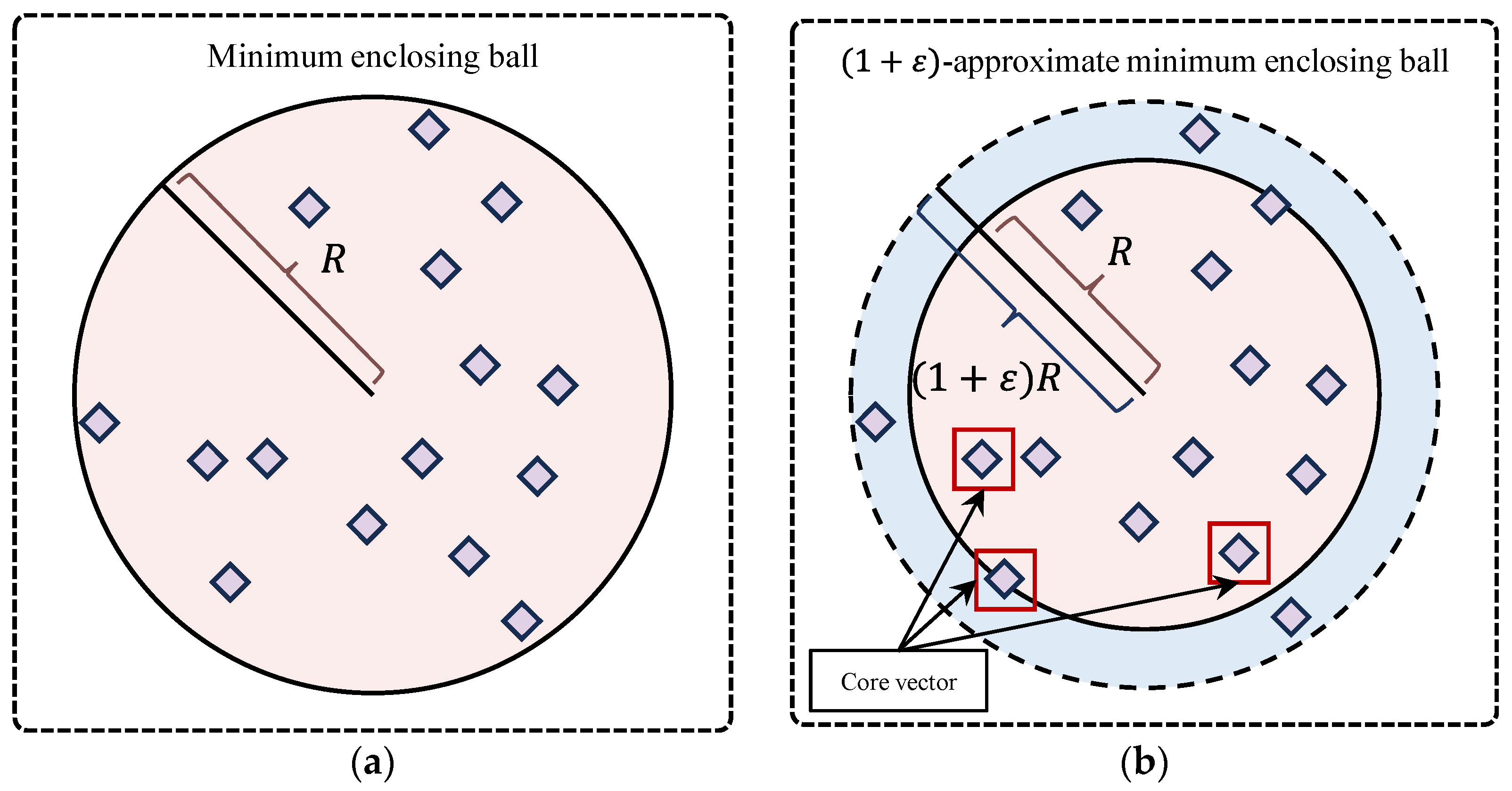
Figure 2 illustrates the core concept of the ( 1 + ε ) -approximation used in the core vector machine. The solid circle in both panel (a) and panel (b) represents the exact minimum enclosing ball with radius R . The dashed circle represents the ( 1 + ε ) -approximate minimum enclosing ball with radius ( 1 + ε ) R . The CVM technique iteratively expands the core set until all training points lie within the larger ball, guaranteeing an approximation factor of ( 1 + ε ) . This relaxation significantly reduces the number of required support vectors and accelerates the training process. The detailed iterative process will be consolidated into a generalized AUC maximization core vector machine algorithm and elaborated upon in the following subsection.

4.2. Generalized AUC Maximization Core Vector Machine Algorithm

According to the generalized AUC maximization learning objective constructed in the last subsection, we note that the key input is only the kernel matrix K . Most existing AUC maximization methods adopt the single fixed kernel to directly generate K , such as linear kernel or Gaussian kernel. In this work, we obtain a fused kernel matrix K ~ based on cross-diffusion in Equation (22). Therefore, by integrating K ~ into the dual problem Equations (40) and (41), we construct the complete generalized AUC maximization core vector machine (GAM-CVM) algorithm via multi-kernel learning. The following Algorithm 1 provides a detailed description of the pseudocode for GAM-CVM.
Algorithm 1: GAM-CVM
Input:  n +   positive   samples   x i + ,   n   negative   samples   x j ,   C 1 ,   C 2 ,   ε   and   n l o c
Output :   Core   vector   set   V S   and   Lagrange   multipliers   vector   α
1. 
For   all   ( n + + n )   samples ,   generate   the   sub - kernel   matrices   K ( 1 ) , K ( 2 ) , , K ( M ) ;
2. 
For   any   m = 1 , 2 , , M ,   calculate   the   natural   kernel   matrix   K ¯ ( m ) by calling Equation (18);
3. 
For   any   m = 1 , 2 , , M ,   calculate   the   local   kernel   matrix   L ¯ ( m ) by calling Equations (19) and (20);
4. 
While not converged do
For   any   m = 1 , 2 , , M ,   update   the   natural   kernel   matrix   K ¯ t ( m )   at   iteration   t   ( t = 1 , 2 , , T ) by calling Equation (21);
End while
Return   the   final   fused   kernel   matrix   K ~ by calling Equation (22);
5. 
Randomly   pick   a   sample   point   z i j = φ x i + φ x j   and   find   the   point   z u v   furthest   from   it .   Set   the   initial   core   set   V 0   as   z i j , z u v ,   the   initial   center   c 0 = 1 2 ( z i j + z u v )   and   the   initial   radius   as   R 0 = 1 2 z i j z u v = 1 2 φ x i + φ x j φ x u + + φ x v ;
6. 
While not converged do
For   iteration   s   ( t = 1 , 2 , , S ) ,   if   there   are   no   other   point   falls   outside   the   1 + ε - ball   ( c s 0 , 1 + ε R s ) , convergence;
Else ,   find   the   core   vector   z u v   that   is   furthest   away   from   the   center   c s ,   and   let   core   set   V s = V s z u v θ u v ;
End while
Return   the   core   set   V S ;
7. 
Calculate   the   optimal   α   based   on   the   core   set   V S by calling Equations (40) and (41).
It is worth noting that in steps 5 and 6 of Algorithm 1, the feature mapping φ · may be implicit, which prevents the center c s from being expressed in an explicit form. Nevertheless, for the purpose of identifying the farthest points, a direct approach can be employed using the technique described in [22]; the detailed distance computation is provided in Appendix A. Once the optimal α is obtained by solving the quadratic programming problems in Equations (40) and (41), the prediction of GAM-CVM for any sample x ˇ can be computed explicitly, as follows:
ω , φ ( x ˇ ) = i j α i j φ x i + φ x j φ x ˇ = i j α i j k x i + , x ˇ k x j , x ˇ .
Moreover, the ranking margin, which represents the bound of noise according to Section 2, can also be given as τ = α H + 1 C 1 E α / C 2 . Since GAM-CVM is fully built upon the CVM technique, it inherits the following advantages in the optimization stage when the fused affinity matrix is fixed in advance:
(1)
For a given approximation error ε , the size of the core set V s is bounded by O ( 1 / ε ) . Consequently, the maximum number of iterations required by Algorithm 1 is also O ( 1 / ε ) .
(2)
For a given ε , the asymptotic time complexity of Algorithm 1 is O ( n + n / ε 2 + 1 / ε 4 ) , which grows linearly with the number of sample pairs n + n . In contrast, conventional AUC maximization methods typically incur a quadratic time complexity of O ( ( n + n ) 2 ) [9].
(3)
For a given ε , the memory required to store all n = n + + n training sample pairs can be offloaded to external storage, so the naïve space complexity of O ( n + n ) is effectively ignored. Since only the core vectors are involved in solving Equation (40), the actual space complexity of Algorithm 1 is bounded by O ( 1 / ε 2 ) .
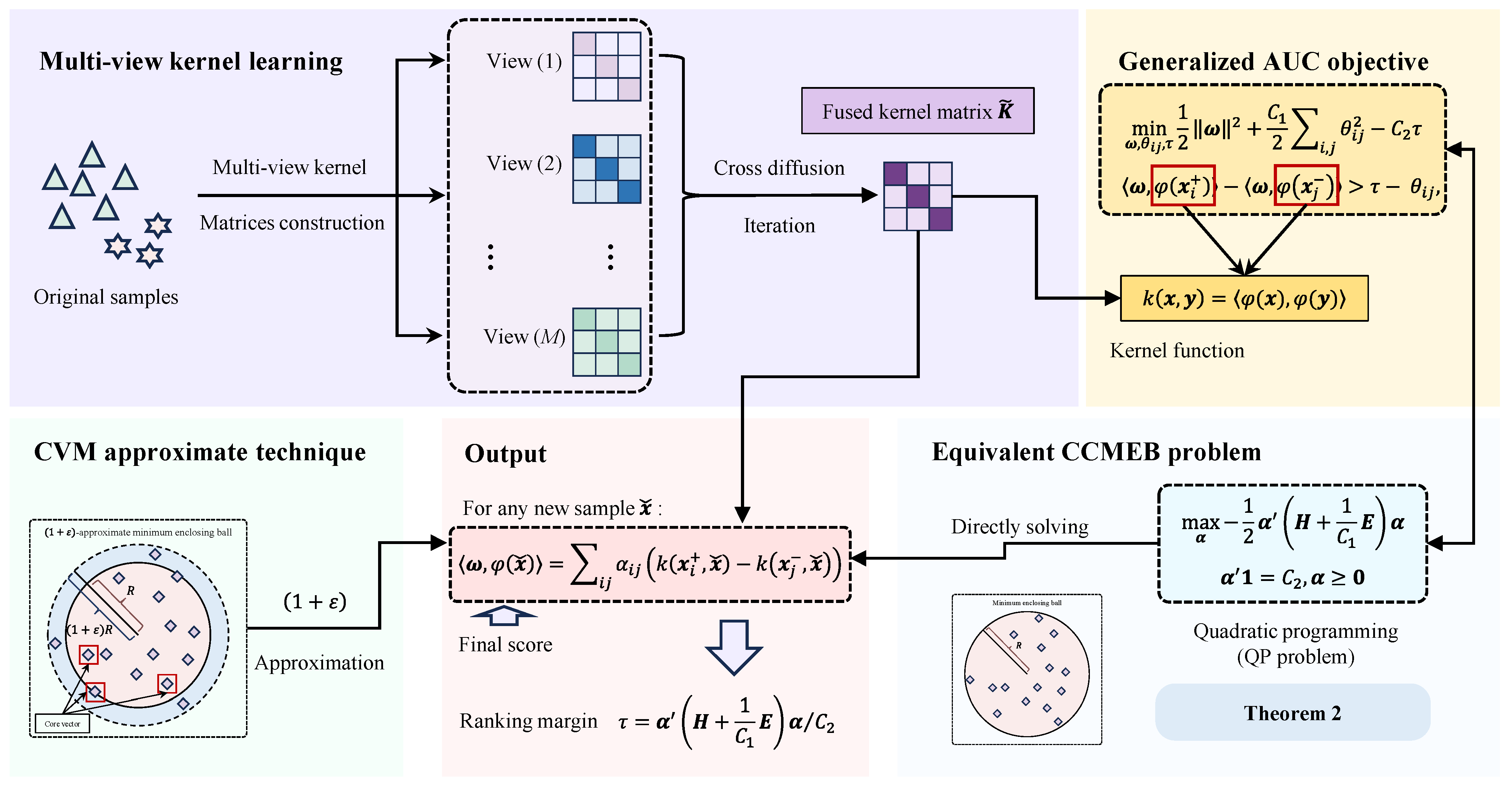
The above analysis follows the common practice in AUC maximization and kernel-based learning, where the computational complexity of the optimizer is typically characterized under a given kernel or affinity matrix, and the construction of the kernel or affinity matrix is treated as a separate preprocessing step. In summary, GAM-CVM inherits the theoretical convergence guarantees of core vector machines while benefiting from the rich representational power of multi-kernel fusion. This synergy enables fast and accurate AUC maximization on large-scale imbalanced data, as will be demonstrated in the experimental section. The complete workflow of the proposed GAM-CVM framework is illustrated in Figure 3.

5. Experimental Studies

In this section, we conduct five groups of experiments to comprehensively evaluate the proposed GAM-CVM framework. The first group evaluates the classification performance on 18 benchmark imbalanced datasets from the UCI repository, comparing GAM-CVM against representative AUC maximization methods, kernel-based methods, a tree-based ensemble method, and deep learning-based imbalanced classification methods. The second group provides statistical analysis using Friedman and post hoc tests to verify the significance of the observed performance differences. The third group investigates the sensitivity of the key hyperparameters, including the regularization coefficients C 1 , C 2 and the approximation error ε . The fourth group presents an ablation study to quantify the contribution of each sub-kernel. The fifth group demonstrates the practical applicability of GAM-CVM on a real-world Alzheimer’s disease classification task.
For the first two groups, we compare GAM-CVM with eight competing methods: the standard AUC maximizing support vector machine (AUCSVM) [9], large-scale nonlinear AUC maximization via triply stochastic gradients (TSAM) [14], the AUC-based extreme learning machine (AUC-ELM) [15], the adversarial de-overlapping learning machine (De-OVL) [16], the fast AUC maximization learning machine ( ρ -AUCCVM) [17], a gradient boosting decision tree-based ensemble method (GBDT) [30], and two recent deep learning-based imbalanced classification methods, i.e., a convolutional neural network with class weights and early-stopping techniques, denoted as CE-CNNs, and the cluster-guided contrastive imbalanced classification network (C3GNN) [31,32].
For fairness, all the competing methods are implemented under their recommended parameter settings. For the proposed GAM-CVM, the three hyperparameters are tuned via grid search: C 1 { 0.001 , 0.01 , 0.1 , 0.5 , 1 , 5 , 10 , 100 } , C 2 { 0.001 , 0.01 , 0.1 , 0.5 , 1 , 5 , 10 , 100 } and ε { 10 8 , 10 7 , 10 6 , 10 5 , 10 4 , 0.001 , 0.01 , 0.1 } . For multi-kernel construction, as stated in Section 3, the Gaussian kernel bandwidth is set as the median standard deviation of all samples, and the local neighborhood size n l o c is searched in { 4 , 8 , 16 , 32 , 64 , 128 } .
All experiments are implemented in MATLAB R2023b on a workstation with an Intel (R) Core (TM) i7-14700KF @ 3.40 GHz and 32 GB of RAM.

5.1. Evaluation on UCI Datasets

To comprehensively assess the performance of the proposed GAM-CVM, we conduct experiments on 18 benchmark datasets selected from the UCI Machine Learning Repository (https://archive.ics.uci.edu/). These datasets were selected to provide a diverse and reproducible benchmark for imbalanced binary classification. Specifically, all datasets are publicly available, can be formulated as clear positive–negative classification tasks required by pairwise AUC maximization, and have been widely used in imbalanced learning studies. They cover different application domains, including medical diagnosis, biological analysis, document/image recognition, industrial monitoring, and financial risk assessment. They also vary substantially in class imbalance, feature dimensionality, and pairwise sample scale. As summarized in Table 1, the imbalance ratios range from 1.14 to 194.46. The number of features ranges from 3 to 72, and the number of positive–negative sample pairs ranges from 5365 to 14,733,244. Since AUC-based learning is performed on positive–negative sample pairs, Table 1 reports the number of sample pairs n + n , the number of positive samples n + , the number of negative samples n , the number of features, and the imbalance ratio for each dataset.
Since the proposed method is designed as a generalized AUC maximization framework, AUC is adopted as the primary metric for evaluating pairwise ranking performance. This choice is consistent with the learning objective of GAM-CVM and with the compared AUC maximization baselines. In addition, we report the Average Precision (AP) to provide a threshold-independent precision-recall-oriented evaluation for assessing minority-class ranking performance [33]. For each dataset, we perform 10-fold stratified cross-validation, ensuring that the class proportion is preserved in each fold. The reported results on each dataset are averaged over the 10 folds for 20 runs. All competing methods are implemented with their recommended hyperparameter settings as described in Section 5. For GAM-CVM, the parameters are tuned via grid search on the training set of each fold.
Table 2 reports the mean AUC and AP values achieved by GAM-CVM and the eight competing methods on the 18 datasets. The best performance for each dataset is highlighted in bold. Several observations can be drawn from the results. First, GAM-CVM achieves the best overall performance and obtains the highest AUC and AP on most datasets, demonstrating the effectiveness of integrating generalized AUC maximization, multi-kernel fusion, and core vector machine optimization. On highly imbalanced datasets such as Abalone-19, Mammography, Ozone_level, and PageBlocks-II, GAM-CVM remains highly competitive and often achieves the best or second-best performance, indicating its robustness under severe class skewness. Second, among the AUC-based competing methods, ρ -AUCCVM and TSAM generally perform better than early AUC-based approaches such as AUCSVM and AUC-ELM, confirming the benefits of margin-based ranking optimization and stochastic approximation. However, their reliance on a single fixed kernel may limit their ability to capture complex data structures, especially on datasets with heterogeneous feature distributions such as Spambase, Ionosphere, and Ozone_level. Third, the newly added GBDT baseline shows strong competitiveness on several datasets, especially in terms of AP on Ozone_level and Pima, confirming the importance of including tree-based ensemble methods in imbalanced tabular classification. Nevertheless, GAM-CVM still achieves a better average rank across all datasets and metrics. This suggests that GAM-CVM and GBDT have complementary strengths: GBDT is highly competitive for general tabular classification, while GAM-CVM is specifically designed for ranking-oriented AUC optimization with multi-kernel similarity modeling. Fourth, the deep learning methods CE-CNNs and C3GNN show competitive performance on some larger datasets, but their performance is less stable across small or highly skewed datasets. In contrast, GAM-CVM maintains robust overall performance across varying dataset sizes and imbalance ratios, owing to its multi-kernel representation and core set approximation.
In addition to classification accuracy, we evaluate the optimization efficiency of all compared methods. Table 3 reports the average running time of the classifier optimization stage on the 18 UCI datasets. For GAM-CVM, the reported time corresponds to the CCMEB/CVM-based generalized AUC optimization stage under a given fused affinity matrix, while the independent multi-kernel affinity construction and cross-diffusion fusion stage is not included. Several observations can be made from the results. First, GAM-CVM consistently achieves the lowest optimization-stage running time on all datasets, owing to its core vector machine formulation that reduces the effective number of pairwise constraints from n + n to a much smaller core set. Even on the largest dataset, Letter-z, GAM-CVM completes training in approximately 16.35 s, which is about 88.5% faster than AUCSVM. Second, AUCSVM and the two deep learning methods, CE-CNNs and C3GNN, generally require the largest training times. AUCSVM suffers from exhaustive pairwise quadratic programming, while the deep learning methods require iterative backpropagation and substantial parameter tuning. The newly added GBDT baseline also incurs non-negligible computational cost on several datasets, especially Mammography and PageBlocks-II. Third, among the remaining AUC-based methods, ρ -AUCCVM is the fastest approach because it shares a similar core set approximation strategy with GAM-CVM, followed by De-OVL and TSAM, whereas AUC-ELM exhibits moderate training times. The clear advantage of GAM-CVM in training efficiency, combined with its strong classification performance demonstrated in Table 2, underscores the practical value of integrating multi-kernel fusion with core vector machine optimization for large-scale imbalanced classification tasks.
Overall, the experimental results on the 18 UCI datasets confirm that GAM-CVM achieves the best overall ranking among all compared methods in terms of AUC and AP, while maintaining the lowest optimization-stage training time across all datasets. Its advantage is particularly evident on highly imbalanced datasets such as Abalone-19, Mammography, Ozone_level, and PageBlocks-II, as well as on high-dimensional datasets such as Ionosphere, Ozone_level, Sonar, and Spambase. These results validate the effectiveness of the proposed multi-kernel fusion strategy and core vector machine optimization.

5.2. Statistical Analysis

To assess whether the observed performance differences among the compared methods are statistically significant, we conduct a comprehensive statistical analysis. Specifically, we employ the Friedman test as a non-parametric alternative to repeated-measures analysis of variance (ANOVA) [19], which ranks the algorithms independently on each dataset and evaluates the null hypothesis that all methods perform equivalently. Subsequently, a post hoc Nemenyi test is performed to identify pairwise differences between GAM-CVM and the competing methods when the null hypothesis is rejected [34].
The Friedman test ranks each method on each dataset according to its performance metric. In our analysis, we use the average rankings across both AUC and AP for all 18 datasets, resulting in a total of 36 ranking observations (18 datasets × 2 metrics). Table 4 reports the average rankings of the nine methods, and the proposed GAM-CVM achieves the best average rank of 1.2500. Under the Friedman test with nine methods and 36 observations, the Friedman statistic follows an F-distribution with 8 and 280 degrees of freedom, where nine is the number of methods and 36 is the number of ranking observations. The computed FF statistic is 120.1123, which substantially exceeds the critical value of 1.9715 at the 0.05 significance level. Consequently, the null hypothesis that all methods perform equally is rejected, confirming that significant differences exist among the compared algorithms.
Having rejected the null hypothesis, we proceed with the Nemenyi post hoc test to determine which specific pairs of methods differ significantly. The critical difference (CD) is calculated as 2.0025. Two methods are considered significantly different if the difference between their average rankings exceeds this CD value. Table 5 presents the results of the post hoc test comparing the best-performing GAM-CVM against each of the other eight methods. It should be noted that the difference between GAM-CVM and GBDT is not statistically significant at the 0.05 level. Therefore, the results should not be interpreted as showing that GAM-CVM universally dominates GBDT. Rather, GAM-CVM is preferable in scenarios where ranking-oriented optimization, kernel-based similarity modeling and efficient pairwise AUC learning are required. GBDT remains a strong and practical baseline for general tabular classification, whereas GAM-CVM provides a principled alternative when the goal is to directly optimize positive–negative ranking relationships under class imbalance. In contrast, the differences between GAM-CVM and the remaining seven methods range from 2.5556 to 7.2222, all exceeding the CD value. Thus, the null hypothesis of equal performance is rejected for these seven comparisons, confirming that GAM-CVM significantly outperforms most of the compared imbalanced classification methods.
These statistical results provide strong evidence that GAM-CVM achieves superior overall performance compared to the majority of the compared imbalanced classification methods. Although the difference between GAM-CVM and GBDT does not reach statistical significance, GAM-CVM obtains the best average rank and consistently exhibits the lowest optimization-stage training time, as demonstrated in Table 3. The significant advantages over the other seven methods further validate the effectiveness of integrating multi-kernel fusion with core vector machine optimization for imbalanced classification tasks.

5.3. Parameter Sensitivity Analysis

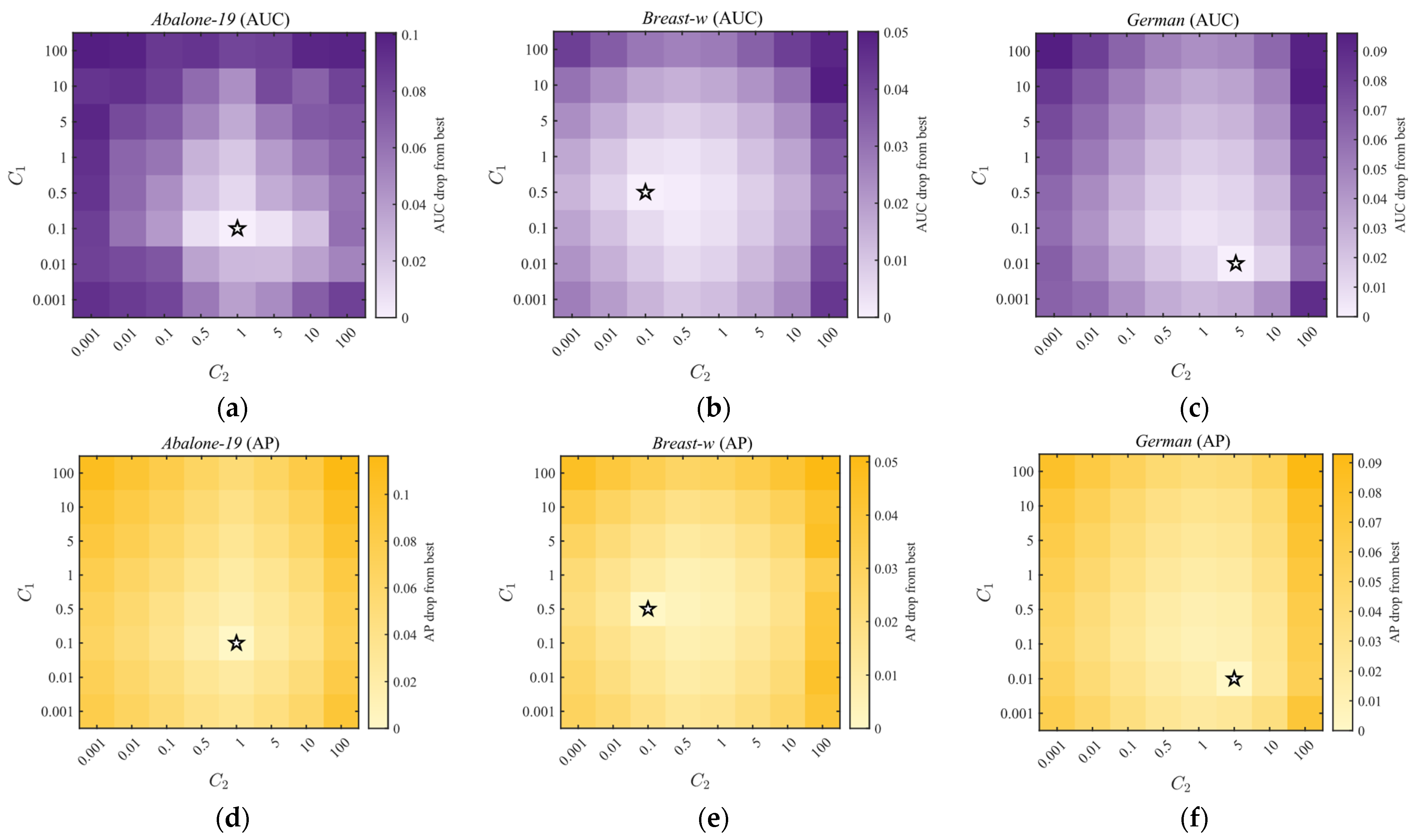
To investigate the influence of the key hyperparameters on the proposed GAM-CVM, we conduct a parameter sensitivity analysis for the two regularization coefficients C 1 and C 2 , as well as the approximation error ε . Specifically, C 1 and C 2 are searched within 0.001 0.01 0.1 0.5 1 5 10 100 and ε is 10 8 10 7 10 6 10 5 10 4 0.001 0.01 0.1 . Figure 4 presents the joint sensitivity of C 1 and C 2 on three representative datasets, including Abalone-19, Breast-w, and German, where each heatmap visualizes the performance drop from the best result under different parameter combinations. The first three heatmaps report AUC, while the last three heatmaps report AP. The heatmaps for the remaining 15 datasets are provided in Appendix B.
As shown in Figure 4, the optimal combination of C 1 and C 2 varies across datasets, indicating that the balance between the ranking loss and the regularization term is data-dependent. For Abalone-19, the best performance is achieved at C 1 = 0.1 and C 2 = 1 , where GAM-CVM obtains an AUC of 0.8216 and an AP of 0.5365. For Breast-w, the optimal region shifts to C 1 = 0.5 and C 2 = 0.1 , corresponding to an AUC of 0.9921 and an AP of 0.9747. For German, the best performance appears at C 1 = 0.01 and C 2 = 5 , where the AUC and AP reach 0.7540 and 0.7638, respectively. These results suggest that no single parameter pair is uniformly optimal for all datasets.
Nevertheless, the heatmaps also reveal that GAM-CVM is not overly sensitive to small perturbations around the optimal parameter regions. In most cases, a relatively stable plateau can be observed around the best parameter combination, where both AUC and AP remain close to their peak values. However, when C 1 or C 2 deviates from the suitable range by several orders of magnitude, the performance decreases noticeably, especially on more challenging datasets. This confirms the necessity of parameter tuning, while also showing that the proposed method has a reasonably stable operating region.
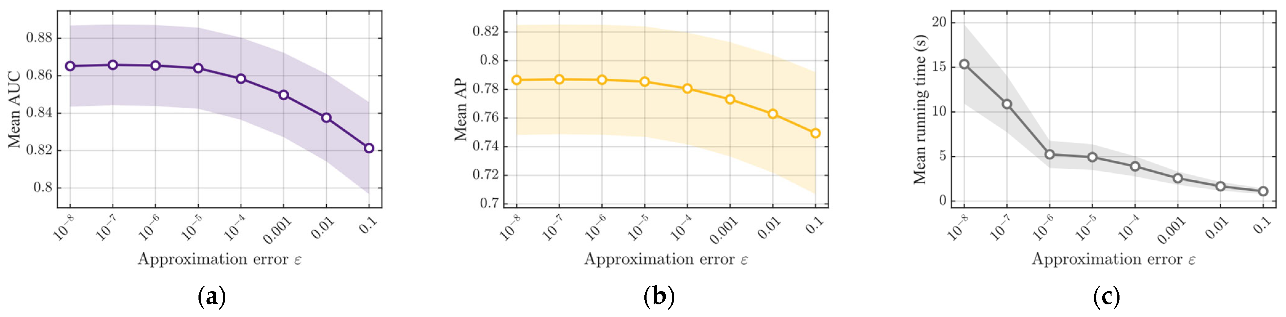
Figure 5 further reports the sensitivity of GAM-CVM with respect to the approximation error ε , where the three curves show the average AUC (Figure 5a), average AP (Figure 5b), and average optimization-stage running time over all 18 datasets (Figure 5c), and the shaded bands indicate the variation across datasets. In general, smaller ε values lead to slightly higher AUC and AP because a smaller approximation error allows the CVM procedure to preserve a larger and more accurate core set. However, the performance improvement becomes marginal when ε is sufficiently small. For example, when ε changes from 10 8 to 10 5 , the average AUC and AP remain almost unchanged, indicating that further reducing ε   provides limited additional accuracy gain.
By contrast, the optimization-stage running time is much more sensitive to ε . As shown in Figure 5c, the average running time decreases rapidly as ε   increases. The average optimization-stage running time decreases from 15.37 s at ε = 10 8 to 10.89 s at ε = 10 7 , 5.24 s at ε = 10 6 , and 3.90 s at ε = 10 4 . When ε   is further increased to 10 1 , the running time decreases to only 1.10 s. This confirms that a larger approximation error can substantially reduce the computational burden by retaining fewer core vectors during the optimization process.
Overall, the parameter sensitivity analysis demonstrates that GAM-CVM benefits from appropriate tuning of C 1 , C 2 , and ε , but its performance remains stable within a reasonable neighborhood of the optimal values. The heatmap-based visualization provides a clear interpretation of the parameter effects, making the robustness and efficiency trade-off of the proposed method easier to observe.

5.4. Ablation Study for Multi-Kernel Learning

As stated in Section 3, this study mainly employs three representative sub-kernels for experimental validation. To investigate the contribution of each sub-kernel in the proposed multi-kernel fusion, we conducted an ablation study on the 18 UCI benchmark datasets. Table 6 reports the average AUC and AP achieved by GAM-CVM under different sub-kernel combinations, where K1, K2 and K3 denote the Gaussian kernel, the Pearson correlation coefficient-based kernel, and the density-based kernel, respectively. The full combination of all three sub-kernels is the proposed GAM-CVM, whose results are consistent with those in Table 2.
As shown in Table 6, the full model (K1 + K2 + K3) achieves the highest AUC on every dataset and the highest AP on 17 out of 18 datasets. The only exception is the AP on Ionosphere, where the combination of K1 and K2 slightly outperforms the full model. This indicates that for this particular dataset and metric, adding the density-based kernel may introduce a small amount of redundancy or overfitting, while the complementary information from K1 and K2 is already sufficient to capture the essential ranking structure. Nevertheless, the difference is marginal, and the full model remains highly competitive.
When only a single sub-kernel is used, the best performance is dataset-dependent. For example, on Glass-6, the density-based kernel alone yields an AUC of 0.8742, notably higher than the other two single sub-kernels, indicating that local density information is particularly effective for this dataset. Conversely, on Ionosphere, the Gaussian kernel achieves the highest single sub-kernel AUC, while on Letter-z, the Pearson correlation kernel obtains the best single sub-kernel AP. This diversity demonstrates that each sub-kernel captures complementary aspects of the data structure, and their relative importance varies across datasets. Combining two sub-kernels generally improves over any single sub-kernel, but the improvement is not uniform. For instance, on Abalone-19, K2 + K3 yields an AUC of 0.8021, which is substantially higher than the best single sub-kernel, while adding K1 further boosts the performance to 0.8216. On the other hand, for Breast-w, the gain from using two sub-kernels over the best single sub-kernel is marginal, reflecting that the dataset is already well separated, even with a single kernel. Moreover, the relative ordering of two-sub-kernel combinations is not always consistent: on Glass-6, K1 + K3 slightly outperforms K1 + K2, whereas on Sonar, the opposite holds. Such realistic fluctuations confirm that the interaction between sub-kernels is not simply additive and that a systematic fusion is necessary.
In summary, the ablation study validates that each of the three sub-kernels captures unique and complementary information. The multi-kernel fusion strategy in GAM-CVM successfully integrates these complementary similarity representations, leading to consistently strong performance across almost all datasets and metrics.

5.5. Application in Alzheimer’s Disease MRI Brain Scan Classification

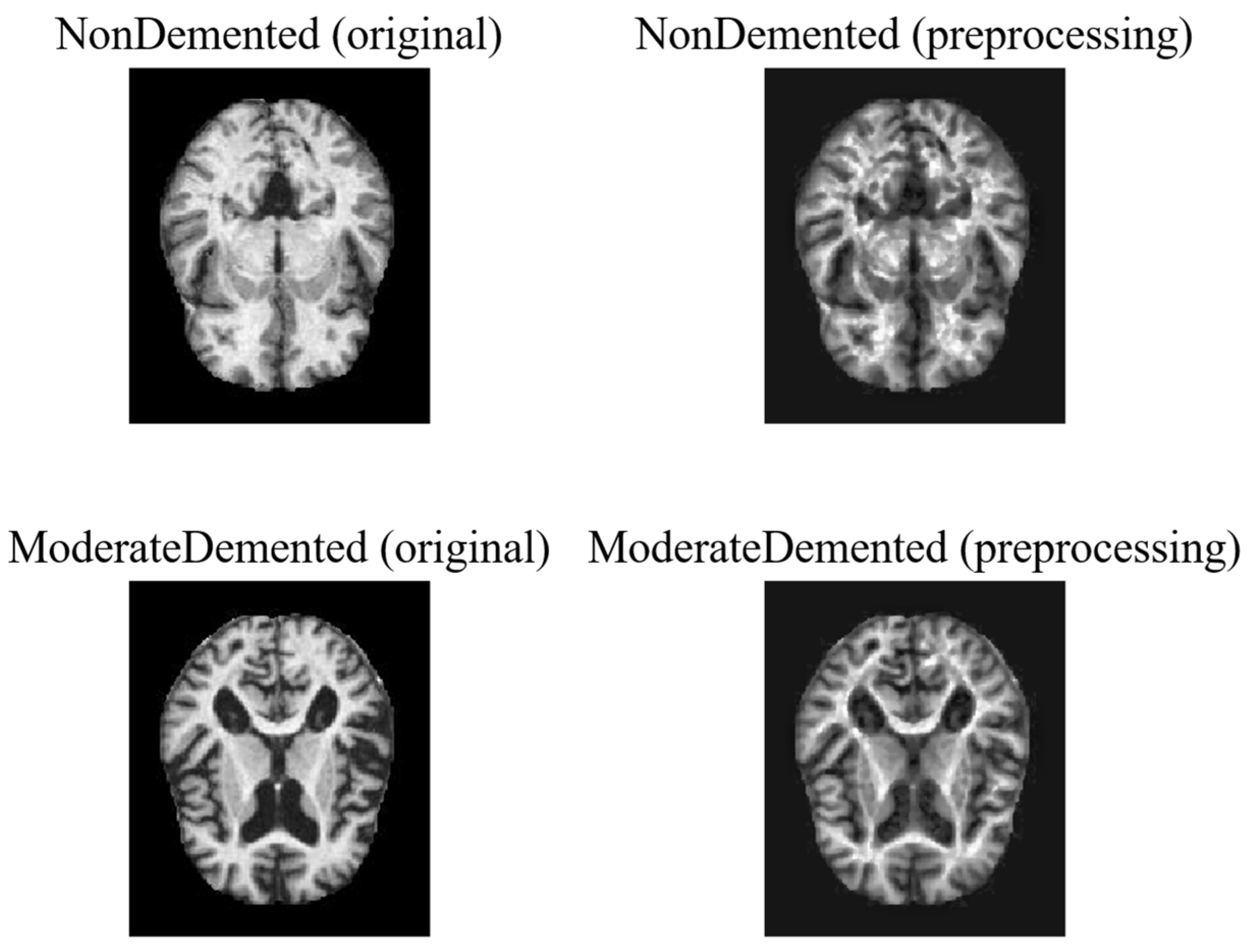
To further evaluate the practical applicability of the proposed GAM-CVM framework in real-world medical diagnosis, we conduct an experiment on the public Alzheimer’s Disease Detection Dataset [35]. This dataset consists of 6400 axial T1-weighted MRI brain scans in JPG format ( 208 × 176 pixels), originally classified into four progressive stages: NonDemented, VeryMildDemented, MildDemented, and ModerateDemented. Since the objective of this study is imbalanced binary classification, we extract only the two extreme classes: NonDemented (healthy) and ModerateDemented (severe Alzheimer’s disease). The resulting subset exhibits a severe class imbalance, as summarized in Table 7. All images undergo standard preprocessing: grayscale conversion, median filtering (3 × 3) for denoising, and contrast-limited adaptive histogram equalization (CLAHE) to enhance local contrast [36,37]. Finally, pixel intensities are normalized to the range [0, 1]. Figure 6 illustrates the effect of this preprocessing pipeline on one representative image from each class. The enhanced images clearly reveal cortical atrophy and ventricular enlargement in the ModerateDemented case compared to the healthy control.
After preprocessing, we extract a histogram of oriented gradient (HOG) features from each image, which have been proven effective for capturing shape and texture information in brain MRI [38]. The HOG descriptor is computed with a cell size of 8   ×   8 pixels, a block size of 2   ×   2 cells, and 9 orientation bins, yielding a feature vector of 17,884 dimensions. To reduce computational cost while preserving 95% variance, principal component analysis is applied to project the features into a 200-dimensional subspace. The resulting feature matrix serves as input to all compared classifiers. We compare GAM-CVM against the same eight competing methods as in Section 5.1. All hyperparameters are tuned via grid search on the training set of each fold, using the ranges specified in the first three paragraphs of Section 5. For the deep learning baselines (CE-CNNs and C3GNN), we adopt their recommended architectures and apply data augmentation to the positive class (ModerateDemented) to mitigate overfitting. Ten-fold stratified cross-validation is performed on the training set, and the average AUC and AP on the test set over 20 runs are reported in Table 8.
As reported in Table 8, GAM-CVM achieves the highest AUC and AP among all competing methods on the test set. Compared with the second-best method in terms of each metric, GAM-CVM achieves an absolute improvement of 1.42 percentage points in AUC over ρ -AUCCVM and 1.64 percentage points in AP over GBDT. The AP improvement is particularly meaningful for the extremely rare ModerateDemented class, since AP provides a precision-recall-oriented evaluation of minority-class identification under severe class imbalance. The multi-kernel fusion strategy of GAM-CVM effectively integrates complementary similarity measures, which helps capture subtle pathological patterns that may not be well represented by a single kernel. Moreover, the core vector machine formulation reduces the effective number of pairwise constraints, allowing the model to handle the imbalanced pairwise learning problem efficiently. These results confirm that GAM-CVM is a robust and practical tool for computer-aided diagnosis of Alzheimer’s disease under severe class imbalance.


6. Conclusions

In this paper, we propose GAM-CVM, a fast imbalanced classification framework that integrates multi-kernel learning with core vector machine optimization. By fusing complementary sub-kernels through cross-diffusion and introducing a flexible ranking margin into the generalized AUC objective, GAM-CVM improves similarity representation and robustness to noise. Given the fused affinity matrix, the CCMEB reformulation reduces the effective pairwise optimization burden and improves the optimization-stage efficiency of GAM-CVM, while the affinity construction and cross-diffusion fusion are handled as an independent preprocessing module. Experiments on 18 UCI datasets and a real-world Alzheimer’s disease MRI classification task show that GAM-CVM achieves the best overall average ranking among nine compared methods in terms of AUC and AP while maintaining the lowest optimization-stage running time. The Friedman and Nemenyi tests further confirm that GAM-CVM significantly outperforms most competing methods.
Several directions remain for future work. First, although AUC and AP provide complementary ranking-oriented evaluations, the current optimization objective is still built on generalized AUC maximization. Extending the center-constrained minimum enclosing ball framework to directly optimize precision-recall-oriented objectives is therefore a meaningful direction. Second, although the current benchmark covers diverse imbalance ratios, feature dimensions, and sample-pair scales, further evaluation on larger benchmark suites such as KEEL and OpenML will help validate the robustness of GAM-CVM across broader imbalanced learning scenarios. Third, the multi-kernel construction and cross-diffusion fusion stage can still be costly for massive datasets; thus, scalable approximations such as Nyström approximation, random Fourier features, and anchor-based graph construction will be explored. Finally, extending GAM-CVM to multi-class, multi-label, and deep representation learning settings may further broaden its applicability to complex real-world tasks such as medical image analysis and text classification.

Author Contributions

Conceptualization, Y.S. and M.W.; methodology, Y.S. and S.W.; software, Y.S. and E.Z.; validation, Y.S., E.Z. and K.Z.; formal analysis, M.W.; investigation, Y.S.; resources, S.W.; data curation, Y.S.; writing—original draft preparation, Y.S. and E.Z.; writing—review and editing, M.W. and K.Z.; visualization, M.W.; supervision, K.Z.; project administration, Y.S.; funding acquisition, Y.S., S.W. and K.Z. All authors have read and agreed to the published version of the manuscript.

Funding

This work was supported in part by the National Key R&D Project under Grant 2022YFE0112400, in part by the Natural Science Foundation of Jiangsu Province (Basic Research Special Fund) under Grant BK20251751, in part by the Natural Science Key Research Projects of Jiangsu Education Department under Grant 22KJA520009 and the Research Project of Jiangsu Vocational College of Information Technology under Grant JSITKY202511.

Data Availability Statement

The datasets and source code are available at the following repository: https://gitee.com/JNUsyc/gam-cvm.git (accessed on 15 May 2026).

Conflicts of Interest

The authors declare no conflicts of interest.

Appendix A

Please note that, for steps 5 and 6 of Algorithm 1, the mapping φ · may be implicit, hence the center c s also cannot be calculated in an explicit form. Actually, when the goal is to locate the farthest points, we can directly determine them via the following approach. That is, instead of directly computing the center c s , we can evaluate the distance between the candidate point z i j = φ x i + φ x j and c s . Specifically, the distance can be calculated by
c ( φ x i + φ ( x j ) ) 2 + δ i 2 = c 2 + φ ( x i + ) φ ( x j ) 2 2 c ( φ ( x i + ) φ ( x j ) ) + δ i 2 .
Then we introduce the Lagrange multipliers, the distance can be expressed by
i j u v α i j α u v φ x i + φ x u + φ x i + φ x v φ x j φ x u + + φ x j φ x v + φ x i + φ x i + + φ x j φ x j 2 φ x i + φ x j 2 u v α u v ( φ x u + φ x v φ x i + u v α u v ( φ x u + φ x v φ x j ) + δ i 2 .
Furthermore, it can be written as
i j u v α i j α u v k x i + , x u + k x i + , x v k x j , x u + + k x j , x v + k x i + , x i + + k x j , x j 2 k x i + , x j 2 u v α u v k x i + , x u + + 2 u v α u v k x i + , x v + 2 u v α u v k x j , x u + 2 u v α u v k x j , x v + δ i 2 .
As each term in Equation (A3) is represented by the kernel function, we can compute the distance without the need to explicitly obtain the ball’s center.

Appendix B

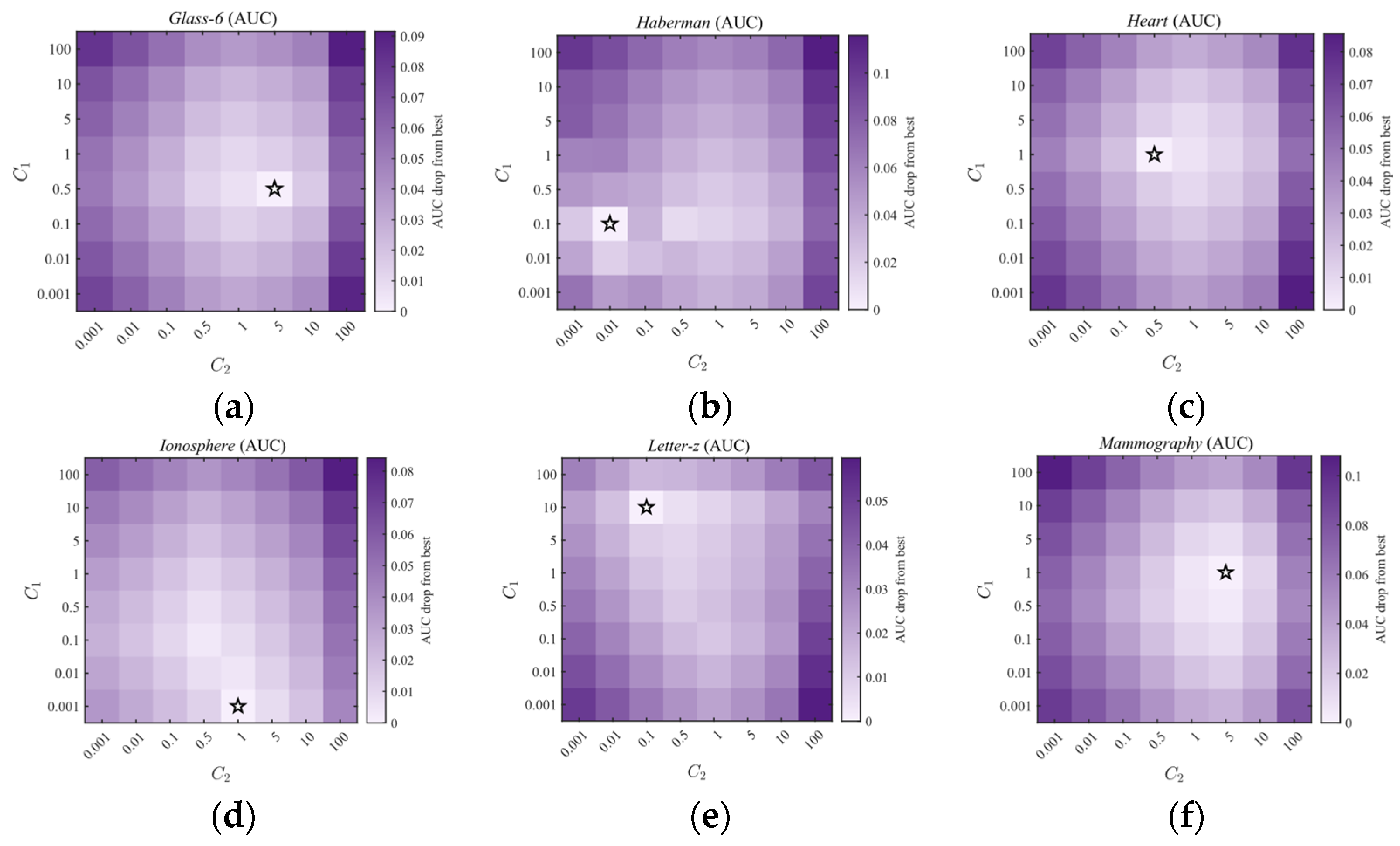
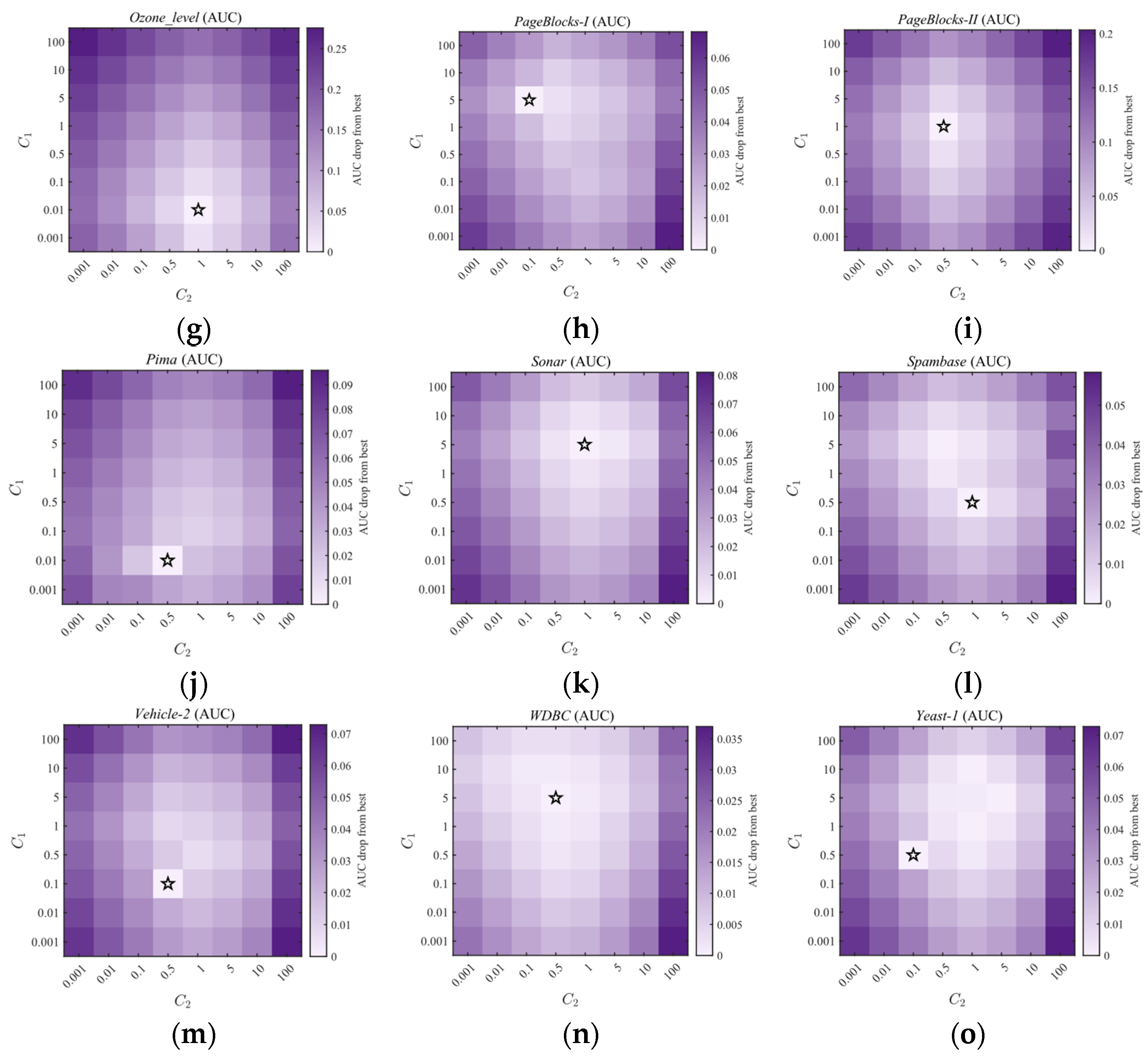
Figure A1. Joint sensitivity analysis of the regularization coefficients based on AUC performance drop on the remaining 15 UCI datasets. (a) Glass-6; (b) Haberman; (c) Heart; (d) Ionosphere; (e) Letter-z; (f) Mammography; (g) Ozone_level; (h) PageBlocks-I; (i) PageBlocks-II; (j) Pima; (k) Sonar; (l) Spambase; (m) Vehicle-2; (n) WDBC; (o) Yeast-1.
Electronics 15 02228 g0a1aElectronics 15 02228 g0a1b
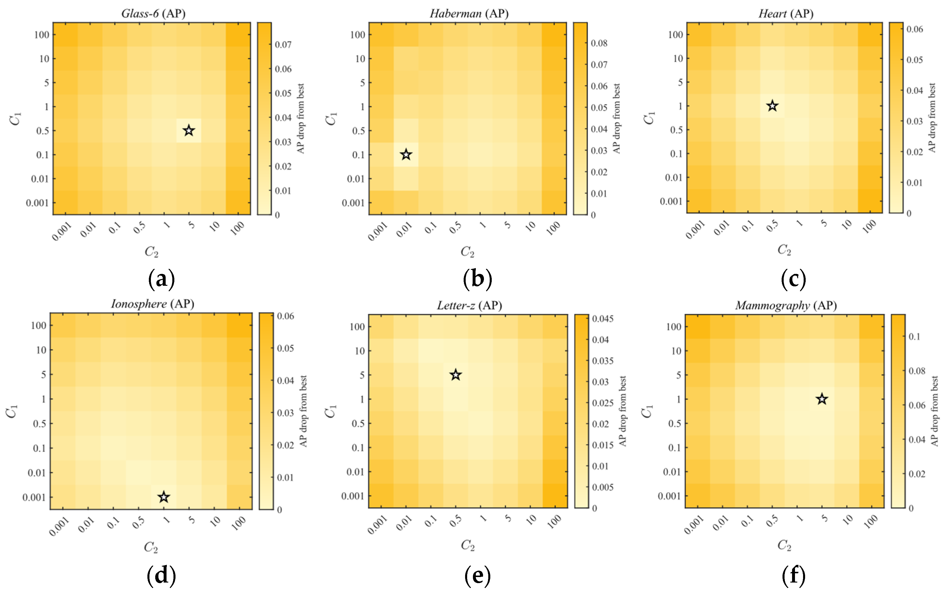
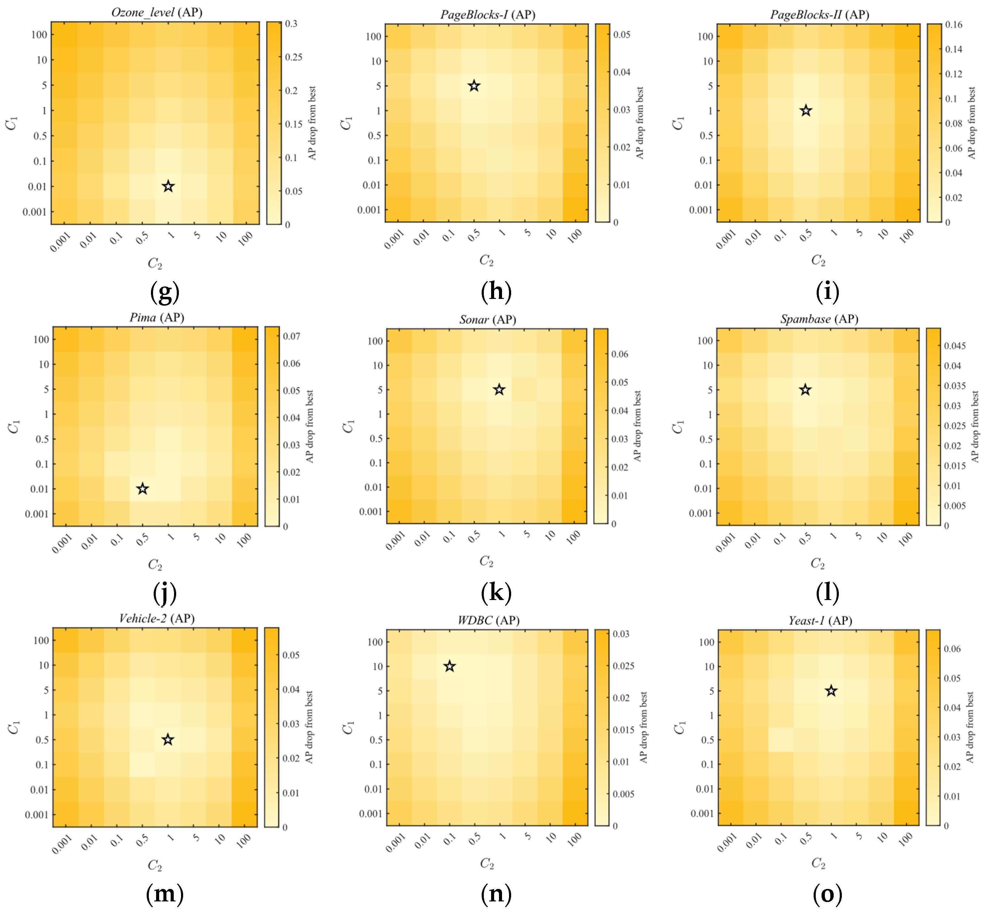
Figure A2. Joint sensitivity analysis of the regularization coefficients based on AP performance drop on the remaining 15 UCI datasets. (a) Glass-6; (b) Haberman; (c) Heart; (d) Ionosphere; (e) Letter-z; (f) Mammography; (g) Ozone_level; (h) PageBlocks-I; (i) PageBlocks-II; (j) Pima; (k) Sonar; (l) Spambase; (m) Vehicle-2; (n) WDBC; (o) Yeast-1.
Electronics 15 02228 g0a2aElectronics 15 02228 g0a2b

References

  1. Qtaish, A.; Albashish, D.; Braik, M.; Alshammari, M.T.; Alreshidi, A.; Alreshidi, E.J. Memory-Based Sand Cat Swarm Optimization for Feature Selection in Medical Diagnosis. Electronics 2023, 12, 2042. [Google Scholar] [CrossRef]
  2. Nti, I.K.; Quarcoo, J.A.; Aning, J.; Fosu, G.K. A mini-review of machine learning in big data analytics: Applications, challenges, and prospects. Big Data Min. Anal. 2022, 5, 81–97. [Google Scholar] [CrossRef]
  3. Bej, S.; Davtyan, N.; Wolfien, M.; Nassar, M.; Wolkenhauer, O. LoRAS: An oversampling approach for imbalanced datasets. Mach. Learn. 2021, 110, 279–301. [Google Scholar] [CrossRef]
  4. Seol, D.H.; Choi, J.E.; Kim, C.Y.; Hong, S.J. Alleviating Class-Imbalance Data of Semiconductor Equipment Anomaly Detection Study. Electronics 2023, 12, 585. [Google Scholar] [CrossRef]
  5. Araf, I.; Idri, A.; Chairi, I. Cost-sensitive learning for imbalanced medical data: A review. Artif. Intell. Rev. 2024, 57, 80. [Google Scholar] [CrossRef]
  6. Chen, Z.; Duan, J.; Kang, L.; Qiu, G. Class-imbalanced deep learning via a class-balanced ensemble. IEEE Trans. Neural Netw. Learn. Syst. 2021, 33, 5626–5640. [Google Scholar] [CrossRef]
  7. Cho, H.; Sung, J.-H.; Kang, H.-J.; Jang, J.; Shin, D. Quantifying Cyber Resilience: A Framework Based on Availability Metrics and AUC-Based Normalization. Electronics 2025, 14, 2465. [Google Scholar] [CrossRef]
  8. Wang, S.; Yao, X. Using class imbalance learning for software defect prediction. IEEE Trans. Reliab. 2013, 62, 434–443. [Google Scholar] [CrossRef]
  9. Brefeld, U.; Scheffer, T. AUC maximizing support vector learning. In Proceedings of the ICML 2005 Workshop on ROC Analysis in Machine Learning, Bonn, Germany, 11 August 2005. [Google Scholar]
  10. Zhou, B.; Ying, Y.; Skiena, S. Online AUC Optimization for Sparse High-Dimensional Dataset. In Proceedings of the 2020 IEEE International Conference on Data Mining (ICDM), Sorrento, Italy, 17–20 November 2020. [Google Scholar] [CrossRef]
  11. Ding, Y.; Zhao, P.; Hoi, S.; Ong, Y.S. An adaptive gradient method for online AUC maximization. In Proceedings of the AAAI Conference on Artificial Intelligence, Austin, TX, USA, 25–30 January 2015. [Google Scholar] [CrossRef]
  12. Lei, Y.; Ying, Y. Stochastic proximal AUC maximization. J. Mach. Learn. Res. 2021, 22, 1–45. [Google Scholar]
  13. Liu, M.; Zhang, X.; Chen, Z.; Wang, X.; Yang, T. Fast stochastic AUC maximization with O (1/n)-convergence rate. In Proceedings of the International Conference on Machine Learning, Stockholm, Sweden, 10–15 July 2018. [Google Scholar]
  14. Dang, Z.; Li, X.; Gu, B.; Deng, C.; Huang, H. Large-scale nonlinear AUC maximization via triply stochastic gradients. IEEE Trans. Pattern Anal. Mach. Intell. 2020, 44, 1385–1398. [Google Scholar] [CrossRef] [PubMed]
  15. Wang, G.; Wong, K.W.; Lu, J. AUC-Based Extreme Learning Machines for Supervised and Semi-Supervised Imbalanced Classification. IEEE Trans. Syst. Man Cybern. Syst. 2021, 51, 7919–7930. [Google Scholar] [CrossRef]
  16. Sun, Y.; Vong, C.M.; Wang, S. Adversarial de-overlapping learning machines for supervised and semi-supervised learning. Int. J. Mach. Learn. Cybern. 2025, 16, 2249–2267. [Google Scholar] [CrossRef]
  17. Sun, Y.; Vong, C.M.; Wang, S. Fast AUC Maximization Learning Machine With Simultaneous Outlier Detection. IEEE Trans. Cybern. 2023, 53, 6843–6857. [Google Scholar] [CrossRef]
  18. Liu, J.; Liu, X.; Yang, Y.; Liao, Q.; Xia, Y. Contrastive multi-view kernel learning. IEEE Trans. Pattern Anal. Mach. Intell. 2023, 45, 9552–9566. [Google Scholar] [CrossRef]
  19. Sun, Y.; Sun, Q.; Zhou, E.; Wu, M.; Wang, S. Enhanced label propagation via triply affinity fusion for semi-supervised classification. J. Supercomput. 2025, 81, 1538. [Google Scholar] [CrossRef]
  20. Wang, B.; Jiang, J.; Wang, W.; Zhou, Z.H.; Tu, Z. Unsupervised metric fusion by cross diffusion. In Proceedings of the 2012 IEEE Conference on Computer Vision and Pattern Recognition, Providence, RI, USA, 16–21 June 2012. [Google Scholar] [CrossRef]
  21. Qu, J.; Dai, Q.; Bian, Z.; Zhou, J.; Jiang, Z. Ensemble Clustering Method via Robust Consensus Learning. Electronics 2025, 14, 4764. [Google Scholar] [CrossRef]
  22. Tsang, I.W.H.; Kwok, J.T.Y.; Cristianini, N. Core vector machines: Fast SVM training on very large data sets. J. Mach. Learn. Res. 2005, 6, 363–392. [Google Scholar]
  23. Tsang, I.W.H.; Kwok, J.T.Y.; Zurada, J.M. Generalized core vector machines. IEEE Trans. Neural Netw. 2006, 17, 1126–1140. [Google Scholar] [CrossRef]
  24. Deng, Z.; Choi, K.S.; Chung, F.L.; Wang, S. Scalable TSK fuzzy modeling for very large datasets using minimal-enclosing-ball approximation. IEEE Trans. Fuzzy Syst. 2011, 19, 210–226. [Google Scholar] [CrossRef]
  25. Qian, P.; Chung, F.L.; Wang, S.; Deng, Z. Fast Graph-Based Relaxed Clustering for Large Data Sets Using Minimal Enclosing Ball. IEEE Trans. Syst. Man Cybern. B 2012, 42, 672–687. [Google Scholar] [CrossRef]
  26. Brzezinski, D.; Stefanowski, J. Prequential AUC: Properties of the area under the ROC curve for data streams with concept drift. Knowl. Inf. Syst. 2017, 52, 531–562. [Google Scholar] [CrossRef]
  27. Fuselier, E.J.; Wright, G.B. A High-Order Kernel Method for Diffusion and Reaction-Diffusion Equations on Surfaces. J. Sci. Comput. 2013, 56, 535–565. [Google Scholar] [CrossRef]
  28. Hawkins, T. Continued fractions and the origins of the Perron–Frobenius theorem. Arch. Hist. Exact Sci. 2008, 62, 655–717. [Google Scholar] [CrossRef]
  29. Prado, R.W.; Santos, S.A.; Simões, L.E.A. On the Fulfillment of the Complementary Approximate Karush–Kuhn–Tucker Conditions and Algorithmic Applications. J. Optim. Theory Appl. 2023, 197, 705–736. [Google Scholar] [CrossRef]
  30. Luo, J.; Yuan, Y.; Xu, S. Improving GBDT performance on imbalanced datasets: An empirical study of class-balanced loss functions. Neurocomputing 2025, 634, 129896. [Google Scholar] [CrossRef]
  31. Razali, M.N.; Arbaiy, N.; Lin, P.-C.; Ismail, S. Optimizing Multiclass Classification Using Convolutional Neural Networks with Class Weights and Early Stopping for Imbalanced Datasets. Electronics 2025, 14, 705. [Google Scholar] [CrossRef]
  32. Ju, W.; Mao, Z.; Yi, S.; Qin, Y.; Gu, Y.; Xiao, Z.; Shen, J.; Qiao, Z.; Zhang, M. Cluster-guided contrastive class-imbalanced graph classification. In Proceedings of the AAAI Conference on Artificial Intelligence, Philadelphia, RI, USA, 11 April 2025. [Google Scholar] [CrossRef]
  33. Imani, M. Imbalanced data classification using graph based transformation. Sci. Rep. 2025, 15, 33415. [Google Scholar] [CrossRef]
  34. Zhou, E.; Vong, C.M.; Nojima, Y.; Wang, S. Internally and generatively decorrelated ensemble of first-order Takagi–Sugeno–Kang fuzzy regressors with quintuply diversity guarantee. IEEE Trans. Fuzzy Syst. 2023, 32, 1288–1302. [Google Scholar] [CrossRef]
  35. Sufian, A. Advancing Alzheimer’s Disease Detection in Clinical Settings: MRI Image Data; Mendeley Data, V1; Elsevier: Amsterdam, The Netherlands, 2025. [Google Scholar] [CrossRef]
  36. Yang, J.; Fan, J.; Ai, D.; Zhou, S.; Tang, S.; Wang, Y. Brain MR image denoising for Rician noise using pre-smooth non-local means filter. Biomed. Eng. Online 2015, 14, 2. [Google Scholar] [CrossRef] [PubMed]
  37. Mohammed, H.M.; Mohammed, H.M.; Ali, Z.A.; Abduljabbar, Z.A. Exploiting MRI Enhancement Frameworks to Aid Early Diagnosis of Alzheimer’s Disease. In Proceedings of the Computer Science On-Line Conference, Online, 13 August 2025. [Google Scholar] [CrossRef]
  38. Khan, S.; Albarrak, A.M.; Ali, A. An MRI based histogram oriented gradient and deep learning approach for accurate classification of mild cognitive impairment and Alzheimer’s disease. Front. Med. 2025, 12, 1529761. [Google Scholar] [CrossRef]
Figure 1. Comparison of AUC-based classifier and generalized AUC-based classifier on linearly inseparable noisy data. (a) Schematic diagram of the results by AUC-based classifier; (b) schematic diagram of the results by generalized AUC-based classifier with the ranking margin and identified noisy samples.
Electronics 15 02228 g001
Figure 2. An illustrative example of CVM technique. (a) Minimum enclosing ball; (b) ( 1 + ε ) -approximate minimum enclosing ball with core vector.
Electronics 15 02228 g002
Figure 3. The workflow of the proposed GAM-CVM framework.
Electronics 15 02228 g003
Figure 4. Joint sensitivity analysis of the regularization coefficients based on AUC/AP performance drop on three representative datasets. (a) AUC on Abalone-19; (b) AUC on Breast-w; (c) AUC on German; (d) AP on Abalone-19; (e) AP on Breast-w; (f) AP on German.
Electronics 15 02228 g004
Figure 5. Sensitivity analysis with respect to the approximation error. (a) Mean AUC under different approximation errors; (b) mean AP under different approximation errors; (c) mean optimization-stage running time under different approximation errors.
Electronics 15 02228 g005
Figure 6. Representative MRI scans before and after preprocessing for Alzheimer’s disease binary subset.
Electronics 15 02228 g006
Table 1. Summary of the 18 UCI benchmark datasets.
Dataset n + n n + n # FeaturesImbalance Ratio
Abalone-19132,5443241428129.44
Breast-w110,37824145891.90
German210,000300700242.33
Glass-653652918596.38
Haberman18,2258122532.78
Heart18,000120150131.25
Ionosphere28,350126225341.79
Letter-z14,733,24476619,2341625.11
Mammography2,839,98026010,923642.01
Ozone_level179,7997324637233.74
PageBlocks-I2,751,2805604913108.77
PageBlocks-II152,46028544510194.46
Pima134,00026850081.87
Sonar10,76797111601.14
Spambase5,054,64418132788571.54
Vehicle-2136,904218628182.88
WDBC75,684212357301.68
Yeast-1452,595429105582.46
# Features denotes the number of features.
Table 2. Comparison of AUC and AP (mean ± std) on 18 UCI datasets.
DatasetMetricAUCSVMTSAMAUC-ELMDe-OVL ρ -AUCCVMGBDTCE-CNNsC3GNNGAM-CVM
Abalone-19AUC0.7712 ± 0.05340.8043 ± 0.04910.7858 ± 0.05670.8129 ± 0.04520.8187 ± 0.04160.8209 ± 0.04470.7834 ± 0.05280.8195 ± 0.04490.8216 ± 0.0352
AP0.4730 ± 0.07450.5007 ± 0.06860.4814 ± 0.07830.5174 ± 0.06430.5314 ± 0.05970.5305 ± 0.05230.4968 ± 0.07250.5226 ± 0.06520.5365 ± 0.0525
Breast-wAUC0.9885 ± 0.00790.9918 ± 0.00670.9879 ± 0.00840.9935 ± 0.00560.9901 ± 0.00450.9931 ± 0.01320.9920 ± 0.00710.9927 ± 0.00600.9921 ± 0.0034
AP0.9646 ± 0.01310.9685 ± 0.01130.9638 ± 0.01400.9703 ± 0.01000.9673 ± 0.00890.9723 ± 0.01310.9714 ± 0.01210.9734 ± 0.01090.9747 ± 0.0078
GermanAUC0.7056 ± 0.04410.7213 ± 0.04100.7098 ± 0.04560.7278 ± 0.03900.7364 ± 0.03730.7492 ± 0.04230.7140 ± 0.04320.7295 ± 0.04010.7540± 0.0352
AP0.7350 ± 0.05180.7485 ± 0.04800.7388 ± 0.05390.7491 ± 0.04590.7510 ± 0.04440.7583 ± 0.05000.7420 ± 0.05080.7524 ± 0.04700.7638 ± 0.0416
Glass-6AUC0.8389 ± 0.05500.8564 ± 0.05140.8332 ± 0.05910.8657 ± 0.04890.8586 ± 0.04450.8870 ± 0.04900.8221 ± 0.06020.8923 ± 0.05010.8965 ± 0.0408
AP0.7359 ± 0.06560.7525 ± 0.06070.7317 ± 0.06950.7627 ± 0.05820.7482 ± 0.05390.7887 ± 0.05100.7247 ± 0.06890.7995 ± 0.05950.7948 ± 0.0495
HabermanAUC0.6156 ± 0.04680.6289 ± 0.04250.6112 ± 0.04910.6374 ± 0.04440.6497 ± 0.04090.6578 ± 0.03980.6223 ± 0.04570.6348 ± 0.04230.6639 ± 0.0385
AP0.6551 ± 0.05470.6669 ± 0.05050.6519 ± 0.05700.6740 ± 0.05250.6701 ± 0.04850.6794 ± 0.05050.6699 ± 0.05370.6857 ± 0.05120.6945 ± 0.0459
HeartAUC0.8512 ± 0.04140.8598 ± 0.03890.8473 ± 0.04360.8465 ± 0.03680.8342 ± 0.03450.8765 ± 0.04210.8654 ± 0.04070.8681 ± 0.03790.8876 ± 0.0312
AP0.8949 ± 0.04440.9005 ± 0.04100.8930 ± 0.04660.9012 ± 0.03940.8991 ± 0.03670.9123 ± 0.04740.8996 ± 0.04350.9044 ± 0.04050.9180 ± 0.0348
IonosphereAUC0.8998 ± 0.03120.9127 ± 0.02890.8945 ± 0.03360.9194 ± 0.02760.9065 ± 0.02550.9236 ± 0.02780.9056 ± 0.03080.9223 ± 0.02790.9402 ± 0.0223
AP0.9066 ± 0.03630.9158 ± 0.03350.9033 ± 0.03870.9201 ± 0.03170.9215 ± 0.02940.9289 ± 0.02790.9102 ± 0.03550.9194 ± 0.03260.9347 ± 0.0262
Letter-zAUC0.9105 ± 0.02130.9248 ± 0.01890.9267 ± 0.02350.9331 ± 0.01760.9296 ± 0.01570.9437 ± 0.01550.9274 ± 0.02010.9552 ± 0.01780.9567 ± 0.0134
AP0.7494 ± 0.03400.7641 ± 0.02960.7464 ± 0.03650.7719 ± 0.02850.7646 ± 0.02620.7799 ± 0.03290.7620 ± 0.03270.7925 ± 0.02970.7891 ± 0.0229
MammographyAUC0.8109 ± 0.01560.8530 ± 0.02090.7431 ± 0.02310.7962 ± 0.02440.8895 ± 0.01640.8705 ± 0.02980.8241 ± 0.04230.8562 ± 0.03350.8931± 0.0178
AP0.5638 ± 0.01640.6061 ± 0.02320.5198 ± 0.03190.6121 ± 0.02370.6413 ± 0.01700.6398 ± 0.03620.6032 ± 0.04350.6442 ± 0.03980.6571 ± 0.0155
Ozone_levelAUC0.6073 ± 0.01940.7231 ± 0.02700.5208 ± 0.02440.6539 ± 0.01480.7534 ± 0.01900.7298 ± 0.03940.7058 ± 0.03790.6504 ± 0.03230.7954± 0.0279
AP0.3489 ± 0.01570.4135 ± 0.02740.3354 ± 0.02370.3655 ± 0.02070.4319 ± 0.02780.5438 ± 0.04540.4673 ± 0.03400.4790 ± 0.04130.5481 ± 0.0289
PageBlocks-IAUC0.8873 ± 0.02570.9001 ± 0.02240.8830 ± 0.02790.9092 ± 0.02130.9165 ± 0.01980.9188 ± 0.02360.8912 ± 0.02460.9074 ± 0.02200.9201 ± 0.0178
AP0.7772 ± 0.04190.7902 ± 0.03770.7730 ± 0.04490.7988 ± 0.03640.8071 ± 0.03360.8109 ± 0.03440.7816 ± 0.04080.7960 ± 0.03750.8192 ± 0.0313
PageBlocks-IIAUC0.6552 ± 0.01990.7214 ± 0.03160.6012 ± 0.02970.6457 ± 0.03050.7573 ± 0.02840.7607 ± 0.04250.6159 ± 0.02400.6954 ± 0.03580.7834± 0.0297
AP0.3408 ± 0.02220.3873 ± 0.03910.2729 ± 0.03820.3305 ± 0.03350.4027 ± 0.02760.4010 ± 0.04660.3014 ± 0.03770.3347 ± 0.04020.4158 ± 0.0295
PimaAUC0.7432 ± 0.03580.7567 ± 0.03340.7575 ± 0.03810.7642 ± 0.03150.7701 ± 0.03020.7842± 0.03900.7523 ± 0.03470.7665 ± 0.03240.7839 ± 0.0289
AP0.7912 ± 0.04380.8011 ± 0.04090.8050 ± 0.04610.8066 ± 0.03880.8113 ± 0.03630.8256 ± 0.03930.7972 ± 0.04290.8059 ± 0.03990.8212 ± 0.0349
SonarAUC0.8567 ± 0.04910.8702 ± 0.04460.8523 ± 0.05160.8765 ± 0.04240.8854 ± 0.04010.8654 ± 0.04270.8468 ± 0.05110.8790 ± 0.04350.8818 ± 0.0360
AP0.9015 ± 0.05150.9101 ± 0.04740.8992 ± 0.05430.9149 ± 0.04500.9175 ± 0.04250.9165 ± 0.04490.8967 ± 0.05350.9143 ± 0.04640.9206 ± 0.0389
SpambaseAUC0.9260 ± 0.01780.9379 ± 0.01560.9234 ± 0.02010.9428 ± 0.01450.9495 ± 0.01320.9560 ± 0.02040.9365 ± 0.01670.9449 ± 0.01540.9583 ± 0.0112
AP0.9324 ± 0.02130.9404 ± 0.01850.9305 ± 0.02340.9439 ± 0.01780.9486 ± 0.01670.9543 ± 0.02440.9390 ± 0.02020.9433 ± 0.01900.9557 ± 0.0150
Vehicle-2AUC0.8562 ± 0.03470.8684 ± 0.03140.8521 ± 0.03690.8793 ± 0.03010.8865 ± 0.02880.8859 ± 0.03050.8637 ± 0.03350.8756 ± 0.03120.8948 ± 0.0267
AP0.8395 ± 0.04230.8496 ± 0.03830.8365 ± 0.04510.8584 ± 0.03680.8648 ± 0.03510.8544 ± 0.03640.8453 ± 0.04110.8550 ± 0.03820.8613 ± 0.0323
WDBCAUC0.9839 ± 0.00920.9872 ± 0.00810.9818 ± 0.01050.9891 ± 0.00700.9905 ± 0.00590.9900 ± 0.00930.9858 ± 0.00900.9883 ± 0.00800.9941 ± 0.0048
AP0.9647 ± 0.01350.9684 ± 0.01170.9633 ± 0.01460.9712 ± 0.00990.9735 ± 0.00860.9700 ± 0.00980.9669 ± 0.01260.9698 ± 0.01090.9774 ± 0.0075
Yeast-1AUC0.7345 ± 0.04020.7476 ± 0.03690.7301 ± 0.04250.7568 ± 0.03480.7539 ± 0.03250.7703 ± 0.04170.7602 ± 0.03910.7540 ± 0.03580.7748 ± 0.0309
AP0.7545 ± 0.04800.7654 ± 0.04470.7511 ± 0.05030.7721 ± 0.04190.7620 ± 0.03960.7699 ± 0.04510.7686 ± 0.04680.7696 ± 0.04350.7890 ± 0.0376
Table 3. Comparison of the average optimization-stage running time on 18 UCI datasets.
DatasetAUCSVMTSAMAUC-ELMDe-OVL ρ -AUCCVMGBDTCE-CNNsC3GNNGAM-CVM
Abalone-1952.4817.6214.2311.358.9412.5530.5226.127.28
Breast-w9.614.343.652.862.056.877.146.251.79
German16.836.975.874.593.244.5311.5810.192.72
Glass-64.552.161.861.431.015.663.653.170.92
Haberman5.842.612.231.731.367.374.303.841.15
Heart5.322.422.021.611.242.804.023.521.08
Ionosphere7.113.202.712.191.653.315.324.781.42
Letter-z142.6042.4135.0228.1218.5131.8074.8965.3016.35
Mammography49.8315.9913.4110.747.6919.2234.8130.136.86
Ozone_level18.497.546.254.963.569.4514.8713.093.17
PageBlocks-I46.8715.1312.8110.287.2216.4126.4322.956.35
PageBlocks-II18.166.955.284.633.3216.2926.1922.643.02
Pima12.424.984.013.252.485.378.367.312.09
Sonar4.952.321.921.561.152.833.843.340.97
Spambase38.5012.910.888.676.1411.3722.3219.575.45
Vehicle-211.534.613.863.092.325.727.756.891.91
WDBC8.213.703.072.411.814.106.165.421.51
Yeast-115.686.525.494.273.037.0511.039.642.63
Table 4. Friedman test with significance level = 0.05.
MethodsRankingFFCritical ValueNull Hypothesis
GAM-CVM1.2500120.11231.9715Rejected
GBDT2.6389
C3GNN3.8056
ρ -AUCCVM3.8611
De-OVL4.5556
TSAM5.8333
CE-CNNs6.7222
AUCSVM7.8611
AUC-ELM8.4722
Table 5. Post hoc test with significance level = 0.05.
MethodsRanking DifferencesCDNull Hypothesis
GBDT1.38892.0025Not rejected
C3GNN2.5556Rejected
ρ -AUCCVM2.6111Rejected
De-OVL3.3056Rejected
TSAM4.5833Rejected
CE-CNNs5.4722Rejected
AUCSVM6.6111Rejected
AUC-ELM7.2222Rejected
Table 6. Ablation analysis for the multi-kernel strategy on 18 UCI datasets.
AblationK1w/w/ow/ow/w/w/ow/
K2w/ow/w/ow/w/ow/w/
K3w/ow/ow/w/ow/w/w/
Abalone-19AUC0.77120.77850.78580.79870.79520.80210.8216
AP0.42370.43920.43620.51010.50150.51550.5365
Breast-wAUC0.98850.98720.98900.99150.99080.99120.9921
AP0.95130.95440.94990.96800.96510.96890.9747
GermanAUC0.70560.71230.70980.73450.72890.74010.7540
AP0.71230.72060.71980.74810.74120.75220.7638
Glass-6AUC0.83890.84560.87420.88850.89120.88500.8965
AP0.69760.71380.70140.77720.77120.78210.7948
HabermanAUC0.61560.62050.61120.64020.63580.64250.6639
AP0.62230.63440.61670.66640.65980.67140.6945
HeartAUC0.85120.84890.84730.87240.86800.87510.8876
AP0.86410.86730.85980.89870.89210.90340.9180
IonosphereAUC0.89980.89250.89450.92850.92420.93010.9402
AP0.88750.89130.88100.93570.92220.92690.9347
Letter-zAUC0.91050.92020.92670.94550.94180.94800.9567
AP0.72830.76670.71790.77520.76850.78230.7891
MammographyAUC0.82130.84690.84430.86520.85710.87650.8931
AP0.58380.56390.57980.61220.62570.62370.6571
Ozone_levelAUC0.69430.72680.71570.76330.72310.70940.7954
AP0.46950.48400.46640.51710.50890.47260.5481
PageBlocks-IAUC0.88730.89400.88300.91020.90750.91280.9201
AP0.74930.76250.74250.80200.79640.80720.8192
PageBlocks-IIAUC0.71590.72770.72350.75600.77940.76380.7834
AP0.35920.36710.36990.39520.38860.39180.4158
PimaAUC0.74320.75100.75750.77050.76620.77380.7839
AP0.76030.77680.78960.80720.79960.81200.8212
SonarAUC0.85670.86200.85230.87350.87020.87700.8818
AP0.87240.88530.86690.90550.89920.91040.9206
SpambaseAUC0.92600.93350.92340.94850.94500.95020.9583
AP0.90490.91910.90080.94280.93750.94730.9557
Vehicle-2AUC0.85620.86300.85210.88250.87850.88500.8948
AP0.82540.83720.82010.85010.84460.85470.8613
WDBCAUC0.98390.98550.98180.99120.99000.99200.9941
AP0.94860.95580.94580.96820.96440.97040.9774
Yeast-1AUC0.73450.74200.73010.75850.75420.76050.7748
AP0.72320.73670.71670.76880.76130.77530.7890
Table 7. Class distribution of the adopted binary subset for Alzheimer’s Disease Detection Dataset.
ClassTraining SetTest SetImbalance RatioImage Size
NonDemented (negative)256064049.23 (train)/53.33 (test) 208 × 176 pixels
ModerateDemented (positive)5212
Table 8. Comparison of AUC and AP (mean ± std) on the Alzheimer’s disease binary subset.
MethodAUCAP
AUCSVM0.6943 ± 0.03120.5026 ± 0.0512
TSAM [14]0.7510 ± 0.02860.5718 ± 0.0465
AUC-ELM0.7126 ± 0.03350.4924 ± 0.0530
De-OVL0.7682 ± 0.02740.5942 ± 0.0451
ρ -AUCCVM0.7755 ± 0.02490.6267 ± 0.0418
GBDT0.7742 ± 0.03560.6418 ± 0.0426
CE-CNNs0.7420 ± 0.02950.5965 ± 0.0488
C3GNN0.7618 ± 0.02630.6124 ± 0.0460
GAM-CVM0.7897± 0.02140.6582 ± 0.0385
Disclaimer/Publisher’s Note: The statements, opinions and data contained in all publications are solely those of the individual author(s) and contributor(s) and not of MDPI and/or the editor(s). MDPI and/or the editor(s) disclaim responsibility for any injury to people or property resulting from any ideas, methods, instructions or products referred to in the content.