An Adaptive Switching Algorithm for Element Resource Scheduling in Digital Array Radars Based on an Improved Ant Colony Optimization

Abstract

To address the conflict between real-time performance and optimal resource allocation in large-scale digital array radars, this paper proposes a novel resource scheduling framework that integrates graph-theoretic modeling with an adaptive heuristic strategy. Unlike traditional methods, we formulate the multi-beam scheduling problem as a constrained connected subgraph optimization task. To solve this NP-hard problem, an Improved Ant Colony Optimization (I-ACO) algorithm is designed, incorporating pheromone boundary constraints and elite update strategies to effectively balance exploration and exploitation within complex solution spaces. Furthermore, a load-aware Adaptive Algorithm Switching (AAS) strategy is introduced. This mechanism dynamically transitions between the globally optimized I-ACO and a rapid, utility-guided greedy approach based on real-time system load, effectively resolving the trade-off between solution quality and response speed. Experimental results demonstrate that the proposed method reduces solution costs by up to 23.5% compared to greedy algorithms and increases the scheduling success rate to 99.2% under high-load conditions, while significantly improving long-term system load balancing by 41.5%.

1. Introduction

Driven by the rapid advancements in digitalization and radar technology, alongside the burgeoning emergence of applications such as 5G, 6G, and satellite communications, traditional phased array antennas are undergoing a critical transformation from analog to digital signal processing [1,2]. This paradigm shift not only enhances the flexibility and performance of antenna systems but has also given rise to the concept of collaborative digital array radars [3,4]. Furthermore, emerging technologies such as Movable Time-Modulated Arrays (MTMA) [5] and Intelligent Reflecting Surfaces (IRS) [6] are expanding the capabilities of wireless systems in terms of covertness and secrecy performance. A collaborative digital array radar system achieves unified resource scheduling and coordinated control over multiple digital array radars deployed at different physical locations to efficiently support complex measurement, control, and sensing tasks [7,8]. Particularly in complex electromagnetic interference environments, such a system can leverage intelligent scheduling algorithms to dynamically adjust the resource configuration and operational status of each station, thereby ensuring the stability of communication links.

The fundamental component of a digital array radar antenna is a collection of basic radiating elements, arranged in a specific geometry. By manipulating the phase and amplitude of the signals transmitted or received by each element, the system can achieve rapid electronic beam scanning and directional control. The fully digital nature of these arrays provides fine-grained, element-level control and multi-beam multiplexing capabilities, offering inherent advantages in resource utilization compared to conventional methods based on fixed subarrays. However, this advantage introduces new challenges. The heterogeneity in array structure, element count, and topological layout across different stations complicates the unified scheduling of elements. Furthermore, the immense data processing pressure from large-scale digital array radars, coupled with technical implementation risks and limited spectral resources, imposes stringent requirements on the efficiency of resource scheduling algorithms [9,10,11,12,13]. Moreover, recent advancements in bistatic MIMO radar technology have introduced sophisticated signal processing techniques, such as tensor train decomposition for joint 2D-DOD and 2D-DOA estimation [14,15], which further increase the computational complexity and resource demands of the system.

To address these challenges and maximize resource utilization efficiency, a systematic approach is required to model and optimize the element resource allocation problem. This paper innovatively models the digital array radars as a graph data structure, where each element is represented as a node and the adjacency relationships between elements form the edges. Consequently, the complex resource scheduling problem is abstracted and transformed into a constrained, multi-connected subgraph optimization problem tailored for various task types.

Although the optimization of connected subgraphs is a well-researched area in graph theory, its application to digital array radar scheduling for diverse tasks—such as measurement and control, data transmission, and sensing—introduces unique constraints. First, the heterogeneity of tasks and their complex interactions pose a significant challenge. These constraints include not only the performance metrics of the beam itself (e.g., operating frequency, beam angle, effective range) and the power limitations of the elements, but also inter-task conflict constraints (e.g., temporal, spatial/frequency, and deployment constraints) and intra-task coordination constraints for multi-beam operations (e.g., geometric relationships for positioning tasks). Second, digital array radars often consist of thousands or even tens of thousands of elements. For such large-scale graph data, traditional exact algorithms like dynamic programming or integer linear programming become computationally infeasible due to their exponential time complexity and memory consumption, failing to meet the real-time requirements of multi-function tasks.

This paper adopts heuristic algorithms as the core methodology. Heuristics are adept at providing high-quality approximate solutions for complex optimization problems within a reasonable time frame, making them particularly suitable for the large-scale, multi-type, multi-constraint, and multi-beam coordination scheduling scenario addressed herein. After a thorough investigation and qualitative analysis of various heuristic methods, including Genetic Algorithms (GA), Simulated Annealing (SA), and Ant Colony Optimization (ACO), this work selects ACO as the primary approach. The core requirement of the element scheduling problem—finding multiple contiguous groups of connected elements for a single task while satisfying coordination and conflict constraints—is highly congruent with the incremental, graph-based path construction mechanism of ACO. This intrinsic characteristic effectively ensures the connectivity and feasibility of solutions. In contrast, GA operators like crossover and mutation can easily disrupt the topological structure of a solution, while for SA, defining a neighborhood move operation that preserves both connectivity and solution diversity is challenging.

The main contributions of this paper are summarized as follows:

• An I-ACO algorithm is proposed for multi-beam coordination, modeling the scheduling task as a multi-connected subgraph optimization problem. By incorporating pheromone boundary constraints and elitist update strategies from the Max-Min Ant System, the algorithm effectively avoids local optima while satisfying complex constraints like element reuse, adjacency, and inter-task conflicts.
• An AAS strategy is designed to address dynamic load variations. By monitoring real-time resource status, this mechanism dynamically switches between the global optimization of I-ACO and a fast, utility-guided greedy algorithm. This approach balances solution quality with real-time response, significantly enhancing system robustness and scheduling success rates under fluctuating operational conditions.

2. Related Work

The scheduling of element resources in digital array radars is a critical technology for enhancing the performance of multi-function integrated systems. Its primary objective is to dynamically and optimally allocate limited element resources to generate desired beams while satisfying multi-task requirements, system resource limitations, and constraints imposed by complex electromagnetic environments. This problem involves multiple coupled constraints, including beamforming, interference suppression, and power control, making it an inherently complex multi-constraint combinatorial optimization problem. This section reviews the literature on this core issue, covering problem modeling methods, mainstream solution strategies, and their limitations, thereby establishing the foundation for the research presented in this paper.

2.1. Problem Modeling and Theoretical Foundations

Research into the digital array radar element resource scheduling problem begins with its abstraction into an effective mathematical model. Existing studies commonly formulate it as a combinatorial optimization problem, for which graph theory provides an intuitive and powerful descriptive framework [16,17]. In such a model, each physical array element is abstracted as a vertex in a graph. The relationships between elements, such as spatial coupling, co-site interference, or cooperative gain, can be represented as weighted edges. The scheduling objectives (e.g., maximizing signal-to-noise ratio, minimizing sidelobes) and constraints (e.g., total power limits, subarray connectivity) are then translated into the graph’s optimization goals and the conditions that a subgraph must satisfy. Consequently, the problem can be formalized as finding an optimal connected subgraph under specific constraints [18,19].

In addition to graph models, some studies employ mathematical programming methods, such as Integer Linear Programming (ILP) or Mixed-Integer Nonlinear Programming (MINLP), for precise modeling. These models can articulate the linear or nonlinear constraints of the problem with clarity and rigor, providing a solid foundation for theoretical analysis. However, the precision of these models directly leads to increased computational difficulty, posing significant challenges for the subsequent solution algorithms.

2.2. Existing Solution Methods and Analysis

To solve the aforementioned optimization models, researchers have proposed a variety of algorithms, which can be broadly categorized into exact solution methods and heuristic methods.

Exact solution methods, such as branch-and-bound, dynamic programming, and classical algorithms for specific graph problems (e.g., minimum spanning tree algorithms [20,21]), can theoretically guarantee finding the global optimal solution. In the context of digital array radar resource scheduling, these methods provide a benchmark for validating the performance of other algorithms and analyzing problem characteristics.

However, digital array radar systems often comprise thousands of elements, causing the solution space to grow exponentially with scale. The high time complexity of exact algorithms results in prohibitive computational overhead and memory consumption, making them infeasible for large-scale scheduling scenarios with stringent real-time requirements. This issue, often referred to as the “curse of dimensionality” means that exact methods are typically limited to small-scale problems or theoretical analyses and exhibit poor scalability in practical engineering applications.

To overcome the challenges of exact algorithms, heuristic methods, which can obtain high-quality approximate solutions within an acceptable time frame, have become a research focus. They offer greater flexibility in handling complex constraints and nonlinear objectives. Among them, GA, SA, and ACO are three prominent metaheuristic approaches that have demonstrated strong performance in various graph optimization tasks.

GA mimics the process of biological evolution to perform a global search. Valenti [22] proposed a GA-based heuristic for the maximum common subgraph problem, mapping nodes to chromosomes and iteratively optimizing the population through crossover, mutation, and selection operators. Pachuau et al. [23] designed a GA framework for dense subgraph discovery, incorporating a feasible solution preservation mechanism to enhance solution quality. However, these methods often use a fixed mutation rate, lacking dynamic control to balance population diversity and convergence speed, which can easily lead to premature convergence to a local optimum. To address this, Cervantes-Ojeda et al. [24] introduced Rank GA, which sorts the population before genetic operations and applies operators differentially. This allows high-fitness individuals to be prioritized for recombination while enabling low-fitness but diverse individuals to participate in exploration, thereby enhancing the ability to escape local optima. Although this method performs well on small-scale complete graphs, its generalization capability on larger or topologically complex graphs requires further validation.

SA avoids premature convergence by introducing a probabilistic acceptance mechanism. Franzin et al. [25] proposed a component-based SA analysis framework that decouples the algorithm into configurable modules, allowing for the customization of optimal parameter combinations for different problems and thus improving the flexibility and performance of SA. However, this method follows a single-objective optimization paradigm, making it difficult to effectively model the trade-offs among multiple objectives. Addressing this issue, Dahmri et al. [26] proposed a multi-objective Greedy Simulated Annealing (GSA), which combines a greedy strategy to generate initial and neighborhood solutions and uses a scalarization function to handle the size of the connected dominating set and its total weight as two objectives. Although GSA achieves a degree of multi-objective co-optimization, its reliance on linear-weighted scalarization may not fully capture the complex interactions in problems with nonlinear or strongly coupled objectives.

ACO, with its inherent parallelism and positive feedback mechanism, excels in path construction problems. Tasnádi and Gaskó [27] proposed the DkS-ACO algorithm for the densest k-subgraph problem, designing a novel heuristic that integrates the number of common neighbors and the degree of neighbor dissimilarity to improve the decision-making quality of ants during node selection. Experiments showed that their method consistently converges to the global optimum on small graphs and maintains high accuracy on graphs with up to 60 nodes. Almeida et al. [28] applied ACO to the capacitated arc routing problem with k-node-disjoint prize-collecting paths (KPC-ARCP). By constructing a complete graph model and using a pheromone matrix to guide ants to prioritize connections to isolated areas, they achieved a dual optimization of path efficiency and total collected rewards. This study demonstrates that ACO can effectively model the adjacency relationships between nodes and adapt its search direction through pheromone accumulation and updates.

Specific to the domain of radar resource scheduling, recent studies have focused on adapting heuristic strategies to the physical characteristics of radar tasks. Yang et al. [3] proposed an adaptive resource management method for co-located MIMO radars, utilizing a time-space joint allocation strategy to enhance multi-target tracking performance. Similarly, Hu et al. [7] introduced a hybrid algorithm combining Simulated Annealing with Whale Optimization to address the complex combinatorial nature of radar resource scheduling, though their model primarily focuses on single-radar scenarios. In the context of airborne platforms, Ding et al. [16] investigated collaborative route optimization and resource management, employing a cyclic minimization framework to jointly optimize platform kinematics and radar parameters. Furthermore, Yi et al. [9] provided a comprehensive survey on cognitive tracking and resource scheduling, highlighting the necessity of closed-loop feedback mechanisms in modern radar networks. In parallel with scheduling algorithms, advanced signal processing techniques are evolving to enhance radar parameter estimation. Xie et al. [14] proposed a Coarray Tensor Train Decomposition method for bistatic MIMO radars with Uniform Planar Arrays, effectively utilizing difference coarrays to achieve automatic pairing of 2D-DOD and 2D-DOA. Furthermore, they developed a higher-order tensor decomposition framework [15] that captures multidimensional spatiotemporal coupling, improving estimation accuracy. These developments in signal processing underscore the increasing complexity of radar tasks and the corresponding need for efficient resource management. Beyond signal processing, novel array architectures and multiple access technologies are also emerging. Ma et al. [5] introduced Movable Time-Modulated Arrays (MTMA) for covert communication, leveraging antenna position optimization and time modulation to enhance covert throughput. Similarly, Tran et al. [6] explored the integration of Rate-Splitting Multiple Access (RSMA) and Intelligent Reflecting Surfaces (IRS) in full-duplex relaying systems, demonstrating improvements in secrecy performance against eavesdroppers. These innovations in array flexibility and interference management provide new dimensions for resource scheduling optimization. To provide a clear overview,

Table 1. Comparison of Related Works in Radar Resource Scheduling.

Reference	Methodology	Focus/Application	Limitations
Yang et al. [3]	Time-space joint allocation	Co-located MIMO radar tracking	Limited to single-site co-located arrays; lacks network coordination.
Hu et al. [7]	SA + Whale Optimization	Radar resource scheduling	High computational complexity; primarily for single-radar tasks.
Ding et al. [16]	Cyclic minimization & SDP	Airborne radar MTT	Focuses on kinematic optimization; high complexity for real-time element control.
Yi et al. [9]	Cognitive feedback loop	Multi-radar cooperative detection	Theoretical framework review; lacks specific real-time scheduling algorithm.
Proposed	I-ACO + Adaptive Switching	Digital array multi-beam scheduling	Balances global optimality with real-time response via load-aware switching.

summarizes the key methodologies, applications, and limitations of these representative works compared to the approach proposed in this paper.

In summary, while exact algorithms guarantee optimality, their high computational cost makes them impractical for large-scale, real-time applications. Heuristic and metaheuristic methods, particularly GA, SA, and ACO, offer superior efficiency and flexibility, establishing them as the mainstream technical route. Nevertheless, existing research exhibits certain deficiencies. Most general-purpose graph optimization algorithms do not fully account for the physical constraints of digital array radars (e.g., element mutual coupling, beam pattern shape), which can lead to solutions that are physically infeasible or sub-optimal. Furthermore, the adaptability and real-time responsiveness of these algorithms in dynamic, time-varying electromagnetic environments and task scenarios need improvement. Finally, for large-scale arrays, the convergence speed and solution accuracy of existing algorithms remain significant challenges. To address these challenges, this paper proposes an element resource scheduling algorithm based on an improved Ant Colony Optimization.

3. Problem Analysis

This section describes the element resource scheduling problem within a digital array radar coordination system, detailing the physical background, core challenges, and optimization objectives. By establishing a mathematical model, the physical problem is transformed into a graph-theoretic optimization problem suitable for algorithmic solution.

3.1. Problem Description

To ground this research in a realistic and complex application scenario, we consider a multi-function ground station system. This system must simultaneously support tracking, telemetry, and command (TT&C) and communication for cooperative targets (e.g., satellites, UAVs), as well as sensing and localization for non-cooperative targets. The system is composed of four independently controllable digital array radar antennas, with each array containing more than 1000 antenna elements.

3.1.1. Multi-Type Task Definitions and Beam Requirements

The system supports six typical task types. Their specific beamforming requirements and deployment constraints are detailed in

Table 2. Multi-Type Tasks and Beam Requirements.

Category	Task Type	Description	Beam Req.	Deployment Constraint
Cooperative	Satellite TT&C	Orbit monitoring, attitude control, and fault diagnosis	1 Tx + 1 Rx	Tx/Rx beams must be on 2 different spherical arrays
	Satellite Data Transmission	High-speed data link between satellite and ground	1 Tx + 1 Rx	Tx/Rx beams must be on 2 different spherical arrays
	UAV Communication	Remote data exchange and control	1 Tx + 1 Rx	Tx/Rx beams must be on 2 different spherical arrays
Non-Cooperative	Interference Sensing	Detection and identification of electromagnetic interference sources	1∼4 Rx	Each Rx beam on a different spherical array
	Passive Localization	Localization via reception of target emissions	4 Rx	Each Rx beam on a different spherical array; beam angle difference $\le 30°$
	Active Localization	Localization via active probing and echo reception	1 Tx + 3 Rx	Each beam on a different spherical array; Tx/Rx angle difference $\le 30°$

.

3.1.2. Conflict Detection Model

During resource scheduling, it is imperative to ensure that newly assigned tasks do not conflict with active tasks. The conflict detection model is defined as follows:

• Time Conflict: Each task possesses a start time $t_{\mathrm{start}}$ and duration $t_{\mathrm{duration}}$. If the time window $[t_{\mathrm{start}},t_{\mathrm{start}}+t_{\mathrm{duration}})$ of a new task does not overlap with that of an active task, no time conflict exists. If they overlap, further space and frequency conflict analysis is required.
• Space and Frequency Conflict: This conflict primarily occurs between tasks with identical or adjacent beam directions. The minimum frequency guard band is 5 MHz; i.e., the interval between signal spectrum edges must be at least 5 MHz.
  • Conflict Criterion 1: If two tasks have identical beam directions, a frequency conflict exists even if they are deployed on different spherical arrays.
  • Conflict Criterion 2: If two tasks are deployed on the same spherical array with different beam directions, and their required element resources are physically separated (no overlap), no conflict exists.
  • Conflict Criterion 3: If two tasks are deployed on the same spherical array with different beam directions, but their required element resources overlap, a frequency conflict exists.
• Reception Conflict Analysis: Specifically for interference between receiving tasks (TT&C, data transmission, communication, sensing). The criteria are identical to the space/frequency rules above, with a minimum guard band of 5 MHz.

3.1.3. Quantification of Constraints Based on Link Budget

The performance requirements of the aforementioned tasks (e.g., communication rate, detection range) must be translated into quantifiable constraints for the scheduling algorithm via link budget analysis. The primary constraints are the minimum number of elements $N_{min}$ and the minimum transmit power $P_{min}$.

• Cooperative Target Tasks (TT&C, Data Trans., Comm.):

The transmit Effective Isotropic Radiated Power (EIRP) is calculated as in Equation (1).

$$\mathrm{EIRP}=G+P\left(\mathrm{dBW}\right)$$

(1)

where G is the beam gain and P is the single beam transmit power as in Equation (2).

$$\begin{array}{cc}\hfill G& =10\times {\log }_{10}\left(M\right)+6.5+15\times {\log }_{10}\left(\cos \theta \right)\left(\mathrm{dB}\right)\hfill \\ \hfill P& =P_{\max }-10\times {\log }_{10}\left(N_{\mathrm{beam}}\right)-\min (10\times {\log }_{10}(N_{\mathrm{beam}}),10)\left(\mathrm{dBW}\right)\hfill \end{array}$$

(2)

The constraint requires that the active elements M be continuous. $\theta$ is the angle between the beam direction and the array normal; if $\theta \ge 90°$, then $G=0$ and $P_{max}=0$ dBW. The receive Figure of Merit ($G/T$) is calculated as in Equation (3).

$$\begin{array}{cc}\hfill G/T& =GJ-22.8(\mathrm{dB}/\mathrm{K})\hfill \\ \hfill GJ& =10\times {\log }_{10}\left(N\right)+6.5+15\times {\log }_{10}\left(\cos \theta \right)\left(\mathrm{dB}\right)\hfill \end{array}$$

(3)

Constraints are similar to the transmit case. Link quality constraints require calculating the uplink/downlink $E_b/N_0$ and ensuring it exceeds a threshold (e.g., 13 dB for spread spectrum TT&C, 5 dB for data transmission, 13 dB for communication) plus a 10 dB margin. This allows for the derivation of the minimum required elements $N_{min}$ and power $P_{min}$. For example, a satellite data transmission task must satisfy Equation (4).

$$163.54+G/T_{\mathrm{SaT}}-20{\log }_{10}\left(F\right)-10{\log }_{10}\left(S\right)-5\ge 10$$

(4)

• Non-Cooperative Target Tasks (Active/Passive Loc., Sensing):

For active localization, the radar equation is used to evaluate the relationship between detection range R and the required number of elements M. Constraints include: 1 site for transmission, 3 sites for reception; the angle between Tx and Rx element normals must not exceed 30°.

For passive localization and interference sensing, the target EIRP is assumed to be 0 dBW. By calculating the received $E_b/N_0$ and satisfying thresholds (10 dB for passive loc, 5 dB for sensing) plus a 10 dB margin, the minimum receiving elements $N_{min}$ is derived. Key constraints include: Passive localization requires 4 receiving antennas with beam direction angles $\le 30°$.

3.1.4. Practical Considerations: Couplings and Sidelobes

In practical digital array radar scenarios, mutual coupling alters the active element pattern and impedance, potentially degrading beamforming quality and matching efficiency. Sidelobe levels, which determine the system’s susceptibility to interference and clutter, are influenced by the array geometry and element excitation weights. While this paper primarily focuses on the resource scheduling and connectivity aspects, the proposed graph-based model and optimization framework implicitly support sidelobe control through flexible element selection (array thinning) and can be extended to incorporate coupling constraints by adjusting the adjacency weights or power budgets in the link budget analysis.

Therefore, the element resource scheduling problem is strictly defined as: For each arriving beam task $t_i$, find a subset of nodes $S_i$ in graph G that satisfies the beam requirements, conflict models, and link budget constraints, while minimizing resource usage and load balancing costs.

3.2. Mathematical Modeling

To accurately describe the scheduling problem in this scenario, we establish a mathematical model capable of accommodating multi-type, multi-beam tasks and complex interaction constraints.

3.2.1. Graph Definition

The entire digital array radar coordination system is defined as an undirected weighted graph $G=(V,E)$. The node set $V=\{v_1,v_2,\dots ,v_{N_{\mathrm{total}}}\}$ represents the set of all available elements in the system, where $N_{\mathrm{total}}$ is the total number of elements. Each node $v_i$ (for each $i\in V$) corresponds one-to-one with a physical element. The edge set E represents the physical adjacency between elements.

3.2.2. Node and Task Attributes

Attributes are defined for each node $v_i$ (for each $i\in V$) to describe its state (

Table 3. Node Attribute Descriptions.

Symbol	Description
${\theta }_i$	Direction angle of element $v_i$
$P_i$	Maximum available power of element $v_i$
${\mathrm{Reuse}}_i\left(t\right)$	Number of times element $v_i$ is occupied at time t (reuse count)
${\mathrm{AntennaID}}_i$	Spherical antenna ID of element $v_i$ (for deployment constraints)

).

A scheduling request $t_i$ is a composite task potentially containing multiple coordinated beams. For a given task request $t_i\in T$, its attributes are defined in

Table 4. Task Attribute Descriptions.

Symbol	Description
${\mathrm{Type}}_i$	Task type (TT&C, Data Trans., UAV Comm., Interference Sensing, Passive Loc., Active Loc.)
${\mathrm{Priority}}_i$	Task priority
$[t_{{\mathrm{start}}_i},t_{{\mathrm{end}}_i})$	Task time window, where $t_{{\mathrm{end}}_i}=t_{{\mathrm{start}}_i}+t_{{\mathrm{duration}}_i}$
${\mathrm{BeamSet}}_i$	Set of beams required by task $t_i$: $\{b_{i1},b_{i2},\dots ,b_{iK}\}$, where K is the number of beams

.

For each beam $b_{ik}\in {\mathrm{BeamSet}}_i$ of task $t_i$, requirements are defined by the attributes in

Table 5. Beam Attribute Descriptions.

Symbol	Description
${\mathrm{Mode}}_{ik}$	Beam mode (Transmit Tx or Receive Rx)
${\theta }_{{\mathrm{target}}_{ik}}$	Target direction of beam $b_{ik}$
$f_{ik},{\mathrm{BW}}_{ik}$	Center frequency and bandwidth of beam $b_{ik}$ (for conflict detection)
$N_{{min}_{ik}}$	Min. element count for valid beamforming (from Section 3.1.3 Link Budget)
$P_{{min}_{ik}}$	Min. element power required by beam $b_{ik}$ of task $t_i$

.

3.2.3. Decision Variables

To describe scheduling decisions, a ternary decision variable $y_{ijk}$ is introduced as in Equation (5).

$$y_{ijk}=\left\{\begin{array}{cc}1,\hfill & \mathrm{if}\mathrm{element}{v}_j\mathrm{is}\mathrm{assigned}\mathrm{to}\mathrm{beam}{b}_{ik}\mathrm{of}\mathrm{task}{t}_i\hfill \\ 0,\hfill & \mathrm{otherwise}\hfill \end{array}\right.$$

(5)

For a given task $t_i$ and beam $b_{ik}$, the set of selected elements is $S_{ik}=\{v_j\mid y_{ijk}=1\}$.

3.2.4. Optimization Objective

The core of the scheduling problem is optimizing resource efficiency and balance. The cost function is calculated across all beams of the task $t_i$ as in Equation (6).

$$\min \mathrm{Cost}\left(t_i\right)=w_1·\left(\sum _{k=1}^K\left|S_{ik}\right|\right)+w_2·\left(\sum _{k=1}^K\sum _{v_j\in S_{ik}}{\mathrm{Reuse}}_j\left(t\right)\right)$$

(6)

The first term minimizes the total number of elements used by task $t_i$. The second term minimizes the total reuse cost of the elements selected for task $t_i$, promoting load balancing.

3.2.5. Constraints

All decisions must satisfy the following constraints to form a valid beam:

• Connectivity Constraint: For every beam $b_{ik}$ of task $t_i$, the subgraph $G\left[S_{ik}\right]$ induced by the set $S_{ik}$ must be connected.
• Direction Angle Constraint: For every beam $b_{ik}$ of task $t_i$, the deviation between the direction angle of any selected element and the target direction must be within a threshold described in Equation (7).

  $$|{\theta }_j-{\theta }_{{\mathrm{target}}_{ik}}|\le \mathrm{\Delta }\theta$$

  (7)
• Power Constraint: The available power of selected elements must meet the task requirements described in Equation (8).

  $$\forall v_j\in S_{ik},P_{{\mathrm{available}}_j}\ge P_{{min}_{ik}}$$

  (8)
• Minimum Scale Constraint: The total number of selected elements must meet Equation (9).

  $$|S_{ik}|\ge N_{{\min }_{ik}}$$

  (9)
• Time Conflict Constraint: For any two tasks $t_i$ and $t_p$, if their time windows overlap (i.e., $[t_{{\mathrm{start}}_i},t_{{\mathrm{end}}_i})\cap [t_{{\mathrm{start}}_p},t_{{\mathrm{end}}_p})\ne Ø$), they must satisfy the subsequent space and frequency constraints.
• Space and Frequency Conflict Constraint: For any two time-overlapping tasks $t_i$ and $t_p$, and their respective arbitrary beams $b_{ik}$ and $b_{pl}$: If ${\theta }_{{\mathrm{target}}_{ik}}={\theta }_{{\mathrm{target}}_{pl}}$, the frequency guard interval must be satisfied: $|f_{ik}-f_{pl}|\ge 5\mathrm{MHz}$ or $|f_{ik}-f_{pl}|-({\mathrm{BW}}_{ik/2}+{\mathrm{BW}}_{pl/2})\ge 5\mathrm{MHz}$. If $b_{ik}$ and $b_{pl}$ are deployed on the same spherical antenna (i.e., $\exists v_j\in S_{ik}$ and $v_p\in S_{pl}$ such that ${\mathrm{AntennaID}}_j={\mathrm{AntennaID}}_p$), and $S_{ik}\cap S_{pl}\ne Ø$ (elements overlap), the frequency guard interval must also be satisfied.
• Deployment Constraint: Based on task type, certain beams must be deployed on different spherical antennas. For example, satellite TT&C transmit beam $b_{i1}$ and receive beam $b_{i2}$ must satisfy Equation (10).

  $$\forall v_j\in S_{i1},v_p\in S_{i2},{\mathrm{AntennaID}}_j\ne {\mathrm{AntennaID}}_p$$

  (10)
• Coordination Constraint: For active localization tasks, the angle between the transmit beam $b_{i1}$ and all receive beams $b_{i2},b_{i3},b_{i4}$ must not exceed 30° as in Equation (11).

  $$\mathrm{Angle}({\theta }_{{\mathrm{target}}_{i1}},{\theta }_{{\mathrm{target}}_{il}})\le 30°\mathrm{for}l=2,3,4$$

  (11)
  For passive localization tasks, the angles between its four receive beams also must not exceed 30°.

Consequently, the element resource scheduling problem is rigorously defined as: For each arriving beam task $t_i$, find a node subset $\{S_{i1},S_{i2},\dots ,S_{iK}\}$ in graph G that minimizes the comprehensive cost (Equation (6)) while satisfying all aforementioned connectivity, physical, conflict, deployment, and coordination constraints.

4. Proposed Methodology

Based on the element scheduling mathematical model established in the previous section, this section proposes a solution framework that balances optimality and real-time performance. The core challenge of this problem lies in its inherent NP-hard nature: allocating a subset of elements that satisfy multiple physical and performance constraints to dynamically arriving tasks within a vast combinatorial search space in real-time. To address this challenge, the research in this section is divided into two levels:

• Algorithm Level: Targeting individual scheduling tasks, an Improved Ant Colony Optimization (ACO) algorithm based on the Max-Min Ant System (MMAS) is proposed. By introducing elite optimization strategies and pheromone boundary constraints, it balances global exploration with local exploitation.
• Strategy Level: To adapt to the non-stationary dynamic characteristics of task loads in the system’s operating environment, an adaptive algorithm switching mechanism is designed. By assessing the system resource margin in real-time, the optimization algorithm is dynamically adjusted under different load scenarios, achieving a dynamic balance between the quality of global optimization and the speed of real-time response.

4.1. Element Scheduling Optimization Method Based on Improved Ant Colony Algorithm

The standard ACO algorithm, a heuristic search algorithm simulating the foraging behavior of ants in nature, is widely used in solving combinatorial optimization problems. However, its core positive feedback mechanism (the continuous accumulation of pheromones) can easily lead to premature convergence to local optima, resulting in stagnation. To overcome this defect, this study draws on the core concepts of the MMAS to improve the standard ACO and extends it to support multi-beam collaborative scheduling. MMAS prevents premature stagnation and enhances global search capability by limiting pheromone concentrations within a preset interval $[{\tau }_{min},{\tau }_{max}]$ and applying an elite strategy that reinforces only the global best solution found so far.

4.1.1. Ant Path Construction and State Transition

In the scheduling model, a complex task (e.g., “Active Localization”) requires the simultaneous generation of one transmit beam and three receive beams. The element scheduling problem is mapped to a multi-path collaborative search problem on the element relationship graph $G=(V,E)$. Each artificial ant represents an independent search agent whose task is to construct a complete candidate scheduling solution $\{S_{i1},S_{i2},\dots ,S_{iK}\}$ containing K beams for a given task $t_i$.

Specifically, when ant k constructs a path during the $iter$-th iteration, it must maintain a partial path $P_{ikl}$ for each beam $b_{ik}$ of task $t_i$.

For each beam $b_{ik}$ of task $t_i$, ant k randomly selects a starting element $v_{{\mathrm{start}}_{ik}}$ from the set of candidate elements that satisfy the beam’s basic static constraints (direction angle, power), and adds it to the corresponding path $P_{ikl}$ and the beam’s tabu list ${\mathrm{tabu}}_{ik}$. The ant cycles through the construction process until the length of all beam paths $P_{ikl}$ reaches their minimum scale $N_{{min}_{ik}}$.

In each iteration, ant k selects a beam $b_{ik}$ to extend (e.g., prioritizing the beam with the currently shortest path). Assuming beam $b_{ik}$ is selected for extension and the current end of its path is $v_{\mathrm{last}}$, ant k chooses the next node based on a pseudo-random proportional rule that combines pheromone concentration and heuristic information.

The definition of state transition probability is premised on the generation of the candidate set $N_{\mathrm{cand}}$, which requires the consideration of multi-layer conflicts. The prerequisites for a node $v_j$ to be included in $N_{\mathrm{cand}}$ are: $v_j$ is a neighbor of $v_{\mathrm{last}}$, has not been visited by the tabu list of $b_{ik}$, and satisfies the direction angle and power constraints. When $v_j$ is temporarily added to $P_{ikl}$ to form a new beam, it must not conflict with the beams of all active tasks in the system (according to the time, space/frequency, and deployment constraints defined in Section 3.2.5). Simultaneously, it must not conflict with other completed beam paths of the current task $t_i$ and must maintain potential compatibility with other partial paths currently under construction (i.e., currently no conflict, and future potential to satisfy collaborative constraints such as beam angles). If $N_{\mathrm{cand}}$ is empty, the construction of the current beam path fails, the entire ant k fails, and the ant is reset.

For all $v_j\in N_{\mathrm{cand}}$, ant k selects the next node according to the state transition probability in Equation (12).

$$P_{ijk}={\displaystyle \frac{{\left[{\tau }_j\right]}^{\alpha }{\left[{\eta }_j\right]}^{\beta }}{{\sum }_{v_{j^{\prime }}\in N_{\mathrm{cand}}}{\left[{\tau }_{j^{\prime }}\right]}^{\alpha }{\left[{\eta }_{j^{\prime }}\right]}^{\beta }}}$$

(12)

where ${\tau }_j$ represents the pheromone concentration of node j at the $iter$-th iteration. ${\eta }_j$ is the Heuristic Information for selecting node j, representing prior knowledge or greedy strategies guiding the search. To achieve the load balancing optimization objective, this study designs it as a function related to the current reuse degree of the element: ${\eta }_j=1/{\mathrm{Reuse}}_j\left(t\right)$. $\alpha$ and $\beta$ regulate the relative importance of pheromones and heuristic information, respectively. $\alpha$ determines the algorithm’s reliance on historical experience, while $\beta$ controls the algorithm’s greediness, adjusting the algorithm’s preference.

4.1.2. Solution Evaluation and Pheromone Update Mechanism

In each iteration, after all M ants have completed solution construction, each valid solution $\{S_{i1},S_{i2},\dots ,S_{iK}\}$ must be evaluated. Based on the optimization objective defined in Section 3.2.4, a unified cost function $\mathrm{Cost}\left(t_i\right)$ is constructed to quantify the comprehensive performance of the solution as in Equation (13).

$$\mathrm{Cost}\left(t_i\right)={\displaystyle \frac{1}{{\mathrm{Priority}}_i}}·\left[w_1\left({\mathrm{Type}}_i\right)·\left(\sum _{k=1}^K\left|S_{ik}\right|\right)+w_2\left({\mathrm{Type}}_i\right)·\left(\sum _{k=1}^K\sum _{v_j\in S_{ik}}{\mathrm{Reuse}}_j\left(t\right)\right)\right]$$

(13)

This cost function is a weighted multi-objective function. The first term minimizes the total amount of resources consumed, reflecting the economy of resource utilization; the second term minimizes the total reuse cost of the selected elements, promoting load balancing. The weighting coefficients $w_1\left({\mathrm{Type}}_i\right)$ and $w_2\left({\mathrm{Type}}_i\right)$ are adaptive parameters determined by the task type ${\mathrm{Type}}_i$, allowing for flexible trade-offs between resource conservation and load balancing. Additionally, the cost is inversely proportional to the task priority ${\mathrm{Priority}}_i$, ensuring that high-priority tasks are prioritized during the optimization process. A lower value of $\mathrm{Cost}\left(t_i\right)$ indicates a higher quality solution.

Pheromone updating is the core of the ant colony algorithm, implementing positive feedback and learning mechanisms. This algorithm adopts the MMAS update strategy, including pheromone evaporation, elite pheromone deposition, and pheromone boundary constraints.

• Pheromone Evaporation: As in Equation (14), to prevent the infinite accumulation of historical information leading to premature stagnation, pheromone trails on all nodes evaporate at a fixed rate $\rho \in (0,1]$, simulating the forgetting mechanism in nature, which helps enhance the global exploration ability of the algorithm.

  $${\tau }_j(t+1)\leftarrow (1-\rho )·{\tau }_j\left(t\right),\forall j\in V$$

  (14)
• Elite Pheromone Deposition: Unlike standard ACO, this algorithm only allows the Global Best Solution found so far ($S_{\mathrm{best}}=\{S_{{\mathrm{best}}_1},S_{{\mathrm{best}}_2},\dots ,S_{{\mathrm{best}}_K}\}$) to reinforce pheromones on all nodes along its path. This enables the pheromones to “learn” which elements constitute high-quality combinations in a multi-beam collaborative scenario. For every node $v_j$ in all beams $S_{{\mathrm{best}}_k}$ constituting the global best solution $S_{\mathrm{best}}$, the pheromone increment is calculated as in Equation (15).

  $$\mathrm{\Delta }{\tau }_j=Q/C_{\mathrm{best}}$$

  (15)

  where Q is the pheromone intensity constant, and $C_{\mathrm{best}}$ is the comprehensive cost of the global best solution $S_{\mathrm{best}}$, i.e., the minimum value of $\mathrm{Cost}\left(t_i\right)$ calculated by Equation (13). Therefore, the pheromone update rule is: for all nodes $v_j$ belonging to the optimal beam set, execute as in Equation (16).

  $${\tau }_j(t+1)\leftarrow {\tau }_j(t+1)+\mathrm{\Delta }{\tau }_j$$

  (16)
• Pheromone Boundary Constraints: To prevent the pheromone concentration of any node from becoming too high (leading to absolute dominance) or too low (leading to complete neglect), all pheromone values are forcibly constrained within a preset interval $[{\tau }_{min},{\tau }_{max}]$ after the update as in Equation (17).

  $${\tau }_j(t+1)\leftarrow max({\tau }_{min},min({\tau }_j(t+1),{\tau }_{max}))$$

  (17)
  The existence of ${\tau }_{max}$ limits the extent to which the optimal path is overly reinforced, avoiding search stagnation. Meanwhile, ${\tau }_{min}$ ensures that even nodes not selected for a long time retain the possibility of being explored, maintaining population diversity.

The complete process of this improved ant colony optimization scheduling method is presented in Algorithm 1.

Algorithm 1: Element Scheduling Algorithm Based on Improved Ant Colony Optimization

Require:  Task requirements $t_i$ (including ${\mathrm{BeamSet}}_i,N_{{min}_{ik}}$, etc.), Element connection graph $G(V,E)$, Algorithm parameters. Ensure:  Global optimal beam set scheduling solution $\{S_{i1},S_{i2},\dots ,S_{iK}\}$.   1: Initialization Phase:   2: ${\tau }_j={\tau }_{max}$, Global best cost $C_{\mathrm{best}}\leftarrow \infty$   3: for EACH node $v_j\in V$ do   4:      ${\tau }_j\left(0\right)\leftarrow {\tau }_{max}$ // Initialize pheromones to upper bound to increase initial exploration   5: end for   6: Screen candidate element set $C_{ik}$ satisfying static constraints for each beam $b_{ik}$ of $t_i$.   7: Main Loop:   8: for $iter=1$ TO $ite{r}_{max}$ do   9:      for Ant $k=1$ TO M do 10:          for EACH beam $b_{ik}$ IN ${\mathrm{BeamSet}}_i$ do 11:               $P_{ikl}\leftarrow Ø$, ${\mathrm{tabu}}_{ikl}\leftarrow Ø$ 12:               Randomly select a start node $v_{{\mathrm{start}}_{ik}}$ from $C_{ik}$, add to $P_{ikl}$ and ${\mathrm{tabu}}_{ikl}$ 13:          end for 14:          while unfinished beam $P_{ikl}$ exists do 15:               Select a beam $b_{ik}$ to extend 16:               Let $v_{\mathrm{last}}$ be the last node of path $P_{ikl}$ 17:               Determine permissible candidate set $N_{\mathrm{cand}}$ based on conflict detection model 18:               if $N_{\mathrm{cand}}$ is empty then 19:                   Mark this ant as failed and BREAK 20:               end if 21:               Select next node $v_j$ based on probability in Equation (12) 22:               Add $v_j$ to path $P_{ikl}$ and ${\mathrm{tabu}}_{ikl}$ 23:          end while 24:          if All beam paths are valid and connected then 25:               Perform final feasibility check (e.g., coordination constraints) 26:               if Solution is valid then 27:                   Calculate cost $C_k$ based on cost function 28:                   if $C_k<C_{\mathrm{best}}$ then 29:                        $C_{\mathrm{best}}=C_k$, $\{S_{i1},\dots ,S_{iK}\}=\{P_{i1},\dots ,P_{iK}\}$ 30:                   end if 31:               end if 32:          end if 33:    end for// All ants complete search 34:    // Pheromone Update Phase 35:    for EACH node $v_j\in V$ do 36:        ${\tau }_j\leftarrow (1-\rho )·{\tau }_j$ // Evaporation 37:    end for 38:    for EACH node $v_j\in S_{{\mathrm{best}}_k}$ do 39:        ${\tau }_j\leftarrow {\tau }_j+Q/C_{\mathrm{best}}$ // Elite deposition 40:    end for 41:    for EACH node $v_j\in V$ do 42:        ${\tau }_j\leftarrow max({\tau }_{min},min({\tau }_j,{\tau }_{max}))$ // Boundary constraint 43:    end for 44: end for// Reached maximum iterations 45: return $\{S_{i1},S_{i2},\dots ,S_{iK}\}$

4.2. Adaptive Algorithm Switching Mechanism for Dynamic Loads

In practical phased array radar or communication systems, task request streams often exhibit time-varying and bursty characteristics, resulting in a non-stationary distribution of system load in time and space. Although the aforementioned Improved ACO algorithm has advantages in seeking high-quality solutions, its iterative search nature implies relatively high computational overhead. In scenarios where system resources are extremely tight, the feasible solution space shrinks drastically, or load is high, ACO may struggle to converge to a feasible solution under strict real-time constraints. Conversely, in low-load scenarios with abundant resources, simple greedy strategies are fast but may lead to sub-optimal resource layout and resource fragmentation, thereby damaging the system’s ability to handle subsequent task peaks.

To resolve the dynamic contradiction between optimality and real-time performance, this section proposes an adaptive algorithm switching mechanism oriented towards dynamic loads. Essentially a Meta-policy, this mechanism dynamically switches between scheduling algorithms of varying complexity by monitoring the system resource state online, achieving comprehensive performance optimization across the entire load spectrum.

4.2.1. Element Utility Value Assessment Based on Scheduling History

The core of this adaptive mechanism is the establishment of an evaluation model capable of reflecting the long-term value of elements, introducing the concept of Element Utility Value ($U_i$). A utility score is maintained for each element $v_i$. This score is not based on instantaneous state but is dynamically updated by aggregating historical scheduling data, reflecting the contribution of the element in forming high-quality scheduling solutions. Whenever an element $v_i$ is selected in a successful, low-cost scheduling solution, its utility value increases. The update of utility values uses the Exponential Weighted Moving Average (EWMA) method with a forgetting factor $\gamma$ as in Equation (18).

$$U_i(t+1)=\gamma ·U_i\left(t\right)+(1-\gamma )·\mathrm{\Delta }{U}_i\left(t\right)$$

(18)

where $\gamma \in [0,1)$ is the forgetting factor, used to adjust the influence weight of historical data. A smaller $\gamma$ makes the utility value reflect recent scheduling situations more closely, enhancing system adaptability. $\mathrm{\Delta }{U}_i\left(t\right)$ is the utility increment for element $v_i$ in the current schedule, which can be correlated with the quality of the solution it belongs to (e.g., the reciprocal of the cost). Through this mechanism, the system can learn which elements are key pivots for forming excellent solutions; these elements with high $U_i$ values constitute the core resource pool of the system.

The introduction of the EWMA-based utility score impacts the algorithm’s convergence behavior. By aggregating historical performance data, the utility score effectively acts as a long-term memory mechanism that filters out noise from instantaneous state fluctuations. This allows the algorithm to identify and prioritize “high-quality” elements that consistently contribute to optimal solutions. Consequently, during the search process (especially in the medium load state), the algorithm can prune the search space by focusing on these high-utility regions, thereby accelerating convergence towards feasible and high-quality solutions compared to a purely random or instantaneous-greedy search.

4.2.2. Load State Assessment and Graded Switching Logic

This mechanism employs a real-time, low-overhead metric, the Low-Usage Ratio (LUR), to quantify the current system load state. LUR is defined as the ratio of the number of elements with a reuse count of 0 or 1 to the total number of available elements, reflecting the redundancy of system resources. Two control thresholds, ${\mathrm{LUR}}_{\mathrm{high}}$ and ${\mathrm{LUR}}_{\mathrm{low}}$, are preset to divide the system operating state into three levels, corresponding to different scheduling strategies:

• Low Load State ($\mathrm{LUR}>{\mathrm{LUR}}_{\mathrm{high}}$): System resources are abundant, with a large number of unused or lightly used elements. The standard Improved Ant Colony Optimization algorithm (Algorithm 1) is enabled. In this state, the pressure for real-time performance is low, and the system’s main goal is global optimization to find resource allocation solutions with the lowest possible cost. This saves resources for current tasks and forms an optimized, balanced resource layout to cope with potential future high load situations.
• Medium Load State (${\mathrm{LUR}}_{\mathrm{low}}\le \mathrm{LUR}\le {\mathrm{LUR}}_{\mathrm{high}}$): The system resource occupancy rate rises, and resource competition begins to appear, but there is still some room for choice. A “weak switching” strategy is activated, using an ACO algorithm guided by historical utility. This algorithm is a modification of Algorithm 1, where the heuristic information ${\eta }_j$ is replaced by a hybrid heuristic information ${\eta }_j^{\prime }$ defined in Equation (19).

  $${\eta }_j^{\prime }\left(t\right)=w_u·U_j+(1-w_u)·{\displaystyle \frac{1}{N_j\left(t\right)+ϵ}}$$

  (19)

  where $w_u$ is the utility weight. This hybrid heuristic integrates historical utility $U_j$ (representing long-term value) and instantaneous reuse degree $N_j\left(t\right)$ (representing short-term cost). This guidance helps bias the random search of the ant colony towards elements that have historically proven to be favorable, thereby accelerating convergence to high-quality solution regions and shortening solution time while maintaining global search capability.
• High Load State ($\mathrm{LUR}<{\mathrm{LUR}}_{\mathrm{low}}$): System resources are severely strained, and low-reuse elements are scarce. Finding a feasible solution becomes difficult and time-critical. A “strong switching” strategy is activated, completely switching the algorithm to a fast deterministic greedy algorithm based on historical utility. This algorithm abandons the stochastic iterative search framework of ACO and instead adopts a deterministic, constructive heuristic method driven by historical experience. From all candidate elements satisfying the basic constraints of the task, the node with the highest utility value $U_i$ is selected as the initial element. At each step, a node satisfying constraints and having the highest utility value $U_j$ is greedily selected from the neighbors of the currently selected path to join the path. The extension process repeats until minimum element count and connectivity requirements are met. This greedy algorithm sacrifices some solution optimality to maximize the use of historical success experience for rapidly constructing a feasible scheduling solution, ensuring task scheduling success rate and system real-time response capability, and avoiding task failure due to timeout.

Therefore, this adaptive algorithm switching mechanism perceives system load via the LUR metric and dynamically switches between the global optimization algorithm, the hybrid guided algorithm, and the fast greedy algorithm based on load levels. This allows the scheduling system to intelligently trade off between solution quality and computational efficiency: optimizing resource layout during low load and ensuring quality of service during high load, thereby enhancing the robustness and comprehensive performance of the entire system under complex dynamic environments.

5. Results and Evaluation

This section evaluates the performance of the proposed digital array radar element resource scheduling method, which is based on the I-ACO algorithm and the AAS strategy. The evaluation focuses on three key aspects: (1) Validating the solution accuracy and convergence of the I-ACO algorithm compared to standard approaches; (2) Assessing whether the adaptive switching strategy can effectively cope with dynamically changing system loads; and (3) Determining whether the proposed method can achieve balanced resource allocation from the perspective of long-term system operation.

5.1. Experimental Design and Environment Settings

5.1.1. Experimental Design

To comprehensively evaluate the performance of the proposed multi-beam collaborative scheduling method in realistic and complex scenarios, three experiments were designed to verify the algorithm’s core optimization capability, dynamic adaptability, and long-term stability, respectively.

• Benchmark Experiment: This experiment is designed to isolate variables and verify the effectiveness of the core algorithm in handling complex tasks. The most complex task type—Active Localization (1 Tx + 3 Rx)—is selected as the test case. The task is submitted to the system under a medium load background (where sufficient idle elements exist). By comparing I-ACO with baselines such as Standard ACO and Greedy algorithms, we can minimize the impact of external environmental changes and test the improvements of I-ACO in terms of pheromone update mechanisms and elite strategies.
• Dynamic Experiment: This validates the response capability of the AAS strategy under a dynamic task stream containing multiple task types. A realistic task stream is simulated where six types of tasks (TT&C, Data Transmission, UAV Communication, Interference Sensing, Passive Localization, Active Localization) arrive randomly according to different Poisson arrival rates. The system load dynamically shifts between low, medium, and high states. The AAS strategy is compared with a fixed strategy (using I-ACO exclusively) to evaluate AAS’s effectiveness in guaranteeing Quality of Service (QoS) for tasks of varying priorities and improving overall system throughput.
• Long-term Experiment: The efficiency of a single or short-term task schedule does not fully represent the merits of a scheduling strategy. A myopic strategy might obtain a good solution currently, but its resource allocation could lead to resource fragmentation or “hotspot” effects, negatively impacting long-term resource utilization. Therefore, a long-duration simulation is designed to handle 1000 mixed tasks. After the simulation concludes, the reuse count distribution of all elements is analyzed to quantify the long-term load balancing effect.

5.1.2. Simulation Environment and Data Generation

All simulations were executed on a computer equipped with an Intel Core i7-10700 CPU @ 2.90GHz and 32 GiB RAM. The experimental code was implemented in Python 3.8, utilizing NumPy for numerical computations.

To construct a representative simulation scenario, a collaborative array model containing $\left|V\right|=5000$ elements was created. The model consists of four rectangular array faces, simulating a common omnidirectional coverage system. The total number of elements (5000) is equally distributed among the four faces, with each face containing 1250 ($25\times 50$) elements arranged in a 2D grid. The element spacing is set to half-wavelength to satisfy the Nyquist sampling theorem and avoid grating lobes. The normal directions of the four faces are 0°, 90°, 180° and 270° in azimuth (assuming 0° elevation) to achieve 360° full-space coverage.

A mixed task stream generation model was designed based on the six task types defined in Section 3.1.1. The random arrival process of tasks is simulated using a Poisson distribution, with different arrival rates ${\lambda }_{type}$ for different task types to simulate the non-uniformity of task flows in real scenarios.

The specific requirements for each task $t_i$ are not generated randomly but are calculated based on the link budget model in Section 3.1.3 according to the task type. Tasks are drawn randomly from the six types with probabilities determined by ${\lambda }_{type}$. Priorities are assigned based on task type: Active Localization and Satellite TT&C are high priority; Data Transmission and UAV Communication are medium priority; Interference Sensing and Passive Localization are low priority. Based on the task type, the required number of Tx/Rx beams is determined from Table 2. Using the target direction (randomly generated) and the link budget model, the minimum number of elements required to meet the $E_b/N_0$ threshold is calculated in real-time. A center frequency is assigned within the available band, and its bandwidth is recorded for conflict detection.

To achieve reproducible experiments, the low, medium, and high load scenarios are associated with specific task arrival rates $\lambda$ and LUR thresholds. The state transition boundary conditions are set as ${\mathrm{LUR}}_{\mathrm{high}}=0.7$ and ${\mathrm{LUR}}_{\mathrm{low}}=0.3$. These thresholds were determined empirically through extensive simulation experiments to balance the trade-off between solution quality and computational time. Specifically, $\mathrm{LUR}>0.7$ indicates sufficient resource redundancy for global optimization, while $\mathrm{LUR}<0.3$ signals a resource-constrained state requiring rapid response. LUR may need recalibration when a different radar system or operational context is used, i.e., these values will need to be tested and changed according to the actual load characteristics of a given radar system. The variation in system LUR is driven by adjusting $\lambda$, thereby triggering the switching mechanism of AAS. This physics-based task generation method makes the simulation environment closer to practical applications.

To ensure the statistical reliability of the experimental results, each simulation scenario was repeated for 10 independent Monte Carlo trials. The reported results, including comprehensive cost and computation time, are the average values calculated from these 10 trials. If applicable, error bars or confidence intervals are provided to reflect the fluctuation range of the experimental data.

5.2. Evaluation Metrics

To evaluate the algorithm from multiple dimensions, the following four performance metrics are used:

• Comprehensive Cost of Solution: Measures the quality of a single multi-beam task schedule. It reflects the total resource consumption and load balance via the cost function in Equation (6).
• Scheduling Success Rate: Defined as the percentage of tasks for which the algorithm successfully returns a valid solution satisfying all constraints within a preset real-time hard constraint (500 ms in this experiment). In resource-constrained or time-critical scenarios, this metric measures the system’s QoS.
• Average Computation Time: The average CPU time required from receiving a task to returning a solution. This reflects the algorithm’s efficiency and assesses whether it meets system real-time requirements.
• Load Balance Degree: Quantified by calculating the distribution of reuse counts $N_i$ for all elements after the long-term simulation. A more concentrated distribution of reuse counts indicates a more balanced system load, avoiding scenarios where some elements are overloaded while others are idle.

5.3. Comparative Algorithms

Four algorithms were selected as baselines, representing approaches ranging from random search to greedy strategies and different versions of Ant Colony Optimization.

• Standard Ant Colony Optimization (S-ACO): A classic representative of the ACO family. S-ACO follows a universal reinforcement principle for pheromone updates. After each iteration, all ants reinforce the pheromones on their constructed paths based on path quality. The update rule is defined as in Equation (20).

  $${\tau }_j(t+1)=(1-\rho )·{\tau }_j\left(t\right)+\sum _{k=1}^M\mathrm{\Delta }{\tau }_{jk}^k\left(t\right)$$

  (20)

  where $\mathrm{\Delta }{\tau }_{jk}^k\left(t\right)$ is the pheromone contribution of ant k to node j. The potential risk of this mechanism is that a large number of mediocre solutions may collectively reinforce a suboptimal path, leading to rapid concentration of pheromones and causing the algorithm to fall into local optima (premature convergence). S-ACO serves as a direct control group to verify the effectiveness of the MMAS improvements.
• Greedy Algorithm (Greedy): This represents a “local optimum” decision paradigm. It constructs a solution in a deterministic, incremental manner. Starting from a randomly selected valid node, it traverses all valid neighbors of the current path end at each step and selects the “best” next node based on a predefined local cost function. In this experiment, the selection rule is defined as in Equation (21).

  $$v_{\mathrm{next}}=\underset{j\in \mathrm{allowed}\left(v_{\mathrm{curr}}\right)}{arg\; min}(w_1·1+w_2·N_j\left(t\right))$$

  (21)
  The advantage of this algorithm is its extreme speed. However, because its decision horizon is limited to one step, it is highly prone to missing the global optimal path due to early “greedy” choices, resulting in lower quality final solutions. It serves as a baseline for measuring the performance gain of heuristic algorithms over simple strategies.
• Random Walk (RW): As the most basic baseline, RW selects the next node completely randomly from the valid neighbors of the current node during path construction, without using any heuristic information or historical experience. It represents a search with no intelligent guidance.
• Fixed I-ACO: This control group refers to the exclusive use of the I-ACO proposed in this paper throughout the experiment, without enabling the adaptive switching mechanism. It is used to investigate the value of the adaptive switching strategy itself. Comparing AAS and Fixed I-ACO under dynamic loads allows us to determine whether performance gains stem from the I-ACO algorithm itself or the intelligent decision-making of the AAS strategy.

5.4. Experimental Results

5.4.1. Performance Comparison of Core Algorithms

This experiment evaluates the optimization capability of I-ACO when handling Active Localization tasks.

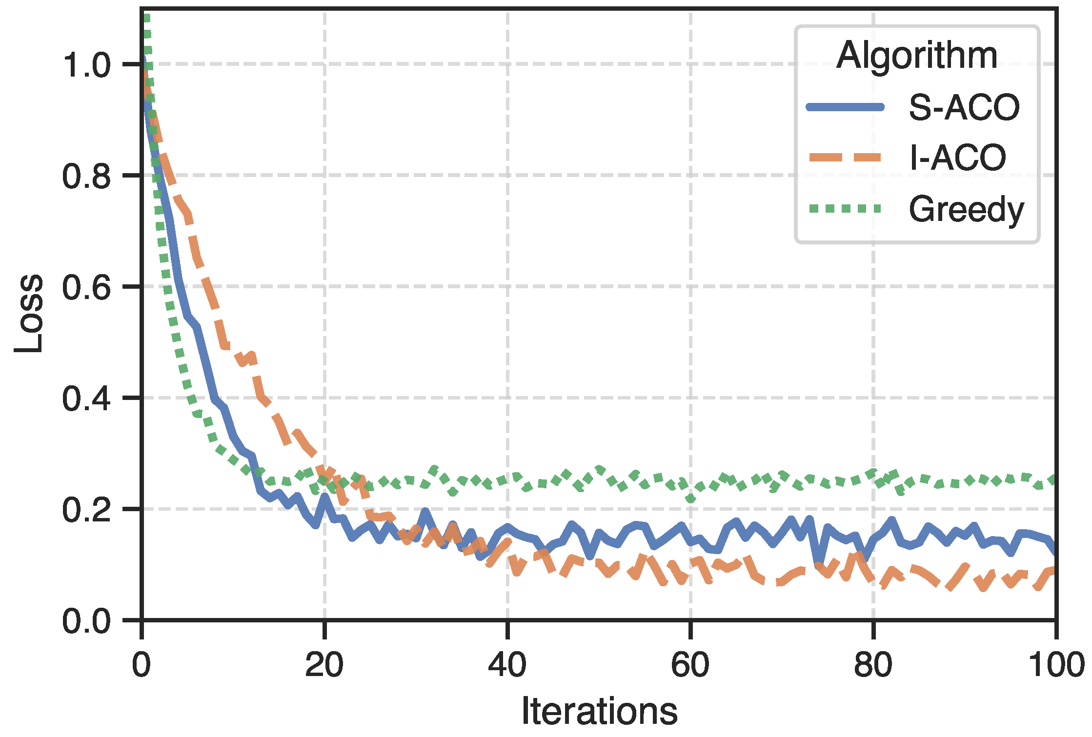
As shown in

Table 6. Performance Comparison of Different Algorithms for Active Localization Tasks. Lower values indicate better performance.

Algorithm	Avg. Comprehensive Cost ↓	Avg. Computation Time (ms) ↓
I-ACO (Proposed)	125.8	385.4
S-ACO	131.2	390.1
Greedy	155.4	45.2
RW	210.7	51.5

, I-ACO achieves the lowest average comprehensive cost of 125.8, representing a 4.1% performance improvement over S-ACO (131.2). Compared to the Greedy algorithm (155.4), the cost is reduced by 23.5%. These results indicate that the global optimization heuristic algorithm has significant advantages over local greedy strategies. The RW algorithm has the highest cost, confirming that unguided random search struggles to find high-quality solutions under complex constraints.

The convergence curves in Figure 1 (description based on text) reveal differences in algorithmic behavior. The I-ACO curve shows a smooth downward trend and plateaus only after a higher number of iterations, eventually converging to a lower cost value. This demonstrates that the MMAS pheromone boundary constraints (${\tau }_{min},{\tau }_{max}$) maintain search diversity, allowing the algorithm to escape local optima in later stages. The S-ACO curve descends rapidly in the early stages but quickly stagnates at a higher cost value. This is likely due to excessive pheromone accumulation on a suboptimal path, which halts the exploration of other paths. Therefore, this experiment proves that the improvements made to ACO are both effective and necessary.

5.4.2. Dynamic Performance Evaluation of Adaptive Switching Strategy

This experiment tests the performance of AAS under mixed task flows. The result is shown in

Table 7. Performance Comparison of AAS and Fixed Strategies under Mixed Task Flows.

Load Level	Metric	AAS (Proposed)	Fixed I-ACO	Fixed Greedy
Low Load	Success Rate (%)	100	100	100
	Avg. Cost	112.5	112.8	135.1
	Avg. Time (ms)	378.2	380.5	43.9
Medium Load	Success Rate (%)	100	100	98.5
	Avg. Cost	126.3	125.8	158.2
	Avg. Time (ms)	255.4	385.4	45.2
High Load	Success Rate (%)	99.2	82.5	93.4
	Avg. Cost	185.7	160.1	179.6
	Avg. Time (ms)	60.8	498.7	48.1

.

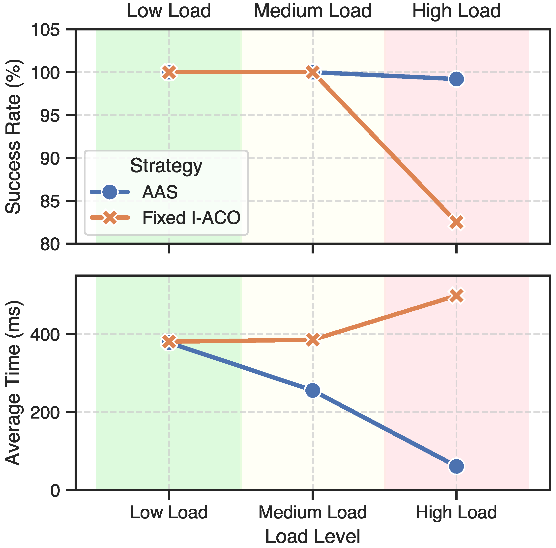
In the low load zone, the performance of AAS is almost identical to Fixed I-ACO, with both achieving high-quality solutions (cost approx. 112.5). This indicates that the AAS switching mechanism correctly selects the global optimization algorithm when resources are abundant.

In the medium load zone, the advantages of AAS begin to emerge. By switching to the ACO algorithm guided by historical utility, the average computation time is reduced from 385.4 ms (Fixed I-ACO) to 255.4 ms, an efficiency increase of 33.7%. To improve calculation speed, the solution cost increases slightly (from 125.8 to 126.3) but maintains high quality. This proves that historical utility value serves as highly efficient heuristic information, guiding the search to accelerate convergence while maintaining solution quality.

The high load zone embodies the greatest value of the AAS strategy. Under extreme resource tension and strict time constraints, the Fixed I-ACO scheduling success rate drops to 82.5% due to the time-consuming nature of its iterative search, with some tasks failing due to timeout. In contrast, AAS switches to the fast greedy algorithm based on historical utility, maintaining a success rate of 99.2%, which is comparable to the fastest Greedy algorithm (93.4%, noting that historical utility guidance makes finding feasible solutions more likely than pure greed). Although the cost of AAS (185.7) is slightly higher than Greedy (179.6) (likely due to different cost functions or local optima), it ensures service continuity with high reliability. This reflects the core philosophy of AAS design: optimization objectives change under different operating conditions, and scheduling reliability is prioritized under high load.

Figure 2 illustrates that as load shifts from low to high, the success rate of Fixed I-ACO drops significantly while computation time remains constant. Conversely, the AAS success rate remains high, and its computation time drops to a low level similar to Greedy when entering the high-load region, demonstrating AAS’s system load perception and dynamic decision-making capabilities.

5.4.3. Analysis of Long-Term Load Balancing Effects

This experiment validates the impact of each algorithm on overall system balance after long-term operation through simulation.

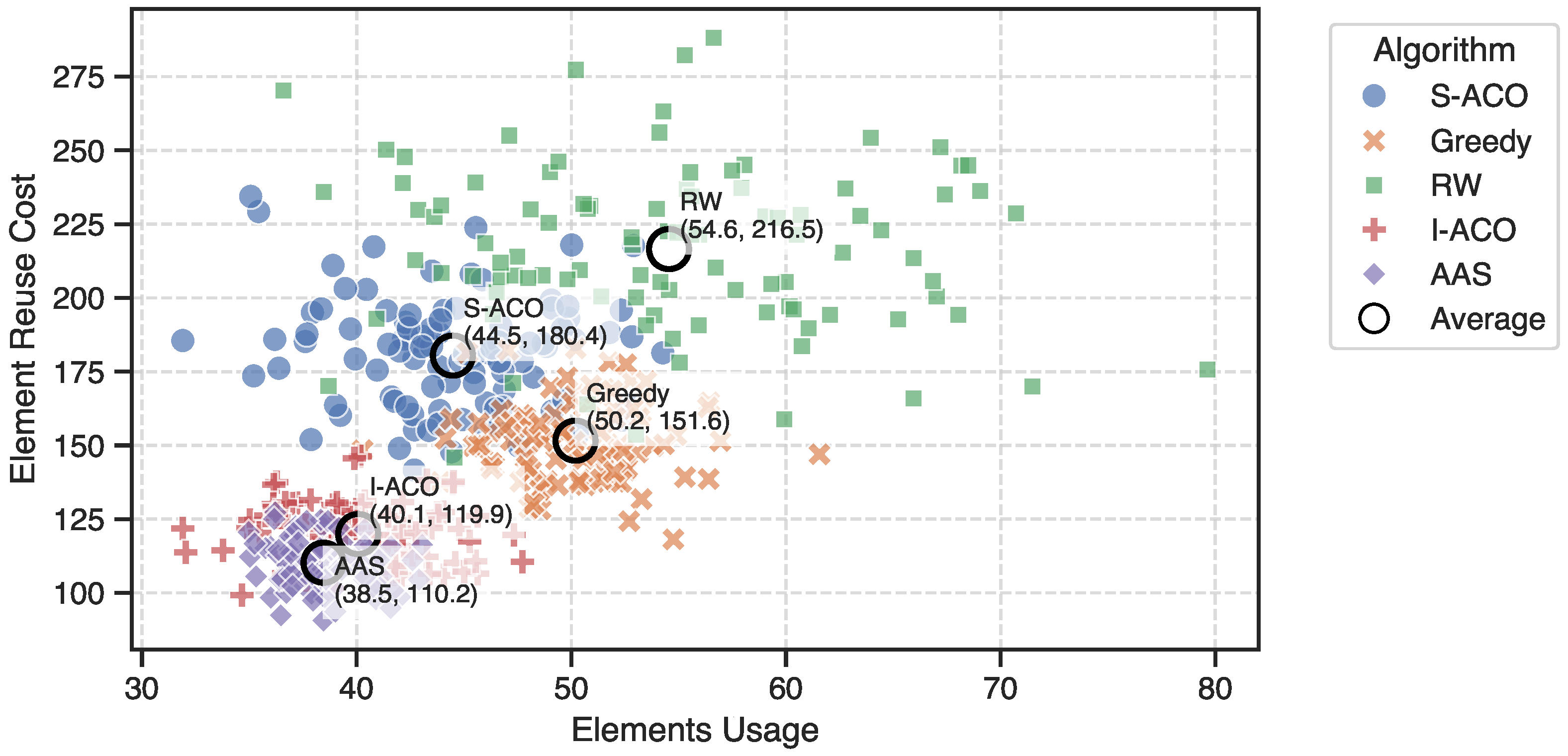
Figure 3 (description based on text) visually displays the trade-off between resource utilization efficiency (number of elements) and load balance (total reuse cost). The ideal solution is located in the bottom-left corner (few elements and low reuse cost). The scatter points for the AAS algorithm are mainly distributed near the ideal region, with an average point of (38, 110) close to the bottom left, indicating that AAS achieves a good balance between the two objectives. The I-ACO algorithm follows (average point 40, 120), with a relatively concentrated distribution but slightly inferior to AAS. S-ACO and Greedy show weaknesses in different objectives: S-ACO has high total reuse costs (avg. 180), while Greedy uses more elements (avg. 54). The RW algorithm has the most dispersed distribution, far from the ideal region.

This validates the multi-objective optimization capability of the AAS strategy. Through adaptive switching and utility value guidance, AAS reduces resource occupation (avg. 38 elements) and total reuse cost (avg. 110). This performance stems from AAS using I-ACO for global optimization at low loads, a hybrid strategy for accelerated convergence at medium loads, and switching to fast greedy at high loads, thereby finding scheduling solutions close to Pareto optimality in various scenarios.

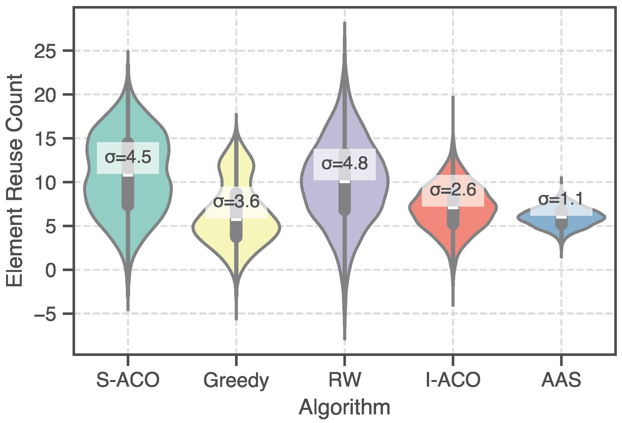
As shown in Figure 4 (description based on text), the violin plot for the AAS algorithm presents the narrowest symmetric distribution. Its standard deviation ($\sigma =1.1$) is lower than other algorithms, indicating that element reuse counts are highly concentrated around the mean (6 times), achieving optimal load balancing. The I-ACO violin plot follows ($\sigma =2.6$), suggesting that while the improved ACO possesses some load balancing capability, some elements still have high reuse counts. The violin plots for S-ACO and Greedy both exhibit bimodal distributions, indicating two classes of elements in the system: one with low reuse (S-ACO ≈ 8, Greedy ≈ 5) and another severely overloaded (S-ACO ≈ 15, Greedy ≈ 12). This “hotspot” effect reduces long-term system stability. The RW algorithm has the widest plot ($\sigma =4.8$) and the most dispersed reuse distribution, failing to achieve load balancing. This result verifies the long-term value of the AAS strategy. By utilizing adaptive switching and historical utility guidance, AAS optimizes the quality of individual schedules and avoids resource fragmentation and hotspot formation through a historical learning mechanism.

6. Conclusions

To address the complex resource scheduling challenges in large-scale digital array radar systems, this paper proposes a novel framework integrating graph-theoretic modeling with adaptive heuristics. We formulated the multi-beam scheduling problem as a constrained connected subgraph optimization task and developed an I-ACO algorithm. By incorporating pheromone boundary constraints and elite strategies, I-ACO effectively balances exploration and exploitation. Furthermore, an AAS strategy was introduced to dynamically select optimal algorithms based on real-time load, resolving the conflict between solution quality and response speed.

Experimental results demonstrate the method’s superiority. I-ACO reduced solution costs by up to 23.5% compared to greedy baselines. Crucially, the AAS strategy maintained a 99.2% scheduling success rate under high-load conditions and improved long-term load balancing by 41.5%, effectively guaranteeing system QoS across six heterogeneous task types.

Although our current work focuses on validating the logic and scalability of the proposed I-ACO and AAS strategies under extreme load conditions that are difficult to reproduce safely in field tests, future work will involve collaboration with industry partners to implement and test these algorithms in real-world digital array radar systems. This will allow us to assess their practical performance, robustness, and adaptability in operational environments. Additionally, we will also develop adaptive mechanisms to learn optimal LUR thresholds based on real-time performance feedback, enhancing the method’s applicability across diverse scenarios.

References

1. Luo, X.; Chen, H.H.; Guo, Q. LEO/VLEO Satellite Communications in 6G and Beyond Networks–Technologies, Applications, and Challenges. IEEE Netw. 2024, 38, 273–285. [Google Scholar] [CrossRef]
2. Norp, T.; Fine, J.Y.; Djapic, R. Network aspects of integrating 5G and satellite communication. Int. J. Satell. Commun. Netw. 2023, 41, 239–248. [Google Scholar] [CrossRef]
3. S U, Y.; Cheng, T.; He, Z.; Li, X.; Lu, Y. Adaptive resource management for multi-target tracking in co-located MIMO radar based on time-space joint allocation. J. Syst. Eng. Electron. 2020, 31, 916–927. [Google Scholar] [CrossRef]
4. Xu, G.; Shan, G.; Duan, X. Sensor scheduling for ground maneuvering target tracking in presence of detection blind zone. J. Syst. Eng. Electron. 2020, 31, 692–702. [Google Scholar] [CrossRef]
5. Ma, R.; Ma, Y.; Lin, Z.; Ma, Y.; Yang, W.; Dusit, N. Covert Communication Assisted by Movable Time-Modulated Arrays. IEEE Commun. Lett. 2026, 30, 382–386. [Google Scholar] [CrossRef]
6. Phuong T., T.; Thong-Nhat, T.; Ba Cao, N.; Tran Manh, H.; Le The, D.; Taejoon, K. Enhancing Secrecy Performance of Full-Duplex Relaying Systems Using IRS and RSMA. IEEE Trans. Mob. Comput. 2026, 25, 878–891. [Google Scholar] [CrossRef]
7. Hu, B.; Zhu, Y.; Zhou, Y. Simulated annealing whale radar resource scheduling algorithm based on Cauchy mutation. J. Northwest. Polytech. Univ. 2022, 40, 796–803. [Google Scholar] [CrossRef]
8. Caleb, F.; Mark, Y.; Daniel, T.; John, L.; Adam, M. Digital Phased Arrays: Challenges and Opportunities. Proc. IEEE 2016, 104, 487–503. [Google Scholar] [CrossRef]
9. Yi, W.; Yuan, Y.; Liu, G.; Ge, J.; Kong, L.; Yang, J. Recent Advances in Multi-radar Collaborative Surveillance: Cognitive Tracking and Resource Scheduling Algorithms. J. Radars 2023, 12, 471. [Google Scholar] [CrossRef]
10. Han, R.; Sun, Z.; Wang, J. Multi-radar Collaborative Task Assignment Algorithm Based on Swarm Intelligence Optimization. Mod. Radar 2025, 47, 53–56. [Google Scholar] [CrossRef]
11. Qi, K.; Dong, Z.; Zhou, Y.; Yi, L.; Feng, X.; Qin, P. Multi-beam forming algorithm of phased array for GEO fully-flexible satellites. Space Electron. Technol. 2025, 22, 37–43. [Google Scholar] [CrossRef]
12. Han, X.; Sun, Q.; Shu, T.; Tang, B.; Yu, W. A Study on the Anti-jamming Test and Evaluation of Airborne Active Phased Array Radar. Mod. Radar 2017, 39, 91–96. [Google Scholar] [CrossRef]
13. Zuo, L.; Hu, J.; Sun, H.; Gao, Y. Resource allocation for target tracking in multiple radar architectures over lossy networks. Signal Process. 2023, 208, 108973. [Google Scholar] [CrossRef]
14. Xie, Q.; Wang, Z.; Wen, F.; He, J.; Truong, T.K. Coarray Tensor Train Decomposition for Bistatic MIMO Radar With Uniform Planar Array. IEEE Trans. Antennas Propag. 2025, 73, 5310–5323. [Google Scholar] [CrossRef]
15. Xie, Q.; Shi, J.; Wen, F.; Zheng, Z. Higher-order tensor decomposition for 2D-DOD and 2D-DOA estimation in bistatic MIMO radar. Signal Process. 2026, 238, 110196. [Google Scholar] [CrossRef]
16. Ding, L.; Shi, C.; Zhou, J. Collaborative route optimization and resource management strategy for multi-target tracking in airborne radar system. Digit. Signal Process. 2023, 138, 104051. [Google Scholar] [CrossRef]
17. Qi, C.; Xie, J.; Zhang, H. Joint Antenna Placement and Power Allocation for Target Detection in a Distributed MIMO Radar Network. Remote Sens. 2022, 14, 2650. [Google Scholar] [CrossRef]
18. Zhou, B.; Chen, F. Graph-Structured Sparse Optimization for Connected Subgraph Detection. In Proceedings of the 2016 IEEE 16th International Conference on Data Mining (ICDM), Barcelona, Spain, 12–15 December 2016; pp. 709–718. [Google Scholar] [CrossRef]
19. Daniel, R.; Henriette, F.; Thorsten, K. Optimal connected subgraphs: Integer programming formulations and polyhedra. Networks 2022, 80, 314–332. [Google Scholar] [CrossRef]
20. Mohammed, E.K.; Gunnar, W.K. Solving the Maximum-Weight Connected Subgraph Problem to Optimality. arXiv 2014, arXiv:1409.5308. [Google Scholar] [CrossRef]
21. Mohamed, H.; Nelson, M.; Mehdi, M. Enhanced compact models for the connected subgraph problem and for the shortest path problem in digraphs with negative cycles. Comput. Oper. Res. 2013, 40, 2485–2492. [Google Scholar] [CrossRef]
22. Cesare, V. A genetic approach to the maximum common subgraph problem. In Proceedings of the CompSysTech ’19: 20th International Conference on Computer Systems and Technologies, Ruse, Bulgaria, 21–22 June 2019; Association for Computing Machinery: New York, NY, USA; pp. 98–104. [Google Scholar] [CrossRef]
23. Joseph L, P.; Nongmeikapam Brajabidhu, S.; Laiphrakpam Dolendro, S.; Anish Kumar, S. Solving Dense Subgraph Problems Using Genetic Algorithm. In Proceedings of the TENCON 2023–2023 IEEE Region 10 Conference (TENCON), Chiang Mai, Thailand, 31 October–3 November 2023; pp. 674–679. [Google Scholar] [CrossRef]
24. Jorge, C.O.; María C., G.F.; Christian, R.M. Genetic algorithm and edge-colorings of complete graphs with connected classes. arXiv 2024, arXiv:2405.01811. [Google Scholar] [CrossRef]
25. Alberto, F.; Thomas, S. Revisiting simulated annealing: A component-based analysis. Comput. Oper. Res. 2019, 104, 191–206. [Google Scholar] [CrossRef]
26. Dahmri, H.; Bouamama, S. A Simulated Annealing-Based Multiobjective Optimization Algorithm for Minimum Weight Minimum Connected Dominating Set Problem. arXiv 2024, arXiv:2312.11527. [Google Scholar]
27. Zoltán, T.; Noémi, G. An Ant Colony Optimisation Approach to the Densest k-Subgraph Problem*. In Proceedings of the 2022 24th International Symposium on Symbolic and Numeric Algorithms for Scientific Computing (SYNASC), Hagenberg/Linz, Austria, 12–15 September 2022; pp. 208–211. [Google Scholar] [CrossRef]
28. Souza Almeida, L.; Goerlandt, F. An ant colony optimization approach to the multi-vehicle prize-collecting arc routing for connectivity problem. Multimodal Transp. 2022, 1, 100033. [Google Scholar] [CrossRef]
Figure 1. Convergence curves of the cost function for different algorithms during the solution process.
Electronics 15 00088 g001
Figure 2. Perfomance of AAS and Fixed I-ACO under varying system loads.
Electronics 15 00088 g002
Figure 3. Scatter plot of element reuse cost vs. number of elements used.
Electronics 15 00088 g003
Figure 4. Distribution of element reuse counts after long-term simulation.
Electronics 15 00088 g004