Article

A Modification Method for Domain Shift in the Hidden Semi-Markov Model and Its Application

1
Graduate School of Information Science and Technology, Hokkaido University, Sapporo 060-0808, Japan
2
Faculty of Information Science and Technology, Hokkaido University, Sapporo 060-0808, Japan
3
Kanagawa Institute of Industrial Science and Technology, Ebina 243-0435, Japan
4
Faculty of Environment and Information, Yokohama National University, Yokohama 240-8501, Japan
5
National Institute of Advanced Industrial Science and Technology, Koto-ku, Tokyo 135-0064, Japan
*
Author to whom correspondence should be addressed.
Electronics 2025, 14(8), 1579; https://doi.org/10.3390/electronics14081579
Submission received: 25 February 2025 / Revised: 31 March 2025 / Accepted: 10 April 2025 / Published: 13 April 2025

Abstract

:
In human behavior recognition using machine learning, model performance degrades when the training data and operational data follow different distributions which is a phenomenon known as domain shift. This study proposes a method for domain adaptation in the hidden semi-Markov model (HSMM) by modifying only the emission probability distributions. Assuming that the state transition probabilities remain unchanged, the method updates the emission probabilities based on the posterior distribution of the target domain. This approach enables domain adaptation with minimal computational cost without requiring model retraining. The effectiveness of the proposed method was evaluated on synthetic time-series data from different domains and actual care work data, achieving recognition performance comparable to that of models retrained for each domain. These findings suggest that the proposed method applies to various time-series data analysis tasks requiring domain adaptation.

1. Introduction

Pattern recognition methods based on machine learning have been widely used in human behavior recognition [1,2,3]. Most of these machine learning systems are trained using accumulated training data, and it is generally assumed that the operational data follows the same independent and identically distributed (i.i.d.) assumption as the training data. However, this assumption does not always hold, meaning that the performance of the system degrades when the training and test data follow different probability distributions. For example, in a model for recognizing images of dogs, if the training data are an image of a dog in a grassland, while the test data attempts to recognize a dog indoors or in water, the accuracy is reduced. This issue is known as out-of-distribution (OOD) generalization [4], and ensuring the performance of a trained model without additional adaptation is challenging [5,6]. In particular, behavior recognition tasks are significantly affected by variations in environments and individual differences, making this problem a critical challenge.
Situations where the i.i.d. assumption does not hold are often referred to as domain shift or distribution shift. To address this, domain adaptation (DA) techniques have been proposed, which aim to compensate for the distribution mismatch between the source and target domains [7,8,9], and various DA approaches exist. Divergence-based DA learns domain-invariant feature representations by minimizing the distributional distance between the source and target domain data [10,11,12]. Adversarial learning-based DA employs a discriminator to distinguish whether a given sample belongs to the source or target domain [13,14,15], while a feature extractor for the target domain is trained adversarially against the discriminator [16]. Reconstruction-based DA utilizes auxiliary reconstruction tasks to construct shared feature representations across domains [17,18,19]. There are also methodologies such as transition learning and fine-tuning as a broader framework for machine learning with data following different distributions [20]. However, most of these approaches require a high computational cost every time the target domain changes, because they require parameter optimization via model retraining. Therefore, we propose domain adaptation with a very fast computation time by directly correcting the parameters.
In this study, we propose a method to adapt the hidden semi-Markov model (HSMM) [21] to the target domain by modifying its parameters. Conventional behavior recognition methods primarily focus on identifying specific activities from observation data using pattern recognition approaches. However, as the scope of behavior recognition expands, there is growing interest in analyzing the latent factors and structural characteristics underlying human activities. From this perspective, models such as the hidden Markov model (HMM) [22] and HSMM, which explicitly consider latent state transitions, are promising techniques and have been widely applied in various behavior recognition and analysis tasks [23,24,25,26,27]. The authors have applied an HSMM to care work recognition, which classifies which care works are performed by care workers [28,29]. Our research identified that differences in work environments within care facilities can degrade recognition accuracy, highlighting the need for domain adaptation in activity recognition models.
Many tasks consist of a series of sequential elemental tasks. For example, care work consists of multiple elemental tasks that are sequentially performed to complete an overall task. The order of elemental tasks is determined regardless of the domain, such as the work environment. In modeling, such tasks with HMM or HSMM, transitions from one elemental task to the next can be interpreted as transitions between hidden states, suggesting that hidden states correspond to elemental tasks. Thus, if the sequence of elemental tasks remains unchanged despite variations in the work environment, it can be hypothesized that the state transition probabilities of the Markov model are domain invariant. Based on this hypothesis, our method achieves domain adaptation at a very low computational cost by assuming that the state transitions are the same between the source and target domains and correcting only the output probability distribution. In experiments, the authors evaluated the effectiveness of the proposed method by correcting the parameters for artificial data with different distributions. In addition, the transfer of a care receiver from a bed to a wheelchair, one of the care tasks, was measured in different environments to verify the effectiveness of the proposed method on actual data.

2. Methods

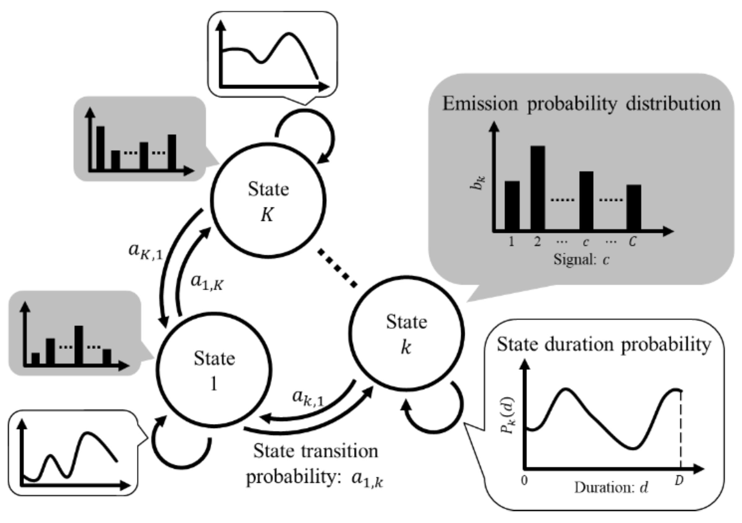
2.1. Outline: Pattern Recognition of HSMM

The hidden Markov Model is defined as a model in which states (signal sources) with arbitrary probability density functions are connected by a first-order Markov chain. In contrast, the hidden semi-Markov model introduces a state duration probability P j ( d ) ( j = 1 , , K , d = 1 , , D ) for each state, allowing the model to incorporate time dependencies in state transitions. K denotes the number of states, and D denotes the maximum state duration length in the HSMM. Figure 1 shows a schematic diagram of HSMM. In this study, the authors adopt the explicit duration HMM (ED-HMM), a simple form of HSMM [30]. Given observed time-series data O = { o t } t = 1 , , T , the likelihood at time step t is computed as follows:
α t ( j ) = i = 1 K d = 1 D α t d ( i ) a i , j P j ( d ) u t ( j , d )
u t ( j , d ) = τ = t d + 1 t b j ( o τ )
where the initial condition is given by α 1 ( j ) = π j P j ( 1 ) b j ( o 1 ) . Here, π j ( j = 1 , , K ) denotes the initial state probability, A = { a i , j } j = 1 , , K i = 1 , , K denotes the state transition probability matrix indicating the probability of transitioning from state i to state j at the next time step ( a i , i = 0 , i = 1 , , K ), and b j ( o t ) denotes the probability that o t is emitted from state j at time t. Thus, the likelihood function for the entire observed time-series data p ( O | θ ) is as follows:
p ( O | θ ) = j = 1 K α T ( j )
In this study, the authors model the emission probability distributions b k ( · ) of each state using a categorical distribution defined as b j ( o t = c ; ϕ k ) = ϕ k , c . Here, ϕ k = ϕ k , 1 , , ϕ k , C denotes the parameter set of the categorical distribution for state k, and ϕ k , c denotes the emission probability of event c. The parameters satisfy the constraints ϕ k , c 0 , c = 1 C ϕ k , c = 1 . By identifying the model parameters θ = { π k , A , P k , ϕ k } k = 1 , , K , we can estimate the transitions of the hidden states that are not directly observable from the observed time-series data. The estimated hidden state sequence S ^ = { s t ^ } t = 1 , , T is given as follows:
s ^ t = arg max 1 j K α t ( j )
using α t used in the likelihood calculation. From the distribution ϕ k , we can interpret the event that each state represents. The state transition order of the latent variable can be inferred from A , while the duration of each latent variables can be inferred from P k . By analyzing the estimated hidden state sequence S ^ , we can visualize the temporal variations of the latent factors embedded in the observed time-series signal. Furthermore, pattern recognition can be performed using the likelihood function p ( O | θ ) .

2.2. Modification of Emission Probability Distributions

In the proposed method, we assume that the latent factors of the data, namely the state transition probabilities and state duration probabilities, remain unchanged even when the domain differs. Thus, only the emission probability distribution ϕ is modified. First, an HSMM is trained using the observed data O source from the source domain and obtain the model parameters θ source . By identifying θ source for O source , hidden state sequence S ^ source is estimated, which represents the latent changes in the observed data. Assuming that state transitions are identical between the source and target domains, we further assume that the hidden state sequence S ^ target of the observed data O target from the target domain undergoes the same transitions as in the source domain. In other words, the we introduce the assumption that the match rate m between the hidden state sequences of the two domains, defined by the following Equation (5), is equal to 1.
m = t = 1 T δ ( s ^ t source , s ^ t target ) T
where δ ( x , y ) denotes the Kronecker delta, which is defined as δ ( x , y ) = 1 if x = y , and δ ( x , y ) = 0 otherwise.
During the training process of HSMM, the emission probability distributions ϕ is updated to maximize the following function (6).
Q ( θ old , ϕ ) = S P ( S | O ; θ old ) t = 1 T log ϕ s t , o t
where θ old represents the parameters before updating. However, when the assumption m = 1 holds, meaning that S ^ target is known for O target , the conditional probability is as follows:
P ( S | O ; θ old ) = 1 ( S = S ^ target ) 0 ( otherwise )
and Equation (6) becomes as follows.
Q ( θ old , ϕ ) = t = 1 T log ϕ s t , o t
The emission probability distributions that maximize this function are defined as the new categorical distributions parameter for the target domain, denoted as ϕ k target = ϕ k , 1 target , , ϕ k , C target . Applying the Lagrange multiplier method under the constraint c = 1 C ϕ k , c L = 1 , the modified emission probability distributions are as follows.
ϕ k , c target = t = 1 T δ ( s ^ t target , k ) δ ( o t target , c ) t = 1 T δ ( s ^ t target , k )
In Equation (9), the denominator represents the number of times states k occur in the hidden state sequence S ^ target corresponding to the observed time-series data O target . The numerator represents the number of occurrences where both state k and observation symbol c are observed simultaneously. That is, the new emission probability distributions are obtained by frequency counting. Therefore, given observation data of length T, the computational complexity required to modify the emission probability distributions by the proposed method is K T . The flow of emission probability distribution modification using the proposed method is shown in Figure 2.

3. Experiments and Results

3.1. Experimental Setup
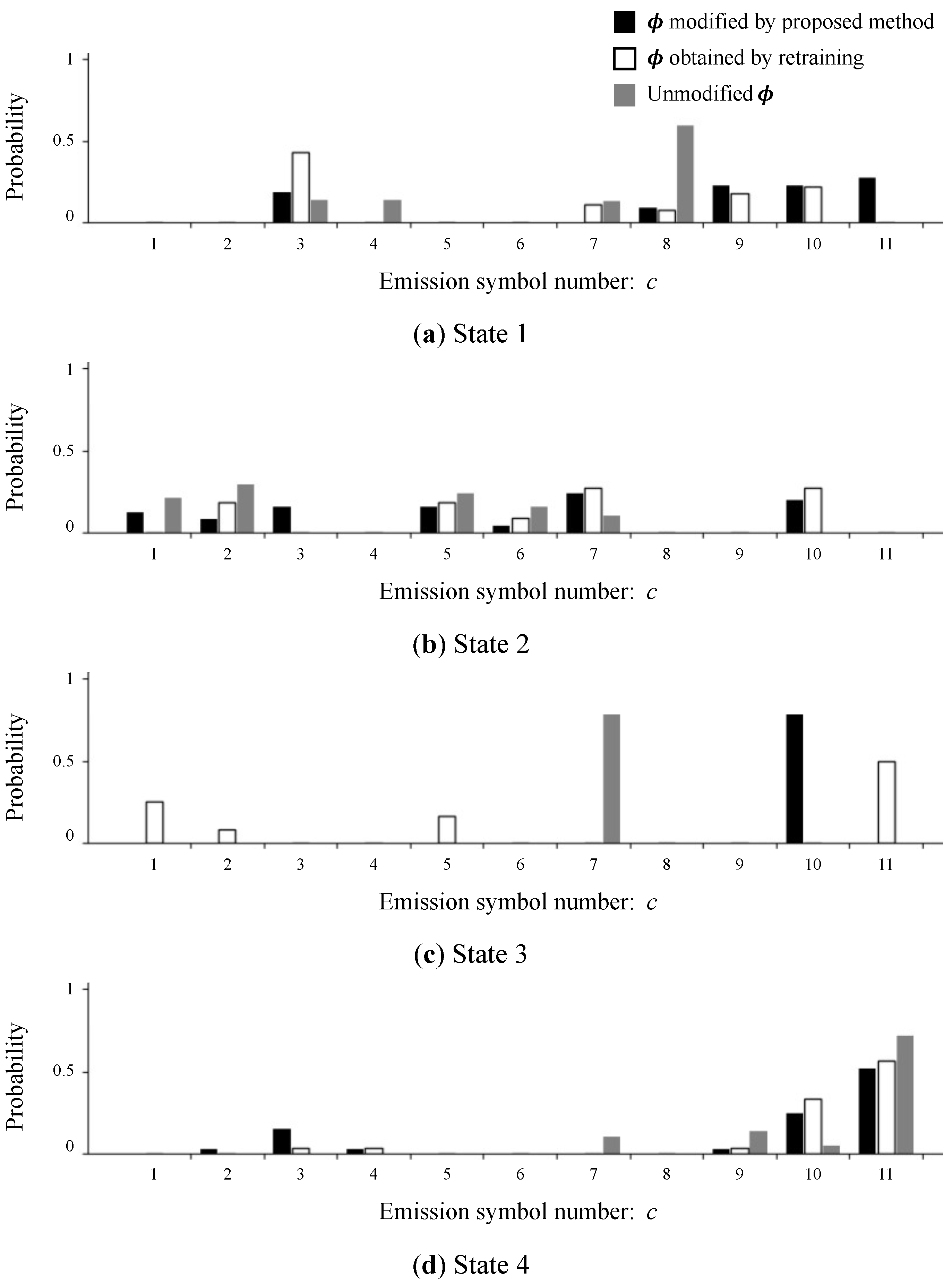
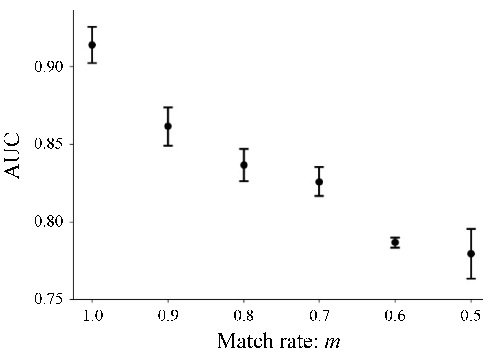
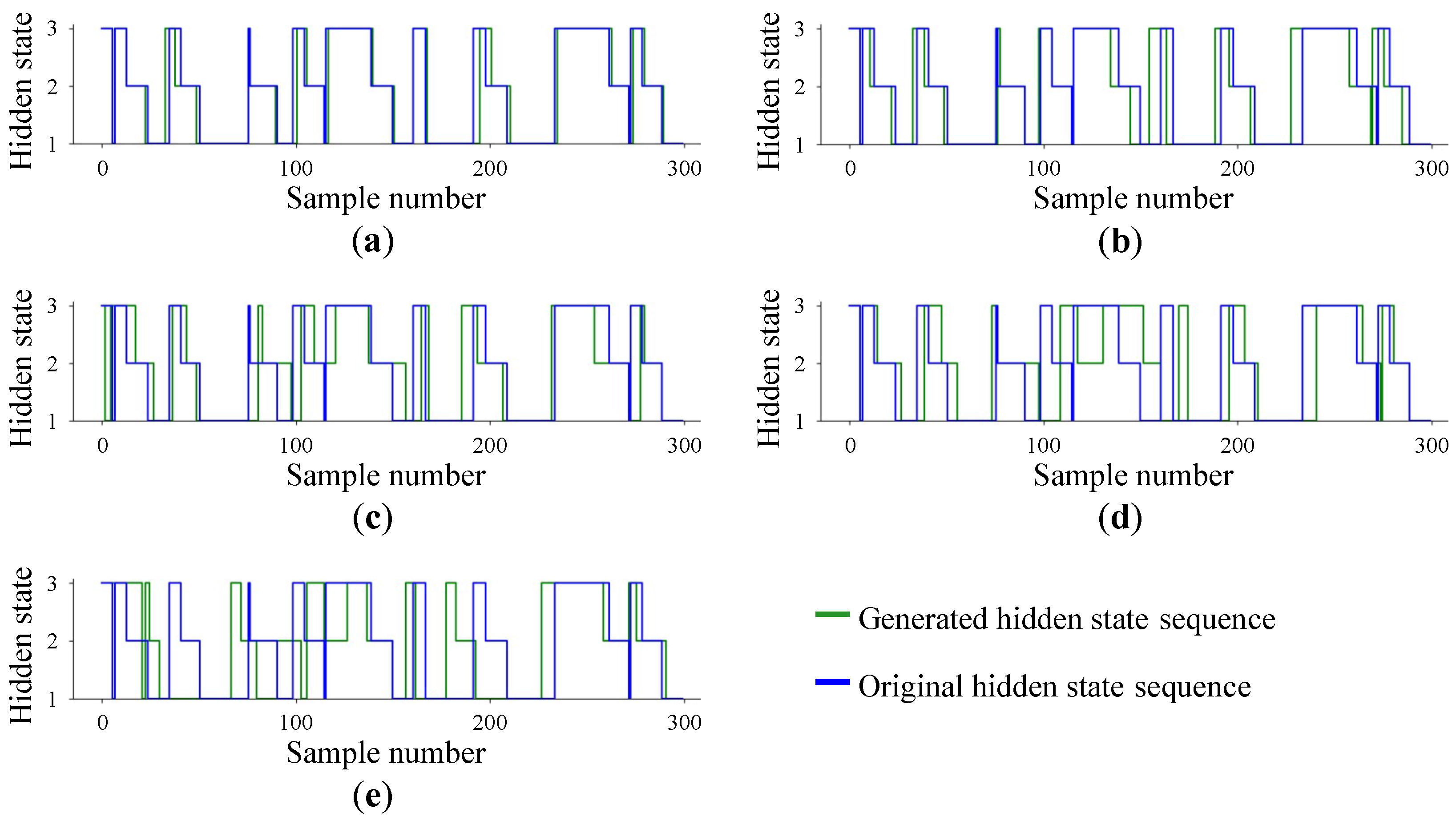
To evaluate the performance of the proposed method, we conducted a time-series pattern analysis using synthetic data. In this experiment, we used one-dimensional time-series signals generated from two different ED-HMMs, which had distinct emission probability distributions but shared the same hidden state transition. One time-series dataset was used for training the model, while the other was used for modifying the emission probability distributions. These two time-series datasets were generated from ED-HMM with the number of states: 3, the maximum state duration: 30, and the number of output symbols: 6. Usually, the number of states in a hidden semi-Markov model is modeled as less than the number of symbols. In this experiment, the above parameters were chosen for ease of analysis. The model parameters θ were generated using uniform random values. For evaluation, a one-dimensional time-series dataset was constructed by concatenating signals generated using multiple ED-HMMs. Specifically, in addition to the ED-HMM used for generating the correction data, two additional ED-HMMs with different parameters were employed.
To obtain a sufficient amount of data for output probability distribution correction in all states, we used 300 samples of training data and trained the model with the number of states: K = 3 and maximum state duration: D = 30 during training. After training, the hidden state sequence of the training data were estimated using the trained model. The estimated hidden state sequence was used to apply parameter modifications via the proposed method. For evaluation, we prepared a dataset containing 300 samples. The datasets consisted of 160 samples generated from the same ED-HMM that produced the data for modification, representing the data in the target domain. Additionally, 70 samples were generated from each of the two ED-HMM with random parameters using uniform random values, and these samples were concatenated before and after the data in the target domain. The characteristics of each data set are shown in the Table 1. To assess the model’s performance, the log-likelihood was computed using Equation (3) and normalized so that the minimum value was 0 and the maximum value was 1. The area under the curve (AUC) of the normalized log-likelihood was then calculated. As baselines, we compared the proposed method with a model trained on the modification data as training data and a model without any parameter correction.

3.2. Results

Figure 3 presents the categorical distributions, modified by the proposed method, the ED-HMM that generated the data for modification, unmodified. Table 2 presents the cosine similarity between the categorical distributions modified by the proposed method and the categorical distributions of the ED-HMM that generated the data for modification. The results indicate that the proposed method successfully modified the distribution to match the categorical distribution of the data for modification.
Figure 4 illustrates the log-likelihood of the validation data for the modified model using the proposed method and the retrained model with the data for modification as the training data and the original model without parameter modification. The gray region in Figure 4 represents the segments of the validation data generated by the ED-HMM used for correction data generation. An increase in likelihood within this region indicates successful pattern recognition. The results show that only the model corrected by the proposed method and the retrained model successfully recognized the patterns. Table 3 presents the AUC and Table 4 presents the precision, recall, and F1-score for the validation data of each model, serving as a measure of recognition accuracy. AUC values closer to 1 indicate higher recognition accuracy, while values near 0.5 suggest that recognition is nearly random. The results confirm that the proposed method achieves recognition performance comparable to the retrained model, demonstrating its effectiveness. Additionally, the model without parameter correction exhibited nearly random classification performance, highlighting the necessity of adapting the model to domain shift.

4. Discussion and Application

4.1. Discussion

The number of states affects the domain adaptation performance of the proposed method if the assumption that state transitions do not vary across domains is not partially valid. The higher the number of states, the more patterns of hidden state sequences that can be taken, and the larger the difference in state transitions between domains is expected to be. Other hyperparameters, such as maximum state duration length, have little effect on the domain adaptation performance of the proposed method. However, if the hyperparameters are not properly set, they may have a negative impact on HSMM pattern recognition.
We discuss the computational cost of the proposed method as a framework that eliminates the need for retraining when adapting models to domain shifts. The computational complexity of the proposed method is O ( K T ) , while that of ED-HMM training is O ( K 2 D T ) . This suggests that the proposed method is particularly advantageous as the number of states increases. Figure 5 presents the computation time required for modification using the proposed method and retraining of ED-HMM, under varying dataset sizes and state numbers. The datasets used for modification and training were generated by an ED-HMM with uniform random values, with a maximum state duration of 50. The dataset size and the number of states were varied, and the computation time was measured. The vertical scales in Figure 5 show that the proposed method significantly reduces the computation time. The proposed method can perform fast domain adaptation in less than 0.1 s even when the number of samples exceeds 10,000. Retraining, on the other hand, increased the learning time to nearly 1 min as the amount of data increased. In addition, as can be seen from the computational complexity, the retraining increases the computation time exponentially with the number of states K, while the proposed method increases the computation time linearly for all hyperparameters. Furthermore, since ED-HMM training results depend on initial values, it is common practice to train multiple models with different random initial values and select the best-performing one. Therefore, the actual training time for ED-HMM is expected to be several times longer than this analysis. In contrast, the proposed method does not require setting initial values and can uniquely modify the output probability distribution. Therefore, the proposed method is computationally inexpensive, even though there is no randomness in the results and the optimal model can be obtained with a single adaptation.
The proposed method with model retraining and other domain adaptation methods were compared. Table 5 summarizes the characteristics of each method. The proposed method is able to perform domain adaptation much faster than other methods and requires less data to correct the emission probability distribution. Furthermore, when the precondition that the state transitions are consistent across domains is satisfied, the performance of the proposed method is equivalent to model retraining. However, if this precondition does not hold, performance is expected to deteriorate. While model retraining is computationally expensive and requires a very large amount of data, it is also highly efficient. Fine tuning based on trained models can reduce the computational cost and amount of data compared to re-training. GAN-based domain adaptation, which creates feature extractors that do not vary across domains through adversarial generation, is difficult to train feature extractors, but has the potential to acquire high-performance models at relatively low cost. These facts make the proposed method a very fast domain adaptation compared to other domain adaptation techniques. In general, domain adaptation requires changing the model each time the target domain changes, which requires computation time and data for adaptation each time. Therefore, the proposed method is very effective when the target domain changes frequently. However, since the accuracy of the proposed method is somewhat lower than other methods, the disadvantages of misrecognition and the cost of modifying records should be considered.

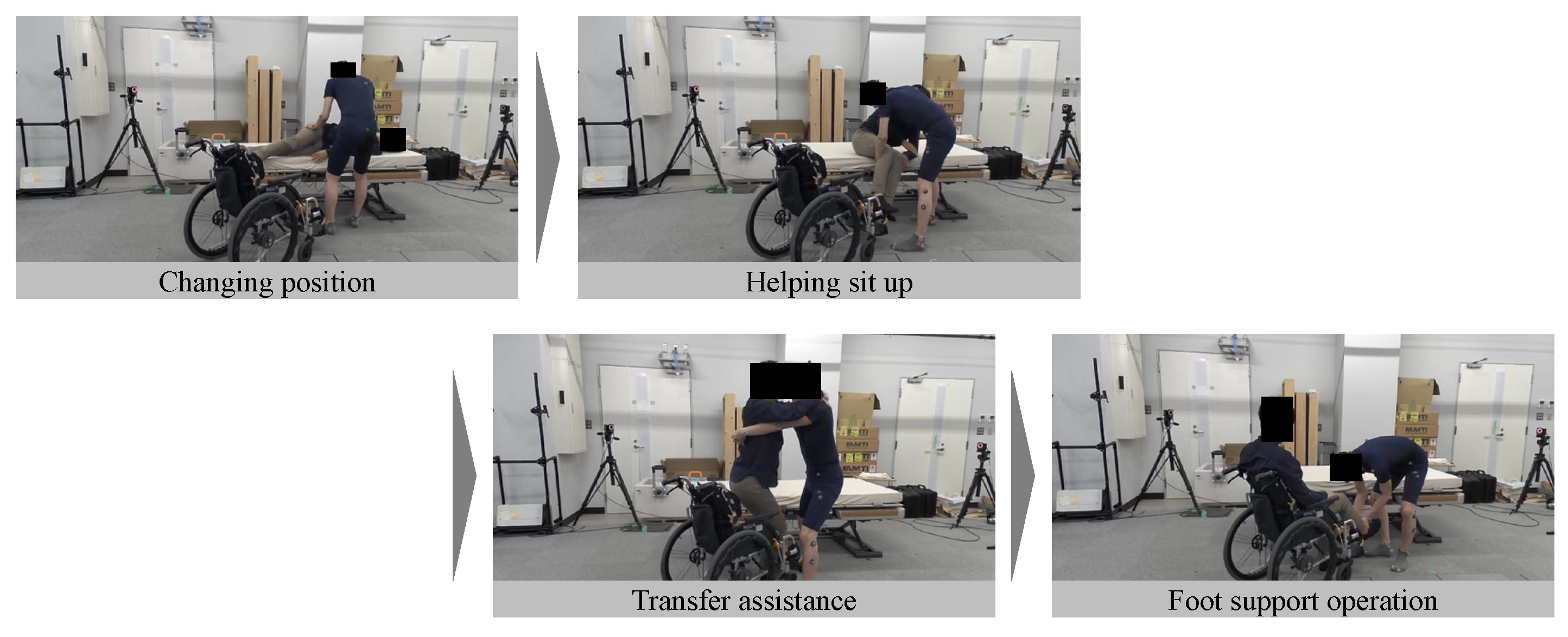
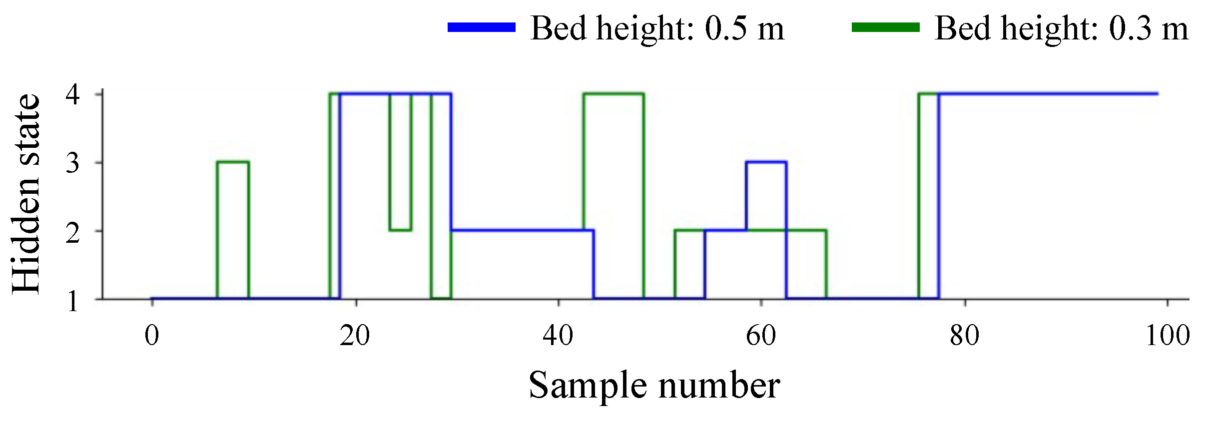
4.2. Application for Care Work Recognition

To evaluate the effectiveness of the proposed method on actual data, the authors conducted pattern recognition on motion data recorded during care work. Care work consists of multiple elemental tasks that are sequentially performed to complete an overall task. Figure 6 illustrates an example of a transfer assistance task, in which a care worker moves a care recipient from a bed to a wheelchair. By interpreting the transition from one elemental task to the next as state transitions, it is possible to model care work using an HSMM. In care environments, various factors such as the positioning and size of assistive equipment and the degree of independence of the care recipient introduce variability. However, the order of elemental tasks, as shown in Figure 6, is expected to remain largely unchanged, meaning the state transitions should also be relatively stable. On the other hand, posture angles and accelerations of the care worker, which are used as feature signals for the recognition model, are significantly affected by changes in the work environment, potentially degrading recognition accuracy.
In the experiment, two different work environments with varying bed heights were examined to evaluate the effect of domain differences. The experimental setup is shown in Figure 7. In the experiment, a nursing care bed and a wheelchair were used, and the transfer assistance tasks from the bed to the wheelchair were measured, as shown in Figure 6. The subjects were males in their 20 s with no previous caregiving experience for either the caregiver or the assisted caregiver. For model training, motion data measured in an environment where the bed height was set to 0.3 m were used. For model evaluation, we used data from an environment with a bed height of 0.5 m, where transfer assistance tasks were performed three times. The measured motions were categorized into the list of upper and lower body motion shown in Table 6. A suitable label c 1 , , C was assigned to each motion pair, which was then used as a feature value for ED-HMM. Annotations were performed every 0.2 s based on visual inspection. Since the duration of each trial varied, the total number of samples was normalized to 100 per trial.
For model training, we used three trials of transfer assistance tasks measured in an environment with a bed height of 0.5 m. The model parameters were set with the number of states as 4 and the maximum state duration as 50. Among the trained parameters θ source , the emission probability distributions were modified using two trials of data measured in the environment with a bed height of 0.3 m, following the proposed method. The remaining trial was used as evaluation data, and the likelihood of the entire evaluation data was computed to assess the feasibility of work recognition.
Figure 8 compares the categorical distributions: modified using the proposed method, obtained by retraining the model using the data for modification as training data, unmodified. For retraining, the categorical distribution of the model trained with the 0.5 m bed height data were used as the initial values to maintain label consistency. Table 7 presents the cosine similarity between the categorical distributions modified by the proposed method and the categorical distributions obtained by retraining. The results show that for states 1, 2, and 4, the proposed method yielded categorical distributions similar to those obtained through retraining. In particular, for state 4, the distributions were nearly identical. However, in state 3, the categorical distribution obtained via the proposed method differed from that obtained via retraining. This discrepancy is likely due to the optimization process in retraining producing an extreme categorical distribution. As shown in Figure 8c, the retrained categorical distribution assigns a probability of 1 to symbol 10, effectively making the symbol equivalent to the hidden state. This indicates that the number of states set as hyperparameters was too large to obtain an appropriate model. It is possible to obtain a higher-performance model by setting the hyperparameters appropriately.
Figure 9 presents the log-likelihoods for the entire evaluation data using four models: the proposed method, the retrained model using θ source as initial values, the retrained model with random initial values(trained 10 times), and the unmodified original model. The results show that the performance of the model modified using the proposed method falls within the range of the randomness of retrained models. This confirms that the proposed method reduces computational costs while achieving recognition performance comparable to that of a retrained model. Furthermore, in the unmodified original model, underflow occurred in likelihood computation, rendering work recognition infeasible. This highlights the necessity of optimizing model parameters to account for changes in the work environment.
Finally, the authors examined how well the hidden state transitions aligned between different domains in the actual data. Figure 10 shows the estimated hidden state sequences for the two environments. The results indicate that, despite domain differences, the transition patterns of hidden states remained similar. This supports our hypothesis that hidden state transitions do not change significantly across different domains. The match rate of the two hidden state sequences in Figure 10 was found to be m = 0.73 . According to the results in Figure 11, when the match rate is approximately 0.7, the recognition performance is about 90% of that achieved by a retrained model, demonstrating that pattern recognition remains feasible. These findings partially demonstrate the effectiveness of the proposed method for actual data.

4.3. Limitation

In this section, the limitations of the proposed method are examined and discussed. The proposed method assumes that the match rate between hidden state sequences from different domains, as defined in Equation (5), is sufficiently close to 1. However, in actual data, the hidden state sequences are unlikely to be perfectly identical. To investigate the robustness of the proposed method under lower match rates, we conducted additional experiments. In this analysis, hidden state sequences with arbitrary match rates were generated by randomly sampling state transition timings using a Dirichlet distribution. The generated hidden state sequences were then used to produce modification and validation data based on the same emission probability distributions as the ED-HMM used for modification data in Section 3. An example of a hidden state sequence generated based on the Dirichlet distribution is shown in Figure 12. The match rate was rounded to the third decimal place.
We evaluated the recognition performance by computing the AUC from the log-likelihood for validation data. Figure 11 shows the change in AUC when the match rate was gradually decreased by 0.1. The values shown are the averages of five evaluations for each match rate, with error bars indicating standard deviations. The results showed that recognition performance decreased by about 5% when the match rate was set to 0.9. As the match rate decreased, the recognition performance also decreased, but up to match rate 0.7, the AUC exceeded 0.8, indicating that relatively high performance recognition was possible. This suggests that the proposed method maintains high recognition accuracy even when the transition of hidden states changes slightly due to domain shift. This finding implies that the proposed method could be effective for actual data, where subtle variations in hidden state transitions are expected. In an applied experiment of care work recognition, the work recognition was successful even though the agreement rate of state transitions between tasks performed at different bed heights was 0.74. In Figure 11, when the agreement ratio was about 0.7, the recognition performance was about 90% of the model’s original performance. When the match rate is 1.0, the recognition performance of the proposed method is comparable to that of the retrained model, while the performance in Figure 9 is slightly lower than that of the retrained model. This decrease in recognition performance may also be attributed to the fact that the accuracy decreased by about 10% when the match rate was 0.74.
These results suggest that the potential limit of the proposed method is a state transition match rate of about 0.7.
Finally, the generalizability of the proposed method is discussed. In this paper, care work recognition was applied to actual data, and work recognition was successfully performed. We will examine whether the proposed method can be applied to other behavior recognition tasks as well. The proposed method assumes pattern recognition by HSMM and that state transitions do not change among domains. Therefore, there are two possible conditions for action recognition to which the proposed method can be applied. The first is that the behavior must be sequential, which means that the state transitions can be modeled by a Markov model. The second is that the sequence and time of writing sequences in the action should not change significantly with respect to changes in the environment or other domains. Based on the above, we believe that the proposed method is effective for recognizing tasks for which the procedure is fixed from the beginning, such as nursing care work and construction work. On the other hand, it is expected to be difficult to adapt to behavior recognition in which the next action is not fixed, such as action recognition for the elderly or rehabilitation patients.

5. Conclusions

In this paper, we proposed a modification method for a hidden semi-Markov model that eliminates the need for retraining when recognition performance degrades due to domain differences. The proposed method assumes that hidden state transitions remain unchanged despite domain shifts and focuses on modifying the output probability distribution. To evaluate the effectiveness of our approach, the authors conducted pattern recognition experiments using synthetic time-series data and care work recognition data. In the experiments with synthetic data, the proposed method achieved parameter and recognition performance comparable to those obtained through retraining. Given that our method achieves the same level of performance as retrained models while significantly reducing computational cost, its effectiveness was demonstrated. For care work recognition, we measured motion data from transfer assistance tasks performed at different bed heights and applied the proposed modification method. The results showed that the modified model had emission probability distributions largely equivalent to those of a retrained model and successfully performed task recognition. This confirmed the validity of our approach in actual data.
Future work will explore the applicability of the proposed method to other domains, its extension to multi-class classification problems, and its evaluation in actual care work recognition experiments. In addition, future work will include consideration of parameter modifications other than emission probability distribution. In the proposed method, only the emission probability distribution was modified assuming that the state transition does not change even if the domain changes. However, as a result of changes in the behavioral environment, there may be cases in which the order of actions does not change but the duration of each action changes. In such a case, it would be appropriate to modify not only the emission probability distribution but also the state duration probability, so other parameter modifications will be considered in the future. In addition, the use of generated data will also be considered. In this paper, we treated the observed data in the target domain as collectible. However, in applications to action recognition tasks, it is not realistic to actually measure actions every time the target domain changes. Therefore, we will consider utilizing data generated by a behavior generation model or other means for parameter modification.

Author Contributions

Conceptualization, Y.S.; methodology, Y.S.; validation, Y.S.; writing—original draft preparation, Y.S.; writing—review and editing, T.K., T.M., Y.E., M.T., N.M. and T.T.; supervision, T.T. All authors have read and agreed to the published version of the manuscript.

Funding

This research received no external funding.

Data Availability Statement

Data is contained within the article.

Conflicts of Interest

The authors declare no conflicts of interest.

References

  1. Oscar, D.L.; Miguel, A.L. A Survey on Human Activity Recognition using Wearable Sensors. IEEE Commun. Surv. Tutor. 2006, 54, 1947–1951. [Google Scholar] [CrossRef]
  2. Pavan, T.; Rama, C.; Subrahmanian, V.S.; Octavian, U. Machine Recognition of Human Activities: A Survey. IEEE Trans. Circuits Syst. Video Technol. 2008, 18, 1473–1488. [Google Scholar] [CrossRef]
  3. Ronald, P. A survey on vision-based human action recognition. Image Vis. Comput. 2010, 28, 976–990. [Google Scholar] [CrossRef]
  4. Wang, X.; Cui, P.; Zhu, W. Out-of-distribution Generalization and Its Applications for Multimedia. In Proceedings of the 29th ACM International Conference on Multimedia, Virtual, 20–24 October 2021; pp. 5681–5682. [Google Scholar] [CrossRef]
  5. Pang, W.K.; Shiori, S.; Henrik, M.; Sang, M.X.; Marvin, Z.; Akshay, B.; Weihua, H.; Michihiro, Y.; Richard, L.P.; Irena, G.; et al. WILDS: A Benchmark of in-the-Wild Distribution Shifts. In Proceedings of the 38th International Conference on Machine Learning, Virtual, 18–24 July 2021; Volume 139, pp. 5637–5664. [Google Scholar]
  6. Joaquin, Q.C.; Masashi, S.; Anton, S.; Neil, D.L. Dataset Shift in Machine Learning; MIT Press: Cambridge, MA, USA, 2008. [Google Scholar]
  7. Ganin, Y.; Lempistky, V. Unsupervised domain adaptation by backpropagation. In International Conference on Machine Learning; PMLR: Birmingham, UK, 2015; Volume 37, pp. 1180–1189. [Google Scholar]
  8. Saito, K.; Kim, D.; Sclaroff, S.; Darrell, T.; Saenko, K. Semi-supervised domain adaptation via minimax entropy. In Proceedings of the IEEE/CVF International Conference on Computer Vision, Seoul, Republic of Korea, 27 October–2 November 2019; pp. 8050–8058. [Google Scholar]
  9. Motiian, S.; Piccirilli, M.; Adjeroh, D.A.; Doretto, G. Unified deep supervised domain adaptation and generalization. In Proceedings of the IEEE International Conference on Computer Vision, Venice, Italy, 22–29 October 2017; pp. 5715–5725. [Google Scholar]
  10. Sun, B.; Saenko, K. Deep CORAL: Correlation Alignment for Deep Domain Adaptation. In European Conference on Computer Vision; Springer: Berlin/Heidelberg, Germany, 2016; pp. 443–450. [Google Scholar] [CrossRef]
  11. Yan, H.; Dong, Y.; Li, P.; Wang, Q.; Xu, Y.; Zuo, W. Mind the class weight bias: Weighted maximum mean discrepancy for unsupervised domain adaptation. In Proceedings of the IEEE Conference on Computer Vision and Pattern Recognition, Honolulu, HI, USA, 21–26 July 2017; pp. 2272–2281. [Google Scholar]
  12. Kang, G.; Jiang, L.; Yang, Y.; Hauptmann, A.G. Contrastive adaptation network for unsupervised domain adaptation. In Proceedings of the IEEE/CVF Conference on Computer Vision and Pattern Recognition, Long Beach, CA, USA, 15–20 June 2019; pp. 493–4902. [Google Scholar]
  13. Liu, M.Y.; Tuzel, O. CCoupled Generative Adversarial Networks. Adv. Neural Inf. Process. Syst. 2016, 29, 469–477. [Google Scholar]
  14. Tzeng, E.; Hoffman, J.; Saenko, K.; Darrell, T. Adversarial Discriminative Domain Adaptation. In Proceedings of the IEEE Conference on Computer Vision and Pattern Recognition, Honolulu, HI, USA, 21–26 July 2017; pp. 7167–7176. [Google Scholar]
  15. Pei, Z.; Cao, Z.; Long, M.; Wang, J. Multi-Adversarial Domain Adaptation. In Proceedings of the AAAI Conference on Artificial Intelligence, New Orleans, LA, USA, 2–7 February 2018; Volume 32. [Google Scholar] [CrossRef]
  16. Ian, J.G.; Jean, P.A.; Mehdi, M.; Bing, X.; David, W.F.; Sherjil, O.; Aaron, C.; Yoshua, B. Generative Adversarial Networks. Adv. Neural Inf. Process. Syst. 2014, 27, 2672–2680. [Google Scholar] [CrossRef]
  17. Ghifary, M.; Kleijn, W.B.; Zhang, M.; Balduzzi, D.; Li, W. Deep Reconstruction-Classification Networks for Unsupervised Domain Adaptation. In European Conference on Computer Vision; Springer: Berlin/Heidelberg, Germany, 2016; pp. 597–613. [Google Scholar] [CrossRef]
  18. Yoo, D.; Kim, N.; Park, S.; Paek, A.S.; Kweon, I.S. Pixel-Level Domain Transfer. In European Conference on Computer Vision; Springer: Berlin/Heidelberg, Germany, 2016; pp. 517–532. [Google Scholar] [CrossRef]
  19. Hoffman, J.; Tzeng, E.; Park, T.; Zhu, J.Y.; Isola, P.; Saenko, K.; Efros, A.; Darrell, T. CyCADA: Cycle-Consistent Adversarial Domain Adaptation. In International Conference on Machine Learning; PMLR: Birmingham, UK, 2018; pp. 1989–1998. [Google Scholar]
  20. Pan, S.J.; Yang, Q. A survey on transfer learning. IEEE Trans. Knowl. Data Eng. 2009, 22, 1345–1359. [Google Scholar] [CrossRef]
  21. Yu, S.Z. Hidden semi-Markov models. Artif. Intell. 2010, 174, 215–243. [Google Scholar] [CrossRef]
  22. Rabiner, L.R. A tutorial on hidden Markov models and selected applications in speech recognition. Proc. IEEE 1989, 77, 257–286. [Google Scholar] [CrossRef]
  23. Mozafari, K.; Moghadam, C.N.; Shayegh, B.H.; Behrouzifar, M. A Novel Fuzzy HMM Approach for Human Action Recognition in Video. Commun. Comput. Inf. Sci. 2012, 295, 184–193. [Google Scholar] [CrossRef]
  24. Bae, J.; Tomizuka, M. Gait phase analysis based on a Hidden Markov Model. Mechatronics 2011, 21, 961–970. [Google Scholar] [CrossRef]
  25. Gao, X.; Wang, Z.; Wang, C.; Zhuang, S. Multi-scale Profile-HMM action recognition based on double matching states. In Proceedings of the 2021 International Conference on Information Technology and Biomedical Engineering, Tokyo, Japan, 17–20 March 2021; pp. 123–130. [Google Scholar] [CrossRef]
  26. Gedat, E.; Fechner, P.; Fiebelkorn, R.; Vandenhouten, R. Human action recognition with hidden Markov models and neural network derived poses. In Proceedings of the 2017 IEEE 15th International Symposium on Intelligent Systems and Informatics, Subotica, Serbia, 14–16 September 2017; pp. 000157–000162. [Google Scholar] [CrossRef]
  27. Mor, B.; Garhwal, S.; Kumar, A. A Systematic Review of Hidden Markov Models and Their Applications. Arch. Comput. Methods Eng. 2021, 28, 1429–1448. [Google Scholar] [CrossRef]
  28. Shimada, Y.; Mukaeda, T.; Kusaka, T.; Yui, E.; Mitsunori, T.; Natsuki, M.; Tanaka, T. Complementary event motion classification for robust identification and care work identification using Hidden Semi-Markov Model. Trans. Soc. Instrum. Control Eng. 2024, 60, 620–630. (In Japanese) [Google Scholar] [CrossRef]
  29. Mukaeda, T.; Shima, K.; Miyajima, S.; Hashimoto, Y.; Tanaka, T.; Tani, N.; Izumi, H. Development of an anomaly detection method with a novel hidden semi-Markov model incorporating unlearned states. In Proceedings of the IEEE/SICE International Symposiumon System Integration, Honolulu, HI, USA, 12–15 January 2020; pp. 1270–1275. [Google Scholar] [CrossRef]
  30. Yu, S.Z.; Kobayashi, H. Practical Implementation of an Efficient Forward-backward Algorithm for an Explicitduration Hidden Markov Model. IEEE Trans. Signal Process. 2006, 54, 1947–1951. [Google Scholar] [CrossRef]
Figure 1. Schematic diagram of hidden semi-Markov model, which introduces state duration probability P j ( d ) to hidden Markov model.
Electronics 14 01579 g001
Figure 2. Specific procedures for modifying emission probability distributions.
Electronics 14 01579 g002
Figure 3. Comparison of categorical distributions: modified by the proposed method, the ED-HMM that generated the data for modification, unmodified. (a) State 1. (b) State 2. (c) State 3.
Electronics 14 01579 g003
Figure 4. Log-likelihood for validation data of each model.
Electronics 14 01579 g004
Figure 5. Change in computation time with the amount of data. (a) Proposed method. (b) Training HSMM.
Electronics 14 01579 g005
Figure 6. Procedure of a transfer assistance task.
Electronics 14 01579 g006
Figure 7. Schematic diagram of the measurement environment.
Electronics 14 01579 g007
Figure 8. Comparison of categorical distributions, modified by the proposed method, obtained by retraining, unmodified. (a) State 1. (b) State 2. (c) State 3; (d) State 4.
Electronics 14 01579 g008
Figure 9. Log-likelihood for validation data in care work recognition.
Electronics 14 01579 g009
Figure 10. Hidden state sequence of transfer assistance tasks in each domain.
Electronics 14 01579 g010
Figure 11. Change in recognition performance with match rate.
Electronics 14 01579 g011
Figure 12. Hidden state sequence generated based on Dirichlet distribution. (a) Match rate m = 0.9 ; (b) m = 0.8 ; (c) m = 0.7 ; (d) m = 0.6 ; (e) m = 0.5 .
Electronics 14 01579 g012
Table 1. Characteristics of each dataset used experimental data.
DatasetNumber of SamplesParameters of ED-HMM
Used for Data Generation
For training300Uniform random values
For modifying300Emission probability: Same as data for training
Other parameters: Uniform random values
For validation (Positivee class)150Same as data for modifying
For validation (Negative class)150Uniform random values
Table 2. Cosine similarity between the categorical distributions modified by the proposed method and the categorical distributions of the ED-HMM that generated the data for modification.
StateCosine Similarityr
10.872
20.906
30.922
Table 3. AUC for validation data of each model.
ModelAUC
Modified (Proposed method)0.911
Retrained0.920
Original0.463
Table 4. Precision, recall, and F1-score for validation data of each model.
ModelPrecisionRecallF1-Score
Modified (Proposed method)0.9170.6470.759
Retrained0.8750.8240.848
Original0.3330.1760.231
Table 5. Comparison of features of proposed method, retraining model, fine-tuning, and GAN based domain adaptation.
MethodComputational CostAccuracyData Requirement
Proposed methodVery lowModerateLow
RetrainingVery highVery highVery high
Fine-tuningHighHighHigh
GAN-based domain adaptationModerateVery highModerate
Table 6. Motion of upper and lower body using used as feature value.
LabelUpper BodyLower Body
01StandingStanding
02Foward bendingOpen left leg
03Backward bendingOpen right leg
04Left rotation/lateral flexionClose left leg
05Right rotation/lateral flexionClsoe right leg
06Left rotation/lateral flexion while bending forwardStationary in open leg posture
07Right rotation/lateral flexion while bending forwardBend knee
08Left rotation/lateral flexion while bending backwardExtend knee
09Right rotation/lateral flexion while bending backwardStationary in crouching posture
10Stationary in forward bending/rotating/lateral bending-
Table 7. Cosine similarity between the categorical distributions modified by the proposed method and the categorical distributions obtained by retraining.
StateCosine Similarity
10.705
20.806
30
40.974
Disclaimer/Publisher’s Note: The statements, opinions and data contained in all publications are solely those of the individual author(s) and contributor(s) and not of MDPI and/or the editor(s). MDPI and/or the editor(s) disclaim responsibility for any injury to people or property resulting from any ideas, methods, instructions or products referred to in the content.

