Hierarchical Distributed Optimization of Rural Integrated Energy Systems Considering Energy Storage Aggregation

Abstract

With rural revitalization and industrial upgrading, a single electrical perspective can no longer meet diversified energy demands. Meanwhile, rapid growth of distributed resources such as photovoltaics, storage, and biomass enables multi-energy complementarity. This paper proposes a hierarchical distributed optimization framework for Rural Distributed Energy Systems (RDES) explicitly considering storage aggregation. First, basic models are developed for diverse resources in the RDES, and Minkowski sum and inner approximation methods are used for storage aggregation. Considering electricity, heat, and cooling, a two-level operation model is built at both the distribution network and transformer area levels. Then, an ADMM-based distributed algorithm coordinates multiple rural energy areas and the distribution network through iterative interactions. Finally, an integrated energy test network based on the IEEE-30 system verifies that the model minimizes overall operational cost while protecting district interests and ensuring thermal–electrical network safety.

1. Introduction

In the current context of rural revitalization and industrial upgrading, distributed energy sources (DERs) such as photovoltaic (PV) systems, energy storage (ES), and biomass energy are rapidly developing in rural areas [1,2]. These technologies are increasingly integrated with rural industries, including agricultural irrigation, sewage treatment, agricultural supplementary lighting, and agricultural product processing [3,4]. The traditional single electrical perspective can no longer meet the evolving and diversified energy demands of modern rural areas [5,6]. Facing this new challenge, there is an urgent need to explore collaborative optimization methods for distributed resources in rural energy systems, aiming to achieve multi-energy complementarity, improve the efficiency of integrated energy utilization, and support the sustainable development of beautiful rural areas.

Globally, energy system decarbonization and rural electrification are driving the development of integrated multi-energy systems (IES) and smart energy communities [7,8]. Recent studies have explored integrated building–energy systems, district energy networks, and community-level microgrids, emphasizing the role of energy storage aggregation and multi-energy complementarity for achieving high flexibility and resilience [9,10,11]. For example, several European and Asian countries are promoting rural or regional energy communities, where hybrid energy storage systems and coordinated demand-side management are used to enhance the autonomy of distributed renewable systems [2,12]. These efforts highlight a growing consensus that storage aggregation and distributed optimization are key enablers for low-carbon rural energy transitions.

Currently, the field of IES is continuously evolving, with numerous studies focusing on the coordinated optimization of multi-energy coupling systems and have achieved substantial progress in modeling and coordination mechanisms [13,14,15,16,17]. In [13], a three-tier energy trading operation mechanism for electricity, heat, and gas was proposed. Ref. [14] developed a hydraulic–thermal cooperative optimization model for IES operation. In [15], the stochastic optimal operation is investigated for the micro integrated electric power, natural gas, and heat delivery system. Ref. [16] introduced a multisource, multiproduct framework for coupled multicarrier energy supplies based on a biogas–solar–wind hybrid renewable system. Similarly, Ref. [17] proposed a distributed solar–biogas residential IES, capable of simultaneously supplying thermal, electrical, and gas loads in remote areas. Collectively, these studies demonstrate substantial progress in the operational optimization of IES, encompassing various energy forms such as electricity, heat, cooling, and gas. By coupling and interacting across multiple energy carriers, multi-energy systems can effectively represent the operational characteristics of rural energy systems, thereby enhancing local energy autonomy and flexibility [18,19]. However, most existing works primarily focus on urban or industrial contexts, while rural IES—characterized by decentralized topologies, heterogeneous resources, and strong seasonal variations—still lack systematic frameworks for coordinated operation and optimization.

Meanwhile, with the increasing penetration of ES resources such as battery storage, electric vehicles (EVs), and controllable loads, energy storage aggregation has become a promising approach to support the energy upgrading of RDES [20,21]. Yet, these storage units are inherently distributed and heterogeneous, differing in scale, efficiency, and operational constraints, which poses significant challenges for direct system-level modeling and optimization [22]. To address this, ES aggregation has emerged as a key technique, enabling the transformation of numerous small-scale storage units into a unified, controllable virtual resource [23]. Methods such as the Minkowski sum and inner approximation aggregation have proven effective for constructing equivalent flexibility models, which simplify optimization while retaining essential dynamic characteristics [24,25,26,27]. Incorporating these aggregated models into the system-level framework is crucial for improving coordination performance and computational tractability.

Additionally, RDES typically involve distributed optimization with multiple participants [28], where the coordination of numerous heterogeneous resources requires efficient and scalable solution methods. In the field of IES, the mainstream distributed optimization approaches can be broadly categorized into primal decomposition and dual decomposition frameworks. The former is mainly represented by Benders decomposition [29,30,31], while the latter primarily includes Lagrangian relaxation and the ADMM [32,33,34,35]. For instance, Ref. [29] proposed a novel Benders decomposition–based algorithm for steady-state scheduling in integrated electricity–gas systems, and Ref. [30] extended the generalized Benders decomposition to decouple the optimal energy flow problem into a master problem for the power network and a subproblem for the gas system. On the other hand, Ref. [32] employed Lagrangian relaxation to coordinate the joint operation of electricity and natural gas networks, while Ref. [33] developed an asynchronous distributed alternating algorithm for microgrid energy management based on a multi-agent system. Among these methods, the ADMM has emerged as one of the most widely adopted and effective techniques for distributed optimal scheduling in multi-energy coupled systems, owing to its robustness, strong convergence properties, and parallel computation capability. These features make ADMM particularly suitable for achieving large-scale coordination and autonomous operation among multiple entities in RDES.

In summary, this paper proposes a hierarchical distributed optimization framework for RDES considering energy storage aggregation. Compared with existing studies, the proposed model achieves the following: integrates multi-energy coupling (electricity, heat, and cooling) within a hierarchical architecture reflecting real-world rural infrastructure; introduces a Minkowski sum–based storage aggregation mechanism to unify heterogeneous storage resources; and employs an ADMM-based distributed coordination algorithm that enhances scalability and autonomy across regions. This framework not only enriches the current research landscape on energy-storage-based rural energy upgrades but also provides practical guidance for achieving coordinated, low-carbon, and intelligent rural energy management.

The remainder of this paper is organized as follows. Section 2 presents the hierarchical coordinated optimization framework for RDES. Section 3 provides a detailed introduction to the proposed two-level model in this paper and outlines the specific optimization process utilizing the ADMM algorithm. Section 4 details the simulation setup and the IEEE 33-bus distribution system used for validation, and an analysis of the simulation results is conducted. Finally, a summary of the research and simulations carried out in this paper is presented, along with an analysis of the significance of the work accomplished in Section 5.

2. Hierarchical Coordinated Optimization Framework for RDES

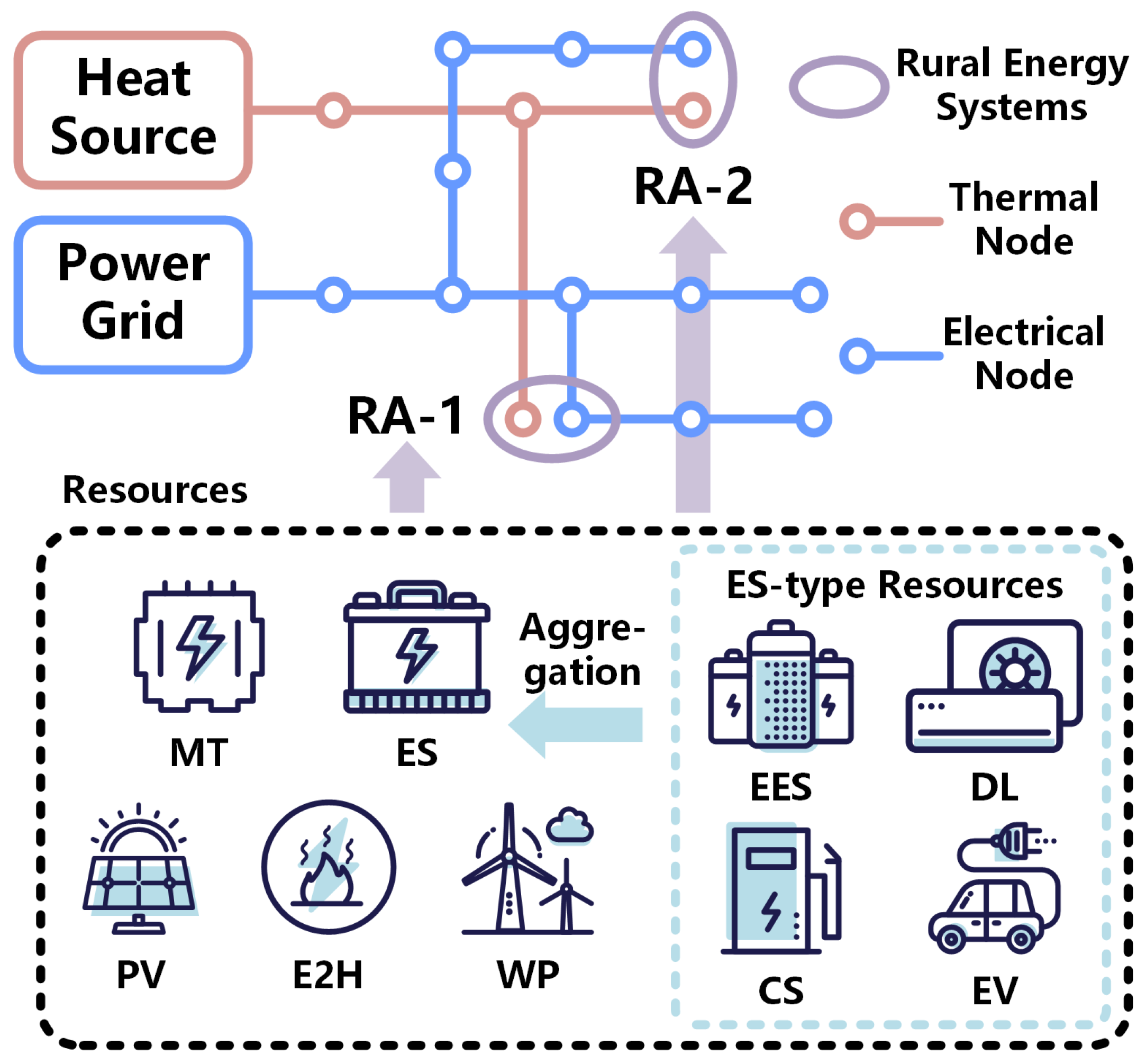
The proposed hierarchical coordinated optimization framework for RDES is illustrated in Figure 1. This framework integrates electrical and thermal networks in rural areas, enabling coordinated energy management across multiple types of DERs. The system includes electrical and thermal nodes, respectively connected to the power grid and a centralized heat source, facilitating bi-directional energy flows and multi-energy coupling.

In this RDES, multiple rural integrated energy areas (abbreviated as RAs in the figure) are deployed. Each RA incorporates various DERs, such as microturbines (MT), PV, electric-to-heat devices (E2H), wind power (WP), and general ES. A specific subset of these, referred to as ES-type resources, includes electrical energy storage (EES), EV, charging station (CS), and demand-side load (DL). These resources provide enhanced flexibility and can be aggregated for coordinated scheduling. Each RA (e.g., RA-1, RA-2) is responsible for managing local energy resources, aggregating their flexibility, and interacting with the upper-level system to achieve global optimization.

A two-level coordination mechanism is adopted in this RDES. The upper level, referred to as the distribution network Level, manages system-wide energy exchanges and performs global optimization. The lower level, termed the distribution transformer area level and coordinated by multiple RAs, focuses on local optimization by considering DER characteristics and responding to system-level signals. To enable distributed coordination between the two levels, the ADMM is employed. Electricity and heat prices are used as coupling variables to facilitate the exchange of information and ensure convergence between local and global objectives.

This hierarchical structure supports flexible, resilient, and efficient operation of rural multi-energy systems with high penetration of renewable and distributed technologies.

3. Optimization Model and Solution Approach

This paper hierarchically divides RDES into two coordination levels: the distribution transformer area level and the distribution network level. A dedicated model is established for each level to capture local operational flexibility and system-level constraints. At the lower level, ES-type resources—including EES, CS, EV, and DL—are aggregated to enhance controllability and provide unified flexibility services. A distributed optimization framework based on the ADMM is adopted to solve the multi-energy power flow and scheduling problem across the two levels, enabling coordinated decision-making while preserving the privacy and autonomy of local systems.

3.1. Aggregation Model of ES-Type Resources

To enhance system flexibility and simplify upper-level coordination, ES-type resources are aggregated at the RA level into a unified flexibility model. These ES-type resources include EES, EV, CS, and DL. Each of these components exhibits ES or load shifting characteristics and can be controlled in a dispatchable manner.

For ES-type resources, both power boundary constraints and energy boundary constraints are considered. The ES-type resources are formulated as follows:

$$\begin{array}{c}-{\underline{P}}_{i,k}^{\mathrm{ES}}\le P_{i,k,t}^{\mathrm{ES}}\le {\overline{P}}_{i,k}^{\mathrm{ES}}\end{array}$$

(1a)

$$\begin{array}{c}{E}_{i,k,t}^{\mathrm{ES}}={\theta }_{i,k}{E}_{i,k,t-1}^{\mathrm{ES}}+P_{i,k,t}^{\mathrm{ES}}\Delta t\end{array}$$

(1b)

$$\begin{array}{c}-{\underline{E}}_{i,k}^{\mathrm{ES}}\le E_{i,k,t}^{\mathrm{ES}}\le {\overline{E}}_{i,k}^{\mathrm{ES}}\end{array}$$

(1c)

where $P_{i,k,t}^{\mathrm{ES}}$ represents the output power of ES-type resource k in area i at time t, ${\overline{P}}_{i,k}^{\mathrm{ES}}$/$(-{\underline{P}}_{i,k}^{\mathrm{ES}})$ represents the maximum/minimum active power output of ES-type resource k in area i, $E_{i,k,t}^{\mathrm{ES}}$ represents the residual energy of ES-type resource k in area i at time t, ${\theta }_{i,k}$ represents the dissipation rate of ES-type resource k in area i, $\Delta t$ represents the time interval, and ${\overline{E}}_{i,k}^{\mathrm{ES}}$/$(-{\underline{E}}_{i,k}^{\mathrm{ES}})$ represents the upper/lower bound of the storage residual energy of ES-type resource k in area i.

It is worth noting that (1c) represents the power boundary constraint, where both the lower and upper bounds are positive values. During the inner approximation aggregation process, boundary shrinkage may occur. In actual computation, this is typically implemented by multiplying a scaling factor less than 1, which can result in the transformed lower bound being greater than the original one. To eliminate this issue, a further transformation of the constraint is required, as detailed below:

$$\begin{array}{c}{E}_{i,k,t}^{\mathrm{ES}}-{\tilde{E}}_{i,k}^{\mathrm{ES}}={\theta }_{i,k}{E}_{i,k,t-1}^{\mathrm{ES}}+P_{i,k,t}^{\mathrm{ES}}\Delta t-{\tilde{E}}_{i,k}^{\mathrm{ES}}\end{array}$$

(2a)

$$\begin{array}{c}-{\underline{E}}_{i,k}^{\mathrm{ES}}-{\tilde{E}}_{i,k}^{\mathrm{ES}}\le E_{i,k,t}^{\mathrm{ES}}-{\tilde{E}}_{i,k}^{\mathrm{ES}}\le {\overline{E}}_{i,k}^{\mathrm{ES}}-{\tilde{E}}_{i,k}^{\mathrm{ES}}\end{array}$$

(2b)

where ${\tilde{E}}_{i,k}^{\mathrm{ES}}=({\overline{E}}_{i,k}^{\mathrm{ES}}-{\underline{E}}_{i,k}^{\mathrm{ES}})/2$. Based on this, (1) can be reformulated as

$$\begin{array}{c}-{\underline{P}}_{i,k}^{\mathrm{ES}}\le P_{i,k,t}^{\mathrm{ES}}\le {\overline{P}}_{i,k}^{\mathrm{ES}}\end{array}$$

(3a)

$$\begin{array}{c}{E}_{i,k,t}^{*\mathrm{ES}}={\theta }_{i,k}{E}_{i,k,t-1}^{*\mathrm{ES}}+P_{i,k,t}^{\mathrm{ES}}\Delta t\end{array}$$

(3b)

$$\begin{array}{c}-{\underline{E}}_{i,k}^{*\mathrm{ES}}\le E_{i,k,t}^{*\mathrm{ES}}\le {\overline{E}}_{i,k}^{*\mathrm{ES}}\end{array}$$

(3c)

where $E_{i,k,t}^{*\mathrm{ES}}=E_{i,k,t}^{\mathrm{ES}}-{\tilde{E}}_{i,k}^{\mathrm{ES}}$, ${\underline{E}}_{i,k}^{*\mathrm{ES}}={\underline{E}}_{i,k}^{\mathrm{ES}}+{\tilde{E}}_{i,k}^{\mathrm{ES}}$, ${\overline{E}}_{i,k}^{*\mathrm{ES}}={\overline{E}}_{i,k}^{\mathrm{ES}}-{\tilde{E}}_{i,k}^{\mathrm{ES}}$. It is also important to note that, as a result of (3a), the initial energy value is given by $E_{i,k,0}^{*\mathrm{ES}}=E_{i,k,0}^{\mathrm{ES}}-{\tilde{E}}_{i,k}^{\mathrm{ES}}/{\theta }_{i,k}$.

The above model can be rewritten in a compact form as

$${\mathit{F}}_{i,k}^{\mathrm{ES}}{\mathit{P}}_{i,k}^{\mathrm{ES}}\le {\mathit{H}}_{i,k}^{\mathrm{ES}}$$

(4)

where ${\mathit{P}}_{i,k}^{\mathrm{ES}}={\left[P_{i,k,t}^{\mathrm{ES}}{|}_{t=1,...,T}\right]}^{\mathsf{T}}$, T represents the total number of time horizons. ${\mathit{F}}_{i,k}^{\mathrm{ES}}$ and ${\mathit{H}}_{i,k}^{\mathrm{ES}}$ are the parameter matrices of ES-type resource k in area i, with their detailed structures given below:

$$\begin{array}{c}{\mathit{F}}_{i,k}^{\mathrm{ES}}=[{\mathit{I}}_T;-{\mathit{I}}_T;{\mathit{A}}_{i,k}^{-1}{\mathit{B}}_{i,k};-{\mathit{A}}_{i,k}^{-1}{\mathit{B}}_{i,k}]\end{array}$$

(5a)

$$\begin{array}{c}{\mathit{H}}_{i,k}^{\mathrm{ES}}=[{\overline{\mathit{P}}}_{i,k}^{\mathrm{ES}};{\underline{\mathit{P}}}_{i,k}^{\mathrm{ES}};{\overline{\mathit{E}}}_{i,k}^{*\mathrm{ES}}-{\mathit{A}}_{i,k}^{-1}{\mathit{C}}_{i,k};{\underline{\mathit{E}}}_{i,k}^{*\mathrm{ES}}+{\mathit{A}}_{i,k}^{-1}{\mathit{C}}_{i,k}]\end{array}$$

(5b)

where ${\mathit{I}}_T$ denotes the T-dimensional identity matrix; ${\mathit{A}}_{i,k}={\mathit{I}}_T+diag(-{\theta }_{i,k};-1)$ is a lower bidiagonal matrix; ${\mathit{B}}_{i,k}=\Delta t{\mathit{I}}_T$; ${\mathit{C}}_{i,k}={[{\theta }_{i,k}{E}_{i,k,0}^{*\mathrm{ES}},0,\dots ,0]}^{\mathsf{T}}$; ${\overline{\mathit{P}}}_{i,k}^{\mathrm{ES}}={\overline{P}}_{i,k}^{\mathrm{ES}}{\mathbf{1}}_T$, in which ${\mathbf{1}}_T$ is the T-dimensional column vector of all ones; ${\underline{\mathit{P}}}_{i,k}^{\mathrm{ES}}={\underline{P}}_{i,k}^{\mathrm{ES}}{\mathbf{1}}_T$; ${\overline{\mathit{E}}}_{i,k}^{*\mathrm{ES}}={\overline{E}}_{i,k}^{*\mathrm{ES}}{\mathbf{1}}_T$; ${\underline{\mathit{E}}}_{i,k}^{*\mathrm{ES}}={\underline{E}}_{i,k}^{*\mathrm{ES}}{\mathbf{1}}_T$.

Based on the modified ES-type resource model described above, and following the maximum inner approximation aggregation method based on the Minkowski sum as adopted in [25], the aggregated ES k in area i $\left({\mathbb{B}}_{i,k}^A\right)$ can be approximated by a virtual ES $\left({\mathbb{B}}_i^0\right)$, which is constructed based on the average storage parameters within the area, i.e., ${\mathbb{B}}_{i,k}^A:={\beta }_{i,k}{\mathbb{B}}_i^0+{\mathit{t}}_{i,k}$. In this formulation, ${\beta }_{i,k}$ and ${\mathit{t}}_{i,k}$ represent the scaling and translation coefficients, respectively. These translation coefficients can be obtained by solving the following optimization problem:

$$\begin{array}{cccc}\hfill \underset{{\alpha }_{i,k},{\chi }_{i,k},{\mathit{G}}_{i,k}}{min}& {\alpha }_{i,k}\hfill & & \end{array}$$

(6a)

$$\begin{array}{cc}\hfill \mathrm{s}.\mathrm{t}.& {\mathit{G}}_{i,k}{\mathit{F}}_i^0={\mathit{F}}_{i,k}^{\mathrm{ES}},{\mathit{G}}_{i,k}\ge 0,\hfill \end{array}$$

(6b)

$$\begin{array}{cc}\hfill & {\mathit{G}}_{i,k}{\mathit{H}}_i^0\le {\alpha }_{i,k}{\mathit{H}}_{i,k}^{\mathrm{ES}}+{\chi }_{i,k}{\mathit{F}}_{i,k}^{\mathrm{ES}},{\alpha }_{i,k}\ge 0.\hfill \end{array}$$

(6c)

where ${\alpha }_{i,k}=1/{\beta }_{i,k}$, ${\chi }_{i,k}=-{\mathit{t}}_{i,k}/{\beta }_{i,k}$, ${\mathit{G}}_{i,k}$ is a auxiliary matrix variable. ${\mathit{F}}_i^0$ and ${\mathit{H}}_i^0$ are the parameter matrices of ${\mathbb{B}}_i^0$, which are calculated as follows:

$$\begin{array}{c}{\mathit{F}}_i^0=\sum _{k\in {\Psi }_i}{\mathit{F}}_{i,k}^{\mathrm{ES}}/N_i^{\mathrm{ES}}\end{array}$$

(7a)

$$\begin{array}{c}{\mathit{H}}_i^0=\sum _{k\in {\Psi }_i}{\mathit{H}}_{i,k}^{\mathrm{ES}}/N_i^{\mathrm{ES}}\end{array}$$

(7b)

where ${\Psi }_i$ represents the set of ES-type resources within area i, $N_i^{\mathrm{ES}}$ represents the number of ES-type resources in the area i.

The aggregated ES constraints for the rural integrated energy area i are formulated as follows:

$$\begin{array}{c}-{\underline{\mathit{P}}}_i^{\mathrm{ESA}}\left(t\right)\le P_{i,t}^{\mathrm{ESA}}\le {\overline{\mathit{P}}}_i^{\mathrm{ESA}}\left(t\right)\end{array}$$

(8a)

$$\begin{array}{c}{E}_{i,t}^{\mathrm{ESA}}={\theta }_i^{\mathrm{ESA}}{E}_{i,t-1}^{\mathrm{ESA}}+P_{i,t}^{\mathrm{ESA}}\Delta t\end{array}$$

(8b)

$$\begin{array}{c}-{\underline{\mathit{E}}}_i^{\mathrm{ESA}}\left(t\right)\le E_{i,t}^{\mathrm{ESA}}\le {\overline{\mathit{E}}}_i^{\mathrm{ESA}}\left(t\right)\end{array}$$

(8c)

where $P_{i,t}^{\mathrm{ESA}}$ represents the output power of aggregated ES in area i at time t, ${\overline{\mathit{P}}}_i^{\mathrm{ESA}}$/$(-{\underline{\mathit{P}}}_i^{\mathrm{ESA}})$ represents the maximum/minimum energy storage active power output of aggregated ES in area i, $E_{i,t}^{\mathrm{ESA}}$ represents the residual energy of energy storage of aggregated ES in area i at time t, ${\theta }_i^{\mathrm{ESA}}$ represents the dissipation rate of aggregated ES in area i, ${\overline{\mathit{E}}}_i^{\mathrm{ESA}}$/$(-{\underline{\mathit{E}}}_i^{\mathrm{ESA}})$ represents the upper/lower bound of the storage residual energy of aggregated ES in area i. The above parameters is given by

$$\begin{array}{c}{\underline{\mathit{P}}}_i^{\mathrm{ESA}}={\beta }_i{\underline{\mathit{P}}}_i^0-{\mathit{t}}_i\end{array}$$

(9a)

$$\begin{array}{c}{\overline{\mathit{P}}}_i^{\mathrm{ESA}}={\beta }_i{\overline{\mathit{P}}}_i^0+{\mathit{t}}_i\end{array}$$

(9b)

$$\begin{array}{c}{\underline{\mathit{E}}}_i^{\mathrm{ESA}}={\beta }_i{\underline{\mathit{E}}}_i^0-{\left({\mathit{A}}_i^0\right)}^{-1}{\mathit{B}}_i^0{\mathit{t}}_i+\sum _{k\in {\Psi }_i}{\tilde{E}}_{i,k}^{\mathrm{ES}}\end{array}$$

(9c)

$$\begin{array}{c}{\overline{\mathit{E}}}_i^{\mathrm{ESA}}={\beta }_i{\overline{\mathit{E}}}_i^0+{\left({\mathit{A}}_i^0\right)}^{-1}{\mathit{B}}_i^0{\mathit{t}}_i+\sum _{k\in {\Psi }_i}{\tilde{E}}_{i,k}^{\mathrm{ES}}\end{array}$$

(9d)

where ${\beta }_i={\sum }_{k\in {\Psi }_i}{\beta }_{i,k}$, ${\mathit{t}}_i={\sum }_{k\in {\Psi }_i}{\mathit{t}}_{i,k}$. ${\underline{\mathit{P}}}_i^0$, ${\overline{\mathit{P}}}_i^0$, ${\underline{\mathit{E}}}_i^0$ and ${\overline{\mathit{E}}}_i^0$ are parameter column vectors, whose entries represent the average values of the parameters corresponding to ES-type resources within area i. ${\mathit{A}}_i^0$, and ${\mathit{B}}_i^0$ are the parameter matrices of ${\mathbb{B}}_i^0$, with structures similar to ${\mathit{A}}_{i,k}$ and ${\mathit{B}}_{i,k}$.

3.2. Distribution Transformer Area-Level Model

In the distribution transformer area-level model of rural energy systems, it is essential to satisfy both the load demands of various energy consumers within the area and the grid integration requirements of distributed energy resources. This paper considers the electric, thermal, and cooling load demands in rural transformer areas, as well as the grid compatibility constraints for PV, WP, ES, and MT. An optimization model for rural energy systems at the transformer area level is developed, with the objective of minimizing the total energy procurement cost and operation maintenance costs. The objective function is formulated as follows:

$$\begin{array}{cc}\hfill min{C}_i^{\mathrm{AL}}& =\sum _{t\in T}\left(p_{e,t}{P}_{i,t}+p_{h,t}{H}_{i,t}\right)\Delta t\hfill \\ \hfill & +\sum _{t\in T}({\delta }_i^{\mathrm{PV}}{P}_{i,t}^{\mathrm{PV}}+{\delta }_i^{\mathrm{WP}}{P}_{i,t}^{\mathrm{WP}}+{\delta }_i^{\mathrm{MT}}{P}_{i,t}^{\mathrm{MT}}\hfill \\ \hfill & +{\delta }_i^{\mathrm{ESA}}\left|P_{i,t}^{\mathrm{ESA}}\right|+{\delta }_i^{\mathrm{E}2\mathrm{H}}{P}_{i,t}^{\mathrm{E}2\mathrm{H}}+\hfill \\ \hfill & {\delta }_i^{\mathrm{E}2\mathrm{L}}{P}_{i,t}^{\mathrm{E}2\mathrm{L}}+{\delta }_i^{\mathrm{H}2\mathrm{L}}{H}_{i,t}^{\mathrm{H}2\mathrm{L}})\Delta t\hfill \end{array}$$

(10)

where $C_i^{\mathrm{AL}}$ represents the distribution transformer area-level (AL) operating cost of area i, $P_{i,t}$, and $H_{i,t}$, respectively, represent the purchased electrical energy and thermal energy of area i at time t, $p_{e,t}$ and $p_{h,t}$, respectively, denote the prices of purchased electrical energy and thermal energy at time t, ${\delta }_i^{*}$ represents the operation and maintenance costs of Equipment ∗ of area i, $P_{i,t}^{*}$ and $H_{i,t}^{*}$, respectively, represent the output electrical energy and thermal energy of Equipment * of area i at time t. Here, E2H refers to electric heating equipment, E2L refers to electric cooling equipment, and H2L refers to absorption cooling equipment. Constraints include equipment operation constraints and power balance constraints, as detailed below:

3.2.1. Photovoltaic Model

$$0\le P_{i,t}^{\mathrm{PV}}\le {\overline{P}}_i^{\mathrm{PV}}$$

(11)

where ${\overline{P}}_i^{\mathrm{PV}}$ represents the maximum PV active power output of area i.

3.2.2. Wind Power Model

$$0\le P_{i,t}^{\mathrm{WP}}\le {\overline{P}}_i^{\mathrm{WP}}$$

(12)

where ${\overline{P}}_i^{\mathrm{WP}}$ represents the maximum wind power active power output of area i.

3.2.3. Micro Gas Turbines Model

$$\begin{array}{c}0\le P_{i,t}^{\mathrm{MT}}\le {\overline{P}}_i^{\mathrm{MT}}\end{array}$$

(13a)

$$\begin{array}{c}-R_i^{\mathrm{MT}}\le P_{i,t}^{\mathrm{MT}}-P_{i,t-1}^{\mathrm{MT}}\le R_i^{\mathrm{MT}}\end{array}$$

(13b)

where ${\overline{P}}_i^{\mathrm{MT}}$ represents the maximum micro gas turbines’ active power output of area i, $R_i^{\mathrm{MT}}$ represents the maximum ramp rate of micro gas turbines of area i.

3.2.4. Energy Storage Aggregation Model

A complete derivation of this part of the model is presented in the earlier sections of the paper, detailed information can be found in (8) and (9).

$$\begin{array}{c}-{\underline{\mathit{P}}}_i^{\mathrm{ESA}}\left(t\right)\le P_{i,t}^{\mathrm{ESA}}\le {\overline{\mathit{P}}}_i^{\mathrm{ESA}}\left(t\right)\end{array}$$

(14a)

$$\begin{array}{c}{E}_{i,t}^{\mathrm{ESA}}={\theta }_i^{\mathrm{ESA}}{E}_{i,t-1}^{\mathrm{ESA}}+P_{i,t}^{\mathrm{ESA}}\Delta t\end{array}$$

(14b)

$$\begin{array}{c}-{\underline{\mathit{E}}}_i^{\mathrm{ESA}}\left(t\right)\le E_{i,t}^{\mathrm{ESA}}\le {\overline{\mathit{E}}}_i^{\mathrm{ESA}}\left(t\right)\end{array}$$

(14c)

3.2.5. Energy Conversion Equipment Model

$$\begin{array}{c}{H}_{i,t}^{\mathrm{E}2\mathrm{H}}={\lambda }_i^{\mathrm{E}2\mathrm{H}}{P}_{i,t}^{\mathrm{E}2\mathrm{H}}\end{array}$$

(15a)

$$\begin{array}{c}0\le H_{i,t}^{\mathrm{E}2\mathrm{H}}\le {\overline{H}}_i^{\mathrm{E}2\mathrm{H}}\end{array}$$

(15b)

$$\begin{array}{c}{L}_{i,t}^{\mathrm{E}2\mathrm{L}}={\lambda }_i^{\mathrm{E}2\mathrm{L}}{P}_{i,t}^{\mathrm{E}2\mathrm{L}}\end{array}$$

(15c)

$$\begin{array}{c}0\le L_{i,t}^{\mathrm{E}2\mathrm{L}}\le {\overline{L}}_i^{\mathrm{E}2\mathrm{L}}\end{array}$$

(15d)

$$\begin{array}{c}{L}_{i,t}^{\mathrm{H}2\mathrm{L}}={\lambda }_i^{\mathrm{H}2\mathrm{L}}{H}_{i,t}^{\mathrm{H}2\mathrm{L}}\end{array}$$

(15e)

$$\begin{array}{c}0\le L_{i,t}^{\mathrm{H}2\mathrm{L}}\le {\overline{L}}_i^{\mathrm{H}2\mathrm{L}}\end{array}$$

(15f)

where $H_{i,t}^{\mathrm{E}2\mathrm{H}}$ represents the E2H’s thermal energy output of area i at time t, $L_{i,t}^{\mathrm{E}2\mathrm{L}}$ represents the E2L’s cooling power output of area i at time t, $L_{i,t}^{\mathrm{H}2\mathrm{L}}$ represents the H2L’s cooling power output of area i at time t, ${\overline{H}}_i^{\mathrm{E}2\mathrm{H}}$ represents the maximum E2H’s thermal energy output of area i, ${\overline{L}}_i^{\mathrm{E}2\mathrm{L}}$ represents the maximum E2L’s cooling power output of area i, ${\overline{L}}_i^{\mathrm{H}2\mathrm{L}}$ the maximum H2L’s cooling power output of area i. ${\lambda }_i^{\mathrm{E}2\mathrm{H}}$, ${\lambda }_i^{\mathrm{E}2\mathrm{L}}$, and ${\lambda }_i^{\mathrm{H}2\mathrm{L}}$, respectively, represents the conversion coefficient of the corresponding equipment. Three values are set to 4.5, 4, and 3 in this paper.

3.2.6. Energy Balance Relationship

$$\begin{array}{c}{P}_{i,t}^{\mathrm{PV}}+P_{i,t}^{\mathrm{WP}}+P_{i,t}^{\mathrm{MT}}+P_{i,t}^{\mathrm{ESA}}+P_{i,t}=P_{i,t}^{\mathrm{E}2\mathrm{H}}+P_{i,t}^{\mathrm{E}2\mathrm{L}}+P_{i,t}^{\mathrm{LD}}\end{array}$$

(16a)

$$\begin{array}{c}{H}_{i,t}^{\mathrm{E}2\mathrm{H}}+H_{i,t}=H_{i,t}^{\mathrm{H}2\mathrm{L}}+H_{i,t}^{\mathrm{LD}}\end{array}$$

(16b)

$$\begin{array}{c}{L}_{i,t}^{\mathrm{E}2\mathrm{L}}+L_{i,t}^{\mathrm{H}2\mathrm{L}}=L_{i,t}^{\mathrm{LD}}\end{array}$$

(16c)

where $P_{i,t}^{\mathrm{LD}}$ represents the electrical load of area i at time t, $H_{i,t}^{\mathrm{LD}}$ represents the thermal load of area i at time t, and $L_{i,t}^{\mathrm{LD}}$ represents the cooling load of area i at time t.

3.3. Distribution Network-Level Model

The operational cost of the rural distributed system’s distribution network-level model includes two parts: the cost of purchasing electricity from the main grid and the cost of selling electricity to the transformer area-level model. When the result is negative, it indicates that the distribution network level is profitable; when the result is positive, it signifies a loss at the distribution network level. The specific objective function is as follows:

$$\begin{array}{c}\hfill min{C}^{\mathrm{NL}}=\sum _{t\in T}\left(p_{e,t}^G{P}_t^G+p_{h,t}^G{H}_t^G\right)\Delta t-\sum _{t\in T}\sum _{i\in \Omega }\left(p_{e,t}{P}_{i,t}+p_{h,t}{H}_{i,t}\right)\Delta t\end{array}$$

(17)

where $C^{\mathrm{NL}}$ represents the distribution network-level (NL) operating cost, $P_{i,t}^G$ and $H_{i,t}^G$, respectively, represent the quantities of energy purchased from the superior power grid and the superior heat source at time t, $p_{e,t}$ and $p_{h,t}$ respectively denote the energy procurement costs from the superior power grid and the superior heat source at time t, and $\Omega$ represents the set of area-level models. The constraints primarily include power grid constraints and thermal network constraints, which are detailed as follows:

3.3.1. Power Grid Model

$$\begin{array}{c}{P}_{t,k}^D=\sum _{j\in {\mathbf{C}}_k}{P}_{t,j}^D+p_{t,k}^D\end{array}$$

(18a)

$$\begin{array}{c}{p}_{t,k}^D=p_{t,k}^{load}+P_{i,t}\end{array}$$

(18b)

$$\begin{array}{c}{Q}_{t,k}^D=\sum _{j\in {\mathbf{C}}_k}{Q}_{t,j}^D+q_{t,k}^D\end{array}$$

(18c)

$$\begin{array}{c}{q}_{t,k}^D=q_{t,k}^{load}\end{array}$$

(18d)

$$\begin{array}{c}{U}_{t,k}=U_{{\pi }_k}-r_k{P}_{t,k}^D-x_k{Q}_{t,k}^D,k\in \mathcal{N}/1\end{array}$$

(18e)

$$\begin{array}{c}-\overline{P^D}\le P_{t,k}^D\le \overline{P^D}\end{array}$$

(18f)

$$\begin{array}{c}-\overline{Q^D}\le Q_{t,k}^D\le \overline{Q^D}\end{array}$$

(18g)

$$\begin{array}{c}\underline{U}\le U_{t,k}\le \overline{U}\end{array}$$

(18h)

where $P_{t,k}^D$ and $Q_{t,k}^D$, respectively, represent the distribution network active and reactive power of node k’s line at time t. ${\mathbf{C}}_k$ denotes the set of children nodes of node k. $p_{t,k}^D$ and $q_{t,k}^D$, respectively, represent the distribution network-injected active and reactive power of the node k at time t. $p_{t,k}^{load}$ and $q_{t,k}^{load}$ represent the distribution network active and reactive power of the load at node k at time t, respectively. $U_{t,k}$ is the distribution network voltage at node k at time t. ${\pi }_k$ represent the father node of node k. $r_k$ and $x_k$ respectively denote the resistance and reactance of line k. $\mathcal{N}$ represents the set of all nodes. $\overline{P^D}$ and $\overline{Q^D}$ represent the distribution network upper limits of the active and reactive power transmission capacities of the line, respectively. $\overline{U}$ and $\underline{U}$ are the upper and lower bounds of the node voltage, respectively.

3.3.2. Thermal Network Model

$$\begin{array}{c}{H}_{t,k}^D=\sum _{j\in {\mathit{R}}_k}{H}_{t,j}^D+h_{t,k}^D\end{array}$$

(19a)

$$\begin{array}{c}{h}_{t,k}^D=h_{t,k}^{load}+H_{i,t}\end{array}$$

(19b)

$$\begin{array}{c}-\overline{H^D}\le H_{t,k}^D\le \overline{H^D}\end{array}$$

(19c)

where $H_{t,k}^D$ represents the thermal network power of node k’s line at time t. ${\mathit{R}}_k$ denotes the set of thermal network children nodes of node k. $h_{t,k}^D$ represents the thermal network injected power of the node k at time t. $h_{t,k}^{load}$ represents the thermal network power of the thermal load at node k at time t. $\overline{H^D}$ represents the thermal network upper limits of the thermal power transmission capacities of the line.

3.4. Distributed Coordination via ADMM

Leveraging the transformer area-level model and the distribution network-level optimal operation model established earlier, this section employs the ADMM to achieve distributed autonomy and decentralized optimization among all participating entities.

The upper and lower layer optimization models are connected through variables $P_{i,t}$ and $H_{i,t}$. Based on this relationship, the original objective function is augmented with Lagrangian relaxation, resulting in the augmented Lagrangian objective function for the upper- and lower-layer optimization problems.

In the lower-layer model, each transformer area-level model is solved individually, with the specific augmented Lagrangian function as follows:

$$\begin{array}{cc}\hfill min{\mathit{L}}_i^{\mathrm{AL}}({\mathit{X}}^{\mathrm{NL}},{\mathit{X}}^{\mathrm{AL}},\xi )& =C_i^{\mathrm{AL}}+\sum _{t\in T}{\xi }_{i,t}^e\left(P_{i,t}^{\mathrm{NL}}-P_{i,t}^{\mathrm{AL}}\right)+\sum _{t\in T}{\xi }_{i,t}^h\left(H_{i,t}^{\mathrm{NL}}-H_{i,t}^{\mathrm{AL}}\right)\hfill \\ \hfill & +\rho \sum _{t\in T}{\left(P_{i,t}^{\mathrm{NL}}-P_{i,t}^{\mathrm{AL}}\right)}^2+\rho \sum _{t\in T}{\left(H_{i,t}^{\mathrm{NL}}-H_{i,t}^{\mathrm{AL}}\right)}^2,\forall i\in \Omega \hfill \end{array}$$

(20)

where ${\mathit{X}}^{\mathrm{NL}}$ represents the decision variables of the upper-layer distribution network-level model, which include $P_{i,t}^{\mathrm{NL}}$ and $H_{i,t}^{\mathrm{NL}}$. ${\mathit{X}}^{\mathrm{AL}}$ represents the decision variables of the lower-layer transformer area-level model, which include $P_{i,t}^{\mathrm{AL}}$ and $H_{i,t}^{\mathrm{AL}}$. $\xi$ represents the Lagrange multipliers, which include ${\xi }_{i,t}^e$ and ${\xi }_{i,t}^h$. $\rho$ is the penalty factor, which is set to 1 in this paper.

The augmented Lagrangian objective function for the upper-layer distribution network-level model is as follows:

$$\begin{array}{cc}\hfill min{\mathit{L}}^{\mathrm{NL}}({\mathit{X}}^{\mathrm{NL}},{\mathit{X}}^{\mathrm{AL}},\xi )& =C^{\mathrm{NL}}+\sum _{t\in T}\sum _{i\in \Omega }{\xi }_{i,t}^e\left(P_{i,t}^{\mathrm{NL}}-P_{i,t}^{\mathrm{AL}}\right)+\sum _{t\in T}\sum _{i\in \Omega }{\xi }_{i,t}^h\left(H_{i,t}^{\mathrm{NL}}-H_{i,t}^{\mathrm{AL}}\right)\hfill \\ \hfill & +\rho \sum _{t\in T}\sum _{i\in \Omega }{\left(P_{i,t}^{\mathrm{NL}}-P_{i,t}^{\mathrm{AL}}\right)}^2+\rho \sum _{t\in T}\sum _{i\in \Omega }{\left(H_{i,t}^{\mathrm{NL}}-H_{i,t}^{\mathrm{AL}}\right)}^2\hfill \end{array}$$

(21)

The update formulas for the parameters and variables are as follows:

$${\mathit{X}}_{i,n+1}^{\mathrm{AL}}=argmin{\mathit{L}}_i^{\mathrm{AL}}({\mathit{X}}_n^{\mathrm{NL}},{\mathit{X}}_i^{\mathrm{AL}},{\xi }_n)$$

(22)

$${\mathit{X}}_{n+1}^{\mathrm{NL}}=argmin{\mathit{L}}^{\mathrm{NL}}({\mathit{X}}^{\mathrm{NL}},{\mathit{X}}_{n+1}^{\mathrm{AL}},{\xi }_n)$$

(23)

$${\xi }_{n+1}={\xi }_n+\rho ({\mathit{X}}_{n+1}^{\mathrm{NL}}-{\mathit{X}}_{n+1}^{\mathrm{AL}})$$

(24)

$${\parallel {\mathit{r}}_{n+1}\parallel }_2={\parallel {\mathit{X}}_{n+1}^{\mathrm{NL}}-{\mathit{X}}_{n+1}^{\mathrm{AL}}\parallel }_2$$

(25)

$${\parallel {\mathit{s}}_{n+1}\parallel }_2=\rho {\parallel {\mathit{X}}_{n+1}^{\mathrm{NL}}-{\mathit{X}}_n^{\mathrm{NL}}\parallel }_2$$

(26)

In the equations above, (22) represents the update formula for the decision variables of the lower-layer transformer area-level model, (23) represents the update formula for the decision variables of the upper-layer distribution network-level model, (24) represents the update formula for the Lagrangian multipliers, (25) represents the calculation formula for the primal residual, and (26) represents the calculation formula for the dual residual.

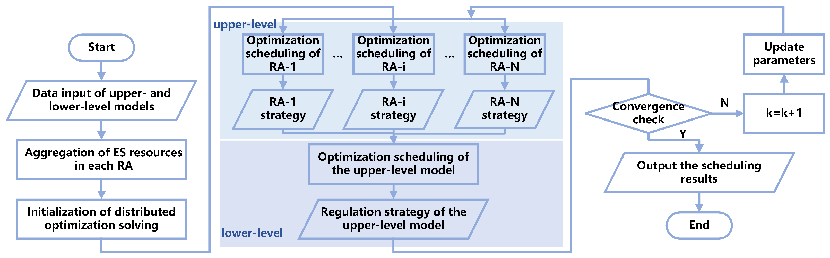
The specific solution process for the hierarchical collaborative optimization method of rural distributed energy systems based on the ADMM is as follows:

-

Step 1. Initialize the optimization parameters for both the upper- and lower-layer models, and set the iteration count to 1.

-

Step 2. Each transformer area-level model in the lower layer performs optimization based on Equation (22), and the resulting energy procurement scheme is fed back to the upper-layer distribution network model.

-

Step 3. The upper-layer distribution network-level model receives data from the lower-layer models and performs optimization based on Equation (23).

-

Step 4. The upper-layer distribution network-level model calculates the primal and dual residuals according to Equations (25) and (26), and determines whether they are less than the predefined thresholds.

-

Step 5. If the residuals are less than the predefined thresholds (it is set to ${10}^{-3}$ in this paper), the optimization results for each participating entity are output. Otherwise, the iteration count is incremented by one, the Lagrangian multipliers are updated, and the process returns to Step 2.

Based on the previous research, the hierarchical distributed control flowchart considering energy storage aggregation is shown in Figure 2.

4. Numerical Results

4.1. Simulation Setup

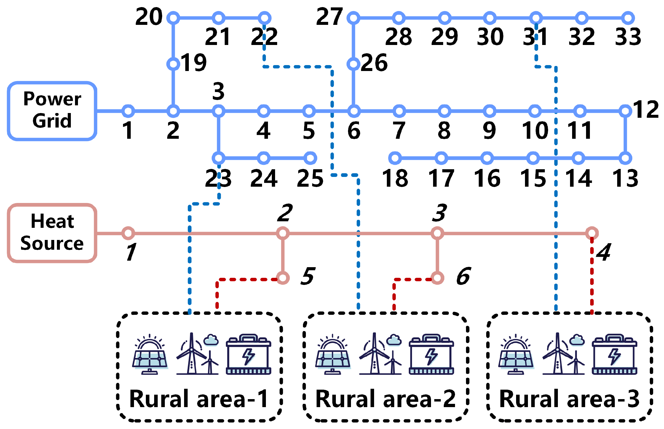
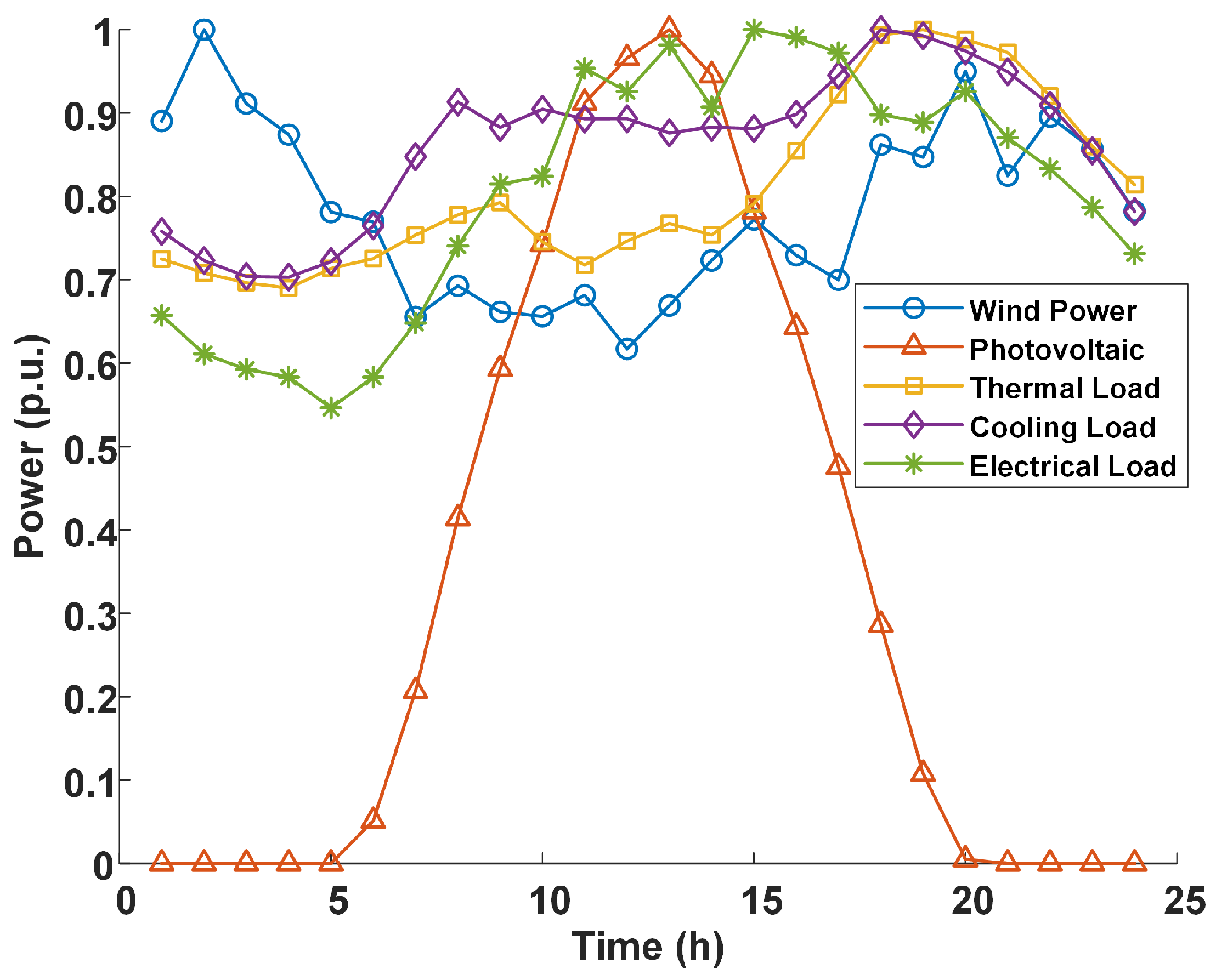
To validate the effectiveness and superiority of the proposed method, this paper constructs a test network for a RDES, which includes an IEEE-33 node distribution system and a 6-node thermal network, as illustrated in Figure 3. The test network encompasses three RAs, each containing five ES-type resources. The operational parameters of the equipment within each rural area are consistent, and the maximum predicted output of renewable energy sources such as wind and solar, as well as the cooling, heating, and electrical loads, are all uniform. The specific curves are shown in Figure 4. The installed capacity of the WP is 6.25 MW, the installed capacity of the PV is 4.7 MW, the installed capacity of the MT is 2.4 MW, the maximum output limit of the E2H is 6.25 MW, the maximum output limit of the E2L is 2.4 MW, and the maximum output limit of the H2L is 2.4 MW. The parameters of the ES-type resources are shown in

Table 1. The maximum power output limit ${\overline{P}}^{\mathrm{ES}}$ and energy capacity limit ${\overline{E}}^{\mathrm{ES}}$ of the ES-type resources.

${\overline{\mathit{P}}}^{\mathbf{ES}}/{\overline{\mathit{E}}}^{\mathbf{ES}}$ (MW/MWh)	DER-1	DER-2	DER-3	DER-4	DER-5
RA-1	0.5625/2.8125	0.5000/2.1875	0.6250/2.5000	0.3750/1.8750	0.5625/2.8125
RA-2	0.6250/3.1250	0.4375/1.8750	0.6250/3.1250	0.5000/2.5000	0.4375/1.8750
RA-3	0.4375/2.1875	0.4375/1.8750	0.7500/3.1250	0.5625/2.8125	0.5000/2.1875

.

The simulation is performed using MATLAB on a PC with an Intel Core i9 of 2.6 GHz and 16 GB memory. The problem is solved using a combination of YALMIP and CPLEX solvers.

4.2. Results and Discussion

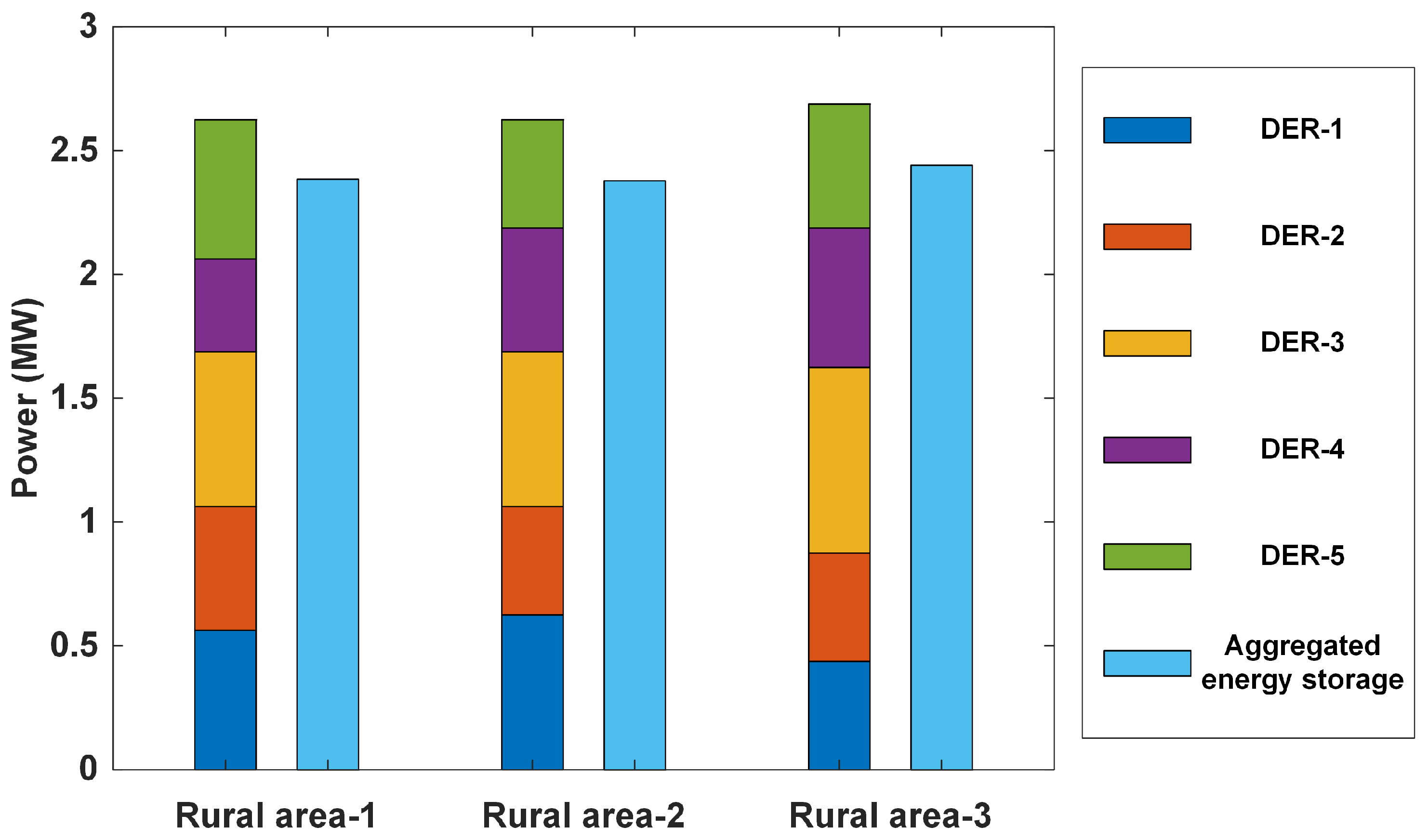
From the previous discussion, it can be seen that the aggregation method adopted in this paper is an inner approximation aggregation approach. To ensure the feasibility of resource aggregation and improve computational efficiency, this type of method cannot achieve 100% aggregation of resources. The theoretical maximum output values of ES-type resources before and after aggregation are given in

Table 2. The maximum output power of ES-type resources before and after aggregation.

Power (MW)	DER-1	DER-2	DER-3	DER-4	DER-5	Sum	ESA
RA-1	0.5625	0.5000	0.6250	0.3750	0.5625	2.6250	2.3845
RA-2	0.6250	0.4375	0.6250	0.5000	0.4375	2.6250	2.3783
RA-3	0.4375	0.4375	0.7500	0.5625	0.5000	2.6875	2.4412

. Figure 5 presents a comparison of the maximum output of ES-type resources before and after aggregation. By comparing the sum of the maximum outputs of the five individual ES-type resources before aggregation with that of the aggregated ES-type resource (ESA), the proposed aggregation method is able to keep this loss within 10%.

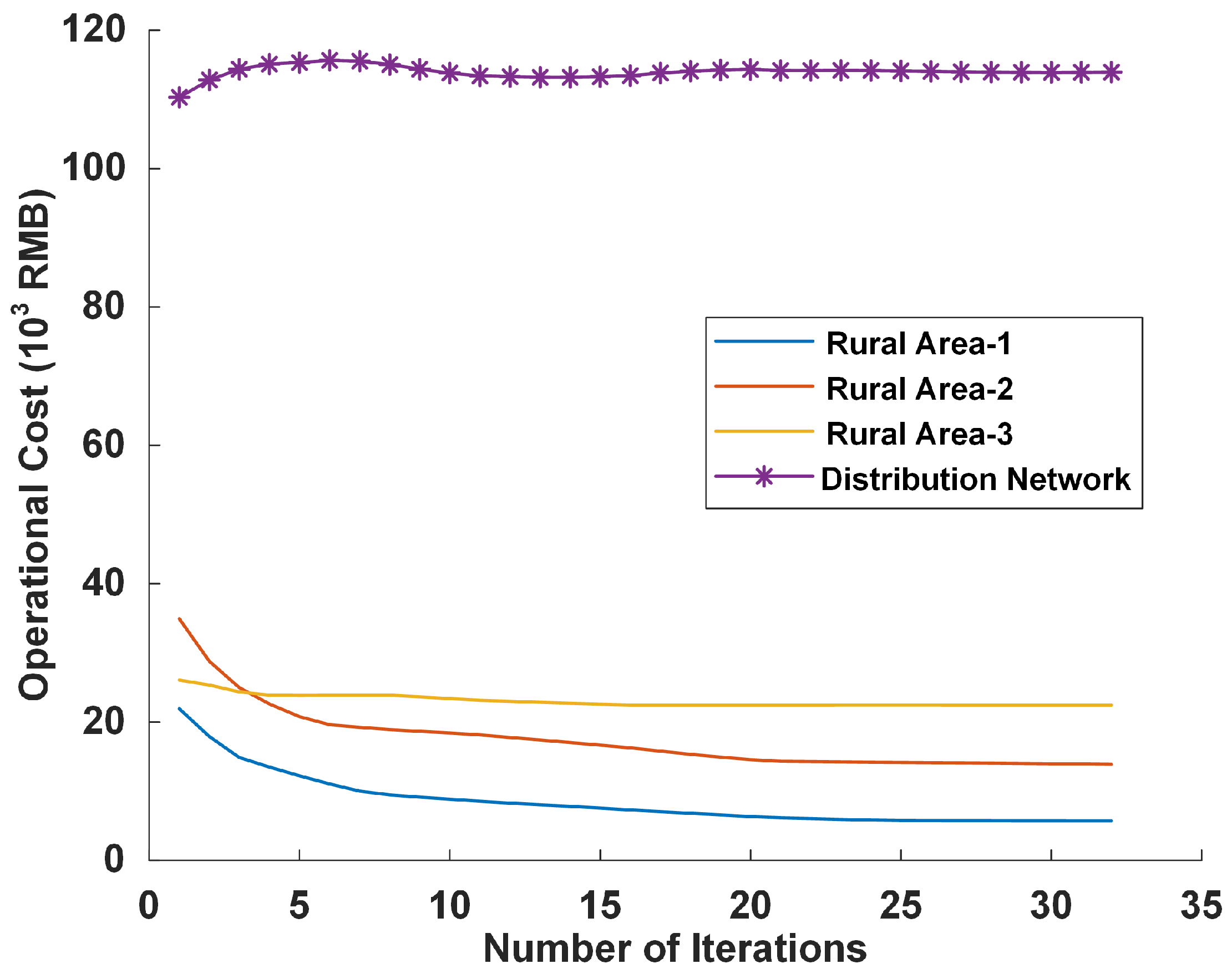
Figure 6 illustrates the changes in operational costs of each participating entity during the iteration process. As can be seen from Figure 6, during the collaborative iterative operation, the optimization decisions of both the upper and lower levels are influenced by each other, necessitating continuous adjustments to their respective scheduling strategies by each participating entity. At the beginning of the iterative optimization, due to the initial value settings, the upper and lower levels did not receive feedback information, resulting in drastic changes in the operational costs of each participating entity. As the iterative optimization progresses, the magnitude of strategy adjustments by each participating entity continuously decreases. After 33 iterations, the operational costs of each participating entity tend to stabilize. Finally, the operational cost of Rural Area-1 stabilizes at 5719 RMB, Rural Area-2 at 13,877 RMB, Rural Area-3 at 22,465 RMB, and the distribution network at 113,947 RMB. It is important to note that the distribution network not only supplies power to the three rural areas but also to other load nodes, resulting in higher costs. This demonstrates that the method proposed in this paper can achieve convergent and effective optimal scheduling results.

The method proposed in this paper is referred to as Method1, the centralized optimization considering energy storage aggregation is referred to as Method2, and the distributed optimization without considering energy storage aggregation is referred to as Method3. The solution results of the three methods are shown in

Table 3. Comparison of solution results under the three methods.

Method	RA-1 Cost (RMB)	RA-2 Cost (RMB)	RA-3 Cost (RMB)	NL Cost (RMB)	Total Cost (RMB)	Solving Time (s)
Method1	5719	13,877	22,465	113,947	156,008	94
Method2	5673	13,881	22,312	112,842	154,708	76
Method3	5723	13,899	22,997	116,021	158,640	583

. Although the total cost of Method1 is slightly higher than that of Method2, the difference is minimal. At the same time, Method1 retains the structural advantages of distributed optimization, enabling decentralized information processing and autonomous decision-making among multiple agents, making it more suitable for large-scale or privacy-constrained scenarios. In addition, the solving time of Method1 is only slightly longer than that of Method2 but much shorter than that of the distributed Method3 without considering energy storage aggregation. This indicates that Method1 maintains high computational efficiency while improving system economy through coordinated aggregation. Overall, Method1 fully leverages the advantages of distributed optimization in flexibility, scalability, and privacy protection, while keeping a total cost close to that of centralized optimization, demonstrating strong practical application potential.

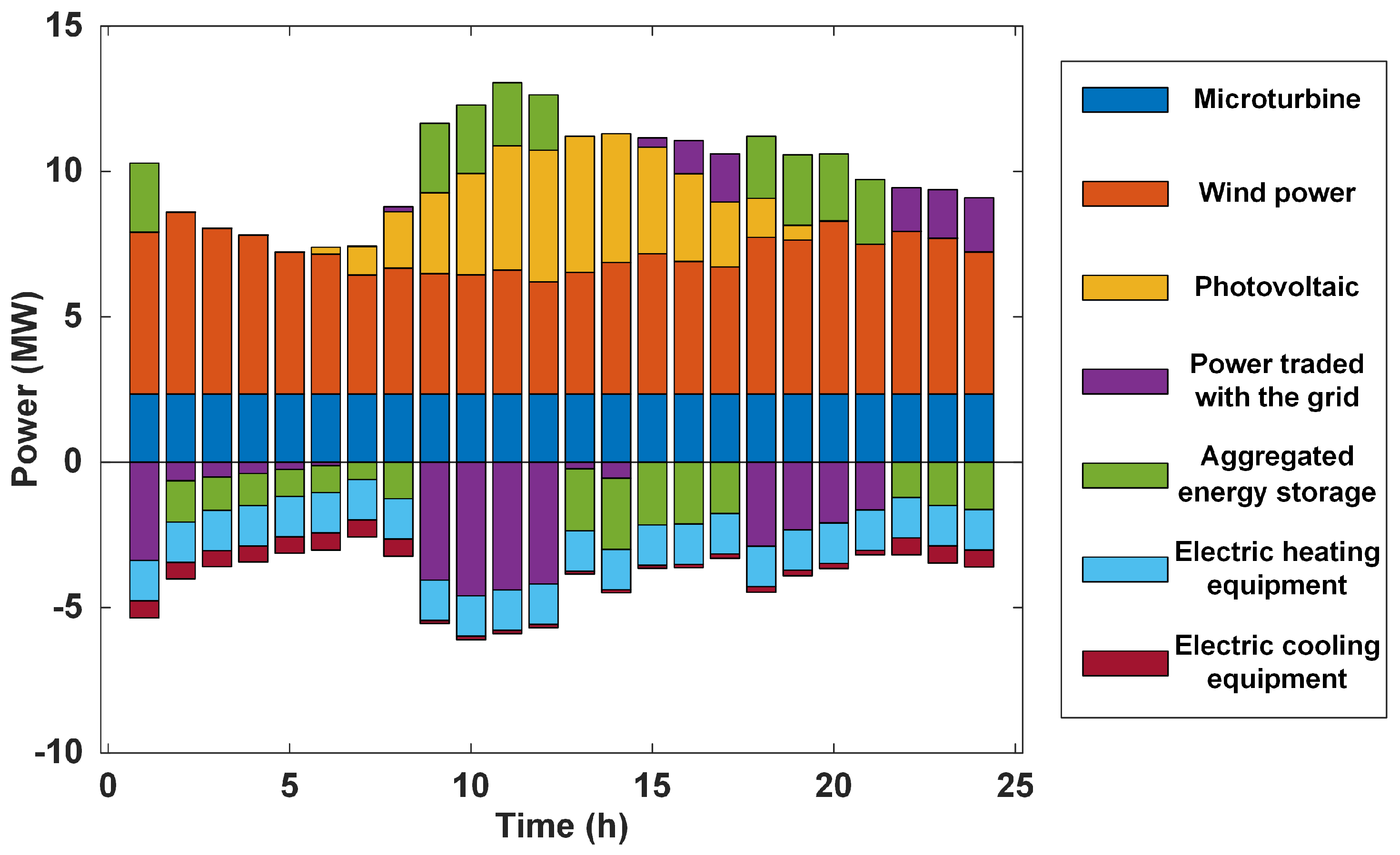
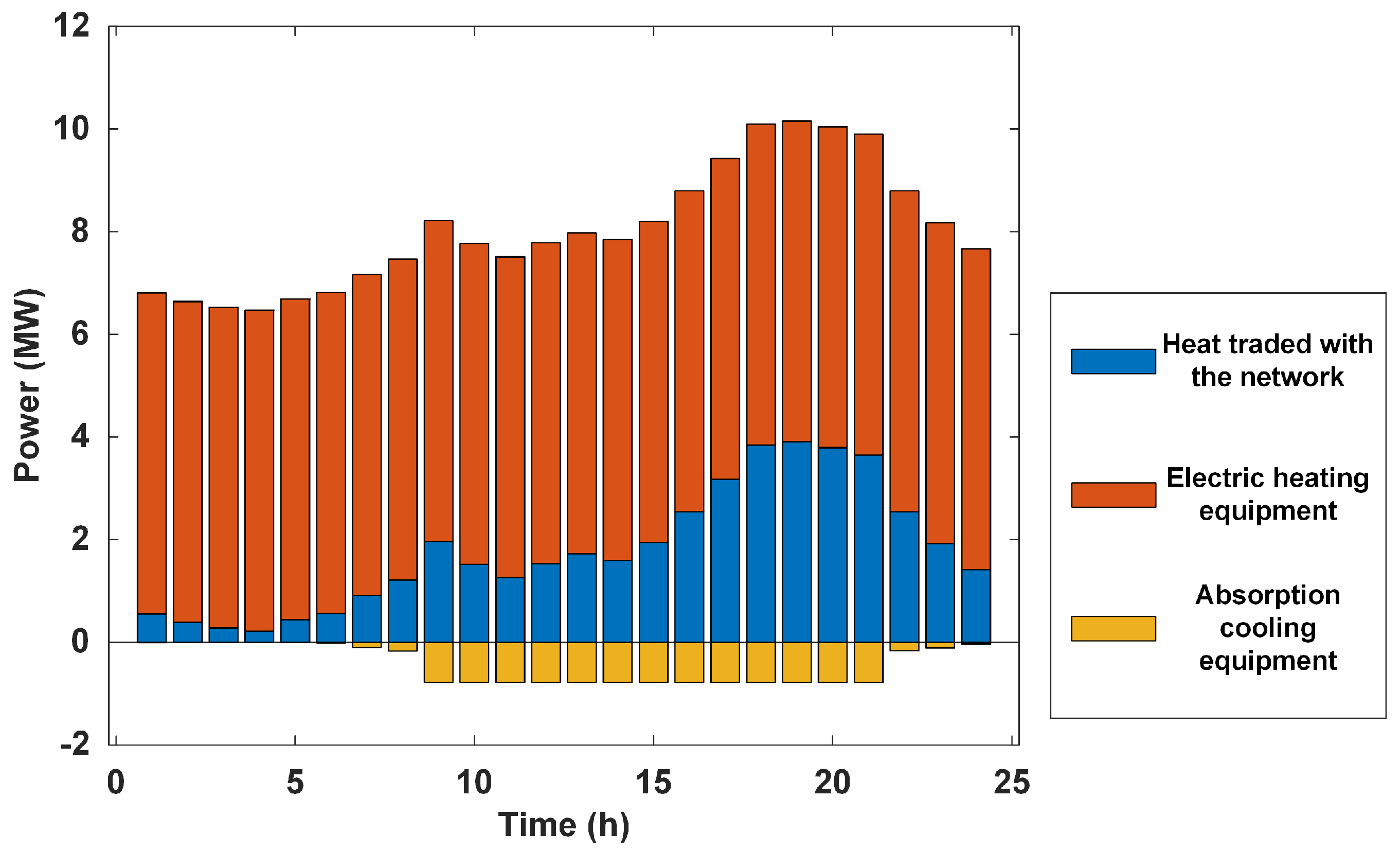
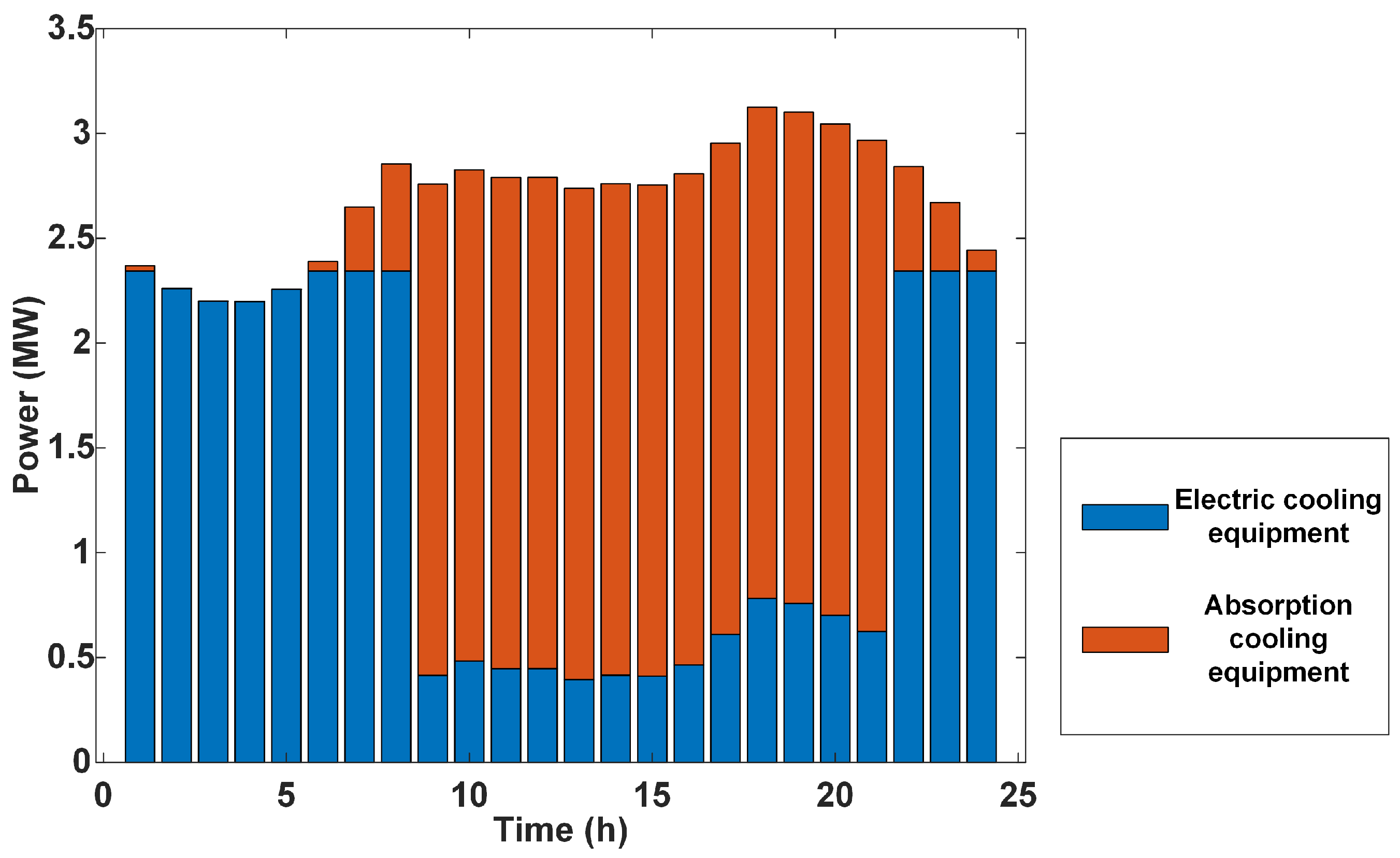
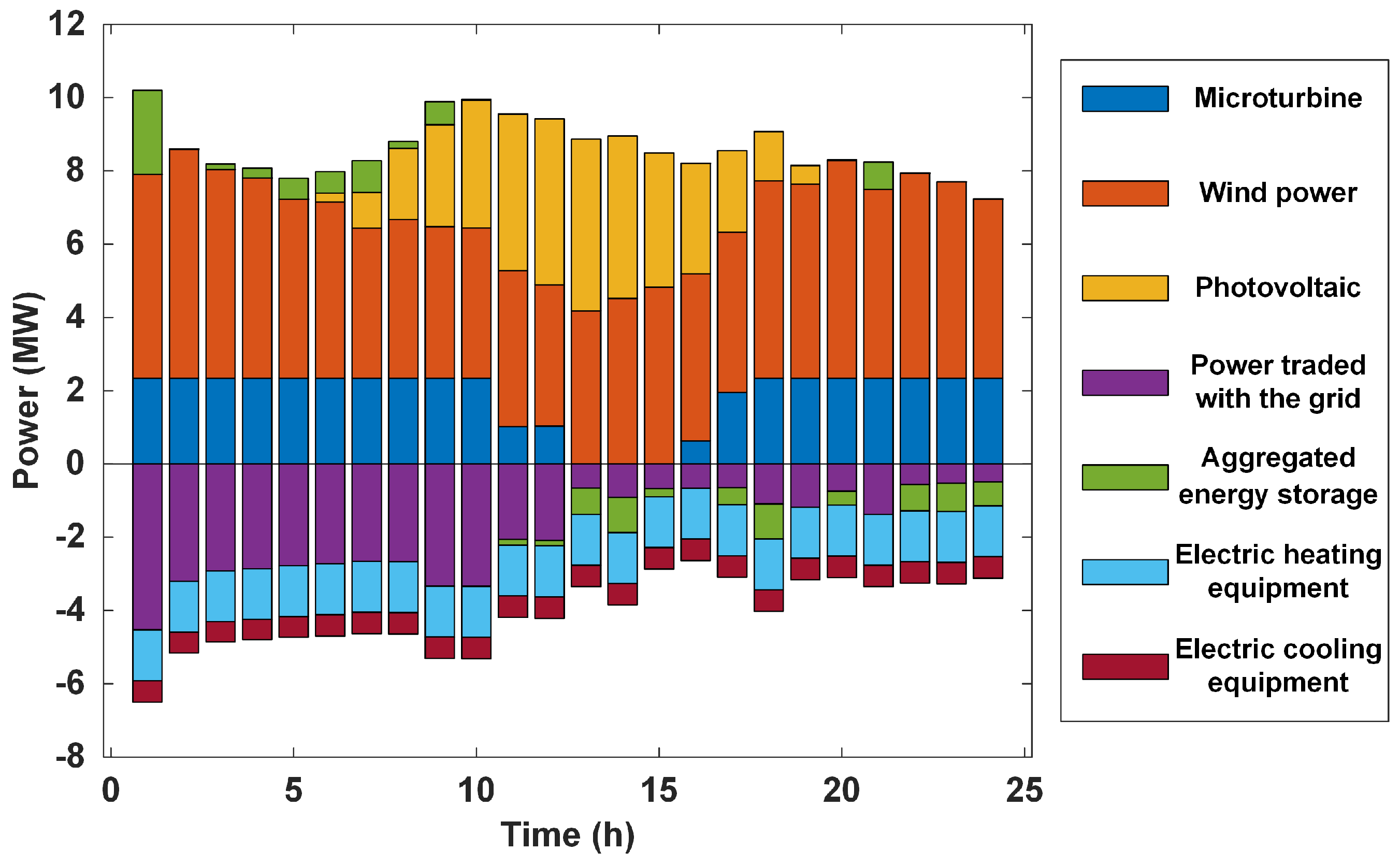
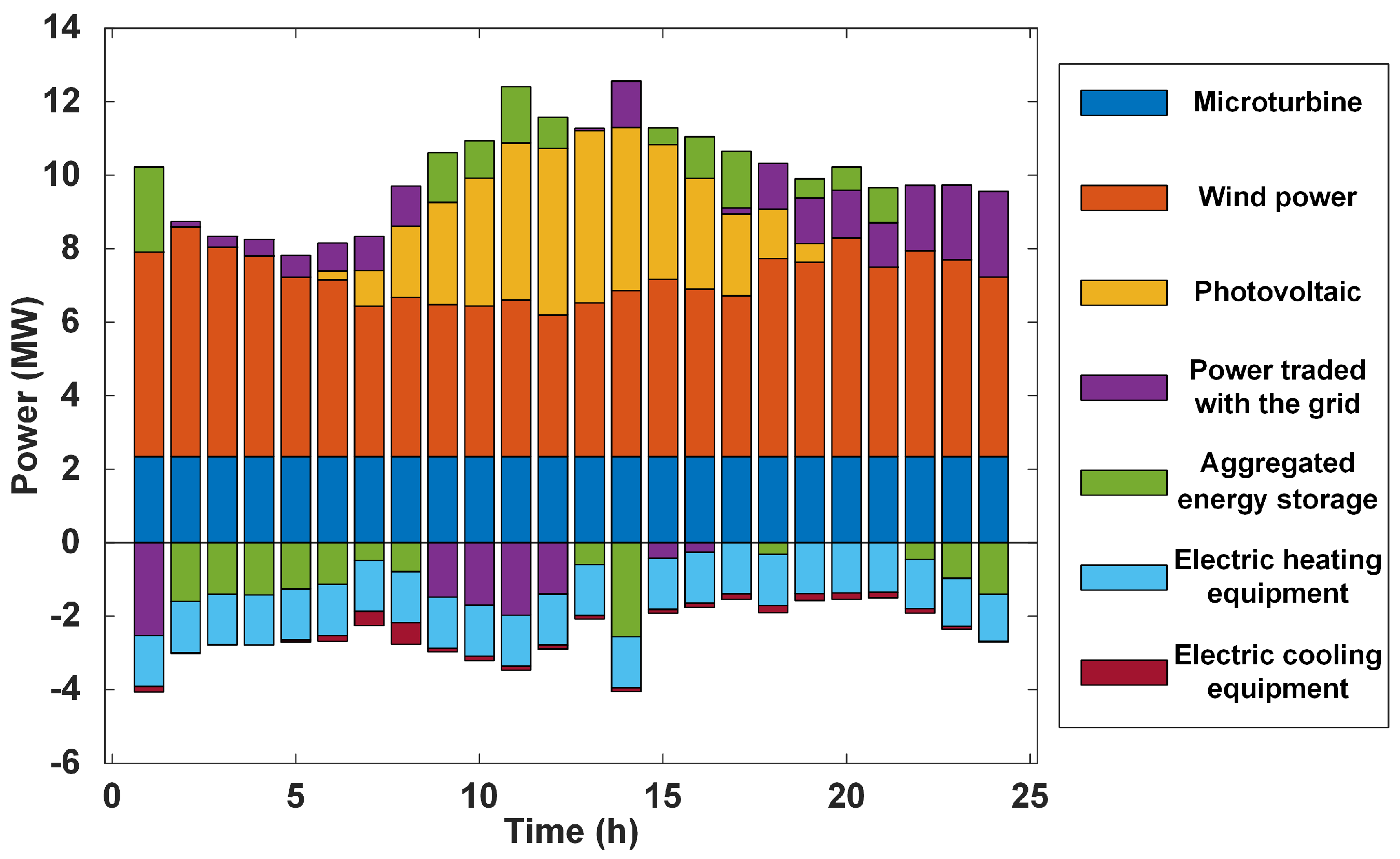
Figure 7, Figure 8 and Figure 9 illustrate the power balance of electrical, thermal, and cooling energy in Rural Area-1 of the simulation system. In the figures, positive values represent generated power, while negative values indicate power consumption other than the load. The sum of the two corresponds to the load condition. The results in Figure 7, Figure 8 and Figure 9 clearly demonstrate the coordinated operation of electricity, heating, and cooling networks under the proposed tri-carrier framework. The electrical balance shows that renewable generation and flexible loads are effectively scheduled to minimize grid exchange and curtailment. The thermal and cooling balances further reveal strong coupling between carriers—heat and cooling production dynamically shift between electric and thermal sources depending on energy availability.

Figure 10 and Figure 11, respectively, depict the electrical power balance in Rural Area-2 and Rural Area-3. Each rural area prioritizes dispatching WP and PV for electricity generation, reducing wind and solar curtailment while also lowering the cost of purchased electricity. Comparing the optimization results of each rural area, the outcomes for the three rural areas are not entirely consistent. The primary reason is that each rural area is located on different power grid and thermal network nodes, and there is a significant disparity in the loads across these regions. The distribution network operator conducts global optimization based on ensuring the security of the energy network and provides different feedback to each rural area. The three rural areas, based on the different feedback information and in conjunction with the capacity of internal equipment within their respective transformer districts, adjust their strategies to obtain final optimization results that are optimal for themselves while also ensuring the security of the distribution network.

5. Conclusions

This study proposes a hierarchical collaborative optimization method for RDES considering energy storage aggregation. The model enables cost-effective, privacy-preserving, and secure coordination among multiple rural energy districts while maintaining the stability of electrical and thermal networks. Validation on an IEEE 33-node electrical and 6-node thermal system confirms its effectiveness and scalability.

(1)

The Minkowski sum and inner approximation methods effectively aggregate heterogeneous ES-type resources into a unified flexibility model, achieving linearized computation with less than 10% flexibility loss.

(2)

The proposed hierarchical optimization model reduces overall operational costs while preserving participant privacy. After 33 iterations, all entities converge to stable and minimal operational costs.

(3)

The hierarchical framework enhances cost sharing and cooperation among entities, improving their willingness to participate in coordinated scheduling.

Despite promising simulation results, real-time implementation may face challenges such as communication delays, data uncertainty, and coordination errors. Future work will focus on larger-scale and real-world RDES applications, incorporating seasonal variations, renewable fluctuations, and stochastic demands, as well as exploring real-time, data-driven prediction and hardware-in-the-loop validation.

References

1. Fu, X.; Zhou, Y. Collaborative optimization of PV greenhouses and clean energy systems in rural areas. IEEE Trans. Sustain. Energy 2022, 14, 642–656. [Google Scholar] [CrossRef]
2. Nadeem, T.B.; Siddiqui, M.; Khalid, M.; Asif, M. Distributed energy systems: A review of classification, technologies, applications, and policies. Energy Strategy Rev. 2023, 48, 101096. [Google Scholar] [CrossRef]
3. Harish, V.; Anwer, N.; Kumar, A. Applications, planning and socio-techno-economic analysis of distributed energy systems for rural electrification in India and other countries: A review. Sustain. Energy Technol. Assess. 2022, 52, 102032. [Google Scholar] [CrossRef]
4. Anvari, S.; Medina, A.; Merchán, R.P.; Hernández, A.C. Sustainable solar/biomass/energy storage hybridization for enhanced renewable energy integration in multi-generation systems: A comprehensive review. Renew. Sustain. Energy Rev. 2025, 223, 115997. [Google Scholar] [CrossRef]
5. Huang, W.; Zhang, N.; Cheng, Y.; Yang, J.; Wang, Y.; Kang, C. Multienergy networks analytics: Standardized modeling, optimization, and low carbon analysis. Proc. IEEE 2020, 108, 1411–1436. [Google Scholar] [CrossRef]
6. Marlés-Sáenz, E.; Gómez-Luna, E.; Guerrero, J.M.; Vasquez, J.C. Analysis of impacts in electric power grids due to the integration of distributed energy resources. Energies 2025, 18, 745. [Google Scholar] [CrossRef]
7. Li, H.; Qin, B.; Wang, S.; Ding, T.; Liu, J.; Wang, H. Aggregate power flexibility of multi-energy systems supported by dynamic networks. Appl. Energy 2025, 377, 124565. [Google Scholar] [CrossRef]
8. Hinkelman, K.; Flores Garcia, J.D.; Anbarasu, S.; Zuo, W. A Review of Multi-Energy Systems from Resiliency and Equity Perspectives. Energies 2025, 18, 4536. [Google Scholar] [CrossRef]
9. Izadi, M.; Afsharpanah, F.; Mohadjer, A.; Shobi, M.O.; Ajarostaghi, S.S.M.; Minelli, F. Performance enhancement of a shell-and-coil ice storage enclosure for air conditioning using spiral longitudinal fins: A numerical approach. Heliyon 2025, 11, e42786. [Google Scholar] [CrossRef]
10. Müller, F.L.; Szabó, J.; Sundström, O.; Lygeros, J. Aggregation and disaggregation of energetic flexibility from distributed energy resources. IEEE Trans. Smart Grid 2017, 10, 1205–1214. [Google Scholar] [CrossRef]
11. Hussain, A.; Bui, V.H.; Kim, H.M. Microgrids as a resilience resource and strategies used by microgrids for enhancing resilience. Appl. Energy 2019, 240, 56–72. [Google Scholar] [CrossRef]
12. Fichera, A.; Marrasso, E.; Martone, C.; Pallotta, G.; Sasso, M.; Volpe, R. Ten questions concerning Renewable Energy Communities. Build. Environ. 2025, 281, 113193. [Google Scholar] [CrossRef]
13. Liu, P.; Ding, T.; Zou, Z.; Yang, Y. Integrated demand response for a load serving entity in multi-energy market considering network constraints. Appl. Energy 2019, 250, 512–529. [Google Scholar] [CrossRef]
14. Lu, S.; Gu, W.; Zhang, C.; Meng, K.; Dong, Z. Hydraulic-thermal cooperative optimization of integrated energy systems: A convex optimization approach. IEEE Trans. Smart Grid 2020, 11, 4818–4832. [Google Scholar] [CrossRef]
15. Li, Y.; Zou, Y.; Tan, Y.; Cao, Y.; Liu, X.; Shahidehpour, M.; Tian, S.; Bu, F. Optimal stochastic operation of integrated low-carbon electric power, natural gas, and heat delivery system. IEEE Trans. Sustain. Energy 2017, 9, 273–283. [Google Scholar] [CrossRef]
16. Zhou, B.; Xu, D.; Li, C.; Chung, C.Y.; Cao, Y.; Chan, K.W.; Wu, Q. Optimal scheduling of biogas–solar–wind renewable portfolio for multicarrier energy supplies. IEEE Trans. Power Syst. 2018, 33, 6229–6239. [Google Scholar] [CrossRef]
17. Li, C.; Yang, H.; Shahidehpour, M.; Xu, Z.; Zhou, B.; Cao, Y.; Zeng, L. Optimal planning of islanded integrated energy system with solar-biogas energy supply. IEEE Trans. Sustain. Energy 2019, 11, 2437–2448. [Google Scholar] [CrossRef]
18. Mancò, G.; Tesio, U.; Guelpa, E.; Verda, V. A review on multi energy systems modelling and optimization. Appl. Therm. Eng. 2024, 236, 121871. [Google Scholar] [CrossRef]
19. Soussi, A.; Zero, E.; Bozzi, A.; Sacile, R. Enhancing energy systems and rural communities through a system of systems approach: A comprehensive review. Energies 2024, 17, 4988. [Google Scholar] [CrossRef]
20. Li, J.; Zhang, M.; Shuai, Z.; Liu, H.; Li, B.; Zhang, C.; Zhu, L. Two-stage hybrid optimization of aggregated distributed generalized energy storages for complete uncertainty elimination. IEEE Trans. Smart Grid 2025, 16, 2075–2086. [Google Scholar] [CrossRef]
21. Xing, K.; Luo, L.; Lu, S.; Gu, W.; Wang, X.; Bai, Y. Improve operational flexibility of distribution systems using transportable resources. Renew. Sustain. Energy Rev. 2024, 204, 114788. [Google Scholar] [CrossRef]
22. Kang, W.; Chen, M.; Li, Q.; Lai, W.; Luo, Y.; Tavner, P.J. Distributed optimization model and algorithms for virtual energy storage systems using dynamic price. J. Clean. Prod. 2021, 289, 125440. [Google Scholar] [CrossRef]
23. Öztürk, E.; Rheinberger, K.; Faulwasser, T.; Worthmann, K.; Preißinger, M. Aggregation of demand-side flexibilities: A comparative study of approximation algorithms. Energies 2022, 15, 2501. [Google Scholar] [CrossRef]
24. Yi, Z.; Xu, Y.; Gu, W.; Yang, L.; Sun, H. Aggregate operation model for numerous small-capacity distributed energy resources considering uncertainty. IEEE Trans. Smart Grid 2021, 12, 4208–4224. [Google Scholar] [CrossRef]
25. Zhao, L.; Zhang, W.; Hao, H.; Kalsi, K. A geometric approach to aggregate flexibility modeling of thermostatically controlled loads. IEEE Trans. Power Syst. 2017, 32, 4721–4731. [Google Scholar] [CrossRef]
26. Han, J.; Liu, N.; Catalão, J.P. Optimization of distribution network and mobile network with interactive balance of flexibility and power. IEEE Trans. Power Syst. 2022, 38, 2512–2524. [Google Scholar] [CrossRef]
27. Yi, Z.; Xu, Y.; Gu, W.; Wu, W. A multi-time-scale economic scheduling strategy for virtual power plant based on deferrable loads aggregation and disaggregation. IEEE Trans. Sustain. Energy 2019, 11, 1332–1346. [Google Scholar] [CrossRef]
28. Zheng, W.; Lu, H.; Zhang, M.; Wu, Q.; Hou, Y.; Zhu, J. Distributed energy management of multi-entity integrated electricity and heat systems: A review of architectures, optimization algorithms, and prospects. IEEE Trans. Smart Grid 2023, 15, 1544–1561. [Google Scholar] [CrossRef]
29. Gao, H.; Li, Z. A benders decomposition based algorithm for steady-state dispatch problem in an integrated electricity-gas system. IEEE Trans. Power Syst. 2021, 36, 3817–3820. [Google Scholar] [CrossRef]
30. Chen, B.; Wu, W.; Lin, C.; Sun, H. Coordination of electricity and natural gas systems: An incentive-compatible mutual trust solution. IEEE Trans. Power Syst. 2020, 36, 2491–2502. [Google Scholar] [CrossRef]
31. Xuan, A.; Shen, X.; Guo, Q.; Sun, H. A conditional value-at-risk based planning model for integrated energy system with energy storage and renewables. Appl. Energy 2021, 294, 116971. [Google Scholar] [CrossRef]
32. Chen, S.; Conejo, A.J.; Wei, Z. Gas-power coordination: From day-ahead scheduling to actual operation. IEEE Trans. Power Syst. 2021, 37, 1532–1542. [Google Scholar] [CrossRef]
33. Zheng, Y.; Song, Y.; Hill, D.J.; Zhang, Y. Multiagent system based microgrid energy management via asynchronous consensus ADMM. IEEE Trans. Energy Convers. 2018, 33, 886–888. [Google Scholar] [CrossRef]
34. Zhang, Z.; Wang, Y.; Wang, C.; Su, Y.; Wang, Y.; Dai, Y.; Cui, C.; Zhang, W. Distributed Chance-Constrained Optimal Dispatch for Integrated Energy System With Electro-Thermal Couple and Wind-Storage Coordination. IEEE Trans. Ind. Appl. 2024, 61, 833–846. [Google Scholar] [CrossRef]
35. Ma, Z.; Zhou, Y.; Zheng, Y.; Yang, L.; Wei, Z. Distributed robust optimal dispatch of regional integrated energy systems based on ADMM algorithm with adaptive step size. J. Mod. Power Syst. Clean Energy 2023, 12, 852–862. [Google Scholar] [CrossRef]
Figure 1. Diagram of the proposed hierarchical coordinated optimization framework for RDES.
Electronics 14 04473 g001
Figure 2. The hierarchical distributed scheduling flowchart.
Electronics 14 04473 g002
Figure 3. The topological structure of the RDES used in this paper.
Electronics 14 04473 g003
Figure 4. Maximum predicted output of various loads and new energy sources in rural transformer districts.
Electronics 14 04473 g004
Figure 5. Comparison of theoretical maximum output of ES-type resources before and after aggregation.
Electronics 14 04473 g005
Figure 6. Changes in operational costs of each participating entity during the iteration process.
Electronics 14 04473 g006
Figure 7. Electrical power balance in Rural Area-1.
Electronics 14 04473 g007
Figure 8. Thermal power balance in Rural Area-1.
Electronics 14 04473 g008
Figure 9. Cooling power balance in Rural Area-1.
Electronics 14 04473 g009
Figure 10. Electrical power balance in Rural Area-2.
Electronics 14 04473 g010
Figure 11. Electrical power balance in Rural Area-3.
Electronics 14 04473 g011