Article

UnderFSL: Boundary-Preserving Undersampling with Few-Shot Relation Networks for Cross-Machine CNC Fault Diagnosis

1
Artificial Intelligence Research Center, Korea Electrotechnology Research Institute, Changwon 51543, Republic of Korea
2
Department of Artificial Intelligence, Chung-Ang University, Seoul 06974, Republic of Korea
*
Author to whom correspondence should be addressed.
Electronics 2025, 14(18), 3699; https://doi.org/10.3390/electronics14183699
Submission received: 4 September 2025 / Revised: 12 September 2025 / Accepted: 15 September 2025 / Published: 18 September 2025

Abstract

Fault diagnosis in Computer Numerical Control (CNC) machines remains challenging due to severe class imbalance, scarcity of fault data, and distribution shifts across machines. This paper introduces Undersampling-based Few-shot Learning (UnderFSL), a simple yet effective framework that integrates strategic undersampling using Condensed Nearest Neighbor (U-CNN) with a Relation Network few-shot classifier. The proposed method first transforms raw 1D vibration signals into 2D Continuous Wavelet Transform (CWT) scalograms to capture time–frequency structure and then reduces the majority (normal) class using U-CNN, yielding a compact set of boundary-informative prototypes while alleviating imbalance. Finally, a Relation Network is trained in an episodic FSL regime on the balanced set to support cross-machine generalization. On the Bosch CNC machining benchmark under leave-one-machine-out validation, UnderFSL attains a macro F1-Score of 0.96, an accuracy of 0.96, a recall of 0.92, and a precision of 1.00, surpassing traditional and standard deep baselines. The results suggest that boundary-preserving undersampling combined with metric learning provides a robust and scalable path for industrial fault diagnosis when fault data are extremely limited.

1. Introduction

1.1. Industrial Motivation and Background

The paradigm shift toward Smart Manufacturing is characterized by the integration of data-driven intelligence into manufacturing systems to enhance efficiency and autonomy. Computer Numerical Control (CNC) machines remain the backbone of modern manufacturing, which are prized for their precision and automation. However, their complex and high-speed operations make them susceptible to various failures, such as tool breakage, improper clamping, and chip jamming [1]. Unanticipated failures lead to significant production downtime, increased operational costs, and compromised product quality. Therefore, the development of intelligent, reliable, and scalable fault diagnosis systems is paramount for ensuring the stability and efficiency of manufacturing processes.
Data-driven approaches, particularly those based on deep learning, have shown considerable promise in fault diagnosis by facilitating the learning of complex patterns from sensor data [2]. However, the deployment of these models in real-world industrial environments faces several persistent challenges that limit their effectiveness and scalability.

1.2. Challenges and Limitations of Existing Research

The primary obstacles in industrial fault diagnosis stem from two interconnected challenges: data characteristics and model generalization. First, industrial datasets are inherently imbalanced. As failures are rare events, normal operation data overwhelmingly exceeds fault operation data. Models trained on such skewed data tend to be biased toward the majority class, resulting in poor detection performance for critical faults [3]. Furthermore, acquiring labeled fault data is often expensive and time-consuming, leading to scenarios where fault data is not just imbalanced but extremely scarce. Second, the dynamic nature of production environments leads to feature drift. Data distributions can shift over time due to machine aging or maintenance. Moreover, discrepancies often exist even among identical types of machines due to minor variations in hardware or operating conditions [4], making it difficult for a model trained on one machine (source domain) to generalize to another machine (target domain).
Traditional machine learning methods often struggle with the high dimensionality of sensor data. While deep learning models such as Convolutional Neural Networks (CNNs) and Autoencoders can learn powerful features, they typically require large volumes of balanced, labeled data [5].
In industrial fault diagnosis, fault data is often extremely scarce, making Few-Shot Learning (FSL) a promising paradigm [6]. Metric-based FSL models learn transferable embedding spaces where new data can be classified using only a few support examples [7]. Yet, data scarcity is frequently coupled with class imbalance—another critical challenge in industrial fault diagnosis [8]. While FSL mitigates scarcity and undersampling alleviates imbalance, their integration remains underexplored. The effectiveness of metric-based FSL ultimately depends on the quality of its embedding space, which is shaped by the training distribution. Poor undersampling choices risk discarding boundary-critical samples, thereby weakening discriminative feature learning. In particular, how to optimally combine undersampling with FSL to preserve discriminative embedding quality under feature drift has not been systematically investigated.

1.3. Main Contributions

To address these limitations, this paper proposes a novel and robust fault diagnosis framework that synergistically combines effective feature representation, strategic data balancing, and advanced metric learning. A primary contribution of this study is the development of an integrated framework that tackles the dual challenge of data scarcity (for faults) and data abundance (for normal operations) by combining strategic undersampling with Relation Network-based deep metric learning. Furthermore, we systematically optimize the undersampling strategy for the FSL environment by comparing Random, Condensed Nearest Neighbor (U-CNN), and Instance Hardness Threshold (IHT) techniques. This analysis experimentally demonstrates a significant synergy when the boundary-preserving U-CNN technique is combined with the Relation Network’s learning mechanism. The framework leverages a robust time–frequency feature representation utilizing the Continuous Wavelet Transform (CWT) with the Morlet wavelet, which is known for its effectiveness with non-stationary signals [9], extracting 2D scalogram features from vibration signals, optimized for FSL-based diagnosis. Finally, the proposed framework is rigorously validated on the Bosch CNC Machining benchmark dataset under a challenging cross-machine validation strategy, demonstrating superior generalization performance.

1.4. Organization of the Paper

The remainder of this paper is organized as follows: Section 2 formulates the problem. Section 3 details the proposed methodology. Section 4 presents the experimental setup, results, and analysis. Section 5 discusses the industrial implications and limitations. Finally, Section 6 concludes the paper.

2. Preliminaries and Problem Formulation

2.1. System Description

The target system involves 4-axis horizontal CNC machining centers processing aluminum workpieces. The monitoring system utilizes indirect measurement via tri-axial accelerometers mounted on the spindle housing. The primary goal is to detect process failures (NOK), distinguishing them from healthy processes (OK). The data consists of time-series vibration signals collected at a sampling rate of 2 kHz [4].

2.2. Problem Formulation: Imbalanced Few-Shot Fault Diagnosis

We address the problem of fault diagnosis under the constraints of severe class imbalance and data scarcity in a cross-machine setting.
Let the source domain training dataset be D train = { ( x i , y i ) } i = 1 N train , where x i is the input signal and y i C = { C OK , C NOK } is the corresponding label. The dataset is highly imbalanced, meaning the number of samples in the normal class N OK is significantly larger than the number of samples in the fault class N NOK ( N OK N NOK ).
The objective is to learn a classifier f θ that can generalize well to a target domain test dataset D test , collected from different machines, which implies a potential distribution shift. We approach this using an FSL paradigm. FSL training utilizes an episodic approach. A typical FSL task is defined as an N-way K-shot problem. In our binary classification scenario ( N = 2 ), the goal is to correctly classify new query samples given only K labeled examples (the support set) for each class. The challenge lies in effectively balancing D train to learn a robust feature representation while simultaneously training the model to perform accurate classification with only K fault examples, especially when K is very small (e.g., K = 3 ).

3. Proposed Methodology

In this study, to simultaneously solve the problems of data imbalance and scarcity, we propose Undersampling-based Few-shot Learning (UnderFSL), a novel fault diagnosis framework that combines undersampling with FSL. As summarized in Figure 1, UnderFSL consists of three core stages. First, the raw 1D vibration signals are transformed into 2D scalogram images using the CWT. Second, to address the data imbalance problem, we apply strategic undersampling to the majority class (normal data). Finally, the preprocessed data is fed into a Relation Network-based FSL model to classify the final fault status.

3.1. Time–Frequency Feature Representation via CWT

Vibration data collected from CNC machines are inherently non-stationary signals [10]. Fault events often manifest as transient, localized energy bursts in specific frequency bands. CWT is ideal for analyzing such signals as it provides a high-resolution time–frequency representation [11].
The CWT of a signal x ( t ) is calculated by convolving it with scaled and shifted versions of a mother wavelet ψ ( t ) :
W ( a , b ) = 1 | a | x ( t ) ψ t b a d t
where a is the scale parameter (inversely related to frequency), b is the translation parameter (related to time), and  ψ ( · ) is the complex conjugate of the mother wavelet. The resulting CWT coefficients W ( a , b ) form a 2D map known as a scalogram.
For the CWT, the Morlet wavelet was chosen as the mother wavelet. The Morlet wavelet is a complex-valued wavelet composed of a complex sinusoid modulated by a Gaussian envelope. This structure makes it highly effective for capturing transient events and frequency variations characteristic of mechanical faults, due to its similarity to the oscillatory nature of vibration signals. It provides an optimal balance between time and frequency resolution [12,13].
The 1D vibration signals from each of the X, Y, and Z axes are transformed into respective 2D scalograms via CWT and then resampled to generate images with a resolution of 64 × 64 pixels. This resolution is an optimized value to preserve essential fault features while ensuring the computational efficiency of the subsequent deep learning model.

3.2. Undersampling Techniques for Data Balancing

Strategic undersampling techniques, such as IHT and U-CNN, rely on specific criteria within a defined feature space, such as distance calculations, neighborhood analysis, or hardness estimations. Applying these directly to the high-dimensional CWT scalograms ( 64 × 64 × 3 ) can be computationally inefficient and susceptible to the curse of dimensionality. To address this, we employed a separate 2D Convolutional Autoencoder (CAE), pre-trained on the CWT images, to extract a meaningful, lower-dimensional latent representation suitable for undersampling.
The implemented CAE architecture has input and output dimensions of 64 × 64 × 3 . The encoder consists of four convolutional blocks, each comprising a 2D convolution layer with a 3 × 3 kernel, followed by Batch Normalization and a ReLU activation function. Downsampling is performed using a stride of 2 in each block. The number of filters for the four blocks is 64, 128, 192, and 192, respectively, resulting in a bottleneck feature map of size 4 × 4 × 192 . We then apply Global Average Pooling (GAP) to this feature map to obtain a 192-dimensional compact feature vector [14]. GAP was chosen as it effectively generates a representative feature vector with fewer parameters than a fully connected layer, thus enhancing computational efficiency. The decoder mirrors the encoder architecture, employing transposed convolutions with a 3 × 3 kernel and a stride of 2 for upsampling and reconstructing the original image. The CAE was pre-trained on the M01 training set using Mean Squared Error (MSE) loss. Training was performed for 100 epochs with the Adam optimizer, using a learning rate of 0.001 and a batch size of 32. All subsequent undersampling algorithms (Random, IHT, U-CNN) were executed using these 192-dimensional vectors generated by the trained encoder to determine which samples to retain.
To mitigate the model’s bias toward the majority class, we applied undersampling to the majority class (normal data) in the training set. This study systematically compares and analyzes three different undersampling techniques, based on their use of information, to determine the most effective approach for the FSL framework. To facilitate a direct comparison with U-CNN, which we hypothesize to have the strongest synergy with our FSL model, the target ratio for Random Undersampling was set to 2:1, mirroring the approximate balance inherently achieved by the U-CNN algorithm.
  • Random Undersampling: This method randomly removes samples from the majority class until the target class ratio is reached. While widely used for its simplicity, it risks discarding potentially informative data [15]. Mathematically, this is equivalent to randomly selecting a subset D maj D maj from the majority class dataset D maj that satisfies | D maj | = r · | D min | , according to a target ratio r.
  • Instance Hardness Thresholding: This technique removes ’hard’ majority class samples, which are consistently misclassified by multiple classifiers, considering them as noise or overlapping data [16]. The Instance Hardness I H ( x ) for each majority class sample x D maj is given by Equation (2).
    I H ( x ) = 1 M i = 1 M I ( C i ( x ) L ( x ) )
    Here, L ( x ) is the true label of sample x, M is the number of classifiers, and  I ( · ) is the indicator function. Samples with an I H ( x ) higher than a predefined threshold t are removed, ultimately producing D maj = { x D maj I H ( x ) t } .
  • Condensed Nearest Neighbor Undersampling: U-CNN aims to find a minimal subset of the majority class that retains the classification performance for the minority class [17]. As described in Algorithm 1, the procedure begins by initializing a store, S, containing all minority class samples ( D min ). It then iteratively reviews all majority class samples ( D maj ) and adds a sample to the store S only if a 1-NN classifier, using only the current data in S, misclassifies that sample. This process is repeated until no more samples can be added to the store, and the final resulting set S consists of high-value, informative samples located primarily near the decision boundaries between classes.
Considering the characteristics of these techniques, we hypothesize that U-CNN undersampling, in particular, will have a strong synergy with metric-based FSL models. Unlike IHT and random undersampling, U-CNN preserves the essential information required to define the class boundaries. The preserved boundary information provides the critical context for the FSL model to learn a discriminative metric space separating the normal and fault classes, thereby focusing the learning process on the most challenging examples.
Algorithm 1 Condensed Nearest Neighbor
  1:Input:  D min (set of minority class samples), D maj (set of majority class samples)
  2:Output: S (the condensed training set)
  3:
  4: S D min
  5: C D maj                                                        ▹ Create a candidate set from D maj
  6: has _ changed true
  7:
  8:while  has _ changed  do
  9:     has _ changed false
10:    for each sample x in C do
11:        Find x nn , the nearest neighbor of x in S
12:        if label(x) ≠ label( x nn ) then
13:            S S { x }                                             ▹ Add misclassified sample to S
14:            C C { x }                                               ▹ Remove x from candidates
15:            has _ changed true
16:        end if
17:    end for
18:end while
19:
20:return S

3.3. Relation Network for Fault Diagnosis

For the core classification task, we employed the Relation Network, a state-of-the-art metric-based FSL architecture [18]. The key advantage of the Relation Network over other FSL methods (e.g., Prototypical Networks) is its ability to learn a flexible, deep non-linear metric to compare samples, rather than relying on fixed metrics like Euclidean distance [18,19]. This is particularly powerful for complex data like scalogram images, where the differences between normal and fault states can be subtle and non-linear.
  • Episodic Training Paradigm: FSL models are trained in an episodic manner [20]. In each training episode, we construct a small Support Set S and a Query Set Q from the (undersampled) training data. We adopted a 2-way 3-shot setting. This corresponds to our binary classification problem (2-way: Normal vs. Abnormal). The 3-shot setting was chosen to reflect the extreme scarcity of fault data in real-world scenarios. The support set S consists of 3 examples from the normal class and 3 examples from the abnormal class.
  • Relation Network Architecture: As shown in Figure 2, the Relation Network consists of two main modules. The detailed architecture, including specific layer configurations and output shapes, is provided in Table 1.
    -
    Embedding Module ( f ϕ ): This module is a CNN-based backbone that maps the input images (scalograms) into high-dimensional feature embeddings. We utilized a CNN architecture for feature extraction from the 64 × 64 input images.
    -
    Relation Module ( g φ ): This module calculates a similarity score, termed the relation score. For a given class C i , the support features are aggregated (e.g., by element-wise sum or averaging). This aggregated feature representation f ϕ ( S i ) is then concatenated with the query feature f ϕ ( Q j ) . This concatenated feature block is fed into the relation module g φ (another neural network), which outputs a relation score r i , j between 0 and 1, indicating the similarity between the query Q j and the class C i .
r i , j = g φ ( Concat [ f ϕ ( S i ) , f ϕ ( Q j ) ] )
  • Optimization: The model is trained end-to-end to optimize the parameters ϕ and φ . The objective is to maximize the relation score for matching pairs and minimize it for mismatching pairs. The Mean Squared Error (MSE) loss function is used:
    L = i , j ( r i , j I ( y i = y j ) ) 2
    where I ( · ) is an indicator function that equals 1 if the labels match, and 0 otherwise. By optimizing this objective, both the embedding module f ϕ and the relation module g φ learn the most effective way to represent and compare the samples for the given task.

4. Experimental Validation and Results

4.1. Dataset Description: Bosch CNC Machining Benchmark

We utilized the Bosch CNC Machining Dataset [4]. This dataset was collected from three different 4-axis horizontal CNC machines (M01, M02, M03) during the processing of aluminum workpieces over a two-year period. The dataset includes accelerometer data sampled at 2 kHz, with labels for normal and faulty processes across 15 different tool operations (OPs). Crucially, the dataset explicitly incorporates real-world challenges such as cross-machine and cross-time feature drift, and significant class imbalance. In this study, to clearly and rigorously evaluate the cross-machine generalization performance, we focused our experiments on OP07, the only tool operation for which complete normal and fault data exist across all three machines (M01, M02, and M03).

4.2. Experimental Setup and Implementation Details

To rigorously test the model’s generalization capability—a key requirement for scalable industrial deployment—we adopted a strict machine-wise splitting strategy for the OP07 data. The model was trained exclusively on OP07 data from Machine 1 (M01). The test set comprised all available OP07 data from M01, M02, and M03. This cross-machine validation setup directly evaluates the model’s performance on unseen machines (M02, M03) and its robustness against feature drift.
The framework was implemented using the PyTorch 3.8 library, and all experiments were conducted on a workstation equipped with an NVIDIA GeForce RTX 4090 GPU. The feature encoder and the relation network share the same optimization settings. Both modules were trained with the Adam optimizer with an initial learning rate of 0.001, and a StepLR scheduler was applied to decrease the learning rate by a factor of 0.5 ( γ = 0.5 ) every 500 steps. The model followed the 2-way 3-shot paradigm for 1000 training episodes.

4.3. Evaluation Metrics

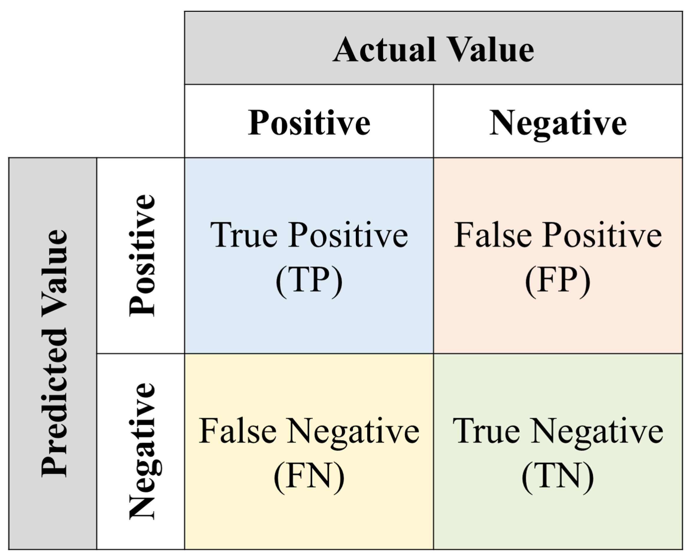
Due to the inherent class imbalance in the dataset, accuracy alone is an insufficient metric. Therefore, to comprehensively evaluate the model’s performance, we employed four standard metrics calculated from the confusion matrix components, as shown in Figure 3: True Positives (TP), True Negatives (TN), False Positives (FP), and False Negatives (FN). In this context, the positive class refers to the fault state (NOK). Accuracy measures the overall proportion of correctly classified instances. Precision evaluates the reliability of the positive predictions, where high precision indicates a low false alarm rate. Recall (or sensitivity) measures the ability to identify all actual positive instances, which is crucial for minimizing missed faults. The F1-Score provides a single, balanced metric by calculating the harmonic mean of precision and recall. The formulas for these metrics are as follows:
Accuracy = T P + T N T P + T N + F P + F N
Precision = T P T P + F P
Recall = T P T P + F N
F 1- Score = 2 · Precision · Recall Precision + Recall

4.4. Analysis of Undersampling Effects

To understand how different undersampling strategies affect the distribution of the training data (M01) within the learned latent space, we visualized the results. As detailed in Section 3.2, undersampling was performed on feature vectors obtained by applying GAP to the latent space of the pre-trained 2D CAE. Figure 4 illustrates the original imbalanced data distribution in this latent space and the resulting distributions after applying Random, IHT, and U-CNN undersampling.
Figure 4a shows the original dataset distribution within the CAE’s latent space. It highlights the severe class imbalance where the majority class (Normal/OK, blue) overwhelmingly dominates the minority class (Abnormal/NOK, red).
Figure 4b illustrates the effect of Random Undersampling. While the data balance is achieved (2:1 ratio), the selection process is arbitrary within the latent space. This results in a sparse distribution where potentially informative samples near the latent decision boundary might have been discarded.
Figure 4c shows the result of IHT undersampling. Executed in this latent space, IHT aims to remove samples identified as having high instance hardness (often noisy or overlapping samples). The visualization suggests that IHT may clean up the distribution but could inadvertently discard challenging boundary samples crucial for learning a robust metric space.
In contrast, Figure 4d demonstrates the effectiveness of U-CNN within this latent space. By calculating nearest neighbors based on the latent representation, U-CNN selectively retains majority class samples that are critical for defining the decision boundary (i.e., those closest to the minority class). The visualization clearly shows that the remaining majority samples are located adjacent to the minority samples. This boundary-preserving selection ensures that the most informative examples are retained for the subsequent FSL training, supporting our hypothesis (Section 3.2).

4.5. Baseline Comparisons

To evaluate the performance of the proposed UnderFSL model, we compared it against several baseline models representing two distinct approaches: those utilizing handcrafted statistical features and those leveraging deep learning on scalogram images. The time-series statistical features extracted from the raw signals included mean, standard deviation, Root Mean Square (RMS), skewness, kurtosis, and crest factor.
The first approach relies on traditional methods using these statistical features. Within this category, we utilized the Support Vector Machine (SVM) [21], a well-established classifier known for finding optimal separating hyperplanes. To ensure a comprehensive comparison, we evaluated SVMs trained on both the original imbalanced data and data balanced by the three undersampling techniques (Random, IHT, U-CNN). Additionally, we included the Statistical Autoencoder (StatAE) [22], an unsupervised anomaly detection model. StatAE identifies faults by detecting high reconstruction errors for inputs differing from the normal data distribution it was trained on. A test sample is identified as a fault if its reconstruction error exceeds a predefined threshold; since it is trained only on normal data, undersampling is not applicable.
The second approach employs deep learning-based methods that directly learn features from the scalogram images. As a standard supervised learning baseline to compare against the proposed FSL approach, we employed the VGG-7 classifier. This model is based on the VGG architecture [23], a well-validated CNN known for its simple yet effective structure of stacked 3 × 3 convolutional layers. The VGG-7 model is trained directly on the (resampled) training scalogram images to classify fault status.

4.6. Performance Analysis and Discussion

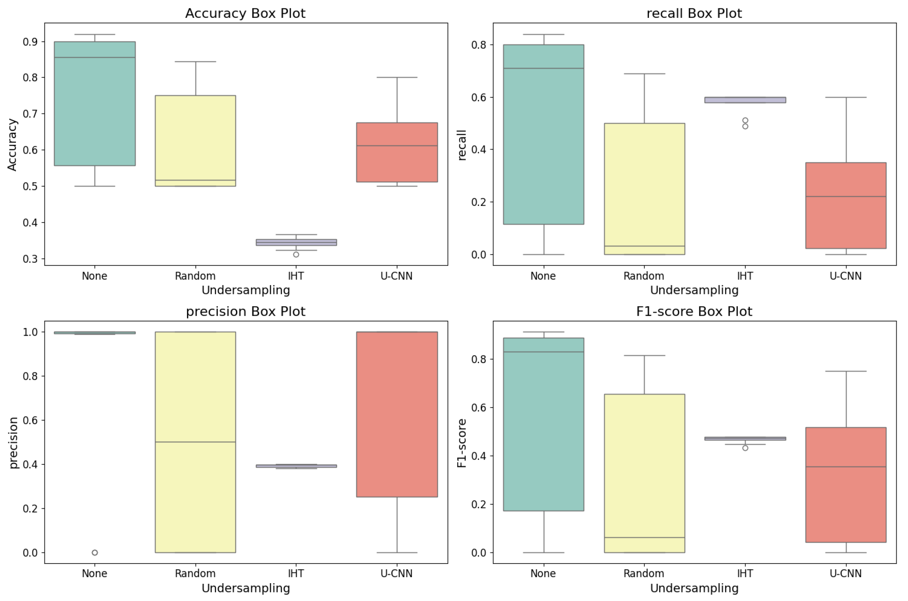
The comprehensive performance comparison of all models in the cross-machine validation scenario is summarized in Table 2. All experiments were repeated 10 times, and the results are reported as mean ± standard deviation. To thoroughly investigate the impact of different undersampling strategies on model performance and stability, we visualize the distribution of the results for each model in the following subsections.

4.6.1. Impact of Undersampling on Baseline Models

The impact of undersampling varied significantly across the baseline models, revealing fundamental differences in how traditional machine learning and standard deep learning approaches cope with data imbalance and feature drift. The SVM models, which relied on handcrafted statistical features, generally struggled in the cross-machine environment, as visualized in Figure 5. Without undersampling (None), the F1-Score was extremely low (0.07), indicating a failure to detect most faults due to the severe imbalance. Interestingly, IHT provided the most significant improvement in F1-Score (0.41) for SVM by improving recall (0.41). However, this improvement came at a substantial cost; the accuracy (0.37) and precision (0.43) were very low, suggesting an unacceptably high rate of false alarms. Overall, SVM performance remained insufficient, highlighting the limitations of handcrafted features under feature drift.
In contrast, the standard supervised deep learning model, VGGNet, utilized the richer information contained in CWT scalogram images. As illustrated in Figure 6, VGGNet achieved its highest average F1-Score (0.59) without undersampling. However, this metric masks a critical issue regarding stability: the performance distribution is extremely wide (standard deviation 0.39), indicating significant instability and poor generalization capability. Furthermore, applying undersampling strategies generally degraded the performance (e.g., F1-Score dropped to 0.32 with U-CNN). This suggests that standard CNN classifiers struggle to learn robust representations when the volume of training data (even if imbalanced) is reduced in a challenging cross-machine setting.

4.6.2. Synergy of Undersampling and Few-Shot Learning

In contrast to the baseline models, the proposed UnderFSL framework demonstrated a significant positive synergy with strategic undersampling, as visualized in Figure 7.
While the model maintained perfect precision (1.00) across all configurations—indicating an absence of false alarms—the recall and F1-Score improved drastically when balancing was applied. Random undersampling boosted the F1-Score from 0.59 (None) to 0.81. Crucially, the combination with U-CNN achieved the highest performance (F1-Score 0.96) with excellent stability (narrow distribution). This strongly supports our hypothesis (Section 3.2) that the boundary-preserving nature of U-CNN synergizes effectively with the Relation Network’s metric learning process, enabling it to learn a highly discriminative embedding space. Conversely, IHT degraded the performance (F1-Score 0.52), suggesting it might remove critical boundary samples essential for FSL.

4.6.3. Overall Performance Comparison and Stability

Figure 8 compares the best-performing configuration for each model type: UnderFSL(U-CNN), SVM(IHT), VGGNet(None), and StatAE.
The proposed UnderFSL(U-CNN) significantly outperformed all baseline methods. The visualization clearly highlights two major advantages. First, it achieved the highest median scores across all key metrics (Accuracy 0.96, F1-Score 0.96). Second, the Interquartile Range (IQR) of UnderFSL(U-CNN) is remarkably narrow, especially compared to VGGNet(None), indicating superior stability and reliability in the cross-machine validation scenario.
While the unsupervised StatAE achieved a high F1-Score (0.80) and perfect recall (1.00), it suffered from lower precision (0.67). This indicates a tendency to generate false alarms, which can be disruptive in industrial settings. In contrast, UnderFSL(U-CNN) successfully detected the vast majority of actual faults (Recall 0.92) while eliminating false alarms (Precision 1.00), proving its robustness and suitability for real-world deployment.

4.7. Feature Space and Error Analysis Visualization

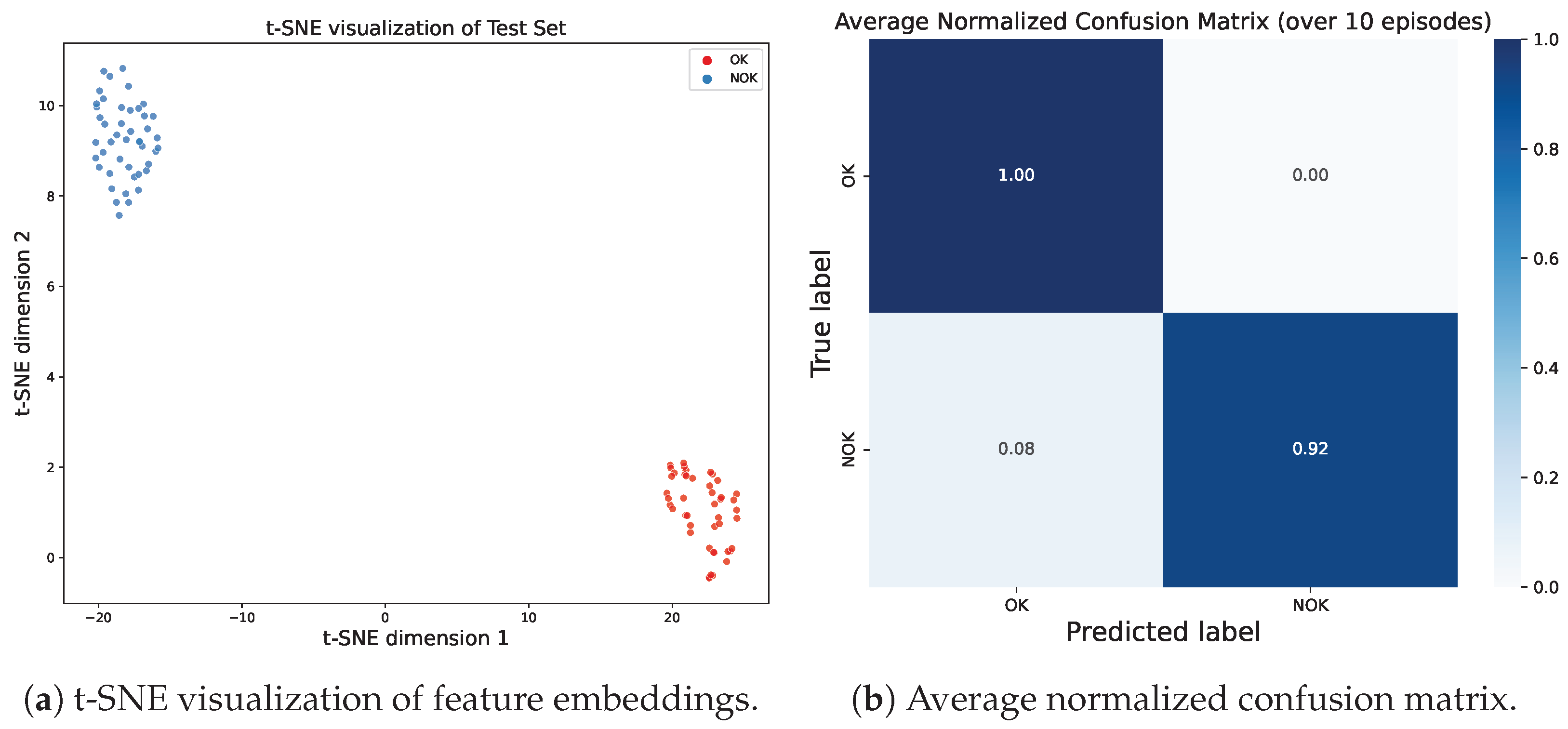
To further investigate the effectiveness of the proposed UnderFSL(U-CNN) model, we visualized the feature embeddings of the test data and the model’s classification performance. For this visualization, we employed t-Distributed Stochastic Neighbor Embedding (t-SNE), a non-linear dimensionality reduction technique widely used for visualizing high-dimensional data [24]. t-SNE maps high-dimensional data points to a two or three-dimensional space, representing similar objects as nearby points and dissimilar objects as distant points. Figure 9 provides a qualitative analysis of the capabilities of the model.
Figure 9a illustrates the distribution of the test set feature embeddings in a 2D space using t-SNE. The visualization clearly shows that the OK (normal, red) and NOK (abnormal, blue) classes form distinct, well-separated clusters. This provides strong visual evidence that the embedding module, synergized with U-CNN undersampling, has learned a highly discriminative and generalizable feature representation, which is a key factor in the model’s high performance.
Figure 9b presents the average normalized confusion matrix from 10 repeated test episodes. It quantitatively confirms the performance metrics detailed in Table 2. The matrix clearly shows a perfect precision score (1.00), as no normal samples were misclassified as abnormal (zero false positives), indicating the complete avoidance of false alarms. Furthermore, it visualizes the high recall rate (0.92), demonstrating the model’s capability to correctly identify 92% of the actual faults (minimizing missed detections). This combination of high recall and precision reinforces the model’s reliability, which is a critical requirement for practical industrial applications.

5. Industrial Implications and Discussion

5.1. Generalization Capability and Scalability

A key requirement for deploying fault diagnosis systems in smart manufacturing is scalability across multiple machines. Models must be robust against feature drift. Our experimental design rigorously tested this capability by training the model only on M01 and testing it on M02 and M03.
The success of the proposed framework (96% accuracy) in this challenging cross-machine test highlights its superior generalization capability. This suggests that the combination of CWT features, CNN undersampling, and the Relation Network’s learned metric is highly transferable. This robustness significantly reduces the effort required for model deployment and maintenance, as a single model can potentially monitor multiple CNC machines without extensive machine-specific retraining.
Furthermore, the scalability of practical deployment also depends on computational efficiency. To this end, we measured the inference speed on an NVIDIA GeForce RTX 4090 GPU and found that the trained model requires an average of only 4 ms to process a single query sample. This high efficiency further confirms the suitability of the proposed framework for real-time monitoring in industrial settings.

5.2. Addressing Data Scarcity in Practice

The reliance on 3-shot learning means that the system can be effectively trained or adapted to new conditions with only a handful of fault examples. This is a significant advantage in industrial settings where fault data is rare and expensive to acquire. The systematic integration of U-CNN undersampling effectively manages the overwhelming amount of normal data, ensuring the FSL model focuses on the most relevant information near the decision boundaries.

5.3. Limitations and Future Work

While the proposed framework demonstrates excellent performance, some limitations remain. The current model is trained to recognize fault types present in the training data; its performance on entirely novel, unseen fault types (a Zero-Shot Learning scenario) has not been evaluated. Additionally, while CWT proved effective, the computational cost of CWT preprocessing might be a concern for high-throughput real-time systems if higher resolutions are required.
Future work will focus on several directions to enhance the framework. We plan to explore semi-supervised FSL approaches to leverage the large amounts of unlabeled data more effectively. Additionally, we aim to extend the framework to multi-class fault diagnosis, enabling the identification of specific fault types, such as tool wear or chip jamming. Finally, we will investigate the integration of other sensor modalities, including acoustic emission and current data, to further enhance diagnostic robustness.

6. Conclusions

This paper proposed a novel and robust framework for CNC machine fault diagnosis, which is specifically designed to tackle the persistent challenges of severe class imbalance and feature drift found in real-world industrial data. Our approach successfully integrates the CWT for effective feature extraction from non-stationary vibration signals, strategic undersampling for balancing the training data, and a Relation Network-based FSL model for robust classification from scarce fault data.
Through rigorous experimentation on the Bosch CNC Machining benchmark dataset, using a challenging cross-machine validation strategy, we demonstrated the superiority of the proposed method. The combination of U-CNN undersampling and the Relation Network achieved an outstanding accuracy of 96%, a recall of 92%, and a perfect precision score of 1.00, as substantiated by the detailed comparative analysis in Section 4.6. This result not only significantly outperforms traditional SVM and Autoencoder-based methods but also validates the synergy between preserving boundary-defining samples via U-CNN undersampling and the deep metric learning capability of the Relation Network.
The high generalization performance on unseen machines proves the model’s robustness and its suitability for scalable deployment in real-world industrial environments, providing an effective solution for building reliable diagnostic systems even when fault data is extremely limited.

Author Contributions

Conceptualization, J.K. (Jonggeun Kim) and S.K.; methodology, J.K. (Jonggeun Kim); software, J.K. (Jonggeun Kim); validation, H.-U.L. and O.C.; formal analysis, J.K. (Jonggeun Kim) and J.K. (Jinyong Kim); investigation, J.K. (Jonggeun Kim); resources, H.-U.L. and J.K. (Jinyong Kim); data curation, J.K. (Jonggeun Kim) and J.K. (Jinyong Kim); writing—original draft preparation, J.K. (Jonggeun Kim) and S.K.; writing—review and editing, O.C. and H.-U.L.; visualization, J.K. (Jonggeun Kim); supervision, S.K.; project administration, J.K. (Jonggeun Kim); funding acquisition, S.K. All authors have read and agreed to the published version of the manuscript.

Funding

This research was supported by the Korea Electrotechnology Research Institute (KERI) Primary research program through the National Research Council of Science & Technology (NST) and funded by the Ministry of Science and ICT (MSIT) (No. 25A01053).

Data Availability Statement

Bosch CNC data used in this study are available at https://archive.ics.uci.edu/dataset/752/bosch+cnc+machining+dataset (accessed on 1 May 2023).

Acknowledgments

This research was supported by Korea Electrotechnology Research Institute (KERI) Primary research program through the National Research Council of Science & Technology (NST) funded by the Ministry of Science and ICT (MSIT) (No. 25A01053).

Conflicts of Interest

The authors declare no conflicts of interest.

Abbreviations

CAEConvolutional Autoencoder
CNCComputer Numerical Control
CNNConvolutional Neural Network
CWTContinuous Wavelet Transform
FSLFew-Shot Learning
GAPGlobal Average Pooling
IHTInstance Hardness Threshold
IQRInterquartile Range
MSEMean Squared Error
OPOperation
RMSRoot Mean Square
StatAEStatistical Autoencoder
SVMSupport Vector Machine
U-CNNCondensed Nearest Neighbor
UnderFSLUndersampling-based Few-shot Learning

References

  1. Nath, C. Integrated tool condition monitoring systems and their applications: A comprehensive review. Procedia Manuf. 2020, 48, 852–863. [Google Scholar] [CrossRef]
  2. Zhao, R.; Yan, R.; Chen, Z.; Mao, K.; Wang, P.; Gao, R.X. Deep learning and its applications to machine health monitoring. Mech. Syst. Signal Process. 2019, 115, 213–237. [Google Scholar] [CrossRef]
  3. He, H.; Garcia, E.A. Learning from imbalanced data. IEEE Trans. Knowl. Data Eng. 2009, 21, 1263–1284. [Google Scholar] [CrossRef]
  4. Tnani, M.A.; Feil, M.; Diepold, K. Smart data collection system for brownfield CNC milling machines: A new benchmark dataset for data-driven machine monitoring. Procedia CIRP 2022, 107, 131–136. [Google Scholar] [CrossRef]
  5. Lei, Y.; Li, N.; Guo, L.; Li, N.; Yan, T.; Lin, J. Machinery health prognostics: A systematic review from data acquisition to RUL prediction. Mech. Syst. Signal Process. 2018, 104, 799–834. [Google Scholar] [CrossRef]
  6. Wang, Y.; Yao, Q.; Kwok, J.T.; Ni, L.M. Generalizing from a few examples: A survey on few-shot learning. ACM Comput. Surv. (CSUR) 2020, 53, 1–34. [Google Scholar] [CrossRef]
  7. Liang, X.; Zhang, M.; Feng, G.; Wang, D.; Xu, Y.; Gu, F. Few-shot learning approaches for fault diagnosis using vibration data: A comprehensive review. Sustainability 2023, 15, 14975. [Google Scholar] [CrossRef]
  8. Ochal, M.; Patacchiola, M.; Vazquez, J.; Storkey, A.; Wang, S. Few-shot learning with class imbalance. IEEE Trans. Artif. Intell. 2023, 4, 1348–1358. [Google Scholar] [CrossRef]
  9. Feng, Z.; Liang, M.; Chu, F. Recent advances in time–frequency analysis methods for machinery fault diagnosis: A review with application examples. Mech. Syst. Signal Process. 2013, 38, 165–205. [Google Scholar] [CrossRef]
  10. Randall, R.B. Vibration-Based Condition Monitoring: Industrial, Automotive and Aerospace Applications; John Wiley & Sons: Hoboken, NJ, USA, 2021. [Google Scholar]
  11. Gao, R.X.; Yan, R. Wavelets: Theory and Applications for Manufacturing; Springer Science & Business Media: Berlin/Heidelberg, Germany, 2010. [Google Scholar]
  12. Rafiee, J.; Arvani, F.; Harifi, A.; Sadeghi, M. Intelligent condition monitoring of a gearbox using artificial neural network. Mech. Syst. Signal Process. 2007, 21, 1746–1754. [Google Scholar] [CrossRef]
  13. Peng, Z.K.; Chu, F. Application of the wavelet transform in machine condition monitoring and fault diagnostics: A review with bibliography. Mech. Syst. Signal Process. 2004, 18, 199–221. [Google Scholar] [CrossRef]
  14. Lin, M.; Chen, Q.; Yan, S. Network in network. arXiv 2013, arXiv:1312.4400. [Google Scholar]
  15. Japkowicz, N.; Stephen, S. The class imbalance problem: A systematic study. Intell. Data Anal. 2002, 6, 429–449. [Google Scholar] [CrossRef]
  16. Smith, M.R.; Martinez, T.; Giraud-Carrier, C. An instance level analysis of data complexity. Mach. Learn. 2014, 95, 225–256. [Google Scholar] [CrossRef]
  17. Hart, P. The condensed nearest neighbor rule (corresp.). IEEE Trans. Inf. Theory 1968, 14, 515–516. [Google Scholar] [CrossRef]
  18. Sung, F.; Yang, Y.; Zhang, L.; Xiang, T.; Torr, P.H.; Hospedales, T.M. Learning to compare: Relation network for few-shot learning. In Proceedings of the IEEE Conference on Computer Vision and Pattern Recognition, Salt Lake City, UT, USA, 18–22 June 2018; pp. 1199–1208. [Google Scholar]
  19. Snell, J.; Swersky, K.; Zemel, R. Prototypical networks for few-shot learning. Adv. Neural Inf. Process. Syst. 2017, 30, 4080–4090. [Google Scholar]
  20. Vinyals, O.; Blundell, C.; Lillicrap, T.; Wierstra, D. Matching networks for one shot learning. Adv. Neural Inf. Process. Syst. 2016, 29, 3630–3638. [Google Scholar]
  21. Cortes, C.; Vapnik, V. Support-vector networks. Mach. Learn. 1995, 20, 273–297. [Google Scholar] [CrossRef]
  22. Chalapathy, R.; Chawla, S. Deep learning for anomaly detection: A survey. arXiv 2019, arXiv:1901.03407. [Google Scholar] [CrossRef]
  23. Simonyan, K.; Zisserman, A. Very deep convolutional networks for large-scale image recognition. arXiv 2014, arXiv:1409.1556. [Google Scholar]
  24. Maaten, L.v.d.; Hinton, G. Visualizing data using t-SNE. J. Mach. Learn. Res. 2008, 9, 2579–2605. [Google Scholar]
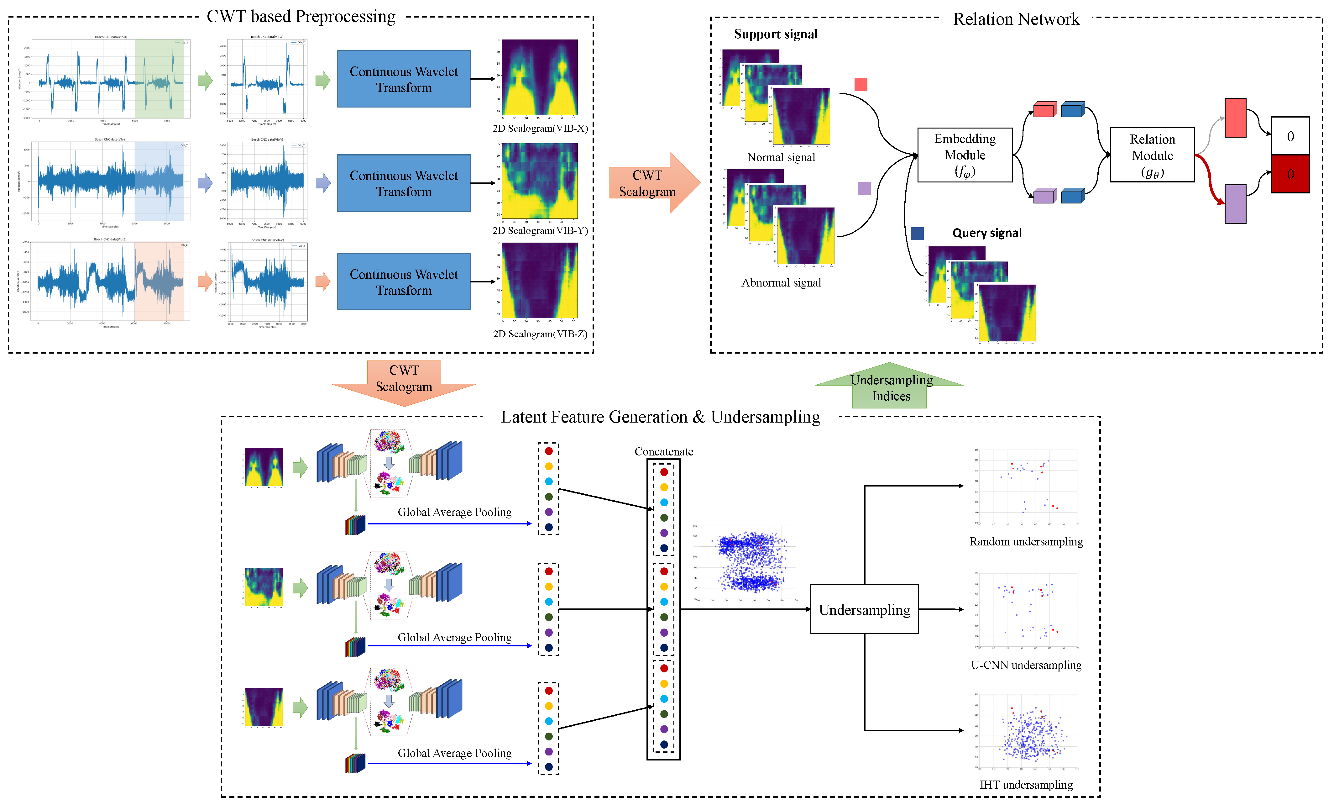
Figure 1. The overall architecture of the proposed fault diagnosis framework, illustrating the three stages: CWT-based preprocessing, Undersampling, and Relation Network classification.
Electronics 14 03699 g001
Figure 2. The architecture of the Relation Network for the diagnosis task. The Embedding Module extracts features, and the Relation Module calculates similarity scores (a learned metric) between the query sample and the support samples of each class.
Electronics 14 03699 g002
Figure 3. The structure of a confusion matrix for a binary classification task, where the positive class corresponds to the fault state. The components TP, TN, FP, and FN are used to calculate key performance metrics.
Electronics 14 03699 g003
Figure 4. Visualization of training data distributions. (a) Original imbalanced data. (b) After Random Undersampling. (c) After IHT Undersampling. (d) After U-CNN Undersampling, showing the preservation of critical boundary samples.
Electronics 14 03699 g004
Figure 5. Performance distribution of the SVM model across different undersampling strategies.
Electronics 14 03699 g005
Figure 6. Performance distribution of the VGGNet model across different undersampling strategies.
Electronics 14 03699 g006
Figure 7. Performance distribution of the proposed UnderFSL model across different undersampling strategies.
Electronics 14 03699 g007
Figure 8. Comparison of the best-performing models across all metrics. The box plots clearly demonstrate the superiority and stability (narrow IQR) of the proposed UnderFSL(U-CNN) framework.
Electronics 14 03699 g008
Figure 9. Visual analysis of the best model (UnderFSL with U-CNN). (a) The t-SNE visualization shows a clear separation between OK and NOK classes, demonstrating a discriminative learned feature space. (b) The confusion matrix confirms the model’s high recall and perfect precision over 10 episodes.
Electronics 14 03699 g009
Table 1. Detailed architecture of the relation network.
ModuleLayer/BlockConfigurationOutput Shape
Embedding
Module ( f ϕ )
InputCWT Scalogram (3 channels)64 × 64 × 3
Block 1Conv(3 × 3, 64), BN, ReLU, MaxPool(2 × 2)32 × 32 × 64
Block 2Conv(3 × 3, 64), BN, ReLU, MaxPool(2 × 2)16 × 16 × 64
Block 3Conv(3 × 3, 64), BN, ReLU, MaxPool(2 × 2)8 × 8 × 64
Block 4Conv(3 × 3, 64), BN, ReLU, MaxPool(2 × 2)4 × 4 × 64
Relation
Module ( g φ )
InputConcatenated Features (Block 4 × 2)4 × 4 × 128
Block 5Conv(3 × 3, 64), BN, ReLU, MaxPool(2 × 2)2 × 2 × 64
Block 6Conv(3 × 3, 64), BN, ReLU, MaxPool(2 × 2)1 × 1 × 64
Flatten-64
FC 18 nodes, ReLU8
FC 2 (Output)1 node, Sigmoid1
BN: Batch Normalization, FC: Fully Connected.
Table 2. Performance comparison of the proposed model and baseline methods on the Bosch CNC dataset (cross-machine validation). Best results are highlighted in bold.
ModelUndersamplingAccuracyRecallPrecisionF1-Score
SVMNone 0.52 ± 0.01 0.04 ± 0.02 0.54 ± 0.25 0.07 ± 0.03
Random 0.51 ± 0.02 0.03 ± 0.02 0.54 ± 0.24 0.06 ± 0.03
IHT 0.37 ± 0.12 0.41 ± 0.07 0.43 ± 0.12 0.41 ± 0.08
U-CNN 0.54 ± 0.04 0.15 ± 0.06 0.53 ± 0.19 0.24 ± 0.09
StatAENone 0.76 ± 0.02 1.00 ± 0.00 0.67 ± 0.01 0.80 ± 0.01
VGGNetNone 0.75 ± 0.17 0.51 ± 0.35 0.80 ± 0.40 0.59 ± 0.39
Random 0.61 ± 0.14 0.22 ± 0.28 0.5 ± 0.5 0.29 ± 0.34
U-CNN 0.61 ± 0.10 0.22 ± 0.19 0.7 ± 0.46 0.32 ± 0.26
IHT 0.34 ± 0.02 0.58 ± 0.04 0.39 ± 0.01 0.47 ± 0.01
UnderFSLNone 0.73 ± 0.13 0.47 ± 0.26 1.00 ± 0.00 0.59 ± 0.27
Random 0.84 ± 0.03 0.68 ± 0.08 1.00 ± 0.00 0.81 ± 0.05
IHT 0.69 ± 0.09 0.37 ± 0.18 1.00 ± 0.00 0.52 ± 0.19
U-CNN 0.96 ± 0.04 0.92 ± 0.08 1.00 ± 0.00 0.96 ± 0.05
Disclaimer/Publisher’s Note: The statements, opinions and data contained in all publications are solely those of the individual author(s) and contributor(s) and not of MDPI and/or the editor(s). MDPI and/or the editor(s) disclaim responsibility for any injury to people or property resulting from any ideas, methods, instructions or products referred to in the content.