Article

Decision Tree Pruning with Privacy-Preserving Strategies

1
Faculty of Information Science and Technology, Multimedia University, Jalan Ayer Keroh Lama, Melaka 75450, Malaysia
2
Centre for Advanced Analytics (CAA), COE for Artificial Intelligence, Multimedia University, Jalan Ayer Keroh Lama, Melaka 75450, Malaysia
*
Authors to whom correspondence should be addressed.
Electronics 2025, 14(15), 3139; https://doi.org/10.3390/electronics14153139
Submission received: 2 July 2025 / Revised: 1 August 2025 / Accepted: 4 August 2025 / Published: 6 August 2025

Abstract

Machine learning techniques, particularly decision trees, have been extensively utilized in Network-based Intrusion Detection Systems (NIDSs) due to their transparent, rule-based structures that enable straightforward interpretation. However, this transparency presents privacy risks, as decision trees may inadvertently expose sensitive information such as network configurations or IP addresses. In our previous work, we introduced a sensitive pruning-based decision tree to mitigate these risks within a limited dataset and basic pruning framework. In this extended study, three privacy-preserving pruning strategies are proposed: standard sensitive pruning, which conceals specific sensitive attribute values; optimistic sensitive pruning, which further simplifies the decision tree when the sensitive splits are minimal; and pessimistic sensitive pruning, which aggressively removes entire subtrees to maximize privacy protection. The methods are implemented using the J48 (Weka C4.5 package) decision tree algorithm and are rigorously validated across three full-scale NIDS datasets: GureKDDCup, UNSW-NB15, and CIDDS-001. To ensure a realistic evaluation of time-dependent intrusion patterns, a rolling-origin resampling scheme is employed in place of conventional cross-validation. Additionally, IP address truncation and port bilateral classification are incorporated to further enhance privacy preservation. Experimental results demonstrate that the proposed pruning strategies effectively reduce the exposure of sensitive information, significantly simplify decision tree structures, and incur only minimal reductions in classification accuracy. These findings reaffirm that privacy protection can be successfully integrated into decision tree models without severely compromising detection performance. To further support the proposed pruning strategies, this study also includes a comprehensive review of decision tree post-pruning techniques.

1. Introduction

In data classification, machine learning algorithms have been successfully applied to resolve many predictive tasks in various domains. By providing sets of instances (dataset) to a machine classifier, it is able to learn the importance of each bit of data according to the heuristics underneath a classifier and subsequently gain the ability to predict new instances. The field of privacy began to gain huge attention in recent years due to the explosion of artificial intelligence and the advancement of data storage technology. Privacy concerns have led the statistical research communities to propose a distinct set of data privacy algorithms for concealing the sensitive information found in the dataset (privacy-preserving data publishing [1,2]). On the other side of the coin, researchers have also fine-tuned many machine learning algorithms to consider the importance of privacy (privacy-preserving machine learning [3,4,5]).
Privacy-preserving data publishing intends to safeguard the privacy of data by sanitizing or anonymizing the information before performing any classification tasks, while privacy-preserving machine learning aims to prevent sensitive information from being inferred by the machine learning models. Unlike most of the works proposed, we have utilized the decision tree pruning approach for concealing the sensitive values appearing in the decision tree model by removing the particular nodes containing the sensitive data.
A white box model, the decision tree, is selected in this paper because of its ability to generate straightforward, simple, and understandable classification rules. Although the tree model is able to perform at a satisfactory level in various domains, it is also susceptible to various privacy issues. As the model of a tree classifier provides the class distributions of each node, Li et al. [6] describe the possibility of deidentification for a particular individual by illustrating the scenario using a decision tree model. Unlike the privacy pruning designed by Li et al. [6], our approach focuses on the splitting values of a decision tree model. From a fully built decision tree model, the proposed pruning approach will remove the particular nodes whenever a predetermined sensitive value is detected on each iteration of the pruning procedure. The merit of this approach is the unaltered decision tree induction for generating the tree model. In other words, the entire procedure for inducing the tree follows the original statistical heuristics (e.g., information gain [7], information gain ratio [8], or Gini index [9]).
Our work is motivated by the application of decision trees on Network Intrusion Detection Systems (NIDSs), and the privacy concerns are described in Section 4. This study is an extended version of our previous work [10], where we initially proposed a sensitive pruning-based decision tree for privacy protection in Network-based Intrusion Detection Systems. The earlier work introduced the concept of pruning sensitive nodes to mitigate privacy risks associated with decision tree visibility. However, the prior study was limited to a single NIDS dataset (6% GureKDDCup) and employed only the standard sensitive pruning strategy. In this paper, we further develop and enhance the sensitive pruning framework by introducing two additional pruning strategies: optimistic and pessimistic sensitive pruning. Moreover, the current study significantly expands the experimental validation by testing on multiple large-scale NIDS datasets and integrating additional privacy-preserving techniques such as IP address truncation and port bilateral classification. The extended experiments, improved algorithms, and detailed complexity analysis provide a more comprehensive view of the practical applicability and scalability of the proposed approach in diverse NIDS environments. In this paper, the proposed privacy pruning approach is enhanced based on the C4.8 decision tree algorithm (better known as J48 in the Weka package).
Related work on post-pruning algorithms is reviewed in Section 2. Section 3 described our proposed privacy post-pruning in detail. Application and motivation of the designed algorithm are explained in Section 4. Section 5 provides the experimental settings and empirical results tested against three NIDS datasets. Lastly, Section 6 concludes our work along with some future works and challenges.

2. Related Works

The decision tree model often suffers from the dilemma of overfitting its training data due to its greedy approach employed in building the classifier. To resolve the issues of overfitting, the pruning approach was proposed to simplify an unpruned decision tree by removing the insignificant node or branch. Generally, pruning can be categorized into two groups, which are pre-pruning (forward pruning) and post-pruning (backward pruning).
Pre-pruning was designed in such a way that it stops the growth of the tree during the process of decision tree induction based on some statistical significance test. For example, the chi-squared test [7] would prohibit the growth of the tree when the attributes selected are not statistically significant. Although pre-pruning required lesser computational resources as compared to post-pruning, pre-pruning suffers from a few of the disadvantages: (i) premature tree (early stopping), (ii) threshold selection, and (iii) horizon effects phenomenon. The idea of premature trees has been explained very well in terms of the XOR problem [11]. Breiman [9] pointed out the difficulty in attaining the appropriate threshold, as a higher threshold will lead to extreme pruning that might destroy significant nodes or branches, and a lower threshold would result in only slight simplification. Horizon effects are reflected in a situation whereby the descendants of the current nodes are pruned even though it does not fulfill the pruning condition [12,13]. This is because the nature of the pre-pruning procedure will not examine the child of the pruned nodes, as the nodes do not exist in this case.
Post-pruning was introduced to complement the disadvantages of pre-pruning in exchange for higher computational complexity. Post-pruning first allows the decision tree model to overfit (unpruned) the training data; then some heuristics are utilized for removing the unreliable nodes or branches. In general, most post-pruning algorithms adopt the bottom–up transversal strategy whereby the pruning criteria will be evaluated from the bottom of the tree (leaves) towards the top of the tree (root). Additionally, the node or subtree can only be pruned if all of its descendants conform to the pruning evaluation criteria [14,15]. This constraint has been introduced to avoid the horizon effects as described in pre-pruning. As computational cost is no longer a substantial predicament for this era, researchers have proposed various new post-pruning techniques with the objective of achieving better trees in terms of classification accuracy and generalization. Although there are several pieces of literature reviewing the distinct type of pruning techniques, most of the reviews are decades old and outdated [12,15,16]. An updated survey [17] on decision trees recently examined advances in fitting, generalization, and interpretability; however, pruning was addressed only briefly, leaving room for deeper exploration of this topic. More recently, a comprehensive review [18] focusing on the mathematical fundamentals of decision tree pruning was published, emphasizing algorithmic strategies and computational complexity. In contrast, this paper presents a thorough review that covers the majority of pruning techniques, integrating both classical and more recent approaches. From this section onwards, the term pruning refers to post-pruning unless mentioned.

2.1. Pruning-Based Misclassification Error Rate (Minimum Error)

As classification accuracy is an essential performance evaluation criterion, the majority of enhancement and modification of algorithms tends to focus on improving the accuracy of classifiers. This similar objective does not exclude the pruning procedure, as a lot of work has been conducted on the pruning algorithms in order to improve the classification accuracy or minimize the classification error.
Quinlan et al. [14] propose a method, Reduced Error Pruning (REP), by assessing the error rate based on a new validation set before and after replacing an internal node with its most frequent class. If the error rate of the pruned tree is lower than the unpruned tree, the pruned version will be kept, and subsequent pruning will occur for each internal node until there is no gain in accuracy across the validation set. As REP follows a bottom–up approach, an internal node can only be pruned if all of its subtrees for the selected internal node do not improve the overall accuracy of the tree.
At the same time, Quinlan et al. [14] also introduced Pessimistic Error Pruning (PEP), which utilizes the statistical properties of continuity correction for binomial distribution. A constant of 0.5 classification error is added to every node in an attempt to obtain a much more realistic error rate in comparison to the optimistic error rate calculated solely based on the same training set, which is adopted for growing and pruning the tree. Additionally, one standard error rate is also proposed to be added on top of the adjusted classification error for a subtree. In other words, a subtree will only be pruned if the adjusted error rate for the pruned node is lower than the adjusted error rate plus one standard error for the subtree under the selected pruned node. Unlike REP, PEP does not require a separate validation set for calculating the error rate. Contrarily, PEP follows a top–down traversal strategy that prioritizes pruning a tree before considering its subtree. Similar to the pre-pruning procedure, PEP also suffers from the horizon effects due to its top–down pruning approach. In practice, PEP is faster compared to a bottom–up approach, as the children of the pruned nodes are not required to go through the error estimation in the pruning process.
To further reduce the optimistic bias in training data, error-based pruning (EBP), the improved version of PEP, is adopted in the popular C4.5 decision tree induction developed by Quinlan et al. [8]. In contrast to PEP, EBP measures the error rate in a much more pessimistic estimation by utilizing the upper limit of confidence intervals. Apart from the standard node pruning (subtree replacement), EBP also permits the popular branch to be replaced by the subtree or nodes (subtree raising/subtree grafting [19]) if it conforms to the lowest error rate. EBP compares three types of error rate: (i) error on subtrees (unpruned), (ii) error after replacing the node with a leaf node, and (iii) error after replacing the node with the largest branch. Based on the lowest error attained, the node can either be (i) unaffected, (ii) replaced with a leaf node, or (iii) replaced with the largest branch. Similarly, EBP follows a bottom–up approach, like REP. Although the statistical properties employed in both PEP and EBP seem to be statistically invalid [13,16,20], experimental results have shown the competency of adopting the statistical theory for improving the performance of a decision tree. All of the three pruning methods proposed by Quinlan et al. [8,14] aim to solve the problem of overfitting from the perspective of classification error.
Mingers [15] proposed a method, Critical Value Pruning (CVP), by exploiting the decision tree induction splitting criterion (e.g., information gain and gain ratio) and introducing a fixed threshold as a metric for the pruning procedure. In CVP, a node will be pruned if the value of the splitting criterion is smaller than the fixed threshold. The author claims that the splitting criterion represents the strength and importance of a node and is thus suitable to be adopted because the metrics express the correlation between the class and splitting attribute value at the specific node. The essential drawback from this method is the necessity of a domain expert for selecting the most optimum threshold. Furthermore, Jensen et al. [21] pointed out that identical probabilities adopted during training and pruning are flawed. As a similar metric is utilized, it would definitely result in highly biased probabilities [21].
Concurrently, Mingers [15] also proposed a method, Minimum Error Pruning (MEP), based on Laplace error estimation for adjusting the error rate by employing the training dataset [13]. MEP estimates the errors of each node by assuming the entire distribution in the node follows the majority instances class. Unlike the methods proposed by Quinlan et al. [8,14], Mingers includes the number of classes in the estimated error rates. Similar to most classification error-based pruning, MEP adopts the similar bottom–up traversal strategy, and pruning will only occur if and only if the estimated error rates when replacing the nodes with a leaf are smaller compared to the unpruned tree. An improved version of MEP was then devised by Cestnik and Bratko [22] to solve the issues of optimistic bias [23] and the dependency of the estimated error rate based on the number of classes [15]. Cestnik and Bratko modified the original Laplace heuristics introduced by Mingers. Instead of relying on the number of classes, the authors introduced the usage of class prior probability as well as a constant that controls the severity of pruning. To obtain the optimum value of the constant, they suggested tuning the constant with a validation set if the dataset available is large enough; otherwise, a cross-validation approach can be adopted in exchange for a higher computational complexity.
Zhang et al. [24] establish a new variant of MEP, Improved Expected Error Pruning (IEEP). In consideration towards the missing attributes, the proposed algorithm will expand the branch with the splitting attribute equivalent to ‘unknown node’ when missing attributes, which are denoted as ‘?’, are chosen. In addition to the error estimation adopted in the previous works [15,22], the authors complement a third error estimation by dividing the total number of unknown nodes by the total number of leaf nodes. The obtained error estimation is then compared with a predetermined threshold value, which is equal to 1/3. If the error estimation is lower than the threshold, the node will be pruned accordingly. However, the selection of the threshold value is not explained by the authors.
Mitu et al. [25] proposed a pruning-based ensemble method for multi-class classification, where an individual decision tree is created for each feature. Post-pruning is applied to each tree, and the best tree is selected based on cost–complexity criteria. These selected trees are then combined into an ensemble, with predictions determined through majority voting. Their approach outperformed the standard C4.5 algorithm on several UCI Machine Learning Repository datasets, including Wine, Breast Cancer, Iris, Titanic, Heart, and Lung, achieving accuracy improvements of up to 11% on some datasets.

2.2. Pruning-Based Structural Complexity

A decision tree is a white-box model that generates a sequence of simple rules that can be easily studied, analyzed, and interpreted. Although minimizing the classification errors is a unanimous goal for most classification models, having a complex structure of decision trees by prioritizing the accuracy would destroy the sole purpose of a decision tree. Thus, if a simpler structure of a decision tree is able to be attained by sacrificing negligible accuracy, the simpler structure should be preferred.
The first post-pruning algorithm was originally proposed by Breiman et al. [9] in Classification and Regression Trees (CARTs). The published method, Cost–Complexity Pruning (CCP), considered the importance of both the misclassification rate and complexity of the tree. The tree complexity in this case is measured based on the total number of leaves. Two stages are involved in the procedure of CCP. First, once a fully grown tree has been induced by the CART, CCP is directly applied to every node by using a bottom–up traversal strategy for generating a sequence of pruned trees. The smallest subtrees are formed based on each of the leaves from a fully grown tree. Starting from the leaves towards its antecedent (parent), each iteration towards the root will subsequently generate a new subtree. In contrast to most pruning algorithms, each selected candidate for CCP is required to consider all of its internal nodes (child/descendant). Second, to select the best tree among the sequence of trees generated, a validation set is essential for examining the classification error because training sets, which have been utilized for growing the tree, are not suitable, as they will definitely favor the unpruned version of the tree. The best tree is then selected based on the lowest classification error resulting from the validation set. The cross-validation approach can also be adopted in a situation of insufficient training data. Although CCP takes into account both the error and the structural complexity of a tree, generation of the sequence of trees would yield a computational complexity higher than most pruning algorithms because it is necessary for each pruning candidate to consider all of its descendants [16]. To achieve the optimum size of tree, Gelfand et al. [26] improved the original algorithm by suggesting the full training datasets be divided into two subsets, whereby each subset contains half of the training data. The first subset is then utilized for growing the tree, while the second subset is employed as the validation (pruning) set. Iteratively, the growing and validation sets can be swapped during each iteration. Authors reported that the enhanced algorithm performs faster and more accurately in comparison to the original algorithm.
Bohanec and Bratko [27] defined an optimal pruned tree as the smallest pruned tree with respect to the number of leaves (size) that results in the lowest classification error (highest accuracy). The first variant of the optimal pruned tree was designed by Breiman et al. [9] in the CART algorithm. However, Bohenec and Bratko [27] point out that Breiman et al.’s approach is computationally infeasible because the number of subtrees generated increases, respectively, with the size of the tree. To design an efficient Optimal Pruning Algorithm (OPT), the authors adopted dynamic programming for solving the problem in an efficient polynomial time. In contrast to CCP, which evaluates the importance of a subtree based on the weighted classification error and number of leaves, OPT seeks to search for the lowest classification error of a pruned tree by comparing the error rate of all possible combinations of subtrees with respect to the number of leaves (size) of the recommended pruned tree. Similar to most pruning algorithms, OPT uses the standard bottom–up approach in their pruning strategy. Additionally, OPT utilizes the same training data for estimating the error rate of each node. In their work, they assume the absence of noise from their training data, subsequently leading the classification error for the unpruned tree to always be equivalent to zero. A total of the original number of leaves minus one sequence of the optimal tree will be generated by using OPT, each sequence yielding the best tree (lowest error) with respect to the number of leaves. Although the OPT employed is quite similar to CVP, Bohenec and Bratko [27] mention that CVP might not always be able to attain the smallest tree with the lowest classification error. To reduce the computation complexity of OPT, Almuallim [28] proposed an enhanced variant of OPT based on the initial OPT designed by Bohenec and Bratko [27].
Lazebnik and Bunimovich-Mendrazitsky [29] designed a post-pruning algorithm based on Boolean satisfiability (SAT-PP), which was evaluated on several clinical datasets, including breast cancer, lung cancer, and cervical cancer datasets. Their method effectively reduced decision tree size while preserving classification accuracy and achieved a reported 6.8% reduction in computation time compared to standard pruning approaches. Bagriacik and Otero [30] proposed a fairness-guided pruning method for decision trees aimed at enhancing interpretability. Their approach integrates fairness metrics into the post-pruning process by replacing sub-trees with the most common branch or leaf. Experimental results demonstrated improved fairness and simplified tree structures, with only a minor reduction in model performance.

2.3. Pruning-Based Multiple Metrics

In general, most pruning algorithms are designed with the intention of solving a single objective problem, e.g., classification accuracy or structural complexity. However, Muata and Bryson pointed out that [31] other performance measures, such as the stability and interpretability of a decision tree model, are also crucial evaluation criteria for gauging the quality of a decision tree.
Fournier and Cremilleux [32] proposed Depth–Impurity (DI) pruning that is built upon a quality index, Impurity Quality Node (IQN). IQN measures the quality of a node based on the impurity and depth of a node. Barrientos and Sainz [33] defined impurity as the “average distance of all the data belonging to a leaf node to its center of mass”. Authors claim that DI pruning does not rely on the misclassification error rate adopted in most typical post-pruning algorithms, and it does not proceed to remove a subtree when the classification error rate of the subtree is equivalent to its antecedent. This is because the author’s intention is to solve the issues in uncertain domains; the larger trees containing the extra leaves are preferred in this case. Although most pruning algorithms would prefer a simpler (smaller) tree when the classification accuracy of a subtree is equal to its antecedent, Muata and Bryson [31] disclosed that different decision tree problems might have a distinct evaluation for the simplicity (number of leaves) of a tree.
Wei et al. [34] reveal that the complexity of a tree should not include only the number of leaves as described in CCP; they propose to consider both the level of the tree as well as the accuracy of each selected pruned node by utilizing rough set theory [35]. The method was extended by the same author [36], and the structural complexities of a tree were evaluated based on the combination of (i) number of leaf nodes, (ii) number of internal nodes, (iii) level of the tree depth, (iv) number of classes (label), and (v) number of conditional attributes involved in the subtree. The experimental results involving 20 benchmark datasets show that a smaller tree size with similar accuracy is able to be attained by using the proposed pruning algorithm as compared to C4.5 with REP. Similar to OPT [27], Wei et al.’s [36] pruning algorithm employed the training set for evaluating the classification error and follows the standard bottom–up pruning fashion.
Muata and Bryson [31] designed a multi-objective evaluation criterion by using mixed integer programming formulation. From their work, they evaluated the performance measures based on the four categories: (i) classification accuracy, (ii) simplicity of decision tree, (iii) stability of decision tree, and (iv) discriminatory power of leaves. Although the pruning algorithm has been successfully modified to consider multiple performance measures and has demonstrated its capability in the Abalone dataset, the proposed method suffers from a high computational complexity and might not be suitable for adoption in the case of a huge number of nodes. The same authors also integrated the proposed evaluation criteria in conjunction with post-pruning for the regression tree in [37].
Based on the similar concepts, Wang and Chen [38] proposed a multi-strategy pruning with the use of a performance parameter that is obtainable based on the three metrics: (i) total number of instances for training and testing data, (ii) classification accuracy, and (iii) scale of the tree, which includes the depth and number of leaf nodes. They reported that the algorithm suggested is able to achieve a lower error rate as compared to a standard C4.5 when tested against an Intrusion Detection System dataset, KDD’ 99.

2.4. Pruning with Weighting (Cost-Sensitive)

Most pruning strategies discussed in the previous sections treat all of the classes in the dataset as equally significant. However, this is not always true for a real-world classification problem because a certain error (mistake) might be severe compared to another. For example, approving a loan to a questionable individual might be much more expensive in contrast to rejecting a loan to a reliable individual. Other examples include the misclassification in the scenarios of disease (cancer) diagnosis [39].
To tackle the issues of unequal misclassification costs, Knoll et al. [39] proposed the first method, Cost-Sensitive Pruning (CSP), by introducing weights (misclassification costs) for each class in the dataset. Although the experimental results suggest some improvement in terms of accuracy, Knoll et al. [39] remark that the outcome of the classification heavily relies on the cost matrix associated with each class. Since their work is much concerned regarding the applicability of the misclassification costs across various pruning algorithms, the value of the cost matrix is supplied directly by the author and is not discussed in depth.
Bradley and Lovell [40] adopted the Receiver Operating Characteristics (ROC) curve for discovering the most suitable ratio of misclassification costs. Instead of weighting the misclassification in accordance with each class [39], the authors suggest weighting the costs based on the two types of misclassification: (i) false negatives and (ii) false positives. To find the best ratio between the two misclassification costs, a trial-and-error approach by weighting the ratio with several values is assessed with the pruning algorithms, and the results obtained are subsequently plotted onto an ROC curve. In their work, they claim that the ROC approach employed is able to furnish the decision tree pruning with flexibility in tuning the number of instances that fall under the category of false negatives and false positives.
Ting [41] introduced instance-weighting into the C4.5 decision tree for inducing a cost-sensitive tree classification. Unlike the cost matrix proposed by Knoll et al. [39] in CSP that required to be manually selected, Ting calculated the cost matrix associated with each class by summing up the total misclassified instances according to each class from the full training samples. It is necessary for the weight of each class to be recomputed at each node, and the weight of a class is proportional to the misclassifying cost and dependent on the number of instances associated with each class at the particular node. The method is proposed to enhance the C4.5 decision tree induction; however, in terms of pruning, the pruning process adopted the weight of the class instead of the number of misclassified instances for the selected pruning candidate. As the cost matrix is derived directly from the full training samples, the proposed method may not be able to perform well in an unbalanced class distribution scenario.
Bradford et al. [42] extend the original CCP [9] by incorporating a cost matrix along with Laplace Correction to minimize the loss. Several experiments have been conducted by the authors by integrating the Laplace Correction with other pruning algorithms (e.g., C4.5 and Kullback–Leibler (KL) pruning). Authors reported that the application of Laplace Correction is beneficial to all of the pruning algorithms. However, the comparison of experimental results is limited because not all of the pruning algorithms adopted the cost matrix; only CCP included the cost matrix.

2.5. Hybrid Pruning

Hybrid algorithms refer to a combination of classifiers integrated for the purpose of improving the performance of an original classifier. In pruning, several algorithms have been integrated with pruning for enhancing its performance.
Chen et al. [43] integrate a genetic algorithm into the post-pruning process to resolve the issues of overfitting. They encoded the decision tree model with a sequence of 0 and 1 to fit the hypothesis of the genetic algorithm, where 0 represents the connected edge and 1 represents the disconnected (pruned) edge. Then, the sequence is utilized for optimizing the weights in the fitness function. Subsequently, crossover and mutation operators can then take place to produce new offspring. The authors reported that the genetic pruning algorithm performs equally with other pruning methods. However, the experimental results only compared the unpruned decision tree against the proposed method.
Zhang and Li [44] proposed to apply Bayesian theory directly on a fully built C4.5 decision tree as a pruning criterion. In the post-pruning process, nodes are pruned if they did not satisfy the two verification strategies in Bayesian theory, which are necessity verification and sufficiency verification. The authors claim that the Bayesian pruning procedure is able to produce smaller trees, improved efficiency, and higher prediction accuracy when tested against the Beijing University internal datasets. In 2015, Mehta and Shukla [45] incorporate the same Bayesian pruning strategies into the C5.0 algorithm. Tested against patient’s data (not mentioned which dataset), the authors reported an improvement in terms of tree size, accuracy, and memory consumption.
Malik and Arif [46] designed a pruning algorithm based on the concept of Particle Swarm Optimization (PSO). Two variations of PSO are proposed by the authors, which are the single-objective PSO pruning algorithm and the multi-objective PSO pruning algorithm. Single-objective PSO refers to optimizing the true positive rate, while multi-objective seeks to optimize both the true positive rate and the false positive rate. Instead of following the standard bottom–up or top–down traversal strategy of pruning, the proposed PSO arbitrarily selects a group of nodes to be retained or pruned according to its heuristics. Tested against the KDDCup 99′ Intrusion Detection dataset, the authors reported an improvement of performance in terms of tree size, false positive rate, and true positive rate. However, it is not appropriate to adopt the testing set for fine-tuning the PSO parameter value, as it would subsequently result in a biased model.
Sim et al. [47] proposed an Adaptive Apriori (AA) boosted decision tree model, Boosted Adaptive Apriori post-pruned Decision Tree (AAoP-DT)s. Before generating the decision tree model, AA properties are employed for assessing the traits of the datasets for determining the number of depths required for decision tree induction. Utilizing the similar AA properties for reducing the complexity parameters in post-pruning, the authors claim that a better optimized tree can be produced. The authors also integrated similar AA properties for the pre-pruning procedure in [47].
Ahmed et al. [48] employed Bayes Minimum Risk (BMR) as a pruning evaluation criterion. Originally, BMR was proposed by Bahnsen et al. [49] for balancing the trade-offs between legitimate class transactions and fraud class transactions in credit card fraud detection. Associating BMR along with the cost matrix of each class for measuring the risk, the experimental results claim the integration is able to improve the performance of fraud detection. In pruning, Ahmed et al. [48] adopted the similar BMR for comparing the risk before and after pruning a node instead of utilizing the classic misclassification error. A node will be pruned by BMR if the risk of the parent node is lower than its weighted risk of children. The proposed BMR pruning is able to achieve better accuracy and similar structural complexity in contrast to REP and MEP when tested with five different datasets.

2.6. Other Pruning

Apart from the mainstream pruning algorithms discussed, some of the less well-known pruning techniques that intend to improve pruning from a different perspective are worth mentioning.
Statistical significance tests. Jensen and Schmill [21] use Bonferroni correction for tuning the significance levels of multiple statistical tests. Authors reported that a smaller tree is obtained from their experimental results. Pruning with significance tests has also been widely explored and experimented with by Frank and Witten [13]. They adopted REP in conjunction with statistical significance tests for producing a better pruned tree. Experimental results presented show that a much more accurate and smaller tree can be attained given that suitable significance levels are predefined by a domain expert. In order to complement the needs of a domain expert, the authors also proposed to use validation sets or cross validation for determining the optimum significance levels. Several other statistical test-related techniques are also explored in [11,50]. Another line of research closely related to statistics investigates the application of 0.632 bootstrap resampling in error estimation to replace the standard cross-validation [51,52].
Penalty terms. CCP [9] in the literature commonly follows the standard additive penalties. Generally, this is because a faster, more efficient, and easier pruning algorithm can be implemented. However, Coull [53] argued that theoretically, adoption of subadditive penalties should perform better than the standard additive penalties. In contrast to the additive penalties that escalate linearly as the size of the decision tree increases, subadditive penalties increase with the square root of the size of the decision tree. Although both of the penalty terms increase as the size of the decision tree increases, subadditive (square root) penalties are much slower compared to additive penalties. Although the concepts of subadditive penalties are mathematically proven by Scott [53], experiments incorporating CART with subadditive penalties are empirically compared against the additive penalties in [54]. From the experimental results, Garcia-Moratilla et al. [54] reveal that no significant improvements in terms of generalization and classification are observed when subadditive penalties are utilized.
Minimum description length (MDL). Complexity or cost of a model can be evaluated by the number of bits required to generate a model through the MDL principle [55]. The complexity of a model in this case is strongly affected by the coding scheme. In terms of pruning, Mehta et al. [56] have successfully adopted the MDL principle for pruning a decision tree. A smaller tree is observed in the experimental results when compared against PEP and EBP. Authors also reported that a similar error rate is obtained for each of the pruning algorithms.

2.7. Privacy Pruning

Classification attacks, or re-identification attacks by linking information, have been described by Sweeney [57]. The author claims that an individual is highly possible to be uniquely identified based on the three following pieces of information: (i) ZIP code, (ii) gender, and (iii) date of birth. To illustrate the attacks, Sweeney links patient data and voting data by intersecting both of the datasets according to the three aforementioned pieces of attribute information. Based on the similar concepts, Li and Sarkar [6] mentioned that the properties of a decision tree that splits the training data into smaller groups based on information gain heuristics further escalate the risk of disclosure. This is because a decision tree will tend to split its training data until it is able to achieve a pure leaf node, attaining 100% training classification accuracy. As the final leaf node consists of a very small size of training data, e.g., only two male individuals over the age of 78, Asian, and with the zip code of 10001. Linking the relevant information obtained from an unpruned decision tree with a publicly available source makes it possible to reveal the identity of an individual and the confidential attribute values. On the other hand, authors also described the suitability of decision trees to be utilized as personal information mining tools. This can be achieved by altering the original class (label) to the private (confidential) attribute. By doing so, the decision tree generated will try to predict the private (confidential) or missing values based on the testing data supplied.
To resolve the complication, Li and Sarkar [6] proposed a new entropy-based pruning evaluation for measuring the disclosure risks of each node. On an unpruned tree, a node will be pruned if the disclosure risk assessment is higher than a pre-specified threshold provided. A smaller and purer node will result in a higher risk of disclosure as compared to a bigger and impure node. In contrast to the typical pruning procedures such as CCP and EBP, which aim to minimize the classification error by removing the insignificant nodes, the proposed pruning algorithm operates differently, as it monitors the amount of data available for data swapping during the pruning process for decreasing the disclosure risks. Once the pre-set disclosure risk threshold has been achieved, each leaf of the final tree will undergo the data swapping procedure. In a two-class (binary) problem, the majority class records are swapped with the minority class records within the same leaf randomly while still retaining the final probability of majority class records being superior to the minority class records. One of the drawbacks of the approach proposed is the necessity of a domain expert for determining the initial disclosure risk measures that control the severity of pruning and data swapping. In contrast to the existing statistical anonymization techniques, the proposed method can be adopted to safeguard the privacy of both numeric and categorical data without the need of conversion or translation of data.
Even though the pruning algorithm [6] is designed to solve the privacy issues from the perspective of a decision tree, the method employed and scenarios considered are entirely different from the pruning algorithm we proposed in this paper. The main objective of Li and Sarkar’s [6] algorithm is to prevent classification attacks against the small distribution allocated at the lower level of the decision tree. By swapping the class labels for each leaf, an uncertainty is induced, subsequently leading to better protection against classification attacks. In our work, we consider the sensitivity of the attribute value instead of the data distribution.
From the recent study, it can be seen that most of the proposed pruning algorithms focus on improving the performance of a decision tree model in terms of accuracy or structural complexity. Furthermore, only one piece of literature has tried to tackle the issues of privacy from the decision tree pruning viewpoint. Thereafter, there is still further room for improving the pruning procedure to consider privacy concerns in the decision tree model.

Computational Complexity in Privacy Preservation

Decision tree size can be reduced either by restricting maximum depth or through pruning strategies. While most existing works focus on limiting tree depth, Pantoja et al. [58] approached privacy from a different perspective by minimizing private information leakage (e.g., religion or nationality) across the entire tree structure. Their method automatically evaluates each potential branching question during tree construction; if adding a branch would increase the probability of inferring a private attribute beyond a predefined threshold, that branch is discarded. This privacy-driven constraint naturally limits the tree’s growth, controlling its size and preserving privacy without explicitly enforcing a depth limit. Conceptually, this is similar to the probability-based node handling in Li and Sarkar’s [6] label-swapping method. However, instead of swapping the class labels, Pantoja et al. [58] focus on private attribute distributions and remove branches entirely when privacy risks exceed the predefined thresholds.
Regarding computational complexity, Patil et al. [59] proposed a multi-level pruned classifier applied to a credit card dataset containing 101,580 records. Their algorithm employed pre-pruning during tree construction, halting growth once a predefined pruning level was reached. By selecting only the most contributive attributes, the resulting trees contained fewer nodes and generated fewer rules than standard C4.5 and thus achieved lower classification time complexity and bandwidth usage while maintaining comparable predictive performance. Following a similar rationale, our proposed sensitive pruning strategies also report node counts and training/testing times to highlight computational efficiency relative to unpruned models.

3. Proposed Model

As depicted by Li and Sarkar [6], confidential information can be inferred from a fully built decision tree by linking attacks. In our studies, we proposed a distinct way to protect the sensitive information in a decision tree. The proposed pruning algorithm is extended from the original J48 (Weka C4.5 package) for considering the importance of privacy.

3.1. Sensitive Pruning

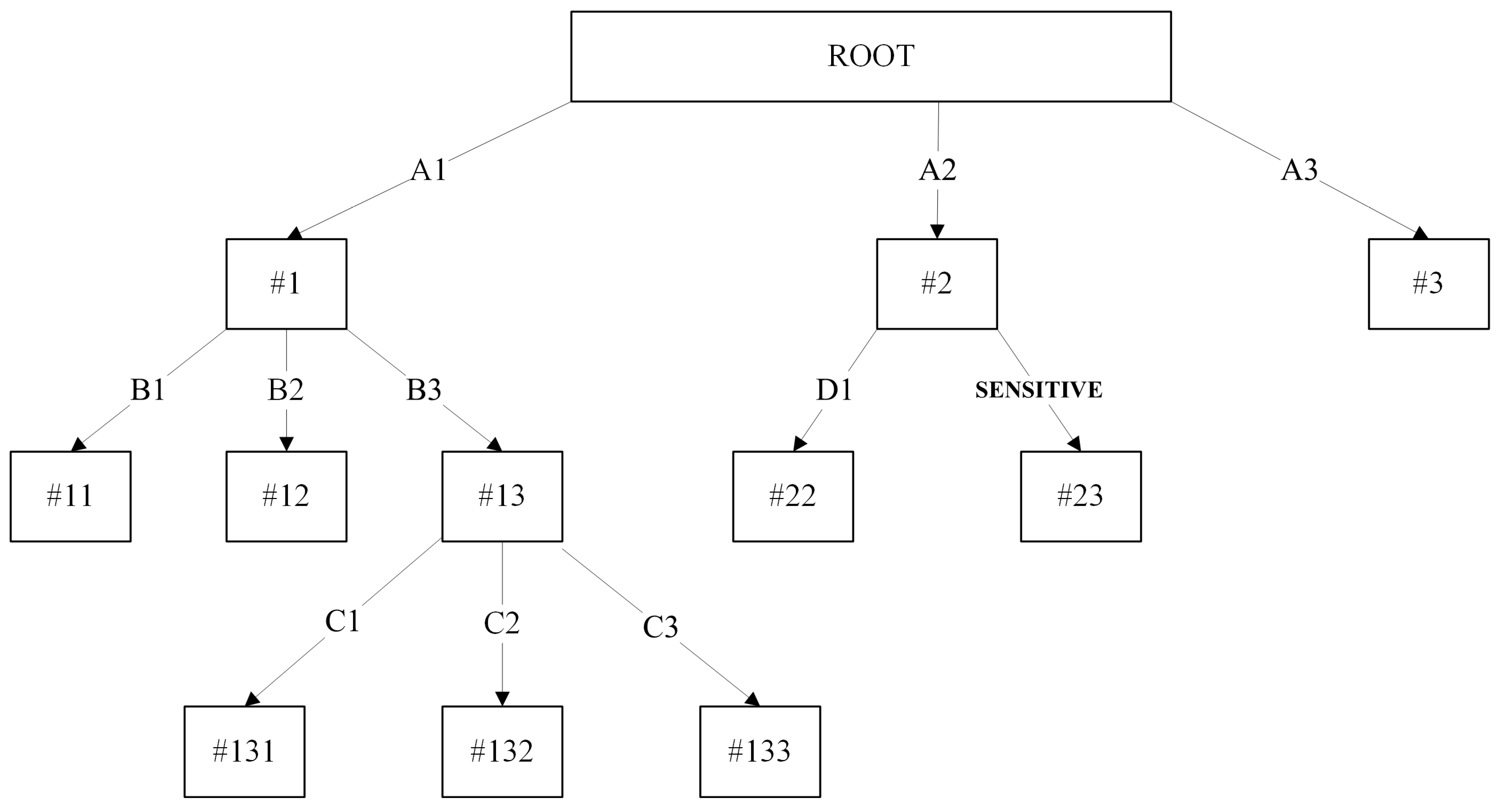
Figure 1 presents a simple unpruned decision tree. A decision tree starts from a root and splits by selecting the best attribute (e.g., A, B, C, and D) iteratively until it is able to achieve a pure leaf node. The splitting attribute value is represented as A1, A2, A3, B1, etc., while the nodes are represented by #1, #11, #12, #2, #3, etc.
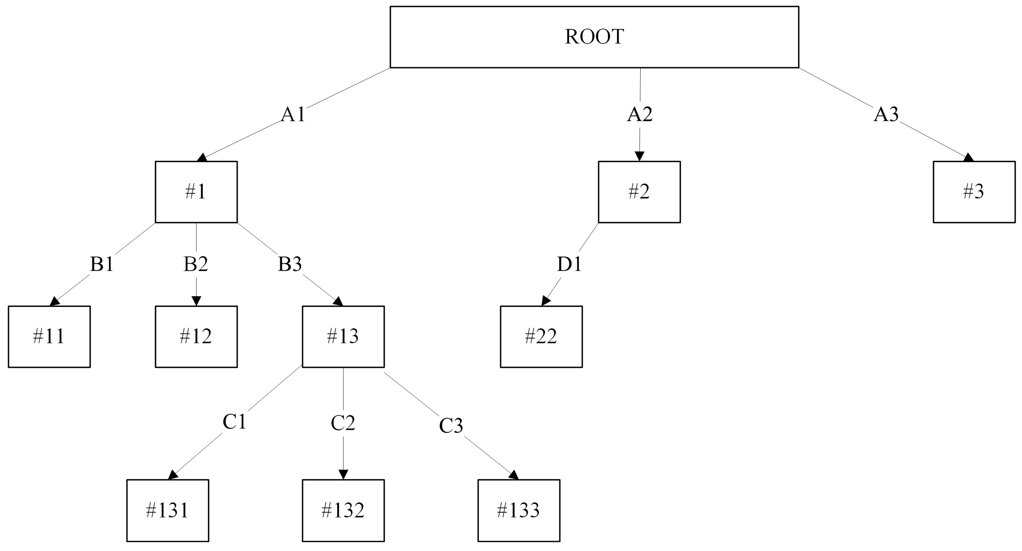
To illustrate the concepts of our proposed algorithm, let us assume that attribute value B3 is a confidential value. Following the standard bottom–up post-pruning strategy, our proposed method will compare each of the attribute values with the value of B3. If its value is equivalent to B3, we will prune the related node #13 to a leaf and modify the attribute value of B3 to “SENSITIVE”. Since node #13 consists of three children, #131, #132, and #133, all of its children will be removed as it is no longer significant in the classification process. Although node #13 is no longer useful in classification, the strength of the decision tree allows each of the nodes in the model to perform classification tasks. In this case, node #1 will handle the classification duty on behalf of node #13, as the testing instance is not able to traverse to the leaf of the decision tree. Additionally, retaining the sensitive node #13 might also give a better insight to the decision tree user. It is also worth mentioning that the removal of the class label for node #13 or even the entire node #13 can be performed without affecting the current classification ability of the entire model. Figure 2 shows the decision tree model after the sensitive pruning procedure.
The sensitive pruning algorithm can be summarized as follows in Algorithm 1:
Algorithm 1: Sensitive Pruning Algorithm
Input:
    Tmax, Unpruned Decision Tree
    Sensitive Attribute Value, AS
Output:
    Pruned Sensitive Decision Tree
Procedure:
Learning Procedure I:
1.  for all split in node t, do
2.      Let node ts be the child node of t
3.      Let Attribute Value A equals to current split attribute value
4.      if (A == AS):
5.       Replace A value with “SENSITIVE”
6.       if (ts contains any child node):
7.        Replace ts with a leave node
8.       endif
9.      endif
10.  Endfor
Learning Procedure II:
11. Let T = Tmax
12. if T is not “leave node”:
13.   for all node tT, starting from leaf nodes towards the root node, do
14.        Repeat step 1–10
15.   endfor
16. endif

3.2. Optimistic Sensitive Pruning

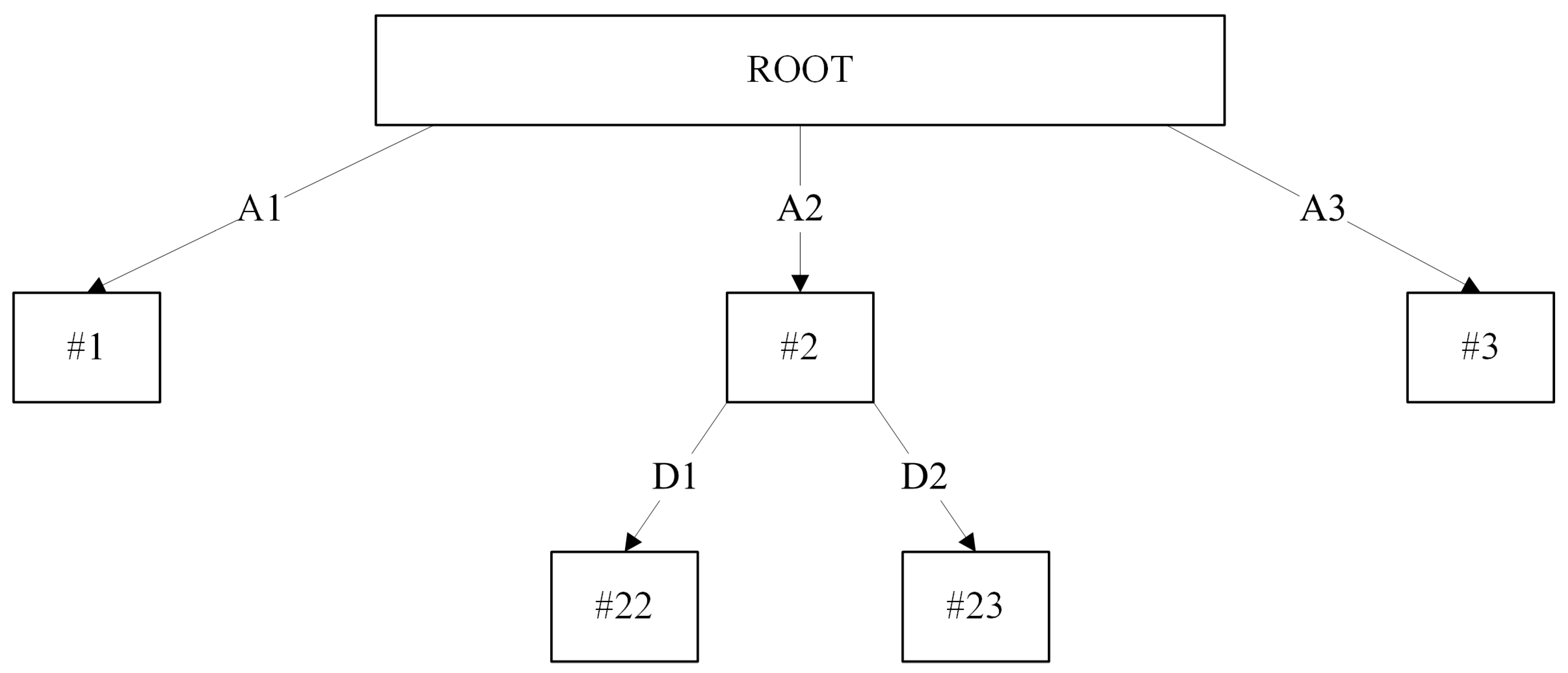
Assuming attribute value D2 is denoted as the confidential value, succeeding the sensitive pruning in Section 3.1 would result in the tree illustrated in Figure 3 and Figure 4. If the decision tree only splits based on two values, it is basically absurd to follow the sensitive pruning because a single split in the decision tree does not provide any significant benefit to the current tree. Therefore, we proposed to prune all of the descendants (subtree) of node #2 when the number of splits is equivalent to two, converting node #2 into a leaf node.
The optimistic sensitive pruning algorithm can be summarized as follows in Algorithm 2:
Algorithm 2: Optimistic Sensitive Pruning Algorithm
Input:
    Tmax, Unpruned Decision Tree
    Sensitive Attribute Value, AS
Output:
    Pruned Sensitive Decision Tree
Procedure:
Learning Procedure I:
1.  for all split in node t, do
2.  Let node ts be the child node of t
3.  Let Attribute Value A equals to current split attribute value
4.  if (A == AS):
5.      Replace A value with “SENSITIVE”
6.      if (ts contains any child node):
7.           Replace ts with a leave node
8.      endif
9.      if (number of split == 2):
10.       Replace t with a leave node
11.    endif
12.   endif
13. endfor
Learning Procedure II:
14. Let T = Tmax
15. if T is not “leave node”:
16.     for all node tT, starting from leaf nodes towards the root node, do
17.          Repeat step 1–13
18.     endfor
19. endif

3.3. Pessimistic Sensitive Pruning

In the scenario whereby privacy is given the highest priority, we would remove the entire same-level subtree when the sensitive value is detected. For example, Figure 2, consisting of the confidential attribute value B3, will result in Figure 5 by using the pessimistic sensitive pruning. The essential benefit from this pruning approach is the privacy is preserved, as the attribute does not even exist in the decision tree. The primary inspiration of this pruning approach is the ideology of guessing theory, assuming that attribute values B1 and B2 are equal to ‘low’ and ‘medium’. One can easily predict the value of B3 to be equivalent to ‘high’. Therefore, each of the suggested pruning algorithms is able to provide different privacy requirements depending on the user’s preference.
Pessimistic sensitive pruning algorithm is summarized as follows in Algorithm 3:
Algorithm 3: Pessimistic Sensitive Pruning Algorithm
Input:
    Tmax, Unpruned Decision Tree
    Sensitive Attribute Value, AS
Output:
    Pruned Sensitive Decision Tree
Procedure:
Learning Procedure I:
1.  for all split in node t, do
2.      Let node ts be the child node of t
3.      Let Attribute Value A equals to current split attribute value
4.      if (A == AS):
5.       Replace t with a leave node
6.      endif
7.  endfor
Learning Procedure II:
8.  Let T = Tmax
9.  if T is not “leave node”:
10.   for all node tT, starting from leaf nodes towards the root node, do
11.        Repeat step 1–7
12.   endfor
13. endif

3.4. Sensitive Values Considerations

Sensitive attributes and values can vary significantly across different domains; therefore, domain knowledge or the input of domain experts is typically required to determine which attributes should be considered sensitive. In this work, sensitive attributes and values were identified based on established knowledge in the field of NIDSs (for example, private IP addresses and host-specific identifiers). Although no domain experts were directly consulted, these attributes reflect widely accepted sensitivity indicators reported in prior NIDS research. The same principle can be extended to other domains, such as finance or healthcare, by tailoring the sensitivity list to domain-specific requirements (for example, account numbers or patient identifiers).

3.5. Privacy Risk Metrics Considerations

The primary goal of the sensitive pruning algorithm is to minimize the exposure of sensitive attribute values within the decision tree nodes. However, the publicly available NIDS datasets used in this study do not provide ground-truth annotations indicating which attributes are sensitive. Consequently, widely adopted privacy risk metrics such as k-anonymity or differential privacy could not be applied. Instead, we approximate privacy preservation by evaluating structural simplification of the decision tree, specifically through the number of sensitive nodes removed and the overall reduction in tree complexity. This approach aligns with the objective of concealing sensitive splits while maintaining classification utility.

3.6. GDPR-Compliant Model Sharing

The General Data Protection Regulation (GDPR) emphasizes data minimization and pseudonymization to support safer sharing of machine learning models in critical domains such as healthcare, finance, and network security. The proposed sensitive pruning strategies align with these principles by concealing sensitive attribute values within decision tree models. Through the replacement or removal of sensitive nodes, the resulting pruned trees reduce the risk of exposing personally identifiable information, such as private IP addresses. While our experiments focus on publicly available NIDS datasets, these strategies can be readily applied to other privacy-critical domains to facilitate GDPR-compliant model sharing during collaborative research and deployment.

4. Application and Motivation

To demonstrate the capability of our proposed pruning algorithm, we adopted the post-pruning method in the domain of NIDS. Traditionally, NIDS relies on the signature database in Snort for detecting malicious traffic. With the explosion of machine learning, many techniques involving the use of artificial intelligence have been widely proposed by researchers for detecting malicious packets [60,61,62]. It is necessary to supply huge and quality-labeled training data for building a machine classifier with high performance. In NIDS, the training data generally refers to the network traces information extracted from the packets. Some of the common information found in packets includes IP addresses, port numbers, TCP flags, transport protocol, etc.
While both the independent field of privacy-preserving decision trees [6,63,64] and privacy solutions [65,66] in the domain of NIDS have been explored for quite some time, none of the literature has yet to study the combination of them. At a glance, a decision tree model built upon sets of network traces data might appear to be non-intrusive. To illustrate the concepts of privacy leakage for decision trees in NIDS, Figure 6 is generated for portraying the described scenario.
Referring to Figure 6, several pieces of inductive information can be inferred. For instance, there is a high possibility of opened TCP port 22 for the IP address of 192.168.32.7. Further analysis by a domain expert might reveal that secure shell services are made available for the host with the unique IP address of 192.168.32.7 [67]. Zhang et al. [68] and Coull et al. [69] state that services operating on a specific host can be uncovered by utilizing mappings of port numbers to services. Subsequently, adversaries can then launch an attack on an individual or organization by exploiting the information discovered [70]. Although researchers have proposed various approaches for concealing the IP addresses [66,71,72,73] while retaining their unique characteristics for network analysis purposes along with a decent level of privacy protection, some of the methods suffer from re-identification attacks [74]. Moreover, it is also not an easy task to maintain the consistency of IP address anonymization (pseudonymization) across various network trace datasets over a period of time. On top of that, the utility of the anonymization solution is questionable when tested against the traditional Snort IDS [65,66]. Hence, we proposed to take a different approach in safeguarding the privacy by adopting the proposed pruning algorithms described in Section 3.
Before conducting the experiments, it is important to first define the confidential attribute values as required by our pruning algorithms. Due to the lack of domain experts, we proposed the confidential values to encompass all private IP addresses because the range can resemble a group of IP addresses for an organization. The full list of private IP addresses is tabulated in Table 1.

5. Experiment

5.1. Datasets and Experimental Settings

To evaluate the effect of our proposed pruning algorithms, several experiments have been conducted against 3 publicly available NIDS datasets: GureKDDCup [75,76], UNSW-NB15 [77], and CIDDS-001 [78]. The three mentioned datasets are utilized in our work because they contain the missing pair of IP attributes from the benchmark NIDS datasets (KDDCup 99′ [79] and NSL-KDD [80]). It is not plausible for us to perform any experiments utilizing the proposed privacy pruning without the pairs of IP addresses. Several recent reviews of the NIDS datasets are published in [62,81,82]. Datasets adopted in our studies are summarized and tabulated in Table 2.
To fairly judge the performance of each machine learner, no (minimal) data cleansing and pre-processing are performed against the datasets employed for conforming the classifiers data requirements. Each of the description and pre-processing steps for the datasets are thoroughly explained in Section 5.1.1, Section 5.1.2 and Section 5.1.3. Since the standard tenfold cross validation [83] is not suitable to be adopted due to temporal dependencies and data leakage risks, we utilized a rolling-origin resampling scheme for training and testing distribution, following the methodology presented in our previous benchmarking study [84]. Rolling-origin, widely used in time-series forecasting, progressively expands the training set while moving the testing window forward, providing a more realistic and unbiased evaluation for NIDS datasets. The detailed train-test splits using this approach are illustrated in the subsequent subsection.

5.1.1. GureKDDCup Dataset and Pre-Processing

GureKDDCup [75,76] was released in 2008 to complement the drawback of the KDDCup 99′ [80] NIDS datasets. As KDDCup 99′ is more than several decades old, researchers have deemed the datasets to be obsolete in reflecting the present network traffics [85,86]. GureKDDCup was generated by imitating the similar procedure of creating the KDDCup 99′. Additionally, payloads, IP addresses, and port numbers, which are missing from the KDDCup 99′, are incorporated into the dataset. On top of that, the creators of GureKDDCup have also included several new attacks that are absent in KDDCup 99′. The full version of the GureKDDCup dataset is compressed into a 9.3 GB file (gureKddcup.tar.gz). The file size is tremendously huge due to the added payloads data to each of the network traffics. However, we only used the daily logs found in each gureKddcup-matched.list for the experiment conducted. Each of the daily logs are concatenated and merged into a single file containing a week of network traffic. Table 3 shows the total number of instances available in each week, while Table 4 presents the distribution of training and testing data in accordance with the number of weeks. No data cleansing, feature extraction, or attribute reduction is necessary to be performed against the GureKDDCup dataset.

5.1.2. UNSW-NB15 Dataset and Pre-Processing

Moustafa et al. [77] released the UNSW-NB15 dataset in 2015 to complement the lack of footprint attacks [81] in KDDCup 99′ [79]. Although the documentation stated a total number of instances equivalent to 2,540,044, we have verified that an additional instance is found in each week (weeks 1, 2, and 3), leading to a total of 2,540,047 instances. As shown in Table 5, some data cleansing is unavoidable; it is necessary to be conducted against the dataset before we are able to build the machine learner. The label attribute, which consists of a binary class {normal, attack}, was discarded as we employ the attack_cat containing 10 different classes as our class label. Table 6 tabulated the number of instances contained in each week, while Table 7 provides the partition of training and testing data distribution. It is also worth mentioning that although UNSW-NB15 has provided a small version of the dataset, the absence of IP addresses in the small version prohibits us from performing our experiment against it.

5.1.3. CIDDS-001 Dataset and Pre-Processing

The CIDDS-001 NIDS [78] dataset has been publicly available since 2017. The dataset contains a total of 32 million flows, whereby 31 million are from the emulated internal environment (Openstack software); and 0.7 million are from the external traffic consisting of real traffic from the internet. We have excluded the external traffic from our experiment due to inaccurate labels and the absence of some attacks. The full CIDDS-001 Openstack internal traffic is employed in the experimental procedure. Table 8 shows some of the data cleansing necessary to be performed against the dataset. The entire flows attribute was removed from the dataset, as it contains only a single constant value for all instances [81]. In the case of flags, we have split the single-attribute flags into five distinct flags in accordance with their value. The IP addresses are modified in such a way that they will not collide with other IP addresses and match the dot separator of IP addresses. The total number of instances for each week are tabulated in Table 9. while the training and testing data distribution is presented as shown in Table 10. A significant reason for excluding the week 3 and 4 data from the experimental procedure is because it only encompassed normal traffic.

5.2. Types of Pruning, Evaluation Metrics, and Experimental Setup

As discussed in Section 3.1, three variants of sensitive pruning are proposed in this paper. To compare the performance of the designed algorithm, the experimental results of J48 with and without the default pruning are compared empirically. Additionally, three hybrid pruning algorithms incorporating the default J48 pruning and the proposed sensitive pruning algorithms are also implemented. It should be noted that our program will perform the default J48 pruning algorithm ahead of the proposed sensitive pruning. Table 11 summarizes all of the pruning procedures employed in this paper.
Three performance evaluation metrics are used in comparing the empirical results, including (i) classification accuracy, (ii) number of pruned nodes, and (iii) number of final nodes. The number of pruned nodes is calculated by accumulating the number of nodes pruned by the sensitive pruning (inclusive of the sensitive nodes as depicted in Figure 2 in Section 3.1) as well as the J48 pruning. For the number of final nodes, the final model of the decision tree nodes will exclude the nodes splitting with the value of “SENSITIVE”. This is because the nodes are no longer significant in the classification process.
All of the aforementioned pruning algorithms in Table 11 are performed on the same computing environment with the hardware specification of an eight-core 3.64 GHz AMD Ryzen CPU and 64 GB RAM on Windows 10. The Weka J48 package (stable version 3.8) is employed for extending the default pruning algorithm throughout the entire experiment.

5.3. Experimental Results

5.3.1. Performance Comparison of All Pruning Algorithms

Experimental results based on the pruning described in Section 5.2 are tabulated in Table 12 and Table 13. All of the performed experiments follow the aforementioned dataset distribution as explained in Section 5.1. From both Table 12 and Table 13, the performance of the proposed pruning algorithm is very encouraging, as most of the proposed model only suffers a slight loss in terms of accuracy as compared to the unpruned tree (J48U-NO). Although the classification accuracy has slightly decreased, the number of nodes removed by the sensitive pruning escalates substantially. Additionally, the hybrid version of pruning, consisting of the default J48 pruning and sensitive pruning, further reduced the number of nodes available in the final model. In the case of a decision tree, a smaller tree with a satisfactory classification accuracy is much preferred over a highly complex tree that overfits the training data. This is because a smaller tree improves the readability and interpretability of a decision tree.
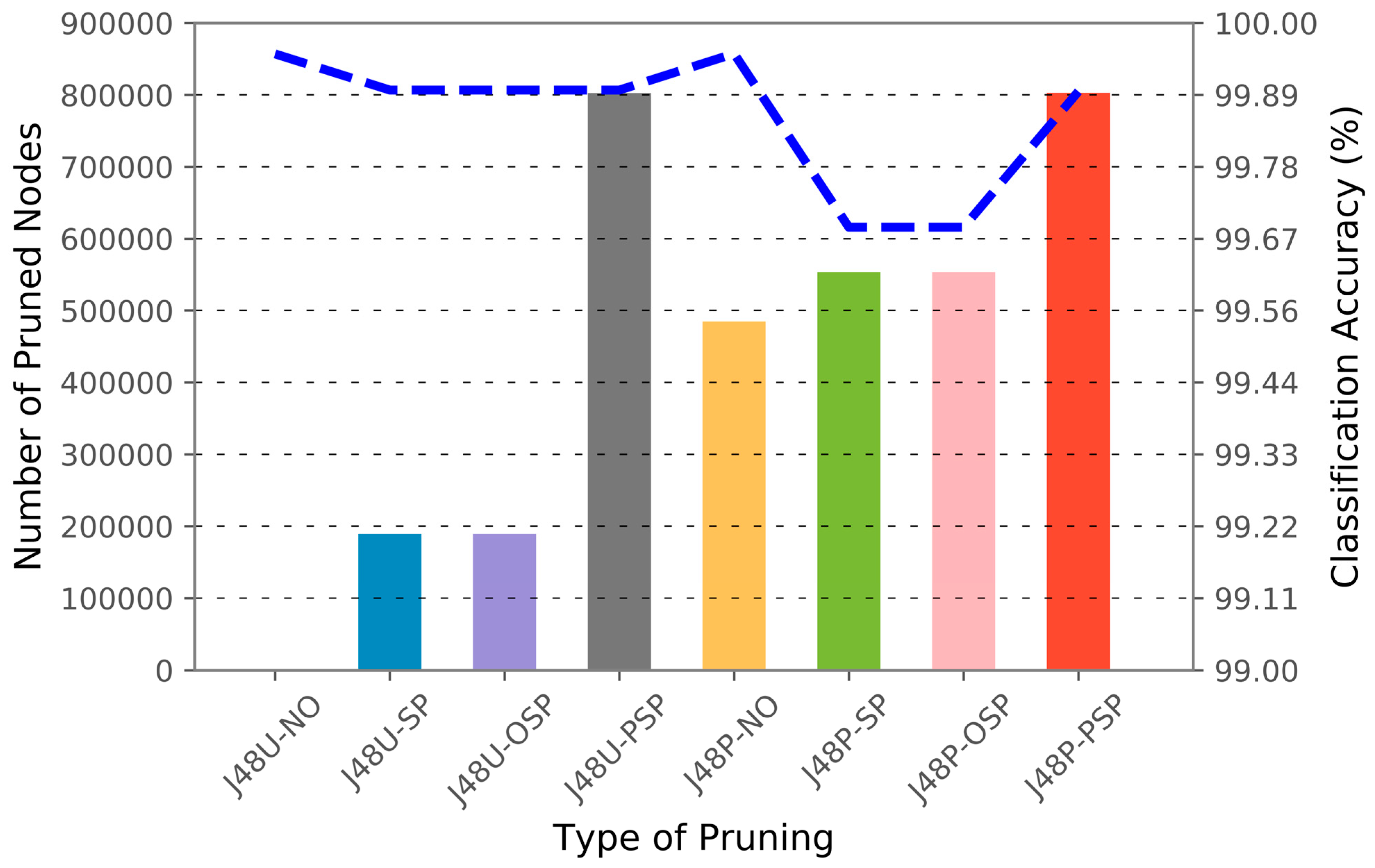
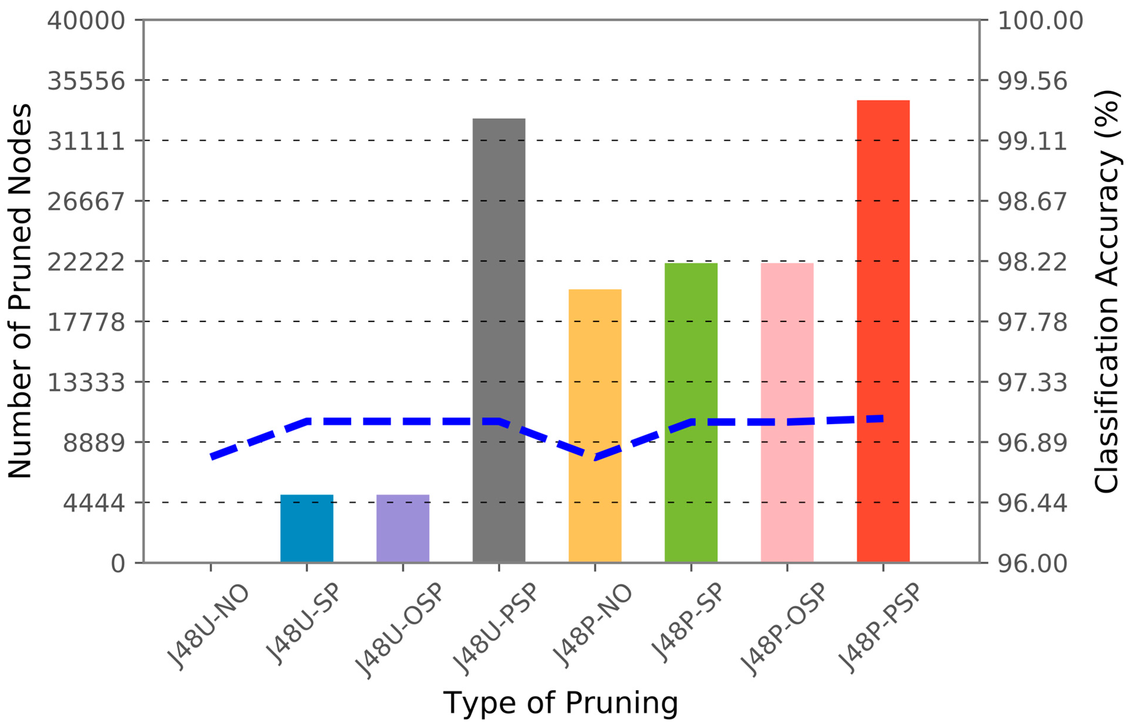
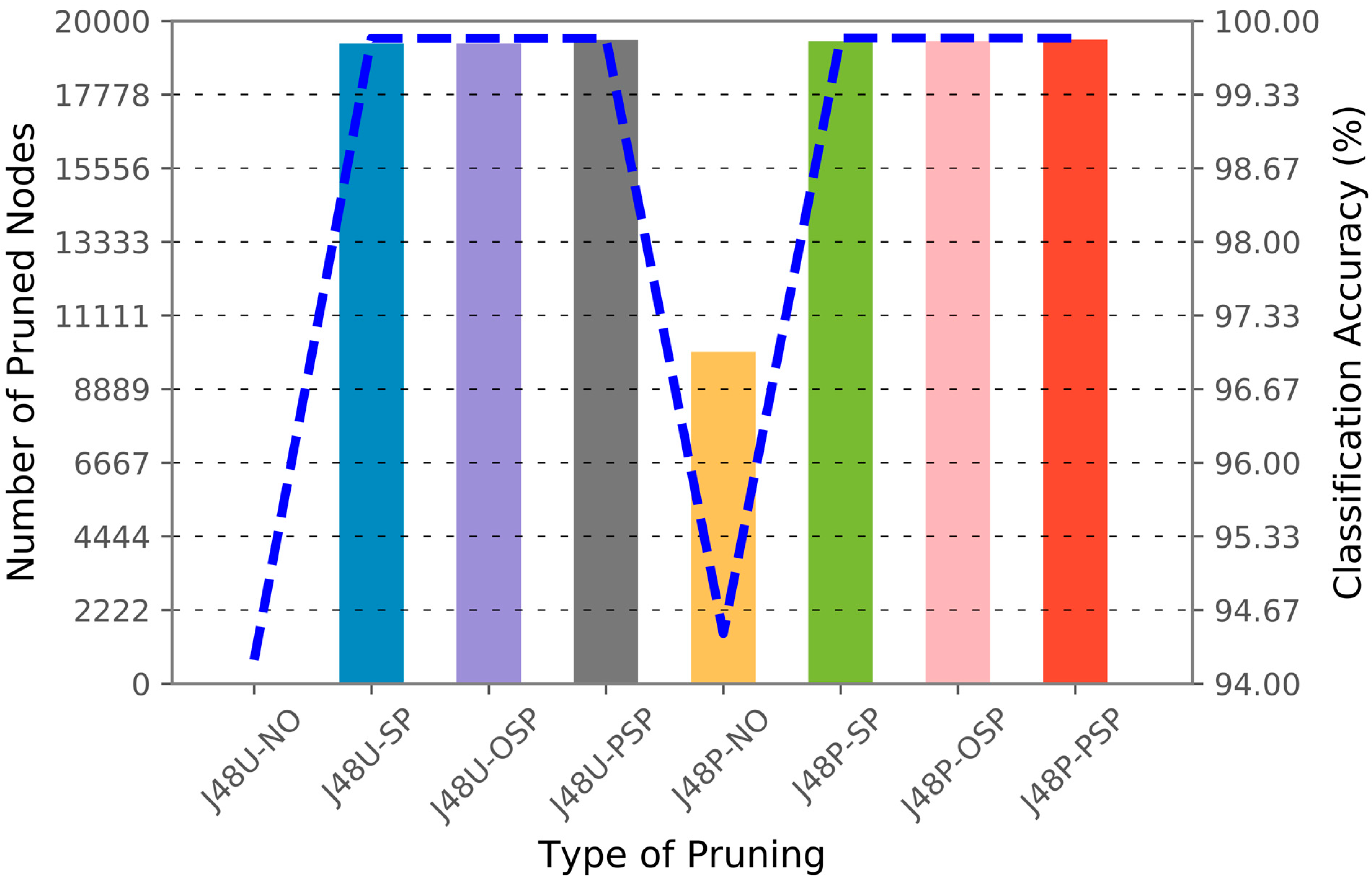
To illustrate the relationship between the pruning algorithm, classification accuracy, and the number of pruned nodes, Figure 7, Figure 8 and Figure 9 are generated in accordance with each dataset. The number of pruned nodes can be clearly seen to escalate when J48 default pruning is applied with sensitive pruning for the GureKDDCup (Figure 7) and UNSW-SB15 (Figure 8) datasets. However, we observed a constant number of pruned nodes and classification accuracy when either one of the sensitive pruning methods was applied against the CIDDS-001 dataset. This can be explained by the ratio of the number of unique IP addresses against the number of unique private IP addresses in the dataset. As shown in Table 14, 34 out of 38 source IP addresses and 785 out of 790 destination IP addresses in CIDDS-001 are comprised of private IP addresses. Referring to the three figures, we observe that the number of pruned nodes and classification accuracy remain constant for both J48U-SP and J48U-OSP. After analyzing the decision rules in the model, the scenario can be justified, as all of the IP addresses in the decision tree always split into more than 2 branches. Thus, leading the J48U-OSP to have the same effects as J48U-SP. The hybrid pruning J48P-SP and J48P-OSP are observed to be having the similar effects as they are built upon the identical sensitive pruning (J48U-SP, J48U-OSP). From the empirical results attained in this section, we proved that the privacy of attribute values can be preserved in a decision tree in exchange for a small loss of classification accuracy.

5.3.2. Visibility of Sensitive Information in Decision Tree

Sensitive pruning, optimistic sensitive pruning, and pessimistic sensitive pruning are sensitive pruning extensions established upon the default J48 Weka decision tree package. Adopting the similar properties from a decision tree, the tree-like structure of a model remains. Thus, the classification information and splitting values, except the predefined sensitive values, in the final model of the proposed pruning are made visible. The availability of this information will allow the domain expert (e.g., system administrator) to interpret and have a better understanding regarding the current situation of the network. For the sake of simplicity, a partial of the ASCII J48U-SP tree model built against the CIDDS-001 dataset is shown in Figure 10. The results obtained are based on the train-test data distribution as tabulated in Table 10.
As mentioned earlier in Section 3.1, retaining or removing the sensitive nodes would not directly affect the classification performance of the decision tree model. Therefore, several options are provided to the users for flexibility in displaying the classification information on the sensitive nodes. Depending on the requirement, the resulting decision tree model can (i) show the label (class) and distribution of the sensitive nodes as shown in Figure 10, (ii) show only an attribute value containing “SENSITIVE”, or (iii) directly remove the entire sensitive nodes from the model.

5.3.3. Computational Complexity Comparison Against All Pruning Algorithms

As described in Section 5.3.1, the advantages of a small tree over a complex tree include the simplicity in interpreting and understanding the decision rules. On top of that, a smaller tree with fewer nodes would probably require less time for the model to evaluate the test instances. This is because when the test instances traverse from the root node to the decision (leaf) node, a lesser node would be necessary for the test instances to move in a smaller tree.
To substantiate our hypothesis, the computation time for evaluating the test instances with each of the proposed pruning algorithms is tabulated in Table 15. Referring to Table 15, most of the proposed sensitive pruning algorithms required less time as compared to the tree without pruning (J48U-NO). The most noticeable dataset that benefitted from the smaller size of the tree is CIDDS-001. Although the proposed pruning algorithms are able to decrease the model evaluation time, most of them require a little extra time in building the proposed model. As shown in Table 16, almost all of the proposed pruning algorithms consume more time in contrast to the unpruned model (J48U-NO) and standard J48 pruned model (J48P-NO). This scenario is entirely justifiable, as all of the pruning algorithms are mandatory in building the full decision tree model before removing any insignificant nodes. Although there is a slight increase in time required for building the decision tree model, the additional time is still acceptable because the privacy of information is able to be preserved in exchange for some computational resources.
While sensitive pruning effectively reduces tree size and slightly decreases evaluation time, it introduces additional computational steps during tree construction. Each sensitive attribute check requires a full traversal of the decision tree, resulting in computational overhead proportional to both the number of sensitive attributes and the number of nodes (approximately O k · n , where k is the number of sensitive attributes and n is the node count). In our experiments, this overhead is negligible even for the largest dataset (CIDDS-001, with approximately 18 million records) due to the pruning being performed offline during model training. In real-time intrusion detection, inference speed is critical, and the reduced tree size from pruning directly benefits detection latency.

5.3.4. Application of Anonymization Algorithm: Truncation and Bilateral Classification

In principle, anonymization solution would definitely destroy or degrade the original dataset to a certain extent. From the experimental results obtained by Mivule et al. [87,88], the Iris dataset that is applied with data privacy solutions (noise) always results in higher classification errors when compared against the original dataset. However, the scenarios observed are not always true based on the empirical results acquired in our previous work.
Motivated by our previous studies [89,90] related to the various anonymization techniques on network traces data, we have proven that some of the anonymization techniques are suitable to be adopted for improving the performance of classifiers. For instance, our first studies [89] convince us of the suitability and possibility of an anonymization solution (e.g., bilateral classification performed against port numbers) for raising the classification accuracy of the J48 decision tree model. Inspired by our first studies, we subsequently performed IP address truncation [90] with 10 different machine learning classifiers against the 6 percent GureKDDCup [75] NIDS dataset. The empirical results obtained are very encouraging because the classification accuracy for 4 out of the 10 classifiers has actually improved, and the time taken for building the model for 7 out of the 10 classifiers is reduced significantly. Additionally, the results attained also verified the capability of the IP anonymization solution (IP address truncation) as a dimensionality reduction technique in the domain of machine learning.
With the strength and advantages of the data privacy algorithms discussed in our previous works, we have applied the similar anonymization solutions with our proposed pruning algorithms against all of the NIDS datasets in this paper to safeguard a higher level of privacy. For simplicity, the experimental results shown only include the combination of bilateral classification on both source and destination port numbers as well as 24-bit (3-octet) IP address truncation against both source and destination IP addresses. To provide a fair comparison between the experiments conducted in Section 5.3.1, similar datasets and experimental procedures are employed. The empirical results adopting both the anonymization solution and all of the proposed pruning algorithms are tabulated in Table 17 and Table 18. The total number of unique IP addresses after applying the 24-bit IP address truncation is also shown in Table 14.
To scrutinize the difference in performance, Table 19 is generated by measuring the mathematical difference in empirical results in Section 5.3.1 and Section 5.3.4. Referring to Table 19, interesting results are observed when J48U-NO is applied against the GureKDDCup week 1 and 1~2 training data, whereby the accuracy is increased by 47.61% and 51.45% when the privacy solution is applied. As shown in Table 19, we noticed that the number of final nodes is significantly reduced for most of our proposed algorithms in all datasets. At the same time, our proposed algorithm suffers a small loss (approximately less than ~1%) in classification accuracy when tested against all the datasets. The trade-off is obviously worth it because we are able to secure a higher level of privacy in a smaller tree by sacrificing a small loss of accuracy. As mentioned earlier, a smaller tree would undoubtedly benefit the users in interpreting a decision tree model. The experimental results obtained further substantiate our claims that not all data privacy algorithms would degrade the quality of data; some of the anonymization solutions are suitable to be utilized as a grouping mechanism or dimensionality reduction in the domain of machine learning for improving the performance of a classifier.

5.3.5. Benchmarking Against Other Machine Learning Models

To compare the performance of the proposed sensitive pruning algorithms, we conducted benchmark testing against ten widely used machine learning classifiers available in the Weka package: ZeroR, Random Tree, REPtree, Decision Stump, AdaBoost, BayesNet, Naïve Bayes, Random Forest, and Support Vector Machine (SMO). Due to limited prior experiments on the adopted datasets, results for these classifiers were taken from our previous work [84]. For comparability, only the results corresponding to the largest training–testing splits are considered: GureKDDCup (Train: 1–6; Test: 7), UNSW-NB15 (Train: 1–3; Test: 4), and CIDDS-001 (Train: 1; Test: 2). Results for the proposed pruning algorithms are taken from Table 12 and Table 13.
Table 20 presents the classification accuracies for all baseline models and pruning strategies across the three datasets, while Figure 11 illustrates the comparative results. As shown in Figure 11, the proposed sensitive pruning algorithms (J48U-SP, J48U-OSP, J48U-PSP, and their hybrid counterparts) achieved classification accuracies comparable to, and in some cases exceeding, those of strong baselines such as Random Forest. Notably, the pruned models consistently maintained high performance while simultaneously reducing tree complexity and concealing sensitive attributes, thereby offering both interpretability and privacy advantages. This demonstrates that privacy-preserving decision tree pruning can achieve competitive utility while fulfilling stricter privacy requirements in critical domains.

6. Conclusions

In this paper, pruning approaches with privacy considerations are proposed, namely Sensitive Pruning (SP), Optimistic Sensitive Pruning (OSP) and Pessimistic Sensitive Pruning (PSP). All three of the proposed algorithms are enhanced based on the Weka J48 (C4.8) model. The designed solutions removed (“pruned”) nodes containing sensitive information from the final decision tree model. Additionally, we also integrated the proposed algorithms with the default J48 pruning algorithm. Based on the promising evaluation results tested against the three publicly available NIDS datasets, the proposed privacy pruning spells the following four advantages: (1) preserving privacy by discarding sensitive IP addresses from the tree model with a small sacrificial loss in terms of accuracy; (2) visibility of classification rules except rules containing sensitive information; (3) a smaller tree with fewer nodes that leads to lower computational time necessary for evaluating the test instances; and (4) suitability of the network traces privacy solution algorithm (port number bilateral classification and IP address truncation) in safeguarding the sensitive information and improving the performance of a model.
For future works, we plan to extend our work so that (1) it is flexible enough to be applied across various domains, (2) it resolves the instability when sensitive values are detected at the higher level of the decision tree, (3) it incorporates formal privacy risk metrics such as k-anonymity or differential privacy to measure privacy leakage and (4) it explores optimizations, including incremental pruning, streaming-based updates, and GPU or multi-core parallelism, to ensure scalability in high-throughput or real-time environments.

Author Contributions

Conceptualization, Y.J.C.; methodology, Y.J.C. and S.Y.O.; formal analysis, Y.J.C. and S.Y.O.; investigation, Y.J.C.; visualization, Y.J.C. and Z.Y.L.; writing—original draft, Y.J.C.; funding acquisition, S.Y.O.; resources, S.Y.O.; project administration, S.Y.O.; supervision, S.Y.O. and Y.H.P.; writing—review and editing, S.Y.O., Y.H.P. and Z.Y.L. All authors have read and agreed to the published version of the manuscript.

Funding

This research work was supported by a Fundamental Research Grant Scheme (FRGS) under the Ministry of Education and Multimedia University, Malaysia (Project ID: MMUE/160029).

Data Availability Statement

The original datasets presented in the study are openly available in [76] GureKDDCup at https://aldapa.eus/res/gureKddcup/ (accessed on 3 August 2025), [77] UNSW-NB15 at https://research.unsw.edu.au/projects/unsw-nb15-dataset, (accessed on 3 August 2025), and [78] CIDDS-001 at https://www.hs-coburg.de/forschen/cidds-coburg-intrusion-detection-data-sets/. (accessed on 3 August 2025).

Conflicts of Interest

The authors declare no conflicts of interest.

Abbreviations

The following abbreviations are used in this manuscript:
AAAdaptive Apriori
AAAoP-DTAdaptive Apriori post-pruned Decision Tree
CARTsClassification and Regression Trees
CCPCost–Complexity Pruning
CSPCost-Sensitive Pruning
CVPCritical Value Pruning
DIDepth–Impurity
EBPerror-based pruning
IEEPImproved Expected Error Pruning
IQNImpurity Quality Node
KLKullback–Leibler
MEPMinimum Error Pruning
NIDSNetwork Intrusion Detection System
OPTOptimal Pruning Algorithm
PEPPessimistic Error Pruning
PSOParticle Swarm Optimization
REPReduced Error Pruning
ROCReceiver Operating Characteristics
BMRBayes Minimum Risk

References

  1. Fung, B.C.M.; Wang, K.; Chen, R.; Yu, P.S. Privacy-Preserving Data Publishing. ACM Comput. Surv. 2010, 42, 1–53. [Google Scholar] [CrossRef]
  2. Nettleton, D. Chapter 18: Data Privacy and Privacy-Preserving Data Publishing. In Commercial Data Mining: Processing, Analysis and Modeling for Predictive Analytics Projects; Morgan Kaufmann Publishers Inc.: San Francisco, CA, USA, 2014; pp. 217–228. ISBN 0124166024/9780124166028. [Google Scholar]
  3. Aggarwal, C.C.; Yu, P.S.-L. A General Survey of Privacy-Preserving Data Mining Models and Algorithms. In Privacy-Preserving Data Mining: Models and Algorithms; Springer: Boston, MA, USA, 2008; Volume 34, pp. 11–52. [Google Scholar] [CrossRef]
  4. Aldeen, Y.A.A.S.; Salleh, M.; Razzaque, M.A. A Comprehensive Review on Privacy Preserving Data Mining. Springerplus 2015, 4, 694. [Google Scholar] [CrossRef] [PubMed]
  5. Dhivakar, K.; Mohana, S. A Survey on Privacy Preservation Recent Approaches and Techniques. Int. J. Innov. Res. Comput. Commun. Eng. 2014, 2, 6559–6566. [Google Scholar]
  6. Li, X.-B.; Sarkar, S. Against Classification Attacks: A Decision Tree Pruning Approach to Privacy Protection in Data Mining. Oper. Res. 2009, 57, 1496–1509. [Google Scholar] [CrossRef]
  7. Quinlan, J.R. Induction of Decision Trees. Mach. Learn. 1986, 1, 81–106. [Google Scholar] [CrossRef]
  8. Quinlan, J.R. C4.5: Program for Machine Learning; Morgan Kaufmann Publishers Inc.: San Mateo, CA, USA, 1993; ISBN 1-55860-238-0. [Google Scholar]
  9. Breiman, L.; Friedman, J.; Stone, C.J.; Olshen, R.A. Classification and Regression Trees; Taylor & Francis: Oxfordshire, UK, 1984. [Google Scholar]
  10. Chew, Y.J.; Ooi, S.Y.; Wong, K.-S.; Pang, Y.H. Decision Tree with Sensitive Pruning in Network-Based Intrusion Detection System BT—Computational Science and Technology; Alfred, R., Lim, Y., Haviluddin, H., On, C.K., Eds.; Springer: Singapore, 2020; pp. 1–10. [Google Scholar]
  11. Martin, J.K. An Exact Probability Metric for Decision Tree Splitting and Stopping. Mach. Learn. 1997, 28, 257–291. [Google Scholar] [CrossRef]
  12. Breslow, L.A.; Aha, D.W. Simplifying Decision Trees: A Survey. Knowl. Eng. Rev. 1997, 12, 1–40. [Google Scholar] [CrossRef]
  13. Frank, E.; Witten, I.H. Reduced-Error Pruning with Significance Tests; Department of Computer Science, University of Waikato: Hamilton, New Zealand, 1999. [Google Scholar]
  14. Quinlan, J.R. Simplifying Decision Trees. Int. J. Man. Mach. Stud. 1987, 27, 221–234. [Google Scholar] [CrossRef]
  15. Mingers, J. An Empirical Comparison of Selection Measures for Decision Tree Induction. Mach. Learn. 1989, 3, 319–342. [Google Scholar] [CrossRef]
  16. Esposito, F.; Malerba, D.; Semeraro, G.; Kay, J. A Comparative Analysis of Methods for Pruning Decision Trees. IEEE Trans. Pattern Anal. Mach. Intell. 1997, 19, 476–491. [Google Scholar] [CrossRef]
  17. Costa, V.G.; Pedreira, C.E. Recent Advances in Decision Trees: An Updated Survey. Artif. Intell. Rev. 2023, 56, 4765–4800. [Google Scholar] [CrossRef]
  18. Harviainen, J.; Sommer, F.; Sorge, M.; Szeider, S. Optimal Decision Tree Pruning Revisited: Algorithms and Complexity. arXiv 2025, arXiv:2503.03576. [Google Scholar]
  19. Esposito, F.; Malerba, D.; Semeraro, G. Simplifying decision trees by pruning and grafting: New results (Extended abstract). In Machine Learning: ECML-95. ECML 1995, Lecture Notes in Computer Science; Lavrac, N., Wrobel, S., Eds.; Springer: Berlin/Heidelberg, Germany, 1995; Volume 912. [Google Scholar] [CrossRef]
  20. Witten, I.H.; Frank, E.; Hall, M.A.; Christopher, J.P. Data Mining: Practical Machine Learning Tools and Techniques, 3rd ed.; Elsevier: Amsterdam, The Netherlands, 2011; ISBN 9780128042915. [Google Scholar] [CrossRef]
  21. Jensen, D.; Schmill, M.D. Adjusting for Multiple Comparisons in Decision Tree Pruning. In Proceedings of the 3rd International Conference on Knowledge Discovery and Data Mining, Newport Beach, CA, USA, 14–17 August 1997; pp. 195–198. [Google Scholar] [CrossRef]
  22. Cestnik, B.; Bratko, I. On Estimating Probabilities in Tree Pruning. In Lecture Notes in Computer Science; Springer: Berlin/Heidelberg, Germany, 1991; Volume 482, pp. 138–150. [Google Scholar] [CrossRef]
  23. Watkins, C.J.C.H. Combining Cross-Validation and Search. In Proceedings of the 2nd European Conference on European Working Session on Learning, Bled, Yugoslavia, 1 May 1987; Sigma Press: Rawalpindi, Pakistan, 1987; pp. 79–87. [Google Scholar]
  24. Zhang, Y.; Chi, Z.X.; Wang, D.G. Decision Tree’s Pruning Algorithm Based on Deficient Data Sets. In Proceedings of the Sixth International Conference on Parallel and Distributed Computing Applications and Technologies (PDCAT’05), Dalian, China, 5–8 December 2005; Volume 2025, pp. 1030–1032. [Google Scholar] [CrossRef]
  25. Mitu, M.M.; Arefin, S.; Saurav, Z.; Hasan, M.A.; Farid, D.M. Pruning-Based Ensemble Tree for Multi-Class Classification. In Proceedings of the 2024 6th International Conference on Electrical Engineering and Information & Communication Technology (ICEEICT), Mirpur, Dhaka, 2–4 May 2024; IEEE: Dhaka, Bangladesh, 2024; pp. 481–486. [Google Scholar]
  26. Gelfand, S.B.; Ravishankar, C.S.; Delp, E.J. An Iterative Growing and Pruning Algorithm for Classification Tree Design. IEEE Trans. Pattern Anal. Mach. Intell. 1991, 13, 163–174. [Google Scholar] [CrossRef]
  27. Bohanec, M.; Bratko, I. Trading Accuracy for Simplicity in Decision Trees. Mach. Learn. 1994, 15, 223–250. [Google Scholar] [CrossRef]
  28. Almuallim, H. An Efficient Algorithm for Optimal Pruning of Decision Trees. Artif. Intell. 1996, 83, 347–362. [Google Scholar] [CrossRef]
  29. Lazebnik, T.; Bunimovich-Mendrazitsky, S. Decision Tree Post-Pruning without Loss of Accuracy Using the SAT-PP Algorithm with an Empirical Evaluation on Clinical Data. Data Knowl. Eng. 2023, 145, 102173. [Google Scholar] [CrossRef]
  30. Bagriacik, M.; Otero, F. Fairness-Guided Pruning of Decision Trees. In Proceedings of the 2025 ACM Conference on Fairness, Accountability, and Transparency, Athens, Greece, 23–26 June 2025; Association for Computing Machinery: New York, NY, USA, 2025; pp. 1745–1756. [Google Scholar]
  31. Osei-Bryson, K.-M. Post-Pruning in Decision Tree Induction Using Multiple Performance Measures. Comput. Oper. Res. 2007, 34, 3331–3345. [Google Scholar] [CrossRef]
  32. Fournier, D.; Crémilleux, B. A Quality Index for Decision Tree Pruning. Knowl.-Based Syst. 2002, 15, 37–43. [Google Scholar] [CrossRef]
  33. Barrientos, F.; Sainz, G. Knowledge-Based Systems Interpretable Knowledge Extraction from Emergency Call Data Based on Fuzzy Unsupervised Decision Tree. Knowl.-Based Syst. 2012, 25, 77–87. [Google Scholar] [CrossRef]
  34. Wei, J.M.; Wang, S.Q.; You, J.P.; Wang, G.Y. RST in Decision Tree Pruning. In Proceedings of the Fourth International Conference on Fuzzy Systems and Knowledge Discovery (FSKD 2007), Haikou, China, 24–27 August 2007; Volume 3, pp. 213–217. [Google Scholar] [CrossRef]
  35. Pawlak, Z. Rough Sets. Int. J. Comput. Inf. Sci. 1982, 11, 341–356. [Google Scholar] [CrossRef]
  36. Wei, J.-M.; Wang, S.-Q.; Yu, G.; Gu, L.; Wang, G.-Y.; Yuan, X.-J. A Novel Method for Pruning Decision Trees. In Proceedings of the 2009 International Conference on Machine Learning and Cybernetics, Baoding, China, 12–15 July 2009; Volume 1, pp. 339–343. [Google Scholar]
  37. Osei-Bryson, K.-M. Post-Pruning in Regression Tree Induction: An Integrated Approach. Expert Syst. Appl. 2008, 34, 1481–1490. [Google Scholar] [CrossRef]
  38. Wang, H.; Chen, B. Intrusion Detection System Based on Multi-Strategy Pruning Algorithm of the Decision Tree. In Proceedings of the 2013 IEEE International Conference on Grey Systems and Intelligent Services (GSIS), Macao, China, 15–17 November 2013; pp. 445–447. [Google Scholar] [CrossRef]
  39. Knoll, U.; Nakhaeizadeh, G.; Tausend, B. Cost-Sensitive Pruning of Decision Trees. In Proceedings of the European Conference on Machine Learning, Catania, Italy, 6–8 April 1994; pp. 383–386. [Google Scholar]
  40. Bradley, A.; Lovell, B. Cost-Sensitive Decision Tree Pruning: Use of the ROC Curve. In Proceedings of the Eighth Australian Joint Conference on Artificial Intelligence, Canberra, Australia, 13–17 November 1995; pp. 1–8. [Google Scholar]
  41. Ting, K.M. Inducing Cost-Sensitive Trees via Instance Weighting. In Proceedings of the European Symposium on Principles of Data Mining and Knowledge Discovery, Nantes, France, 23–26 September 1998; pp. 139–147. [Google Scholar] [CrossRef]
  42. Bradford, J.P.; Kunz, C.; Kohavi, R.; Brunk, C.; Brodley, C.E. Pruning Decision Trees with Misclassification Costs. In Machine Learning ECML-98, Proceedings of the 10th European Conference on Machine Learning, Chemnitz, Germany, 21–23 April 1998; Springer: Berlin/Heidelberg, Germany, 1998; Volume 1398, pp. 131–136. [Google Scholar] [CrossRef]
  43. Chen, J.; Wang, X.; Zhai, J. Pruning Decision Tree Using Genetic Algorithms. In Proceedings of the 2009 International Conference on Artificial Intelligence and Computational Intelligence, Shanghai, China, 7–8 November 2009; Volume 3, pp. 244–248. [Google Scholar] [CrossRef]
  44. Zhang, W.; Li, Y. A Post-Pruning Decision Tree Algorithm Based on Bayesian. In Proceedings of the 2013 International Conference on Computational and Information Sciences, Shiyang, China, 21–23 June 2013; pp. 988–991. [Google Scholar] [CrossRef]
  45. Mehta, S.; Shukla, D. Optimization of C5.0 Classifier Using Bayesian Theory. In Proceedings of the 2015 International Conference on Computer, Communication and Control (IC4), Indore, India, 10–12 September 2015. [Google Scholar] [CrossRef]
  46. Malik, A.J.; Khan, F.A. A Hybrid Technique Using Binary Particle Swarm Optimization and Decision Tree Pruning for Network Intrusion Detection. Clust. Comput. 2017, 21, 667–680. [Google Scholar] [CrossRef]
  47. Sim, D.Y.Y.; Teh, C.S.; Ismail, A.I. Improved Boosted Decision Tree Algorithms by Adaptive Apriori and Post-Pruning for Predicting Obstructive Sleep Apnea. Adv. Sci. Lett. 2011, 4, 400–407. [Google Scholar] [CrossRef]
  48. Ahmed, A.M.; Rizaner, A.; Ulusoy, A.H. A Novel Decision Tree Classification Based on Post-Pruning with Bayes Minimum Risk. PLoS ONE 2018, 13, e0194168. [Google Scholar] [CrossRef]
  49. Bahnsen, A.C.; Stojanovic, A.; Aouada, D. Cost Sensitive Credit Card Fraud Detection Using Bayes Minimum Risk. In Proceedings of the 2013 12th International Conference on Machine Learning and Applications, Miami, FL, USA, 4–7 December 2013; Volume 1, pp. 333–338. [Google Scholar] [CrossRef]
  50. Frank, E.; Witten, I.H. Using a Permutation Test for Attribute Selection in Decision Trees. In Proceedings of the the 15th International Conference on Machine Learning, Madison, WI, USA, 24–27 July 1998; pp. 152–160. [Google Scholar]
  51. Crawford, S.L. Extensions to the CART Algorithm. Int. J. Man. Mach. Stud. 1989, 31, 197–217. [Google Scholar] [CrossRef]
  52. Efron, B.; Tibshirani, R. Improvements on Cross-Validation: The.632+ Bootstrap Method. J. Am. Stat. Assoc. 1997, 92, 548–560. [Google Scholar] [CrossRef]
  53. Scott, C. Tree Pruning with Subadditive Penalties. IEEE Trans. Signal Process. 2005, 53, 4518–4525. [Google Scholar] [CrossRef]
  54. García-Moratilla, S.; Martínez-Muñoz, G.; Suárez, A. Evaluation of Decision Tree Pruning with Subadditive Penalties. In Intelligent Data Engineering and Automated Learning—IDEAL 2006, Proceedings of International Conference on Intelligent Data Engineering and Automated Learning, Burgos, Spain, 20–23 September 2006; Sringer: Berlin/Heidelberg, Germany, 2006. [Google Scholar]
  55. Rissanen, J. Modeling by Shortest Data Description. Automatica 1978, 14, 465–471. [Google Scholar] [CrossRef]
  56. Mehta, M.; Rissanen, J.; Agrawal, R. MDL-Based Decision Tree Pruning. In Proceedings of the First International Conference on Knowledge Discovery and Data Mining, Montreal, QC, Canada, 20–21 August 1995; AAAI Press: Washington, DC, USA, 1995; pp. 216–221. [Google Scholar]
  57. Sweeney, L. K-ANONYMITY: A MODEL FOR PROTECTING PRIVACY. Int. J. Uncertain. Fuzziness Knowl.-Based Syst. 2002, 10, 557–570. [Google Scholar] [CrossRef]
  58. Pantoja, D.; Rodríguez, I.; Rubio, F.; Segura, C. Complexity Analysis and Practical Resolution of the Data Classification Problem with Private Characteristics. Complex. Intell. Syst. 2025, 11, 274. [Google Scholar] [CrossRef]
  59. Patil, D.D.; Wadhai, V.M.; Gokhale, J.A. Evaluation of Decision Tree Pruning Algorithms for Complexity and Classification Accuracy. Int. J. Comput. Appl. 2010, 11, 975–8887. [Google Scholar] [CrossRef]
  60. Tsai, C.F.; Hsu, Y.F.; Lin, C.Y.; Lin, W.Y. Intrusion Detection by Machine Learning: A Review. Expert. Syst. Appl. 2009, 36, 11994–12000. [Google Scholar] [CrossRef]
  61. Buczak, A.; Guven, E. A Survey of Data Mining and Machine Learning Methods for Cyber Security Intrusion Detection. IEEE Commun. Surv. Tutor. 2016, 18, 1153–1176. [Google Scholar] [CrossRef]
  62. Mishra, P.; Varadharajan, V.; Tupakula, U.; Pilli, E.S. A Detailed Investigation and Analysis of Using Machine Learning Techniques for Intrusion Detection. IEEE Commun. Surv. Tutor. 2018, 21, 686–728. [Google Scholar] [CrossRef]
  63. Sharkey, P.; Tian, H.W.; Zhang, W.N.; Xu, S.H. Privacy-Preserving Data Mining through Knowledge Model Sharing. In Proceedings of the International Workshop on Privacy, Security, and Trust in KDD, San Jose, CA, USA, 12 August 2007; Springer: Berlin/Heidelberg, Germany, 2007; pp. 97–115. [Google Scholar]
  64. Prasser, F.; Kohlmayer, F.; Kuhn, K.A. Efficient and Effective Pruning Strategies for Health Data De-Identification. BMC Med. Inform. Decis. Mak. 2016, 16, 49. [Google Scholar] [CrossRef]
  65. Yurcik, W.; Woolam, C.; Hellings, G.; Khan, L.; Thuraisingham, B. Privacy/Analysis Tradeoffs in Sharing Anonymized Packet Traces: Single-Field Case. In Proceedings of the 2008 Third International Conference on Availability, Reliability and Security, Barcelona, Spain, 4–7 March 2008; pp. 237–244. [Google Scholar] [CrossRef]
  66. Lakkaraju, K.; Slagell, A. Evaluating the Utility of Anonymized Network Traces for Intrusion Detection. In Proceedings of the the 4th International Conference on Security and Privacy in Communication Netowrks, Istanbul, Turkey, 22–25 September 2008; ACM: New York, NY, USA, 2008; p. 17. [Google Scholar]
  67. SSH Port|SSH.COM. Available online: https://www.ssh.com/ssh/port (accessed on 8 September 2018).
  68. Zhang, J.; Borisov, N.; Yurcik, W. Outsourcing Security Analysis with Anonymized Logs. In Proceedings of the 2006 Securecomm and Workshops, Baltimore, MD, USA, 28 August–1 September 2006. [Google Scholar] [CrossRef]
  69. Coull, S.E.; Wright, C.V.; Monrose, F.; Collins, M.P.; Reiter, M.K. Inferring Sensitive Information from Anonymized Network Traces. Ndss 2007, 7, 35–47. [Google Scholar]
  70. Riboni, D.; Villani, A.; Vitali, D.; Bettini, C.; Mancini, L. V Obfuscation of Sensitive Data for Increamental Release of Network Flows. IEEE/ACM Trans. Netw. 2015, 23, 2372–2380. [Google Scholar] [CrossRef]
  71. Yurcik, W.; Woolam, C.; Hellings, G.; Khan, L.; Thuraisingham, B. SCRUB-Tcpdump: A Multi-Level Packet Anonymizer Demonstrating Privacy/Analysis Tradeoffs. In Proceedings of the 2007 Third International Conference on Security and Privacy in Communications Networks and the Workshops—SecureComm 2007, Nice, France, 17–21 September 2007; pp. 49–56. [Google Scholar] [CrossRef]
  72. Qardaji, W.; Li, N. Anonymizing Network Traces with Temporal Pseudonym Consistency. In Proceedings of the 2012 32nd International Conference on Distributed Computing Systems Workshops, Macau, China, 18–21 June 2012. [Google Scholar] [CrossRef]
  73. Xu, J.; Fan, J.; Ammar, M.H.; Moon, S.B. Prefix-Preserving IP Address Anonymization: Measurement-Based Security Evaluation and a New Cryptography-Based Scheme. In Proceedings of the 10th IEEE International Conference on Network Protocols, Paris, France, 12–15 November 2002; Volume 46, pp. 280–289. [Google Scholar] [CrossRef]
  74. Coull, S.E.; Wright, C.V.; Keromytis, A.D.; Monrose, F.; Reiter, M.K. Taming the Devil: Techniques for Evaluating Anonymized Network Data. In Proceedings of the Network and Distributed System Security Symposium, NDSS 2008, San Diego, CA, USA, 10–13 February 2008; pp. 125–135. [Google Scholar]
  75. Perona, I.; Arbelaitz, O.; Gurrutxaga, I.; Martin, J.I.; Muguerza, J.; Perez, J.M. Generation of the Database Gurekddcup. 2016. Available online: http://hdl.handle.net/10810/20608 (accessed on 3 August 2025).
  76. Perona, I.; Gurrutxaga, I.; Arbelaitz, O.; Martín, J.I.; Muguerza, J.; Ma Pérez, J. Service-Independent Payload Analysis to Improve Intrusion Detection in Network Traffic. In Proceedings of the 7th Australasian Data Mining Conference, Glenelg/Adelaide, SA, Australia, 27–28 November 2008; Volume 87, pp. 171–178. [Google Scholar]
  77. Moustafa, N.; Slay, J. UNSW-NB15: A Comprehensive Data Set for Network Intrusion Detection Systems. In Proceedings of the 2015 Military Communications and Information Systems Conference (MilCIS), Canberra, Australia, 10–12 November 2015; pp. 1–6. [Google Scholar]
  78. Ring, M.; Wunderlich, S.; Grüdl, D.; Landes, D.; Hotho, A. Flow-Based Benchmark Data Sets for Intrusion Detection. In Proceedings of the 16th European Conference on Cyber Warfare and Security, Dublin, Ireland, 29–30 June 2017; pp. 361–369. [Google Scholar]
  79. Stolfo, S.J.; Fan, W.; Lee, W.; Prodromidis, A.; Chan, P.K. Cost-Based Modeling for Fraud and Intrusion Detection: Results from the JAM Project. In Proceedings of the DARPA Information Survivability Conference and Exposition DISCEX’00, Hilton Head, SC, USA, 25–27 January 2000; IEEE Computer Society: Los Alamitos, CA, USA, 2000; Volume 2, pp. 130–144. [Google Scholar]
  80. Tavallaee, M.; Bagheri, E.; Lu, W.; Ghorbani, A.A. A Detailed Analysis of the KDD CUP 99 Data Set. In Proceedings of the 2009 IEEE Symposium on Computational Intelligence for Security and Defense Applications, Ottawa, ON, Canada, 8–10 July 2009; pp. 1–6. [Google Scholar]
  81. Nicholas, L.; Ooi, S.Y.; Pang, Y.H.; Hwang, S.O.; Tan, S.-Y. Study of Long Short-Term Memory in Flow-Based Network Intrusion Detection System. J. Intell. Fuzzy Syst. 2018, 35, 5947–5957. [Google Scholar] [CrossRef]
  82. Bhuyan, M.H.; Bhattacharyya, D.K.; Kalita, J.K. Network Anomaly Detection: Methods, Systems and Tools. IEEE Commun. Surv. Tutor. 2014, 16, 303–336. [Google Scholar] [CrossRef]
  83. Kohavi, R. A Study of Cross-Validation and Bootstrap for Accuracy Estimation and Model Selection. In Proceedings of the 14th International Joint Conference on Artificial Intelligence, Montreal, QC, Canada, 20–25 August 1995; Morgan Kaufmann Publishers Inc.: San Francisco, CA, USA, 1995; Volume 2, pp. 1137–1143. [Google Scholar]
  84. Chew, Y.J.; Lee, N.; Ooi, S.Y.; Wong, K.-S.; Pang, Y.H. Benchmarking Full Version of GureKDDCup, UNSW-NB15, and CIDDS-001 NIDS Datasets Using Rolling-Origin Resampling. Inf. Secur. J. A Glob. Perspect. 2021, 31, 544–565. [Google Scholar] [CrossRef]
  85. Ahmed, M.; Mahmood, A.N.; Hu, J. A Survey of Network Anomaly Detection Techniques. J. Netw. Comput. Appl. 2016, 60, 19–31. [Google Scholar] [CrossRef]
  86. Catania, C.A.; Garino, C.G. Automatic Network Intrusion Detection: Current Techniques and Open Issues. Comput. Electr. Eng. 2012, 38, 1062–1072. [Google Scholar] [CrossRef]
  87. Mivule, K. An Investigation Of Data Privacy And Utility Using Machine Learning As A Gauge. In Proceedings of the Doctoral Consortium, Richard Tapia Celebration of Diversity in Computing Conference, TAPIA, Seattle, WA, USA, 5–8 February 2014; Volume 3619387, pp. 17–33. [Google Scholar] [CrossRef]
  88. Mivule, K.; Turner, C. A Comparative Analysis of Data Privacy and Utility Parameter Adjustment, Using Machine Learning Classification as a Gauge. Procedia Comput. Sci. 2013, 20, 414–419. [Google Scholar] [CrossRef]
  89. Chew, Y.J.; Ooi, S.Y.; Wong, K.; Pang, Y.H.; Hwang, S.O. Evaluation of Black-Marker and Bilateral Classification with J48 Decision Tree in Anomaly Based Intrusion Detection System. J. Intell. Fuzzy Syst. 2018, 35, 5927–5937. [Google Scholar] [CrossRef]
  90. Chew, Y.J.; Ooi, S.Y.; Wong, K.; Pang, Y.H. Privacy Preserving of IP Address Through Truncation Method in Network-Based Intrusion Detection System. In Proceedings of the 2019 8th International Conference on Software and Computer Application, Penang, Malaysia, 19–21 February 2019. [Google Scholar]
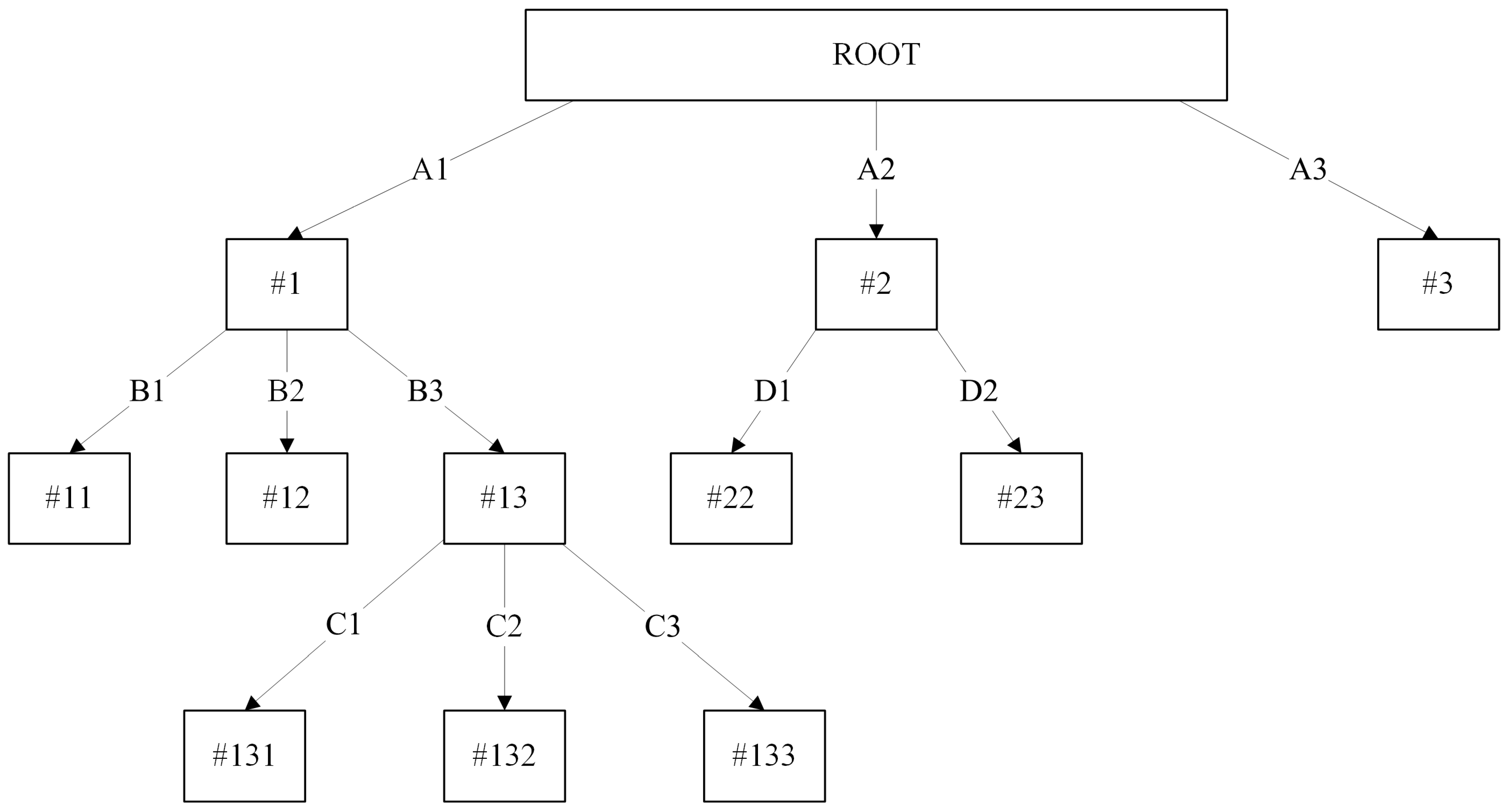
Figure 1. Example of an unpruned decision tree. Numbered labels (e.g., #1, #11, #13, #131) refer to nodes, while alphabetical labels (e.g., A1, B2, C3) indicate attribute splits at each branch.
Electronics 14 03139 g001
Figure 2. Sensitive pruning decision tree. Numbered labels (e.g., #1, #11, #13, #131) refer to nodes, while alphabetical labels (e.g., A1, B2, C3) indicate attribute splits at each branch.
Electronics 14 03139 g002
Figure 3. Limitation of sensitive pruning decision tree. Numbered labels (e.g., #1, #11, #13, #131) refer to nodes, while alphabetical labels (e.g., A1, B2, C3) indicate attribute splits at each branch.
Electronics 14 03139 g003
Figure 4. Limitation of sensitive pruning decision tree. Once node #23 is pruned, node #22 becomes insignificant. Numbered labels (e.g., #1, #11, #13, #131) refer to nodes, while alphabetical labels (e.g., A1, B2, C3) indicate attribute splits at each branch.
Electronics 14 03139 g004
Figure 5. Pessimistic sensitive pruning decision tree. Numbered labels (e.g., #1, #11, #13, #131) refer to nodes, while alphabetical labels (e.g., A1, B2, C3) indicate attribute splits at each branch.
Electronics 14 03139 g005
Figure 6. A sample decision tree model built using IDS data. The root node (PROTOCOL TYPE) represents the network protocol (e.g., TCP or UDP). The internal nodes (RESP_PORT and RESP_IP) denote the response port and response IP address used in the connections. Leaf nodes indicate the predicted class (NORMAL or ANOMALY) with two numbers in parentheses: the total number of instances and the number of misclassified instances.
Electronics 14 03139 g006
Figure 7. Number of pruned nodes (Y1-axis) (represented by bars) and classification accuracy (Y2-axis) (represented by blue dotted lines) according to each of the pruning algorithms (X-axis) in GureKDDCup [Train: 1~6; Test: 7].
Electronics 14 03139 g007
Figure 8. Number of pruned nodes (Y1-axis) (represented by bars) and classification accuracy (Y2-axis) (represented by blue dotted lines) according to each of the pruning algorithms (X-axis) in UNSW-NB15 [Train: 1~3; Test: 4].
Electronics 14 03139 g008
Figure 9. Number of pruned nodes (Y1-axis) (represented by bars) and classification accuracy (Y2-axis) (represented by blue dotted lines) according to each of the pruning algorithms (X-axis) in CIDDS-001 [Train: 1; Test: 2].
Electronics 14 03139 g009
Figure 10. ASCII-sensitive pruned tree model (partial), performance result, and confusion matrix on CIDDS-001.
Electronics 14 03139 g010
Figure 11. Comparison of classification accuracy (%) (Y-axis) according to each classifier (X-axis) in three experimental datasets: GureKDDCup [Train: 1~6; Test: 7], UNSW-SW15 [Train: 1~3; Test: 4], and CIDDS-001 [Train: 1; Test: 2]. The classifiers enclosed in the red box (J48U-SP, J48U-OSP, J48U-PSP, J48P-SP, J48P-OSP, J48P-PSP) represent the proposed pruning algorithms.
Electronics 14 03139 g011
Table 1. Range of private IP addresses.
Starting IPEnding IP
10.0.0.010.255.255.255
172.16.0.0172.31.255.255
192.168.0.0192.168.255.255
Table 2. Summary of experimental datasets.
Dataset#Used InstancesOriginal AttributesDataset#Used Instances
Full GureKDDCup2,759,49448362008 (2016)
Full UNSW-NB152,540,04749 (raw)
48 (processed)
Full UNSW-NB152,540,047
CIDDS-00118,762,253 12 (raw)
16 (processed)
CIDDS-00118,762,253
Table 3. Full GureKDDCup #instances.
Week#Instances
1177,910
2188,790
3288,369
4113,946
5604,303
6951,361
7434,815
total2,759,494
Table 4. Full GureKDDCup distribution.
Training GroupTesting Group
12~7
1~23~7
1~34~7
1~45~7
1~56~7
1~67
Table 5. UNSW-NB15 dataset cleaning.
Attribute Name Original AttributeModified Attribute Value
state-?
service-?
attack_catNanNormal
labelBackdoorsBackdoor
(ALL)Drop
sport/dport-
0xc0a8?
49,320
0x000b11
0x000c12
0x20205321?
0xcc0952,233
The modified value changed to “?”.
Table 6. Full UNSW-NB15 #instances.
Week#Instances
1700,001
2700,001
3700,001
4440,044
total2,540,047
Table 7. Full UNSW-NB15 distribution.
Training GroupTesting Group
12~4
1~23~4
1~34
Table 8. CIDDS-001 Openstack dataset cleaning.
Attribute NameOriginal AttributeModified Attribute Value
Bytes(M)Multiply (Bytes) with 100,000
Flows(ALL)DROP
Attacktype---normal
FlagsAPRSFFlag_A
Flag_P
Flag_R
Flag_S
Flag_F
IP Address
(Src IP Addr/Dst IP Addr)
DNS 1000.1000.1000.1000
EXT_SERVER2000.2000.2000.2000
(Anonymized IP)3000.3000.3000.3000
Table 9. CIDDS-001 Openstack #instances.
Week#Instances
18,451,520
210,310,733
36,349,783
46,175,897
total31,287,933
Table 10. CIDDS-001 Openstack distribution.
Training GroupTesting Group
12
Table 11. Summary of technical implementation for all pruning algorithms.
Algorithm NamePruning TypeTechnical Implementation
J48U-NONo PruneDefault J48 Weka package pruning is disabled.
J48U-SPSingleStandard sensitive pruning as described in Section 3.1 is applied.
J48U-OSPSingleOptimistic sensitive pruning as described in Section 3.2 is applied.
J48U-PSPSinglePessimistic sensitive pruning as described in Section 3.3 is applied.
J48P-NOSingleDefault J48 Weka package pruning is applied.
J48P-SPHybridDefault J48 Weka package pruning and standard sensitive pruning as described in Section 3.1 are applied.
J48P-OSPHybridDefault J48 Weka package pruning and optimistic sensitive pruning as described in Section 3.2 are applied.
J48P-PSPHybridDefault J48 Weka package pruning and pessimistic sensitive pruning as described in Section 3.3 are applied.
J48U-NO No PruneDefault J48 Weka package pruning is disabled.
All of the proposed pruning algorithms follow the J48 Weka package decision tree growing procedure.
Table 12. Classification accuracies for four pruning algorithms in three experimental datasets.
DatasetPerformance Comparison of Four Pruning Algorithms on Classification Accuracy (%), Number of Pruned Nodes, and Number of Nodes in the Final Tree
J48U-NOJ48U-SPJ48U-OSPJ48U-PSP
TrainTestAccuracy
(%)
#Pruned Nodes#Final
Nodes
Accuracy (%)#Pruned Nodes#Final
Nodes
Accuracy (%)#Pruned Nodes#Final
Nodes
Accuracy (%)#Pruned Nodes#Final Nodes
GureKDDCup
12~738.02760109838.029456104238.029456104238.0294108315
1~23~733.19020886433.1782122874233.1782122874233.1782879470
1~34~782.8676052,29682.860915,93836,35882.860915,93836,35882.860952,121175
1~45~788.14490220,36688.130078,233142,13388.130078,233142,13388.1300219,967399
1~56~788.84530471,47288.8410161,785309,68788.8410161,785309,68788.8410471,079393
1~66~799.95220803,21899.8963189,442613,77699.8963189,442613,77699.8963802,599619
UNSW-NB15
12~496.43730854897.1296792775697.1296792775697.129666701878
1~23~496.5973020,41196.7678255017,86196.7678255017,86196.767816,1164295
1~3496.7778038,92897.0410500733,92197.0410500733,92197.041032,7206208
CIDDS-001
1294.2148019,55799.842919,32623199.842919,32623199.842919,422135
Table 13. Classification accuracies for four hybrid pruning algorithms in three experimental datasets.
DatasetPerformance Comparison of Four Hybrid Pruning Algorithms on Classification Accuracy (%), Number of Pruned Nodes, and Number of Nodes in the Final Tree
J48P-NOJ48P-SPJ48P-OSPJ48P-PSP
TrainTestAccuracy
(%)
#Pruned Nodes#Final
Nodes
Accuracy (%)#Pruned Nodes#Final
Nodes
Accuracy (%)#Pruned Nodes#Final
Nodes
Accuracy (%)#Pruned Nodes#Final Nodes
GureKDDCup
12~738.02931093538.02931093538.02931093538.029310935
1~23~733.18085874299033.17865936292833.17865936292833.1786883430
1~34~782.883032,68119,61582.871739,01313,28382.871739,01313,28382.714552,21185
1~45~788.1692117,944102,42288.1503151,73468,63288.1503151,73468,63288.1286220,122244
1~56~788.8412295,568175,90488.8361348,936122,53688.8361348,936122,53688.8363471,255217
1~66~799.9526484,956318,26299.6842553,549249,66999.6842553,549249,66999.8942802,822396
UNSW-NB15
12~496.50794804374497.13515080346897.13515080346897.131871221426
1~23~496.614611,649876296.697712,462794996.697712,462794996.698317,3373074
1~3496.775120,14118,78797.036222,07316,85597.036222,07316,85597.062334,0724856
CIDDS-001
1294.453710,006955199.845919,37817999.845919,37817999.844519,432125
Table 14. Number of unique IP addresses for each IDS dataset.
Dataset#Number of Unique IP Addresses
Original
Source IP
Original
Destination IP
Private
Source IP
Private
Destination IP
Anonymized
Source IP
GureKDDCup848321,01845460229
UNSW-SB154347896
CIDDS-00138790347856
Table 15. Computation time for evaluating the test instances with each pruning algorithm.
DatasetModel Evaluation Computation Time (s)
J48U-NOJ48U-SPJ48U-OSPJ48U-PSPJ48P-NOJ48P-SPJ48P-OSPJ48P-PSP
GureKDDCup *7.076.186.136.355.996.095.915.82
UNSW-NB15 1.301.391.391.441.381.371.431.38
CIDDS-001 57.6014.6215.2414.4954.4115.4414.5813.91
* Train: 1~6, Test: 7; Train: 1~3, Test: 4; Train: 1, Test: 2.
Table 16. Computation time for building the decision tree with each pruning algorithm.
DatasetModel Building Computation Time (s)
J48U-NOJ48U-SPJ48U-OSPJ48U-PSPJ48P-NOJ48P-SPJ48P-OSPJ48P-PSP
GureKDDCup *858.47844.21892.66902.75941.60987.431000.221003.23
UNSW-NB15 716.19726.27800.56840.07772.63806.63810.90826.64
CIDDS-001 426.21432.50462.97505.36547.07525.35536.31531.94
* Train: 1~6, Test: 7; Train: 1~3, Test: 4; Train: 1, Test: 2.
Table 17. Classification accuracies for four pruning algorithms in three experimental datasets with 24-bit (3-octet) IP address truncation and port bilateral classification.
DatasetPerformance Comparison of Four Pruning Algorithms on Classification Accuracy (%), Number of Pruned Nodes, and Number of Nodes in the Final Tree
J48U-NOJ48U-SPJ48U-OSPJ48U-PSP
TrainTestAccuracy
(%)
#Pruned Nodes#Final
Nodes
Accuracy (%)#Pruned Nodes#Final
Nodes
Accuracy (%)#Pruned Nodes#Final
Nodes
Accuracy (%)#Pruned Nodes#Final Nodes
GureKDDCup
12~785.639408185.6394107185.6394107185.63946813
1~23~784.643606084.644065484.644065484.64402931
1~34~787.6357081787.566419961887.566419961887.5664651166
1~45~789.13860205989.1355565149489.1355565149489.13551763296
1~56~792.35140259992.3154593200692.3154593200692.31542206393
1~66~799.90430305799.8395664239399.8395664239399.83952534523
UNSW-NB15
12~496.60750512696.576110511696.576110511696.57615734553
1~23~496.5706011,41096.50341411,39696.50341411,39696.503414369974
1~3496.1983018,93996.74061418,92596.74061418,92596.7406231716,622
CIDDS-001
1289.7284083499.448660323199.448660323199.4486695139
Bold indicates performance improvement compared with the original data in Table 12 and Table 13.
Table 18. Classification accuracies for four hybrid pruning algorithms in three experimental datasets with 24-bit (3-octet) IP address truncation and port bilateral classification.
DatasetPerformance Comparison of Four Hybrid Pruning Algorithms on Classification Accuracy (%), Number of Pruned Nodes, and Number of Nodes in the Final Tree
J48P-NOJ48P-SPJ48P-OSPJ48P-PSP
TrainTestAccuracy
(%)
#Pruned Nodes#Final
Nodes
Accuracy (%)#Pruned Nodes#Final
Nodes
Accuracy (%)#Pruned Nodes#Final
Nodes
Accuracy (%)#Pruned Nodes#Final Nodes
GureKDDCup
12~785.639476585.639476585.639476585.6394765
1~23~784.6445303084.6445332784.6445332784.64453921
1~34~787.628943338487.576246535287.576246535287.4157698119
1~45~788.1952144661388.2147151954088.2147151954088.30481853206
1~56~798.71241467113298.67531469113098.67531469113098.68522304295
1~66~798.78021832122598.76682042101598.76682042101599.85652746311
UNSW-NB15
12~496.64391287383996.61461297382996.61461297382996.614616793447
1~23~496.61203499791196.54373513789796.54373513789796.543740317379
1~3496.2399709711,84296.7874710911,83096.7874710911,83096.7940776711,172
CIDDS-001
1289.764420263299.448472411099.448472411099.449277163
Bold indicates performance improvement compared with the original data in Table 12 and Table 13.
Table 19. Classification accuracies and performance comparison of eight pruning algorithms in three experimental datasets with 24-bit (3-octet) IP address truncation and port bilateral classification.
DatasetPerformance Comparison of Eight Pruning Algorithms on Classification Accuracy and Number of Final Nodes Against Original Dataset and Modified Dataset
J48U-NOJ48U-SPJ48U-OSPJ48U-PSPJ48P-NOJ48P-SPJ48P-OSPJ48P-PSP
TrainTestAccuracy
(%)
#Final NodesAccuracy (%)#Final NodesAccuracy (%)#Final NodesAccuracy (%)#Final NodesAccuracy (%)#Final NodesAccuracy (%)#Final NodesAccuracy (%)#Final NodesAccuracy (%)#Final Nodes
GureKDDCup
12~7+47.61−1017+47.61−971+47.61−971+47.61−2+47.610+47.610+47.610+47.610
1~23~7+51.45−8804+51.47−8688+51.47−8688+51.47−39+51.46−2960+51.47−2901+51.47−2901+51.47−9
1~34~7+4.77−51,479+4.71−35,740+4.71−35,740+4.71−9+4.75−19,231+4.70−12,931+4.70−12,931+4.70+34
1~45~7+0.99−218,307+1.01−140,639+1.01−140,639+1.01−103+0.03−101,809+0.06−68,092+0.06−68,092+0.18−38
1~56~7+3.51−468,873+3.47−307,681+3.47−307,681+3.470+9.87−174,772+9.84−121,406+9.84−121,406+9.85−78
1~66~7−0.05−800,161−0.06−611,383−0.06−611,383−0.06−96−1.17−317,037−0.92−248,654−0.92−248,654−0.04−85
UNSW-NB15
12~4+0.17−3422−0.55−2640−0.55−2640−0.55+2675+0.14+95−0.52+361−0.52+361−0.52+2021
1~23~4−0.03−9001−0.26−6465−0.26−6465−0.26+56790.00−851−0.15−52−0.15−52−0.15+4305
1~34−0.58−19,989−0.30−14,996−0.30−14,996−0.30+10,414−0.54−6945−0.25−5025−0.25−5025−0.27+6316
CIDDS-001
12−4.49−18,723−0.390−0.390−0.39+4−4.69−8919−0.40−69−0.40−69−0.40−62
Bold indicates performance improvement compared with the original data in Table 12 and Table 13.
Table 20. Classification accuracies of ten benchmark machine learning models and proposed sensitive pruning algorithms in three experimental datasets.
Machine
Learning Model
Classification Accuracies for Each Dataset
GureKDDCup *UNSW-NB15 CIDDS-001
ZeroR47.284579.798882.5870
Random Tree99.388079.165778.9227
REPtree97.650782.095971.5996
Decision Stump95.725191.612085.5956
Adaboost95.725191.612096.8684
Bayesnet98.366294.347285.4093
Naïve Bayes87.499788.963156.3338
Random Forest99.516196.664984.6270
SMO83.407494.096775.1466
J48U-NO99.952296.777894.2148
J48U-SP99.896397.041099.8429
J48U-OSP99.896397.041099.8429
J48U-PSP99.896397.041099.8429
J48P-NO99.952696.775194.4537
J48P-SP99.684297.036299.8459
J48P-OSP99.684297.036299.8459
J48P-PSP99.894297.062399.8445
* Train: 1~6, Test: 7; Train: 1~3, Test: 4; Train: 1, Test: 2. Bold indicates the best model performance for each dataset.
Disclaimer/Publisher’s Note: The statements, opinions and data contained in all publications are solely those of the individual author(s) and contributor(s) and not of MDPI and/or the editor(s). MDPI and/or the editor(s) disclaim responsibility for any injury to people or property resulting from any ideas, methods, instructions or products referred to in the content.