1. Introduction
Synaptic connections are vital for transmitting information between neurons. Prior research has confirmed the existence of synaptic crosstalk in biological synapses [
1], which significantly impacts brain activity and function. However, this phenomenon is rarely taken into account in neural network studies. The interactions between neurotransmitters at synaptic sites are crucial for maintaining normal brain function, especially in terms of behavioral cognition and synaptic plasticity [
2]. By emulating the interactions between neurons and synapses observed in the brain [
3], researchers can obtain a more profound understanding of brain mechanisms and apply these insights to the development of advanced neural network models.
The memristor is a nonlinear circuit element whose resistance can vary in response to changes in current and voltage, which possesses a memory property, and is considered the fourth fundamental circuit component, in addition to resistance, capacitance, and inductance [
4]. By regulating the voltage applied across the memristor, its resistance can be adjusted in a nonlinear and continuous manner. This resistance change is retained even after power is removed, corresponding, respectively, to the plasticity [
5] and memorability [
6] of synaptic weights, respectively [
7]. In recent years, memristive neural networks have gained increasing prevalence [
8,
9,
10,
11]. Among them, the Hopfield neural network (HNN) [
12] has emerged as a prominent artificial neural network, attracting substantial interest from scholars [
13,
14]. The ability of the HNN to stimulate complex dynamical behaviors observed in the brain, particularly chaotic phenomena, is largely due to its strong nonlinearity and flexible algebraic formulations. Leveraging the distinct advantages of memristors, researchers have developed memristive Hopfield neural networks (MHNNs) [
13,
14,
15,
16,
17], which have been widely applied in diverse research areas such as associative memory, image processing, and combinatorial optimization [
16,
17,
18,
19,
20].
Conducting circuit experiments is a common approach for analyzing and verifying dynamic behaviors of neurons and neural networks. However, due to the impact of fabrication processes and environmental variations, transistor mismatch in practical circuits remains difficult to eliminate. Field Programmable Gate Arrays (FPGAs) are primarily based on digital logic design, and digital circuits require less stringent signal accuracy than analog circuits. Signals in digital circuits usually have a large noise tolerance, so some small parameter deviations are unlikely to cause significant changes in dynamics. In addition, compared to traditional analog circuits, FPGAs are usually manufactured using advanced manufacturing processes which have stricter control of component parameters during the manufacturing process, thus reducing the possibility of mismatches. To further uncover the mechanisms underlying complex phenomena in neural network computation and to replicate the dynamic behavior of neuronal models, the development of efficient brain-inspired computing hardware is essential [
21]. Among various digital design platforms, FPGA is distinguished by its high flexibility, real-time performance, and portability, making it well suited to the diverse requirements of memristive neural network systems. H. Lin et al. verified the physical realizability of memristive neural networks and demonstrated a medical image encryption design using FPGA [
22]. HNN is also widely used in industrial applications [
21,
22,
23,
24]. Q. Lai et al. incorporated the amnesia model into HNN, modeled the synaptic components with memristive properties, proposed a novel high-dimensional HNN structure with multiple double-scroll chaotic attractors, and applied it to a 3D image encryption scheme [
25].
Existing studies on the chaotic dynamics of memristive neurons and neural networks explore a variety of models such as memristive self-synaptic neurons and synaptic coupled networks, and present rich nonlinear phenomena such as multistability and extreme multistability and their applications in areas such as secure communications. In this paper, a MHNN with synaptic crosstalk is proposed, and the physical feasibility of the model is verified by FPGA implementation and simulation circuits, and finally, a dynamic key image encryption scheme based on chaotic sequences is developed.
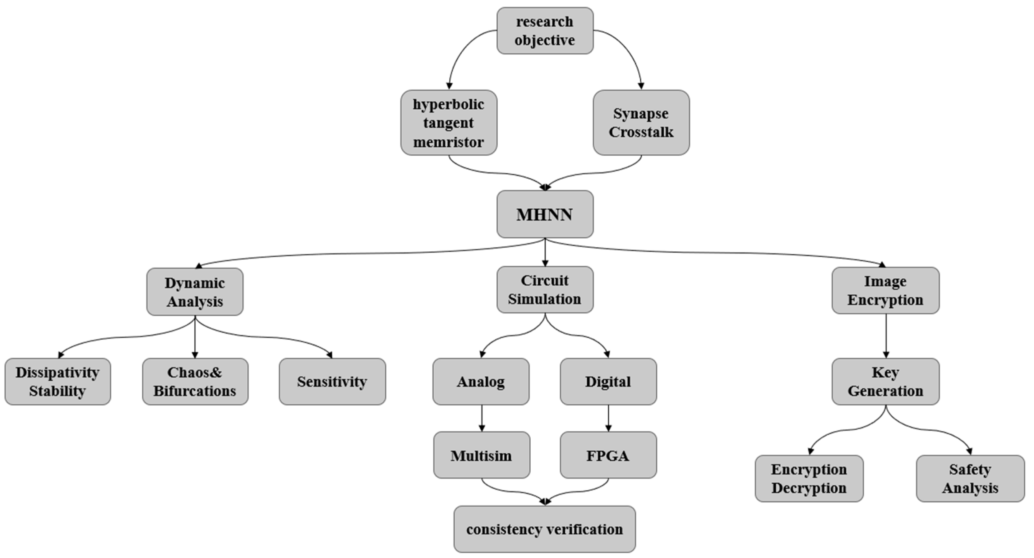
Based on the above-mentioned research, this study aims to make following contributions, which are shown in
Figure 1:
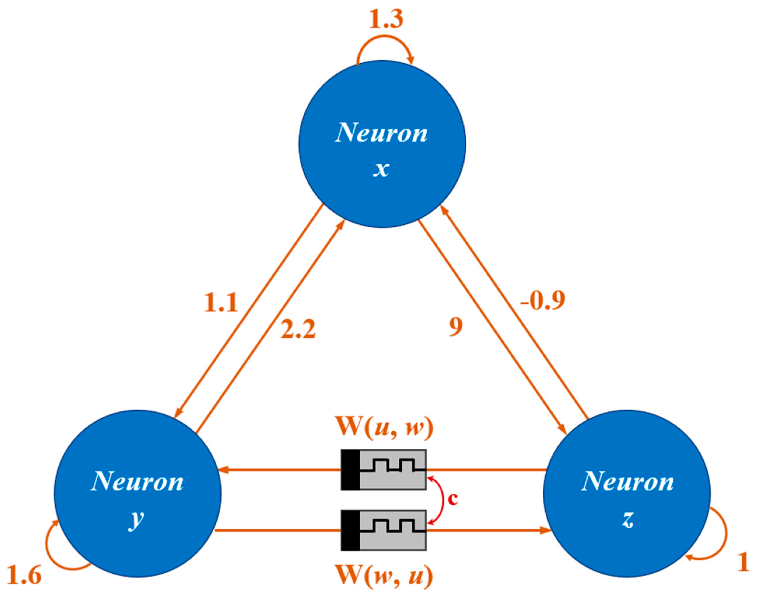
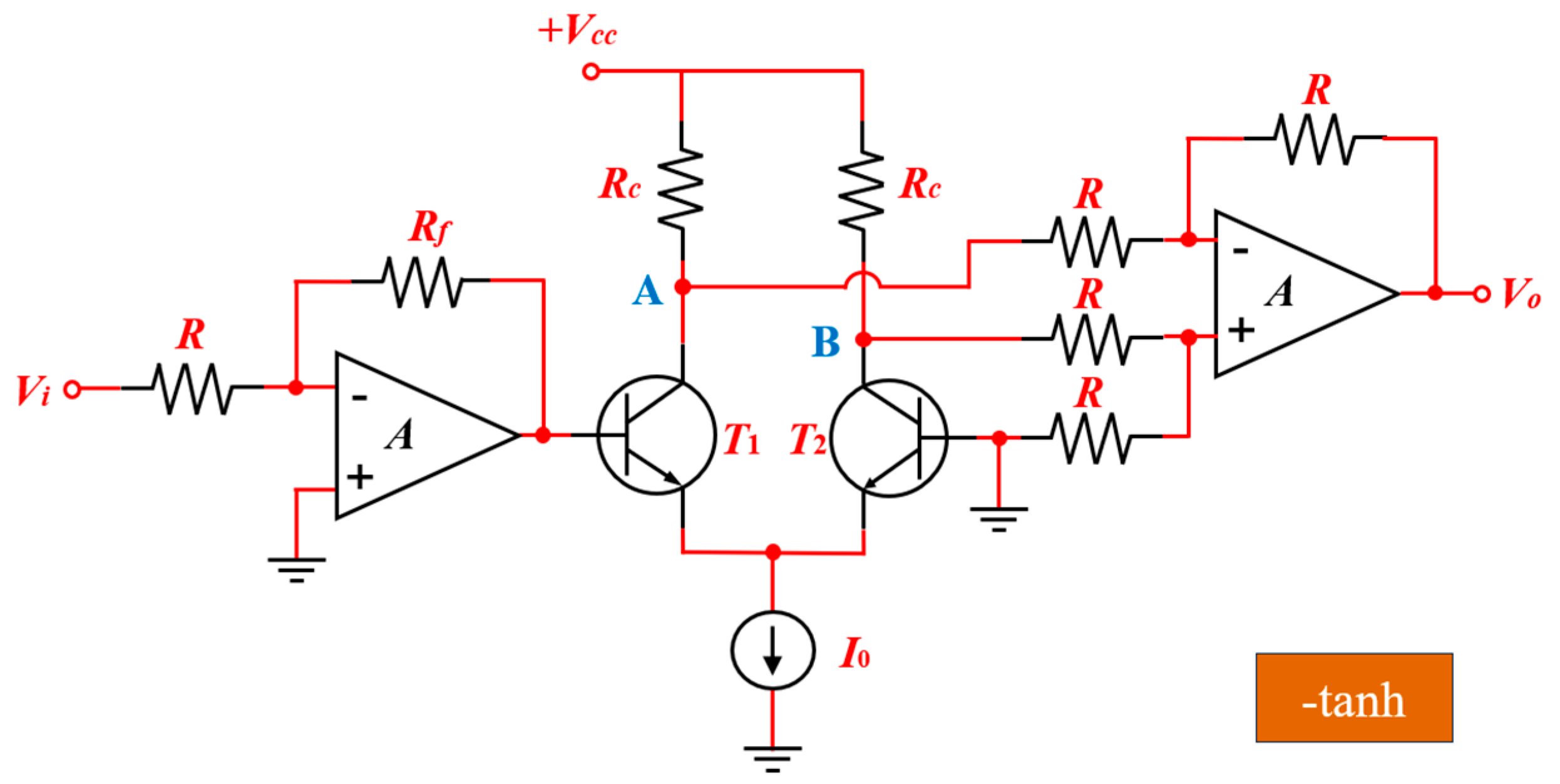
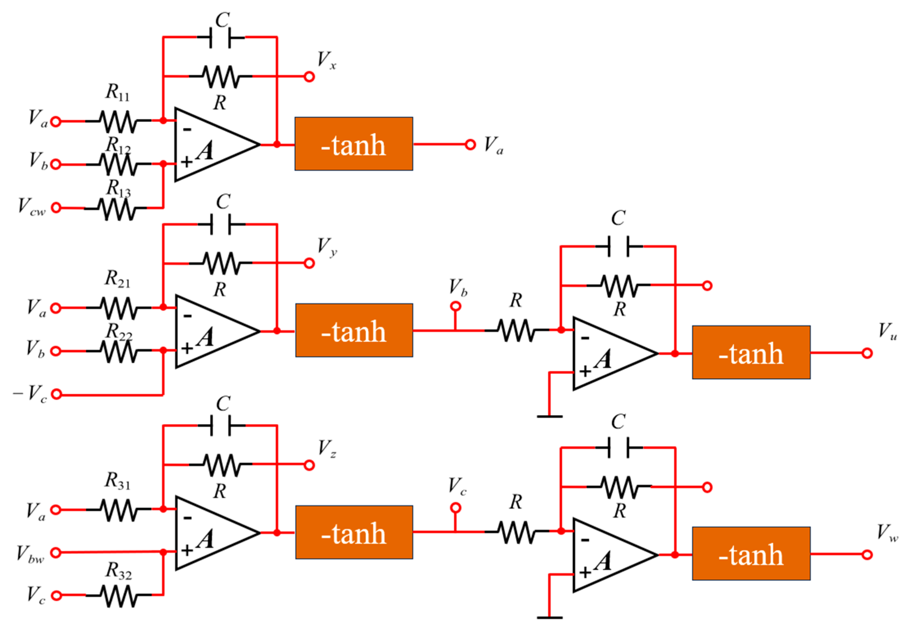
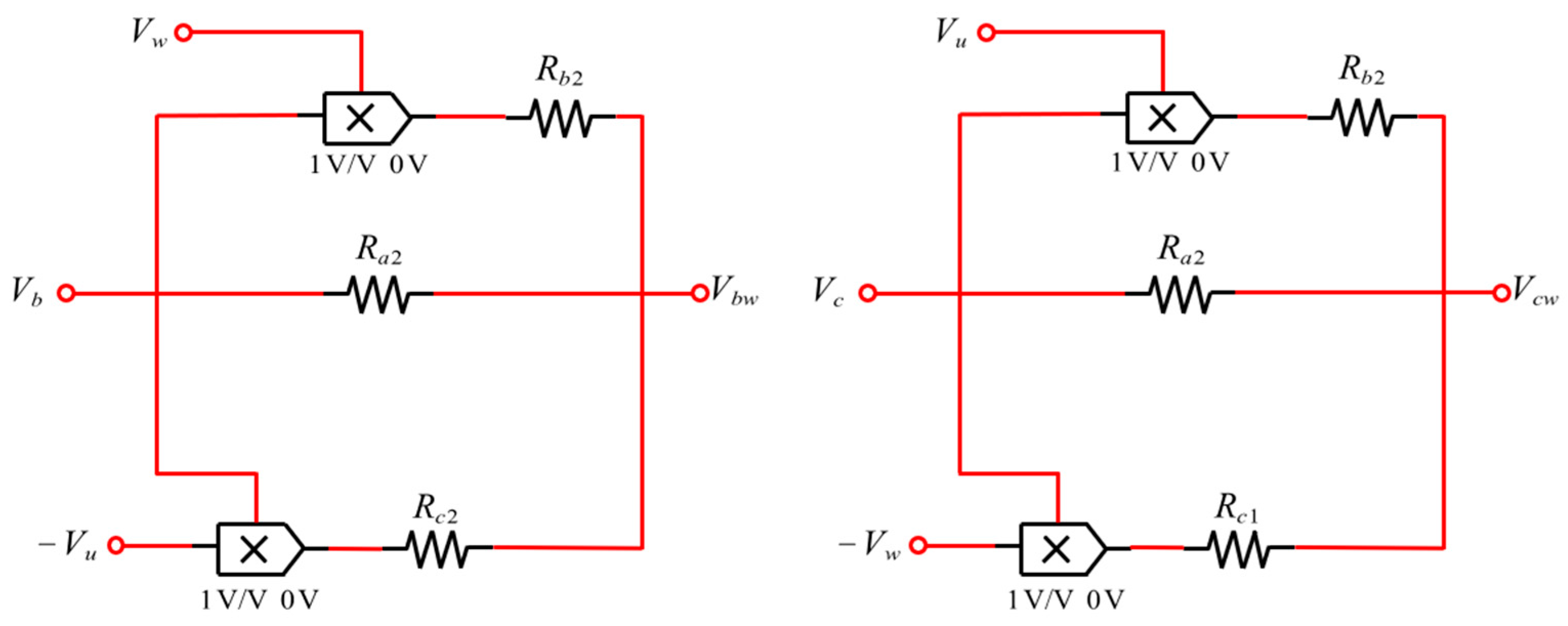
(1) A memristor model based on the hyperbolic tangent function is proposed to simulate the activation function of neurons. Utilizing this memristor model, a three-neuron HNN incorporating synaptic crosstalk is constructed by coupling two memristors.
(2) The complex nonlinear dynamical behavior of the memristor-based HNN is analyzed using multiple methods. The results reveal that, as system parameters vary, the network displays a wide range of dynamic behaviors, such as period-doubling bifurcations, chaotic states, and periodic oscillations.
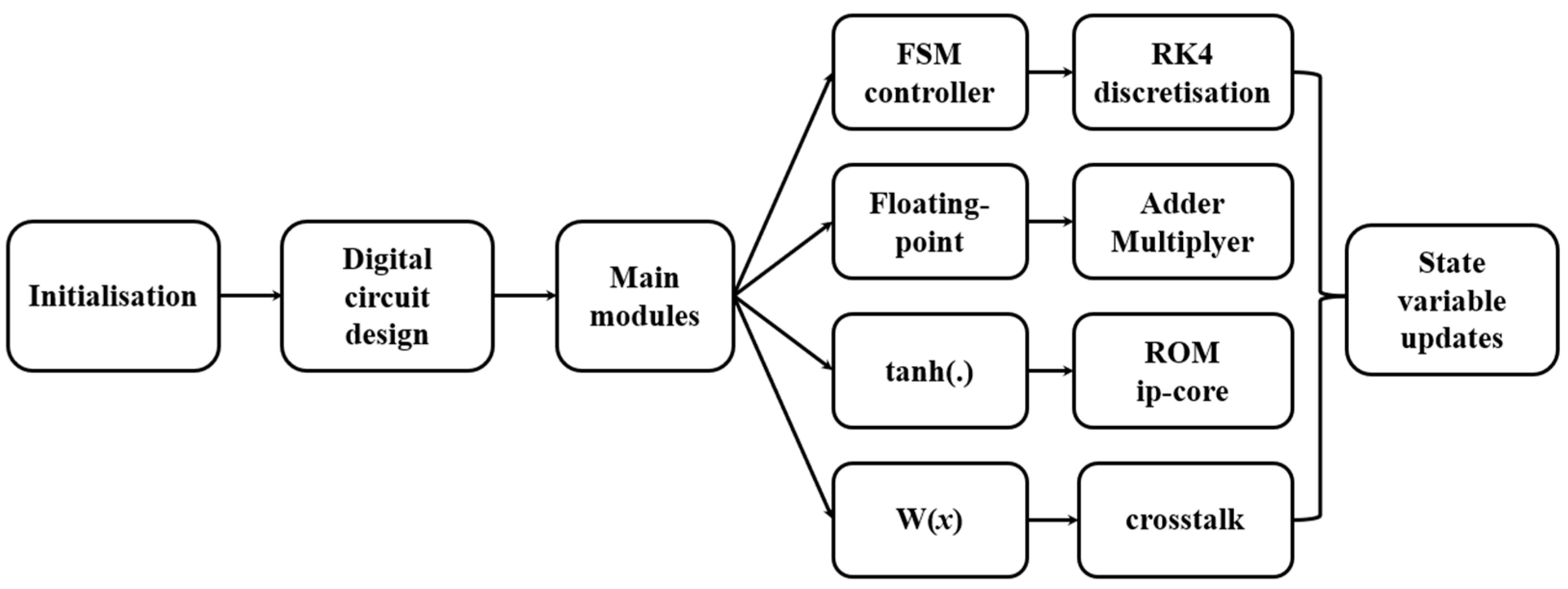
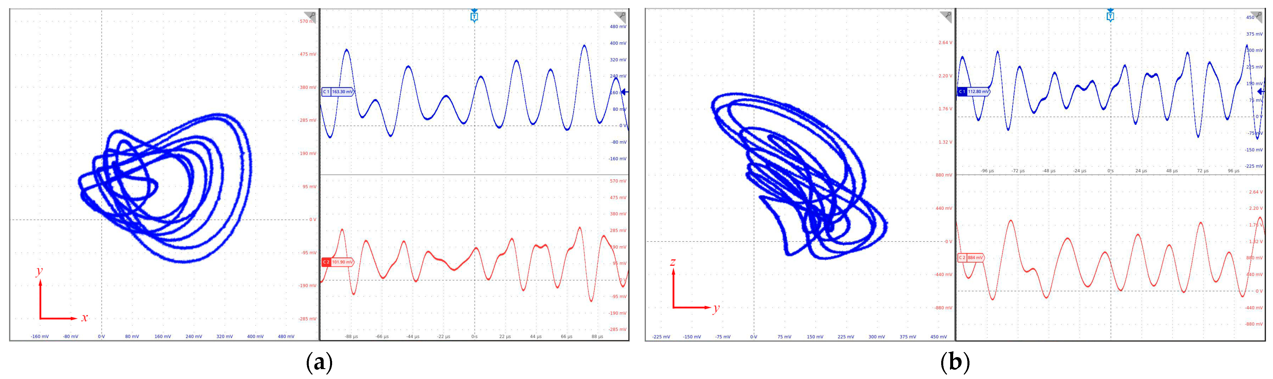
(3) The physical realizability of the MHNN is validated through both circuit simulation and FPGA implementation. First, a circuit module capable of realizing the MHNN is designed, and its output is verified against the theoretical model using Multisim simulation, ensuring the reproducibility of the system’s dynamical behavior. Subsequently, the FPGA implementation of the MHNN further demonstrates its potential for simulating complex dynamical behaviors and for real-world applications.
(4) A novel image encryption approach utilizing a five-dimensional chaotic system and a dynamic key generation mechanism is presented. The chaotic system is iterated via the Runge–Kutta-4th (RK4) method to generate a key matrix that is highly correlated with the pixel positions of the original image. Additionally, image encryption and decryption are accomplished through exclusive OR (XOR) operations. Experimental findings demonstrate that this method effectively disrupts the statistical properties of the original image, and the histogram of the encrypted image displays a uniform distribution.
In conclusion, dynamical analysis establishes the MHNN’s nonlinear behaviors as a theoretical foundation while circuit simulation and image encryption test these behaviors in a real-world task requiring both chaos and hardware efficiency.
3. Dynamic Analysis of MHNN
This section focuses exclusively on characterizing crosstalk-driven dynamics. In this part, a range of fundamental dynamic analysis techniques are applied to investigate the complex nonlinear chaotic behavior of the MHNN in this study. These methods include dissipativity evaluation, equilibrium point assessment, phase space visualization, bifurcation analysis, Lyapunov exponent computation, and time series inspection.
3.1. Dissipativity Analysis
Based on the Lyapunov stability criterion [
26], a five-variable Lyapunov function can be constructed as follows:
The partial derivative of time for Equation (6) is
where
For all
, there is
, so it can be obtained that
Let
. According to Equation (9), Equation (8) satisfies
Let us suppose that all the state variables satisfy
. A sufficiently large domain
is selected, and in a limited domain, it is always true that
. It is required that
where
is a positive constant.
Since
, it is obvious that
Based on Equation (12), it can be concluded that the confined domain of the solutions in Equation (5) can be given as
From the analysis above, the system is bounded and has the possibility to generate chaotic behaviors.
3.2. Equilibria Analysis
Setting the left-hand side of Equation (5) to zero yields the following result:
Hence, the equilibrium point of Equation (5) corresponds to the solution of Equation (14), which can be reformulated as
where the equilibria of HNN are the intersections of surfaces of
,
, and
.
Let
,
, and
be equal to zero, and setting
,
and
, the three surfaces are shown in
Figure 5. As can be visualized from the figure, there are two intersections in total, which are equilibriums of the system within the given parameters.
By linearizing Equation (5) at the equilibrium point, the Jacobian matrix can be expressed as
where
.
The characteristic equation at
can be formulated as
Based on the partitioned matrix determinant equations, Equation (17) can be calculated as
where
Therefore, the coefficients in Equation (17) are
According to the Routh–Hurwitz stability criterion, the Routh Array can be given as [
25]
When , , so the system is unstable in the given condition and it can produce chaotic or hyperchaotic phenomena.
Based on the analysis above, the eigenvalues and stabilities of other equilibrium points within different synaptic crosstalk strengths are shown in
Table 1, which demonstrate no significant effect on the stability of the system within a certain range.
3.3. Dynamic Behaviors
When
, the representative Lyapunov exponents are
Since the maximum Lyapunov exponent , the system can produce chaos.
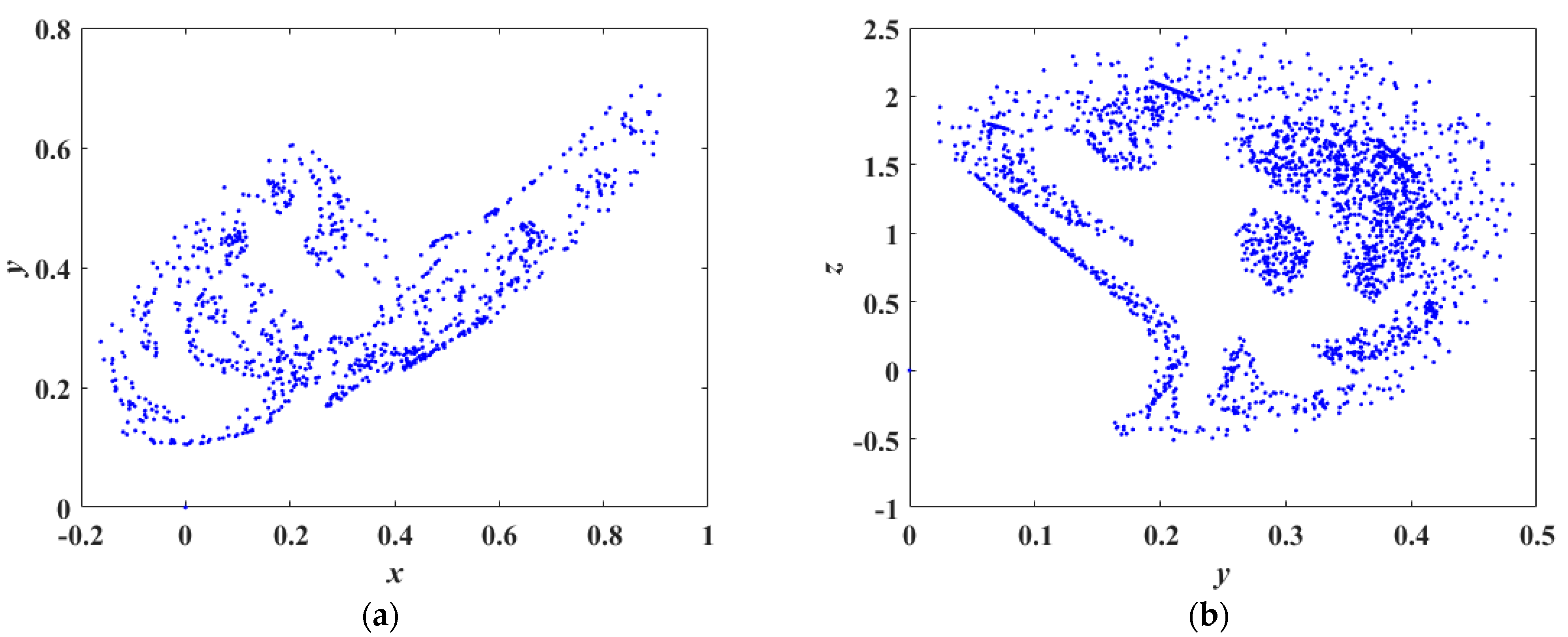
By numerically simulating the time evolution of the system, the trajectories of the state variables
can be plotted and the system’s dynamic behaviors can be examined. For Equations (3) and (5), the parameters are set as
,
and
with the initial conditions defined as
. The chaotic behaviors of the system under the given conditions are, respectively, illustrated in the subplots of
Figure 6.
The Poincaré map is a method commonly used to verify the presence of chaotic phenomena. It reveals the dynamic characteristics of a system by selecting a specific hyperplane in the phase space and recording the state values each time the system trajectory intersects this hyperplane.
Figure 7 presents the Poincaré map in the
x-y-z space with cross-sections defined by
and
, in which it can be seen that the points on the cross-section form a piece of discrete two-dimensional shapes, which indicates the existence of chaotic attractors.
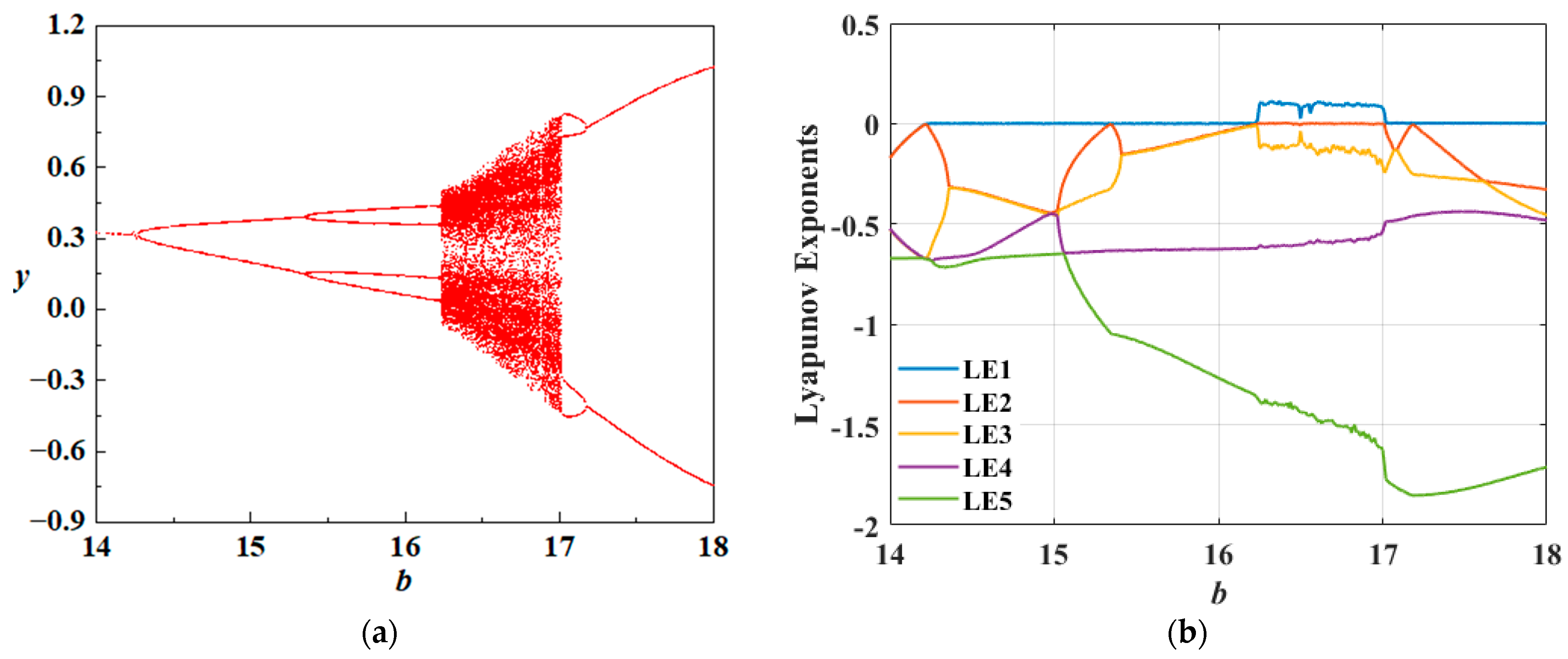
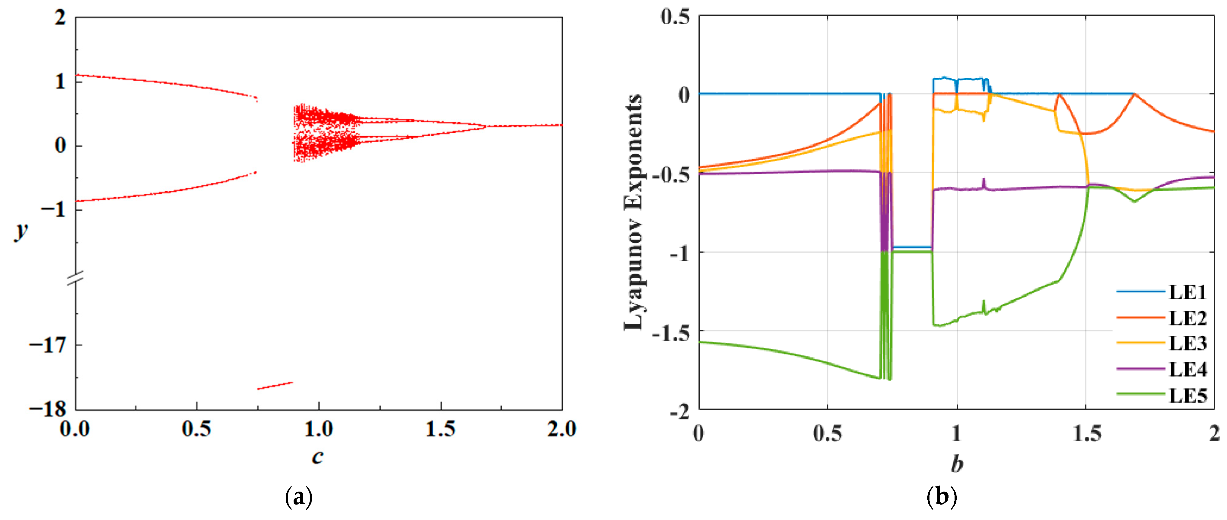
3.4. Memristive Parameter b-Associated Dynamics
The internal memristive parameter
is selected as the bifurcation parameter of the system, and numerical simulations are performed in MATLAB 2023b using the RK4 method with a step size
. When
is selected as the sole bifurcation parameter, with
and
held constant, the corresponding single-parameter bifurcation diagram of the state variable
and the associated Lyapunov exponents can be generated to characterize the system’s dynamic behavior. The initial state is set as
. To accurately track the system’s evolution over time, suitable simulation configurations are employed. For the bifurcation diagram, the start time, time step size, and end time are configured to 500 s, 0.01 s, and 2500 s, respectively. For the computation of the finite-time Lyapunov exponents, the time step and end time are set to 0.01 s and 10,000 s, respectively. The system’s dynamic behaviors as the parameter increases from 14 to 18 are depicted in
Figure 8.
Figure 8 presents the bifurcation diagram in the
y phase along with the corresponding Lyapunov exponent spectrum of the system. It can be observed that the dynamic behaviors revealed by both methods exhibit consistent trends. Specifically, as the parameter
increases within the interval
, the system maintains a stable fixed point. When
reaches 14.26, the first periodic bifurcation occurs, during which the system undergoes a supercritical Andronov–Hopf bifurcation and transitions into a period-1 oscillatory state. As
b continues to increase, the system experiences a second bifurcation at
, entering a period-2 oscillatory state. Subsequently, within the interval
, the number of branches in the bifurcation diagram increases significantly and becomes densely distributed, indicating that the system gradually transitions from a quasi-periodic state to a chaotic state. Finally, at
, the system undergoes a sudden transition from chaos back to a periodic oscillatory state.
To more effectively reveal the coexisting symmetric behaviors, the phase portraits of the HNN under parameter
b and the time-domain waveforms are drawn in
x-y phase, as illustrated in
Figure 9.
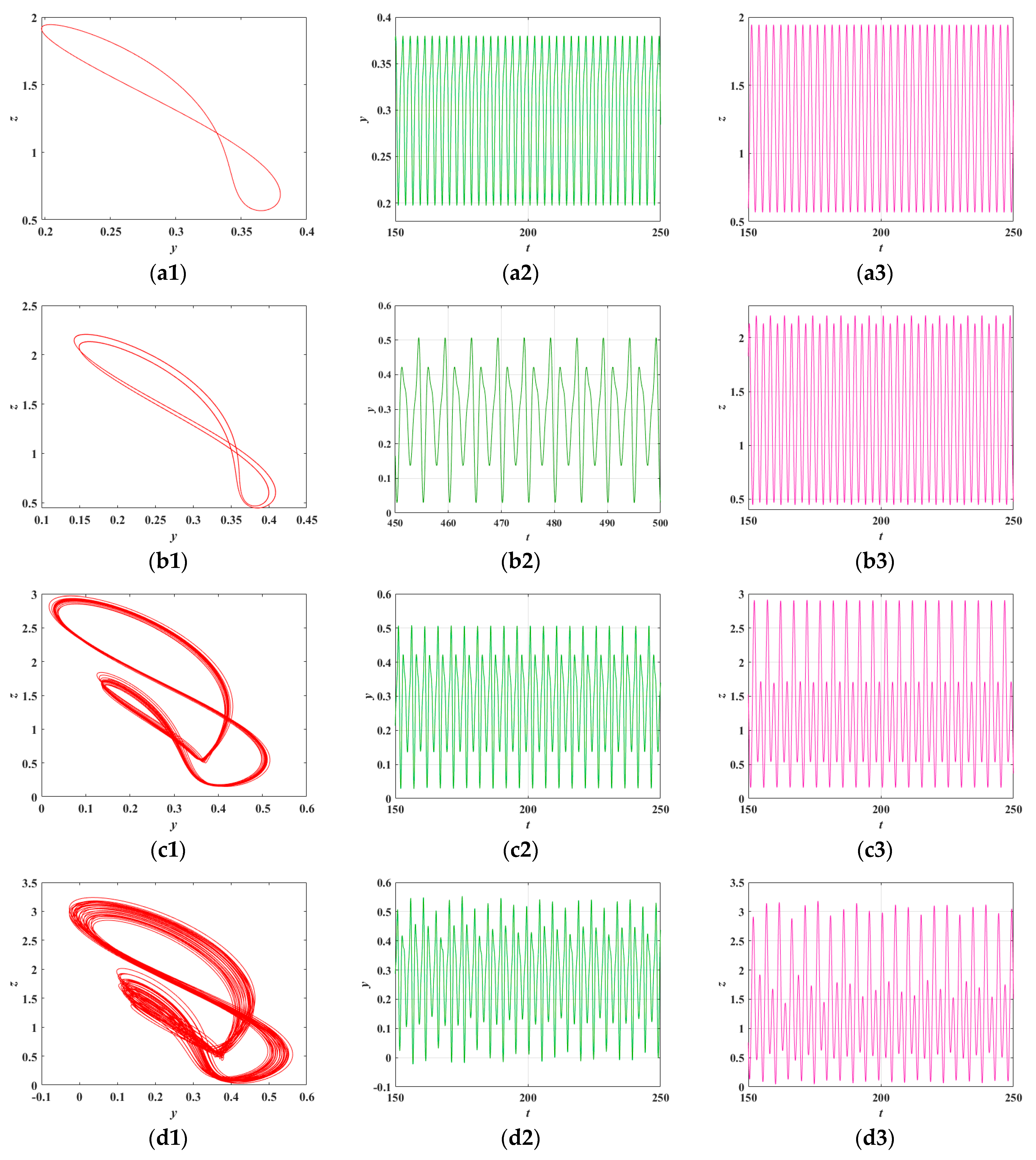
The results illustrate the nonlinear dynamical evolution of the system as the parameter increases. Initially, at , the system exhibits periodic oscillations, suggesting that the magnetic field has minimal influence on the neurons and that the system maintains the intrinsic periodic spiking behavior of neuronal activity. As increases to 16, the system undergoes a period-2 bifurcation. The previously stable limit cycle splits into two distinct cycles, resulting in alternating behavior between two closed loops in the phase portrait. In this state, the neurons display period-2 bursting oscillations. With a further increase in to 16.2, the system undergoes additional bifurcations and transitions into a quasi-periodic state. The corresponding phase portrait reveals densely packed oscillatory patterns, indicating that the system is no longer constrained to a simple limit cycle but instead exhibits more intricate and irregular dynamics. This evolution also implies a growing degree of coupling between the magnetic field and the neural system. As continues to increase, the system reaches a chaotic regime at , characterized by hyperchaotic bursting behavior in the neurons. Remarkably, a slight increase to results in a rapid transition back to a period-2 oscillatory state, further highlighting the system’s sensitivity to parameter changes and the richness of its nonlinear dynamical responses.
Based on the combined analysis of the bifurcation diagram, phase portraits, and waveform evolution, it can be concluded that the system is capable of generating both periodic and chaotic behaviors. This confirms that the system exhibits rich and complex dynamical characteristics.
3.5. Memristive Crosstalk Strength c-Associated Dynamics
Here, with parameters set as
and
, the bifurcation behavior of the HNN within the interval
is illustrated in
Figure 10.
When the crosstalk intensity is low, the highest Lyapunov exponent is negative, and the system exhibits periodic oscillations. As increases within the interval , the Lyapunov exponents undergo a sudden change, and the maximum value remains below zero, indicating that the system enters a stable fixed-point state. When , the maximum Lyapunov exponent and the system begins to generate sustained periodic oscillations. As further increases to 1.17, the system undergoes a subcritical Hopf bifurcation, transitioning into a period-2 bursting oscillatory state. In the interval , the system exhibits periodic oscillations once again, and when , the system stabilizes.
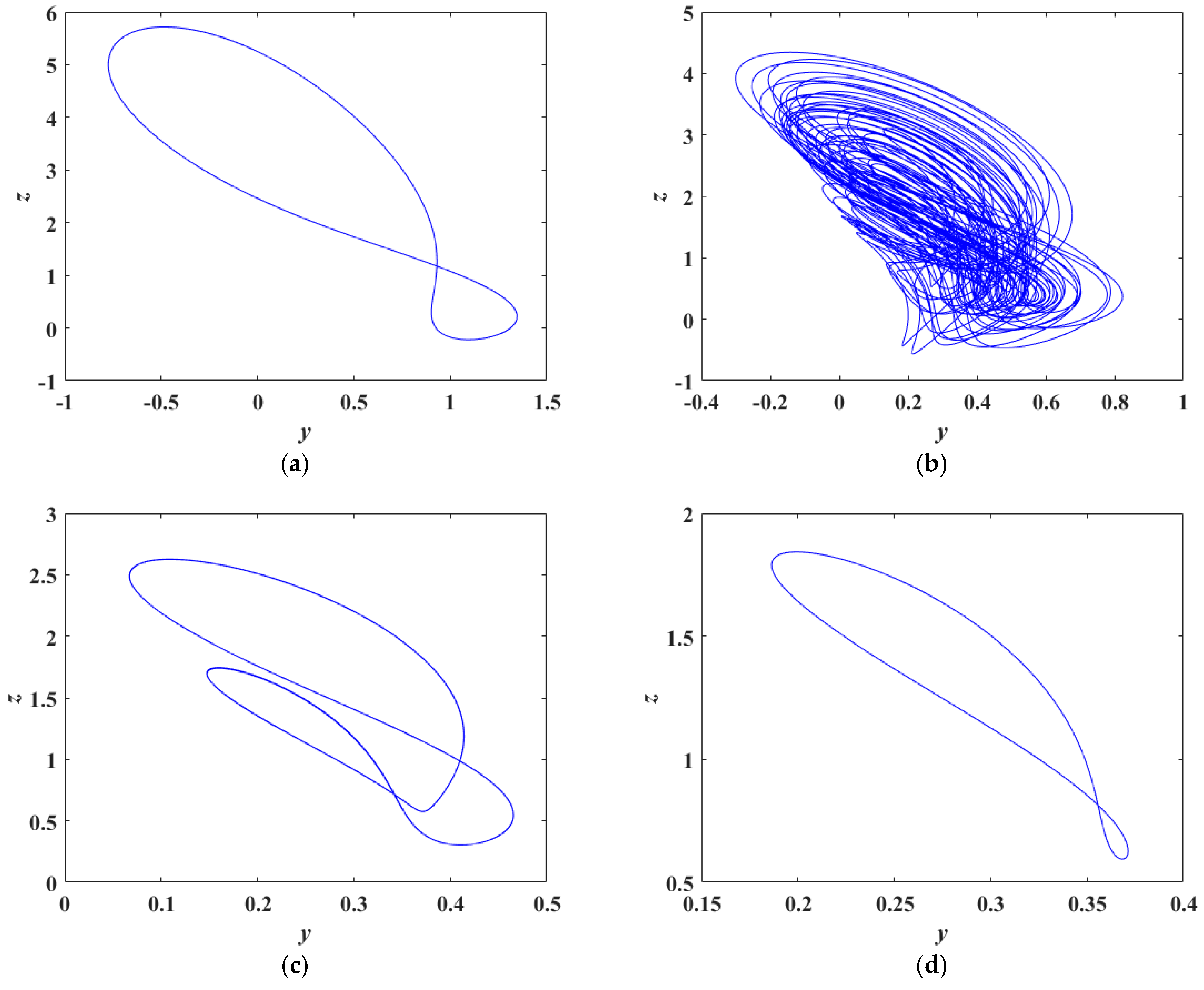
By setting
and
, the HNN exhibits different attractors depending on the value of the crosstalk parameter
, as illustrated in
Figure 11. When the crosstalk strength is low, neurons display periodic spike firing, suggesting that external stimuli have limited influence on neuronal dynamics. As the crosstalk intensity increases, the firing pattern changes, giving rise to chaotic spike firing or cluster firing behaviors. When the crosstalk intensity reaches a high level, the firing activity of the neurons stabilizes and the overall system becomes dynamically stable.
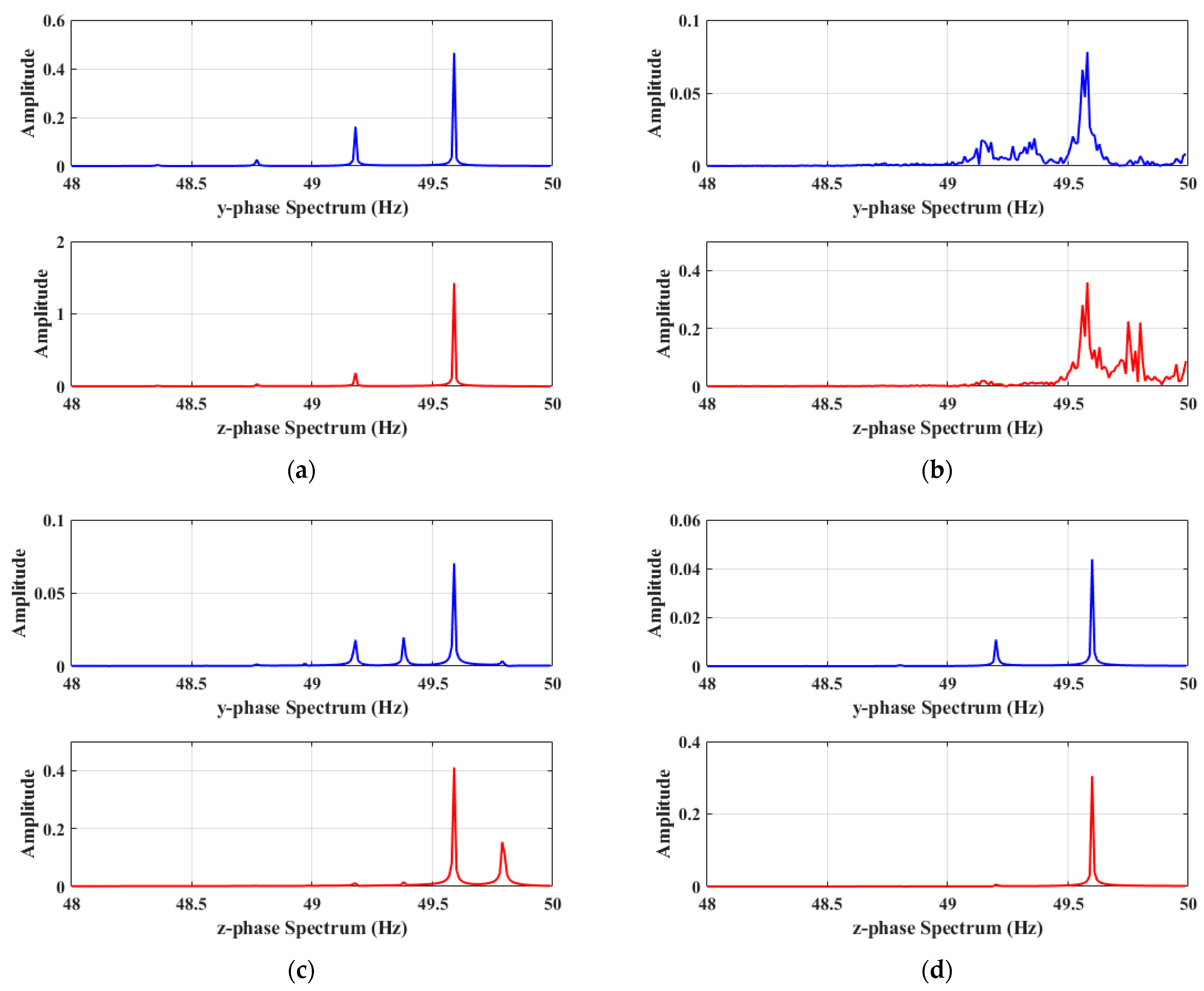
To examine the signal spectrum under various crosstalk strengths, the Fast Fourier Transform (FFT) algorithm is employed. The frequency-domain signal characteristics of the system for different values of the parameter
, corresponding to
,
,
and
, are presented in
Figure 12. Each subfigure contains the amplitude response curves of the
y phase and
z phase. The analysis results show that for all values of the parameter
, the amplitude responses of both
y phase and
z phase show significant peaks in the mid-frequency band (about 49.6 Hz), indicating that the system has a strong response at this frequency. However, with the increase in parameter
, the amplitude response of
y phase and
z phase decreased. This indicates that the parameter
has a significant effect on the frequency response characteristics of the system, especially on the response strength in the middle frequency band.
5. Image Encryption Application
Image encryption plays a vital role in the realm of information security. Traditional methods, such as the Arnold transform and Logistic mapping, often suffer from limitations including a small key space and the tendency to preserve statistical features of the original image. In contrast, chaotic systems exhibit extreme sensitivity to initial conditions, where even slight changes can lead to entirely different key matrices. Moreover, the ergodicity of chaotic systems ensures a random distribution of key matrix elements. Additionally, since the elements of the key matrix are strongly correlated with pixel positions, the unpredictability and security of the encryption process are significantly enhanced.
Here, we utilize the MHNN’s chaos verified in
Section 3 and
Section 4, where encryption performance is assessed via sensitivity of the key. In this study, a grayscale image is used as the encryption target, and the MHNN serves as the underlying chaotic model. The initial conditions are set to (0.01, 0.01, 0.01, 0, 0), with internal memristor parameters configured as
and synaptic crosstalk
. Under these conditions, chaotic sequences are generated and subsequently processed with the original image to produce the encrypted image.
The key generation algorithm is based on the dynamics of high-dimensional chaotic systems. By numerically solving the chaotic equations, a key matrix that is strongly correlated with the pixel positions of the image is generated, as illustrated in
Figure 19.
The specific steps of the algorithm are as follows:
(1) Define the dynamical equations of the five-dimensional chaotic system as given in Equation (5), and numerically solve them using the RK4 method with a step size of .
(2) Initialize the variables as (0.01, 0.01, 0.01, 0, 0). For each pixel
in the image, iterate the chaotic system
times to obtain the chaotic variables
x and
y. These variables are then mapped to the integer range [0, 255] and used to compute the key matrix
K, which can be expressed as
The encryption process is implemented based on the key matrix generated in Equation (26). When encrypting, each pixel of the plaintext
is subjected to a pixel-wise XOR operation with the corresponding element of the key matrix
, which can be expressed as
where
C is the ciphertext image. The pixel values of the ciphertext image
C are uniformly distributed shown in
Figure 20, effectively concealing the information of the original image.
When it comes to the decryption process, the same key matrix
K is used to perform pixel-wise XOR operations on the ciphertext image
C, recovering the original image by
where
P’ is the decrypted image. Due to the reversibility of the XOR operation, the decrypted image
P’ is identical to the original image
P, ensuring lossless recovery of the information.
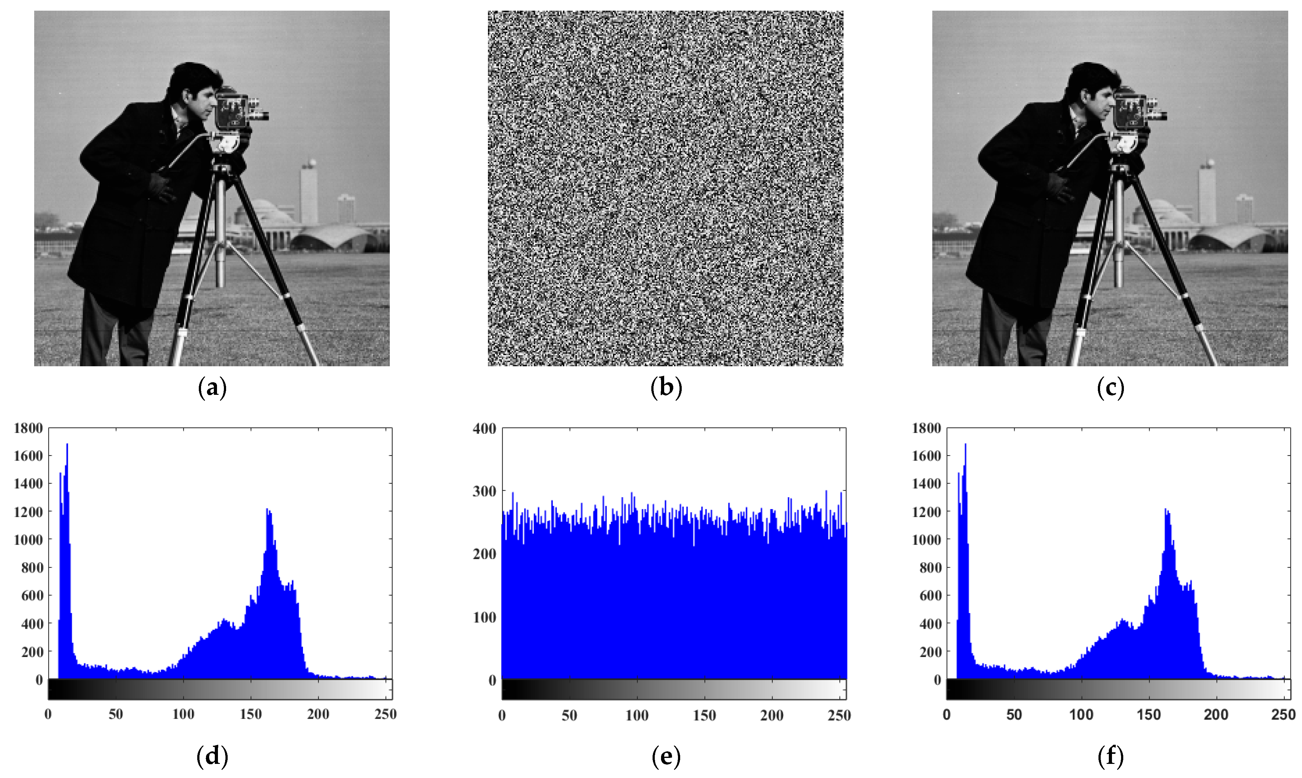
The histogram of the original image shows a highly uneven distribution, featuring distinct variations in sparsity and density, a broad dynamic range, and sharp peaks. In contrast, the histogram of the encrypted image exhibits a uniform distribution, with no significant spikes and a much narrower variation range, indicating that the encryption algorithm effectively disrupts the statistical features of the original image.
Key sensitivity is a vital metric for assessing the security performance of an encryption system. It is widely acknowledged that key sensitivity that satisfies the avalanche principle meets standard security requirements. Bit change rate refers to the ratio of the number of bits of the encrypted image’s octet binary value per pixel that change to the total number of bits when a small perturbation is applied to the system parameters. The avalanche principle states that an extremely small change in the key should result in a random alteration of each bit in the ciphertext sequence, with the bit change rate approaching 50%. In this study, slight perturbations were introduced to the parameters of the memristive neural network, and the corresponding changes in the encrypted ciphertext were observed. Specifically, the parameters
,
, and
were individually varied by 10
−8. The results presented in
Table 4 clearly exhibit the avalanche effect, demonstrating strong key sensitivity and dependence. These findings further confirm the inherent sensitivity of chaotic systems to initial conditions.
The experimental results demonstrate that the proposed algorithm effectively disrupts the statistical features of the original image. In addition, the histogram of the ciphertext image exhibits a uniform distribution, and the decrypted image is completely identical to the original image.
6. Conclusions
This research proposes a novel MHNN that incorporates synaptic crosstalk, utilizing hyperbolic tangent memristors to simulate complex neuronal dynamics. The constructed three-neuron MHNN displays a wide range of nonlinear behaviors, including chaotic states, periodic oscillations, and bifurcations, as uncovered through comprehensive dynamical analyses. Methods such as Lyapunov exponent analysis, bifurcation diagrams, and phase portraits illustrate the system’s sensitivity to internal parameters, particularly the memristive parameter b and the crosstalk strength c. The observed transitions between stable and chaotic regimes underscore the model’s potential for applications that demand adaptability and dynamic response.
The feasibility of the proposed MHNN is further validated through hardware implementation. Circuit simulations in Multisim and FPGA-based realizations confirm the reproducibility of the theoretical dynamics. The integration of hyperbolic tangent memristors into the neural network enhances biological plausibility while bridging the gap to artificial models, thereby demonstrating the practical potential of memristive systems in neuromorphic computing. Moreover, the application of the MHNN to image encryption proves effective in generating position-dependent key matrices with uniform pixel distribution, offering strong resistance to statistical attacks. The high sensitivity of the encryption scheme to initial conditions and parameter variations further underscores its robustness for real-world security applications.
Overall, this work advances the understanding of memristive neural networks by integrating synaptic crosstalk and providing a comprehensive framework for their modeling, analysis, and implementation. Nevertheless, there remains ample room for algorithmic refinement. In future research, the exploration of memristive synapses in chaotic HNN is expected to extend to areas such as intelligent control, artificial intelligence, and the Internet of Things, potentially establishing memristive computing as a core technology in next-generation intelligent systems.


