Article

An Active Learning Didactic Proposal with Human-Computer Interaction in Engineering Education: A Direct Current Motor Case Study

by
Alejandro Said
1,
Luis C. Félix-Herrán
2,*,
Yasser A. Davizón
3,
Carlos Hernandez-Santos
4,
Rogelio Soto
5 and
Ricardo A. Ramírez-Mendoza
1
1
Tecnologico de Monterrey, School of Engineering and Sciences, Ave. Eugenio Garza Sada 2501, Monterrey 64849, Mexico
2
Tecnologico de Monterrey, School of Engineering and Sciences, Blvd. Enrique Mazón López 965, Hermosillo 83000, Mexico
3
Department of Information Technology, Universidad Politécnica del Mar y la Sierra, Potrerillos del Norote, Tayoltita 82740, Mexico
4
Tecnológico Nacional de México/IT de Nuevo León, Mexico, Av. Eloy Cavazos 2001, Guadalupe, Nuevo León 67170, Mexico
5
Electrical and Computer Engineering Department, University of Texas Rio Grande Valley, 1 West University Blvd., Brownsville, TX 78520, USA
*
Author to whom correspondence should be addressed.
Electronics 2022, 11(7), 1059; https://doi.org/10.3390/electronics11071059
Submission received: 3 March 2022 / Revised: 17 March 2022 / Accepted: 21 March 2022 / Published: 28 March 2022
(This article belongs to the Special Issue Electronic Devices and Technology for Educational Applications)

Abstract

:
Engineering education requires learning strategies to engage students and improve the development of disciplinary and transversal competencies. Additionally, as economic resources are generally limited, it is sought to avoid investing large sums of money in software and hardware, as well as in fitting out laboratories. This work presents a didactic proposal within the framework of active and collaborative learning that includes the flipped classroom technique to be applied in the curriculum of undergraduate engineering programs and inside a massive flexible digital master class. The activity is the mathematical modeling, simulation, and control system of a direct current motor where simulation work is carried out in open license computational packages. Students understand the physical phenomena involved in the motor’s modeling and the input–output variables’ relations. Moreover, an analogy between an electromechanical and a pure electrical model is carried out, where the relevant variables respond in an agile and reliable manner. To validate the modeling, the differential equations are solved by applying numerical methods, and tested for control purposes. The activity has been validated with a rule-based system applied to a Likert scale survey data. This type of human–computer interaction, in the context of active learning, could engage students and motivate them to develop competencies that are highly appreciated by industry practitioners.

1. Introduction

Society requires engineers with transversal and disciplinary competencies in electrical engineering to solve real-life challenges. In this context, engineering academic programs must include subjects with activities that allow the development of these relevant competencies for professional work. Universities are responsible for the teaching–learning process, seeking to ensure that students are developing these competencies by keeping students motivated and committed to their professional development [1].
To motivate future generations to engage in their electrical engineering studies, teachers are constantly looking for new ways to make the learning process more interesting, and thus engage students to develop competencies. Faced with this situation, various teaching strategies and techniques have been explored and applied at all educational levels.
One approach that has become very relevant, due to its focus on developing curiosity, analysis, synthesis, and evaluation, is active learning [2]. This learning strategy is based on students “doing/participating” instead of just “seeing or hearing” [3]; thus, active learning demands from teachers an atmosphere that keeps student engaged, self-motivated, and eager to learn (this is a challenge in all learning experiences designed by teachers). Moreover, active learning requires one or more didactic techniques to implement the learning activities, allowing active learning to achieve strategic outcomes [4].
It is known that many didactic techniques can be deployed inside an active learning context, such as problem-based learning (PBL), project-oriented learning (POL), flipped classroom (FC), and collaborative learning (CL), among others [5,6,7]. The educational proposal presented herein takes the advantages of collaborative learning (CL) and flipped classroom (FC) within the frame of active learning.
Collaborative learning is a student-centered didactic technique, which is deployed in small groups that carry out learning sequences to acquire knowledge and develop competencies on specific topics. From its beginnings, it has developed from being considered as a team of people who collaborate to learn a topic [3], to more recent approaches that include the development of competences, with a methodology guide, roles of the participants, evaluation proposals, and settings to apply to remote environments. In both sides, there is teamwork, where each member contributes and cooperates to achieve the learning objectives. Each student is responsible for their learning and collaborates so that the other members of their team learn and thus develop a sense of team achievement. Moreover, it is intended that students share and discuss their findings and cooperate to develop the sub-competencies defined in the activity to be carried out [8].
The second didactic technique considered herein is the flipped classroom. This pedagogical approach makes the learning activities more flexible and allows part of the instruction to be carried out outside the synchronous sessions, empowering students and making them more responsible for their learning process. The time in the synchronous sessions (in the classroom or remotely) is made more dynamic, interactive, and optimal by focusing on aspects that will reinforce and extend the previous work carried out by the students [9].
In addition to the didactic strategy and technique, there are the technical aspects that enable new ways of deploy active learning activities. Current technological advances enable a teaching scheme mounted in a communication network between one or more teachers and many students. The real-time connectivity allows synchronous sessions between many people, as well as the possibility of managing the teaching–learning process in face-to-face or remote formats; in this context, this work is proposed within the approach of the so-called massive flexible digital masterclass (MFDM) [10,11,12]. Technological tools, such as computer simulation packages, have sparked new possibilities in engineering science education, especially when working on the mathematical modeling of dynamic systems [13,14].
A mathematical model is an analytical description of the behavior of a real-life phenomenon, such as physical, sociological, and economic situations, among others [15]. Simulation approaches provide an alternative way to approximate real-life physical phenomenon with less expensive impacts compared with experimental set ups in laboratories, enterprises, and industry applications, etc. In this work, the main goal is to develop a systemic approach to understand the modeling, analysis, and control of direct current motors (DC motors) using open-access simulators by applying a didactic proposal methodology with proper computer simulations.
DC motors exhibit simplicity in their speed and position control strategies which make them suitable for many applications [16,17]. These actuators are applied in paper mills, in the textile industry [17], at steel rolling mills, in railway traction systems [15,18], mounted on wheeled robots, and within servomechanisms in humanoid robots [19,20]. They can also be found powering electric cars [21,22,23], as well as in a great variety of toys and devices supplied by batteries. Usually, the Laplace transform is used to study how the electrical and the mechanical variables affect the behavior of electric motors. In that case, a block diagram toolbox may be used to provide a practical procedure to analyze the input–output relation. The Laplace transform analysis, however, becomes elaborated when including a sophisticated supply voltage waveform, such as the pulse width modulation signal (PWM) [23,24], where the duty cycle can be varied to control the DC supply voltage level.
In recent years, the availability of embedded programming platforms, such as the ones described in [25,26], have made it possible for hobbyists, undergraduate students, and freelancers to develop interesting control projects. Despite these platforms having helped to lower the barriers of electronic complexity, the required mathematical skills still represent a major challenge. In this study, a method to provide an analogy to refer all the electromechanical variables involved in the DC motor model into pure electrical variables is proposed. In addition, an ordinary electric circuit simulator is used to solve the new referred electrical model. This approach the solutions of the system of differential equations (such as the armature current and rotor speed) to be obtained in a fast, cheap, and reliable manner, while avoiding the mathematical burden. Then, the obtained solutions by the circuit simulator are verified by using Euler’s numerical method to provide support to the proposed analogy.
Although there exists proprietary software, such as MATLAB-Simulink, which has been used to model the DC motor [19,21,23,27], the required economic resources needed to acquire it could represent a severe barrier for people in universities with a limited budget for software licenses and independent users who aim to predict the behavior of DC electric machines. That is why, in this study, we employ two free software tools: Qucs (Quite Universal Circuit Simulator), which is used to build the electric circuit simulation, and Scilab, used to solve numerically the system of differential equations.
In addition to the classic modeling of DC motors [19,22,23,27,28,29], other alternatives of non-conventional controllers have been studied in previous works. The bacterial foraging algorithm for identification and control was applied to simulate trajectory control with a DC motor [30]. Moreover, a genetic algorithm with particle swarm optimization and simulated annealing was employed to tune a proportional–integral–derivative (PID) controller for speed control purposes [17]. The approach studied in this work requires the abstraction of a mechanical circuit powered by a source of torque, through whose circuitry the angular velocity flows.
When considering all the previous aspects related to development of competencies, didactic techniques, the importance of understanding the operation of motors as widely applied actuators in the industry, and technological resources of software and hardware, and their limitations, it is clear that innovative approaches are required to encourage these competencies in a way that is sustainable for the educational institution without diminishing the quality of the teaching–learning process.
The design of activities with collaborative learning and the flipped classroom in engineering programs has been reported. A combination of these didactic techniques has been applied in conjunction with low-cost technological resources in digital circuit courses [31], and in software engineering subjects through free applications for mobile phones [32]. Furthermore, these approaches have been utilized in automation courses [33] and in the study of mechanical engineering [34]. To highlight the contribution of the proposal herein, a review of seven state-of-the-art proposals and implementations of mathematical modeling, simulation, and control of electrical motors, designed for academic purposes, is presented. Table 1 includes the main characteristics of each work, the employed software, the type of mathematical modeling of the motor, and the applied control system strategy.
Table 1 describes the references that best fit the proposal developed herein. These valuable proposals focus on modeling and/or motor control with a focus on the educational domain; however, they do not present a didactic proposal supported by didactic techniques and disciplinary and transversal competencies to be developed, neither do they present the activities breakdown. Hence, a learning activity with specific disciplinary and transversal competencies with collaborative learning, the flipped classroom, and massive flexible digital masterclass (MFDM), addressing an electrical engineering activity, is innovative within the engineering educational domain and could be considered as a contribution towards improving the teaching–learning process. To the best of the authors’ knowledge, no efforts with all the herein mentioned elements have been reported yet.
This work develops a didactic proposal focused on active learning (strategy), deployed via collaborative learning and flipped classroom (techniques) in the form of a massive flexible digital masterclass (MFDM) that motivates and keeps students engaged during the development of an activity that is planned to develop transversal and disciplinary competencies in students enrolled in undergraduate engineering programs strongly related to the analysis and design of electrical systems. The proposal considers collaborative student work to understand electrical actuators, and flipped classroom with asynchronous activities.
The research effort includes the development of a mathematical model of a direct current motor, which is an electromechanical system that is represented as a purely electrical system. Afterwards, the transitory state and the stationary state are analyzed via computational packages. Subsequently, a system stability analysis is performed and an automatic control system is simulated. The scope of this work is limited to the instructional part of the didactic proposal, which is within a broader educational research work that includes the implementation of the activity, the development of a mixed-type research method, and the analysis of the findings after having applied the activity.
The rest of this document is organized as follows: Section 2 provides the didactic proposal and the teaching–learning processes to carry out the activity as part of an undergraduate electrical engineering course. Section 3 develops the designed activity in detail including all mathematical aspects. Finally, Section 4 highlights important observations, summarizes the main contributions, and suggests future research.

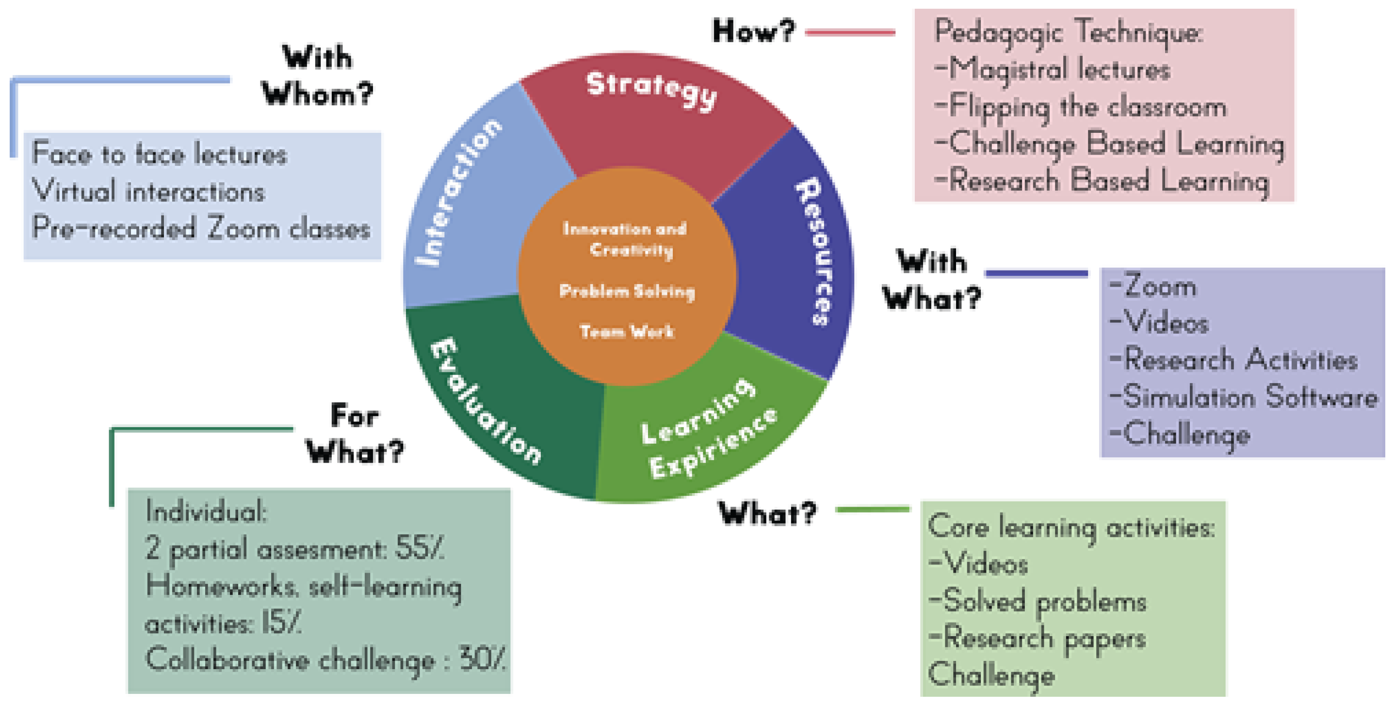
2. Method-DidacticProposal for an Active-Collaborative Learning Massive Flexible Digital Master Class

The didactic proposal has the following elements: an overview of the educational research methodology, the disciplinary and transversal competencies, and the proposal’s design around the teaching–learning process.

2.1. Educational Research Methodology

The work presented herein is part of an educational research study, where the goal is to study the effect of a phenomenon in the context of active learning. It is a mixed-method approach that will include quantitative (numerical information from closed-form questions in an anonymous a posteriori student questionnaire) and qualitative (teachers’ field notes and students’ open-form questions of the previously mentioned student questionnaire) information during the activity´s implementation. The methodology is based on educational inquiry approaches, reported, analyzed, and explained by experts in the area [42,43,44].

2.2. Disciplinary and Transversal Competencies

Without being limited to a specific text of competencies defined for a unique undergraduate academic program in engineering, this proposal is intended to develop the following sub-competencies in students:
  • The student obtains a mathematical model of the dynamics of a direct current motor (disciplinary).
  • The student validates the mathematical model through simulation work (disciplinary).
  • The student works collaboratively to develop effective communication and reasoning for complexity (transversal).
The previous competencies are planned to be developed by students enrolled in any of these undergraduate engineering programs: electrical, electronic, and mechatronic. The specific courses of the curriculum would be electrical systems, electrical actuators, or automatic control systems.

2.3. Didactic Techniques—Collaborative Learning and Flipped Classroom

The chosen didactic techniques enable the adequate deployment of the activity and enable application of the proposed methodology. Collaborative learning is oriented to work in small groups, which in this case are of two people, where the participants share their work and discuss what each one developed, in order to later cooperate in the following stages. Additionally, the flipped classroom enables—through asynchronous work—students to advance in the activity and optimize the time of the synchronous sessions. This combination of techniques enables students to advance over time and to develop the declared sub-competencies for the activity.

2.4. Proposal—Didactic Design

The work to be carried out consists of several stages that stimulate students to build their learning and enrich it more and more as they progress through the activities. The proposal considers teams of two people and it comprises a review of the modeling theory of direct current (DC) motors to the simulation of an automatic control loop that uses the previously developed and validated mathematical model. There are three synchronous sessions (teacher and all students) and three asynchronous periods (working in teams of two people).
The flipped classroom is observed in the learning activities carried out outside the synchronous sessions. These activities imply responsibilities of each team member that must be fulfilled in a certain time and whose results will be used in the synchronous sessions. Failure to perform them properly would imply a considerable delay in the advance of synchronous work or even not being able to continue advancing on the global activity.
Collaborative learning lies in the design of the activity that demands an integration of the findings and results of each member to continue advancing with the global activity. There are five time frames where collaboration is the only way to reach the next result. In this scheme, the teacher becomes a mentor and guide instead of a provider of knowledge.
The motivation will be generated by collaborative work inside and outside the classroom (flipped classroom), and it is expected to develop a sense of team achievement, because results are obtained together, which opens the door to more advanced phases of the activity. Moreover, these didactic techniques are expected to help develop decision-making skills, effective communication, and reasoning for complexity while the students solve the stages of global activity and also develop disciplinary competencies.

2.5. Breakdown of Activities

The activity will take place in teams of two people who will work collaboratively in stages. Students will work in an individual and collaborative format to obtain knowledge and develop competencies. During the deployment, they will be accompanied by the teacher to take care of the correct progress and fulfillment of each stage, and to resolve doubts during the activities.
The complete set of activities has been designed to be carried out in a three-session format; each one with previous outside-the-classroom work and in-class tasks.
  • Session 1—Previous:
    I
    All participants review the description, competencies, expected outcomes, schedule, milestones, and policies related to the activity. The professor introduces the topic and remarks on the importance of dynamic models and automatic control in engineering. Herein, the competencies are illustrated, and the expected results and breakdown schedule is presented to the students.
    II
    Students (in teams) review the theory about mathematical modeling of DC motors in the textbook or in any other designated media.
    III
    Separately, each student develops the mathematical model, and later on, they incorporate both efforts into one single model that is the deliverable of the previous activity. They will also carry out a qualitative validation of the obtained model before moving on to the next stage. It is likely that one or both students will have to carry out this stage again if there are problems with the expected model behavior.
    IV
    Students review podcasts with introductory tutorials about Scilab.
  • Session 1—During:
    I
    The professor summarizes the activity description and all related information.
    II
    The teacher presents the mathematical model, discusses results, and resolves doubts about the procedure.
    III
    In a plenary session, the obtaining of the block diagram that models the engine is presented and worked on, and the input and output relationships of interest are clarified.
    IV
    Each team builds the block diagram in Scilab. They will adjust parameters and review input–output relations.
    V
    The teams program the differential equations that represent the system and review the input–output relations.
    VI
    In a plenary activity, students compare differential equations versus the block diagram representations.
  • Session 2—Previous:
    I
    Students review material to become familiar with it (Quite Universal Circuit Simulator), and solve introductory exercises.
    II
    (in teams) In Qucs, student A programs the electrical circuit that models the motor’s dynamics.
    III
    (in teams) In Scilab, student B validates the result in Qucs by programming a numerical analysis.
    IV
    Each student will explain to their partner what they did. The level of mastery must be such that each member must be able to understand and modify the partner’s work.
  • Session 2—During:
    I
    Each member will work with the results of the other associate towards carrying out the following tests: no-load test with a constant supply voltage, no-load test with a pulse width modulation (PWM) supply voltage, and load test with a constant supply voltage.
    II
    The team share experience and results, and record observed similarities and differences.
    III
    The main findings are highlighted in a plenary activity.
    IV
    The professor will introduce control systems stability, Lyapunov stability analysis, and PID (proportional–integral–derivative) controllers.
  • Session 3—Previous:
    I
    Students will reinforce the previously explained control-oriented topics through defined material (videos and preliminary examples).
    II
    The teams will start to develop the mathematical procedure to test stability in closed-loop with a PD controller, and the achievements will be delivered.
  • Session 3—During:
    I
    In a plenary session, the professor will carry out the mathematical stability procedure and resolve queries.
    II
    Teamwork to simulate the closed-loop in Scilab will be accomplished.
    III
    Main results and conclusions are discussed among all participants.
    IV
    All activities are delivered in a single report (one per team).

2.6. Outcomes and Evidence

Each activity outside and inside the synchronous sessions generates a partial deliverable (written report, log file, and simulation files) that will integrate the final report. This document includes theoretical aspects, carried out activities (including simulation work), findings, problems and their solutions, and learning achieved during the activity.
Additionally, each team will record a video (collaboratively participation) where they will summarize the most important points of the activities. The evidence of the development of competencies will be comprised of the final report, the simulation work, and the video. The evaluation rubric will consider students’ participation during all the sessions, the evidence, and all the results. To motivate collaborative work and learning, team-generated findings and results are also included as part of the evidence.

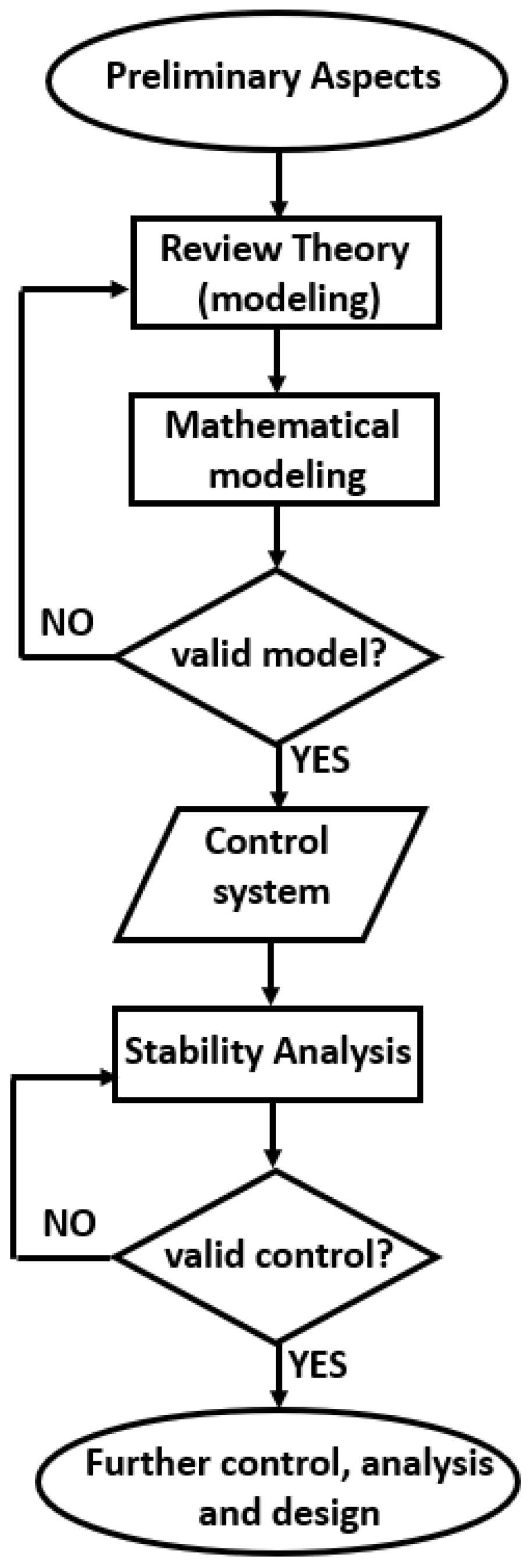
2.7. Competency-Oriented Flowchart

The flow diagram of the didactic proposal stages, that will be developed by the students, is presented in Figure 1. The flowchart considers possible rework due to opportunity areas detected during the modeling or control phases.

2.8. Activity Deployment

The implementation of this proposal in a Massive Flexible Digital Masterclass (MFDM) environment requires certain conditions. The activity is for sophomore engineering students who have already taken the following courses: electricity and magnetism, electrical circuits, differential equations, programming, and control engineering. The case study is planned for credit compulsory/elective courses. The semester and the name of the course have not been defined, as it will be applied to different engineering academic programs with their specific courses.
An MFDM environment allows following more than 100 students if they have access to the required software and the teacher is given time to follow up on the students. For the implementation, a group size between 100 and 120 students is proposed, which is an acceptable quantity in traditional mass classes. In addition to internet access, the necessary technological resources are the digital platform for the teacher to carry out the MFDM and communicate with the students and a computer with simulation software for each student. Moreover, students would make the teams on their own. Sophomore students have teamed up with some colleagues and the suggested approach is that they form teams with whom they are better connected to collaborate. More information about an MFDM is available in Appendix A.

3. The Case Study: Modeling, Simulation, and Control of a DC Motor

This section is focused to explain in detail the mathematical and simulation work that students will develop, as well as the expected results for each phase of the activity.

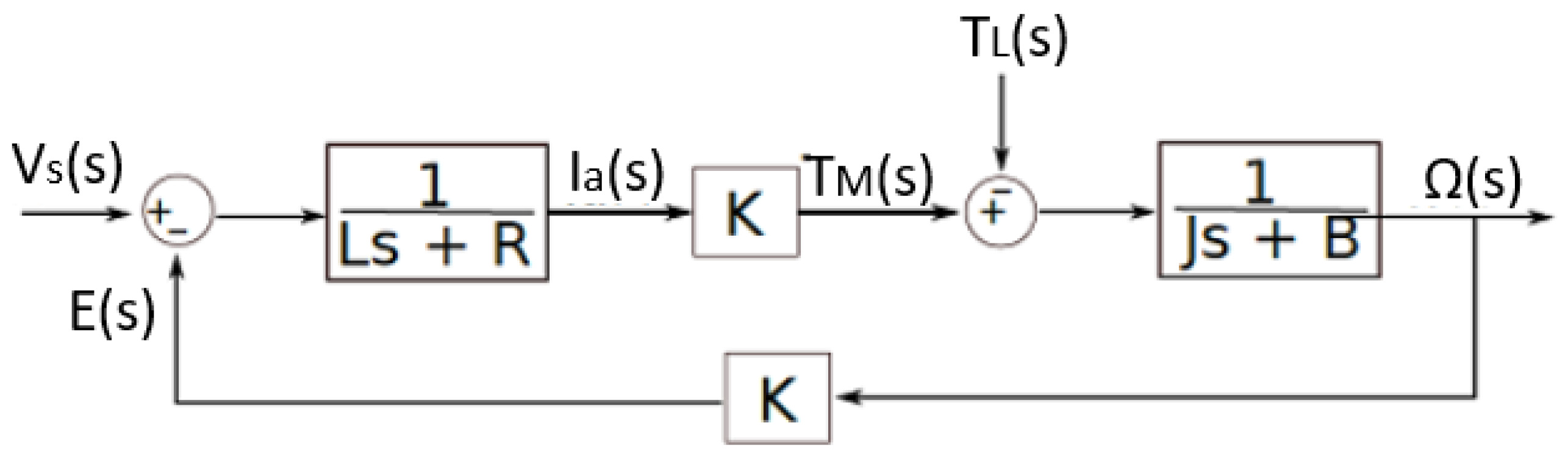
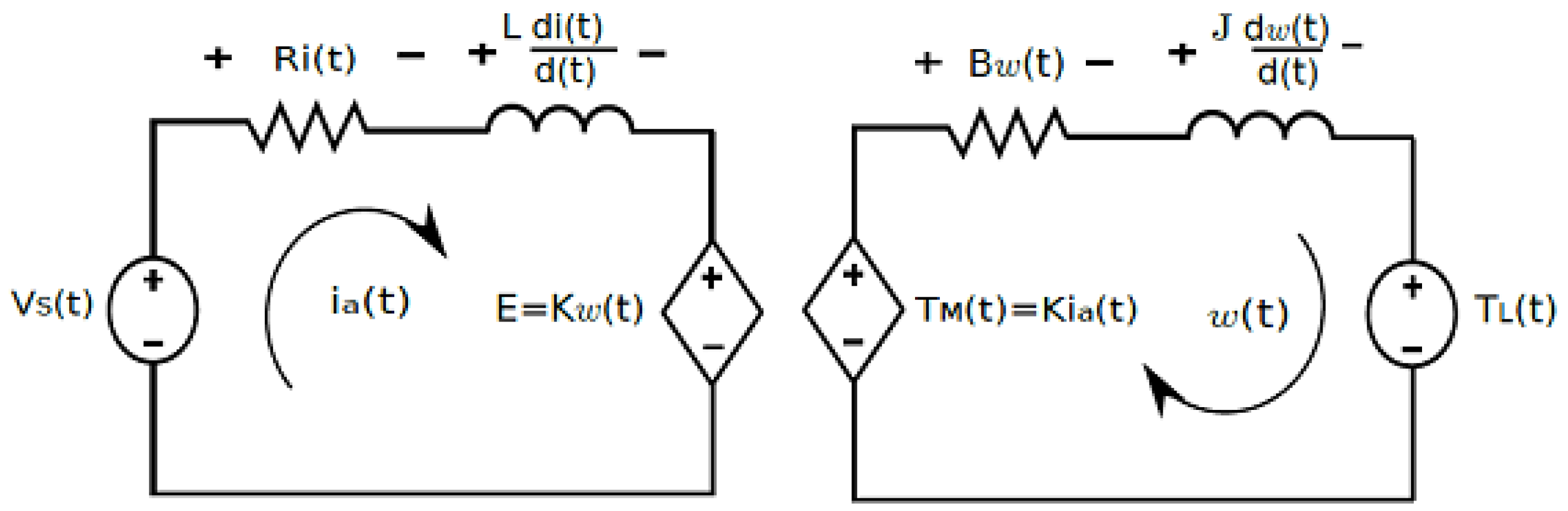
3.1. Mathematical Modeling—Understanding the System’s Dynamics

The electrical circuit of a DC motor comprises the supply voltage, v s ( t ) , the armature resistance, R, the armature’s inductance, L, and the induced voltage, e ( t ) , as shown in Figure 2. As similarly stated in [22,23,24,30,45], Equation (1) can be written by using Kirchhoff’s law, where i a ( t ) is the armature current and t represents the time.
v s ( t ) + R i a ( t ) + L d i a ( t ) d t + e ( t ) = 0
As described in [16], the induced voltage, e ( t ) , can be substituted by an electrical constant, K E , and an angular velocity, ω ( t ) , as can be identified in Equation (2).
e ( t ) = K E w ( t )
As similarly specified in [19,22,24,27,29,30,45], and according to Newton’s second law in its angular form, Equation (3) can be defined.
T M ( t ) B ω ( t ) T L ( t ) = J α ( t )
In Equation (3), T M ( t ) represents the total electromechanical torque developed by the motor’s shaft, J is the inertia moment constant, B is the friction constant, T L ( t ) is the load torque, and α ( t ) is the angular acceleration. Rearranging terms, and recalling that α ( t ) is also the variation of the angular velocity regarding time, Equation (4) shows how the motor’s torque, T M ( t ) , has to overcome the torque losses caused by the inertia, friction, and load torques.
T M ( t ) = B w ( t ) + J d w ( t ) d t + T L ( t )
As indicated in [16], the electromagnetic torque, T M ( t ) , in Equation (4), is equal to the mechanical constant, K M , multiplied by the armature current, i a ( t ) , as can be seen in Equation (5).
T M ( t ) = K M i a ( t )
For practical purposes, it is assumed that the electrical constant, K E , and the mechanical constant, K M , are equal, as shown by Equation (6); hence, from now on, both constants are going to be represented with K. The equivalence of both constants is demonstrated in [16], where the dimensional analysis between the units of Vs and Nm/A, as well as their relation with the physical unit W e b e r , is remarked, as shown in Equation (7).
K = K M = K E
K E V s W b = K M N m A W b
If the system is modeled with a permanent magnet motor, or the field current is constant, then the system of differential equations that model the DC motor is given by Equations (8) and (9), where the supply voltage has to provide the necessary electromotive force for all the voltage drops. In addition, it can be noticed that the electromagnetic torque, T M ( t ) , in Equation (4), has been substituted using Equations (5) and (6).
v s ( t ) = R i a ( t ) + L d i a ( t ) d t + K w ( t )
K i a ( t ) = B w ( t ) + J d w ( t ) d t + T L ( t )
Figure 2 shows a block diagram of the DC motor model in the S-domain, where it is possible to notice that the torque T M ( s ) is proportional (K) to the current I a ( s ) . Furthermore, the minus sign and the gain K in the feedback path represent a shaft speed, Ω ( s ) , that is opposite to the supply voltage, V s ( s ) , by means of the induced voltage, E ( s ) , i.e., E ( s ) = K Ω ( s ) .

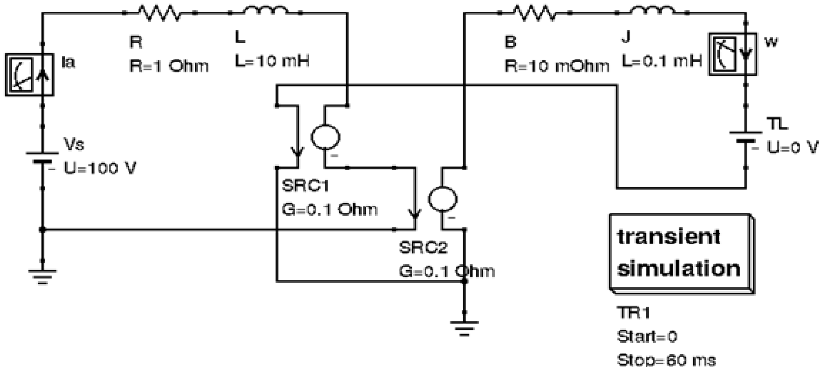
3.2. Circuit Simulation in Qucs—A Purely Electrical System

Figure 2 in the S-domain can be re-drawn in the time domain by using the circuit schematic, as shown in Figure 3. It consists of two closed loops where the left path is mostly electrical except for the induced voltage, e ( t ) , which depends on the angular velocity, ω ( t ) , of the rotor. The right path is mostly mechanical except for the electromagnetic torque, T M ( t ) , which depends on the armature current, i a ( t ) .
In Figure 3, both paths depend on each other when i a ( t ) and ω ( t ) have to be solved simultaneously. As shown in Figure 2, the constant K transforms the armature current, I a ( s ) , into the developed torque, T M ( s ) . Because the constant K is the only parameter involved in the electromechanical conversion, the inverse transformation from the S-domain into the time domain is direct. Assuming that there is a current flowing through the path of the right side with the same magnitude and units matching those of the angular velocity, ω ( t ) , and letting the mechanical torques T M ( t ) , B ω ( t ) , J ω ( t ) , and T L ( t ) , to be seen as voltage supplies and drops, then, by Kirchhoff’s law, Equation (9) can be analyzed from another perspective.
The circuit in Figure 3 can be simulated to study its behavior. The effort proposes Qucs (Quite Universal Circuit Simulator), which is a free software circuit simulator released under general public license (GPL) [46]. As shown in Figure 4, probes were added to measure i a ( t ) and ω ( t ) . For simulation work, the applied motor’s parameters are listed in Table 2.
Besides the numerical values in Table 2, the following parameters contributed to stimulate the system sufficiently and to visualize transient and steady-state responses suitable for the purposes of the activity. A constant supply voltage v s = 100 V has been defined as the system’s input, and a no-load torque has been added, i.e., T L ( t ) = 0 Nm. The transient simulation option has been selected along with a simulation time of 60 ms and a sampling period of 10 ms, and 6001 samples have been used to collect the data. Furthermore, the initial currents across the inductors had no default values, and they have been manually chosen to be zero, i.e, the armature was not initially energized while the rotor was at rest. Figure 3 shows that the current-dependent voltage sources take the current from their counterpart circuit and that the conversion factor of these dependent sources has to match the electromechanical constant K, which has units of Webers.

3.3. Numerical Simulation—A Validation in Scilab

To validate the results obtained from the electric circuit analogy, a numerical analysis was performed by using the Euler method of the form y ( n + 1 ) = h f ( y n , t n ) + y n , to solve the system of differential equations, where h is the simulation step time as explained in [47,48]. To accomplish this task, a free licensed numerical software package called Scilab was employed [49]. By assuming a small increment in time equal to the sampling period, i.e., h = Δ t , Equations (8) and (9), were discretized to generate Equations (10) and (11), where i ( t = 0 ) = 0 and ω ( t = 0 ) = 0 were defined as the initial conditions—i.e., at t = 0 s there was neither armature current nor rotor speed.
v s ( t ) = R i a ( t ) + L i a ( t + Δ t ) i a ( t ) h + K w ( t )
K i a ( t ) = B w ( t ) + J w ( t + Δ t ) w ( t ) h + T L ( t )
With the n index for simulation purposes where h = Δ t , Equations (10) and (11) were programmed as in Equations (12) and (13), where the first simulation values matched the initial conditions—i.e., i a ( n ) = 0 and ω ( n ) = 0 when n = 1 .
i a ( n ) = h L V s ( n 1 ) R i a ( n 1 ) K ω ( n 1 ) + i a ( n 1 )
ω ( n ) = h J K i a ( n 1 ) B ω ( n 1 ) T L ( n 1 ) + ω ( n 1 )

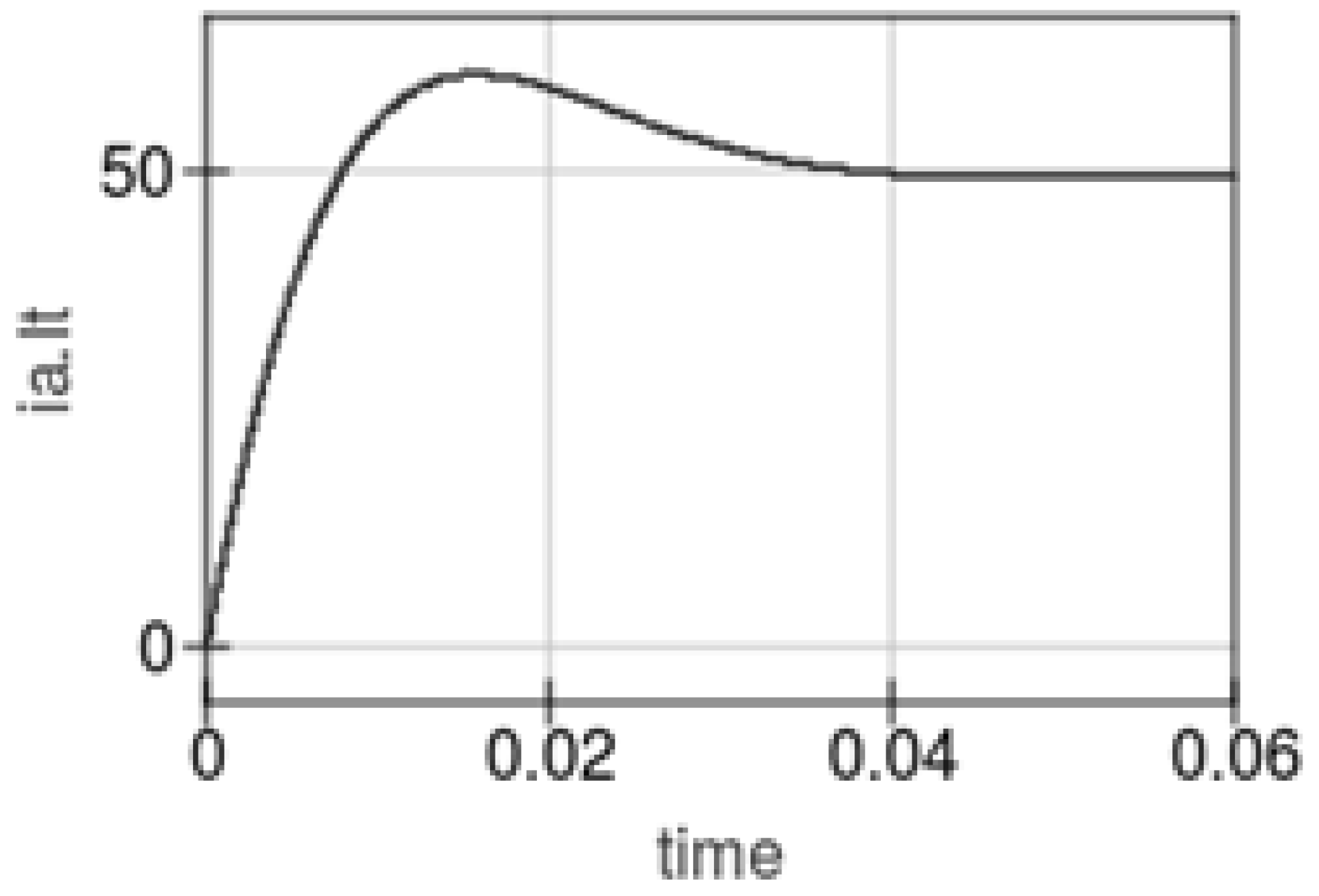
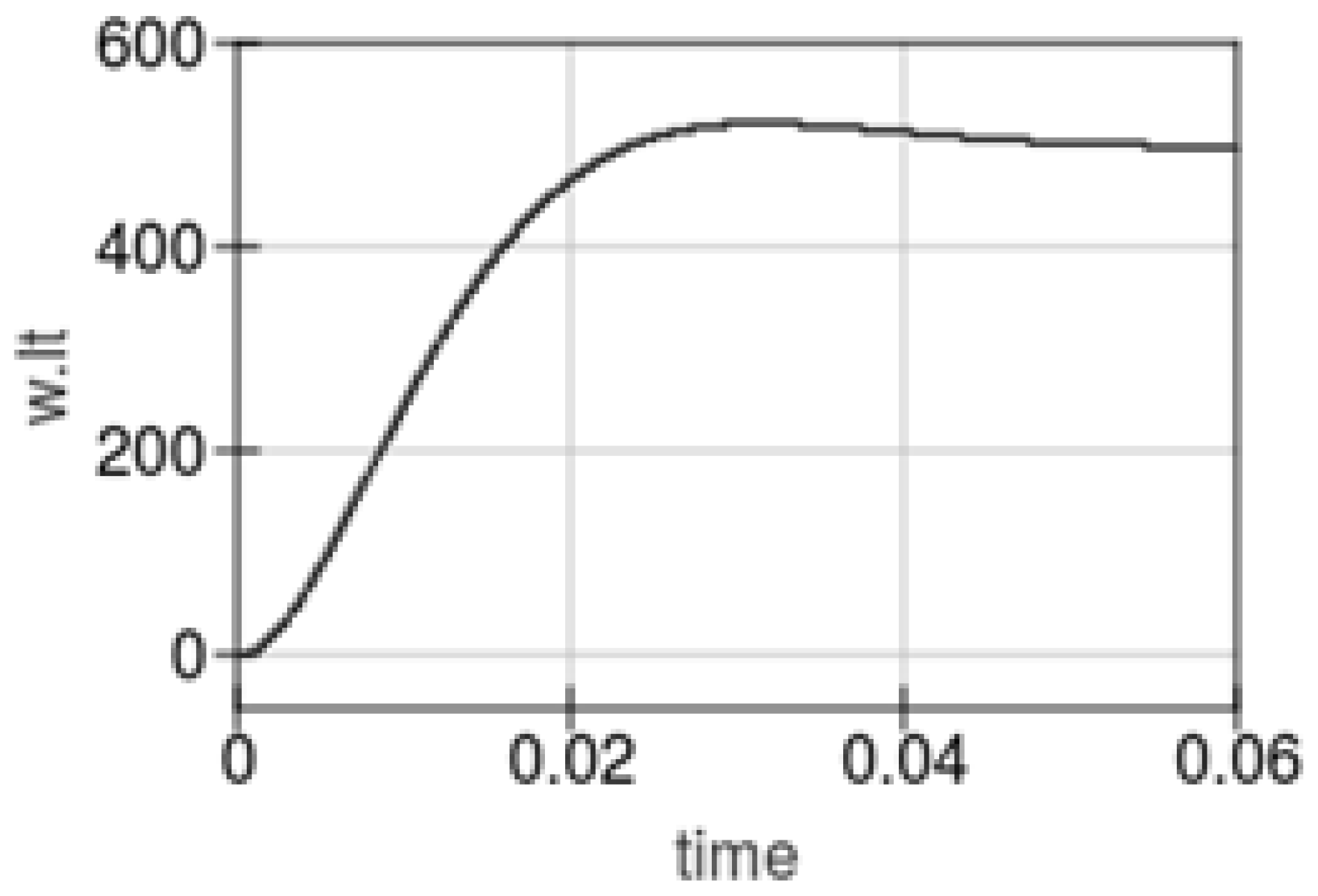
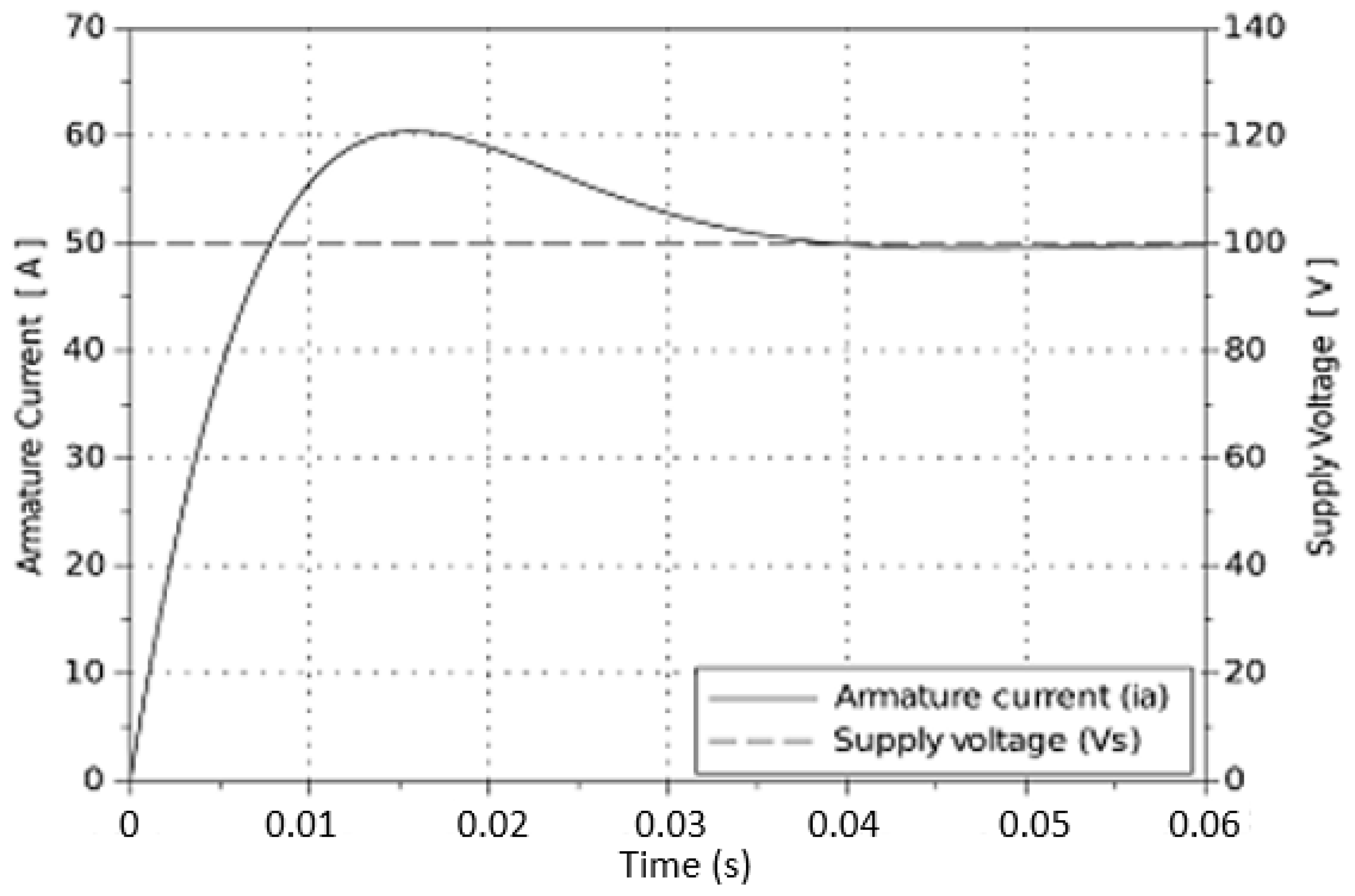
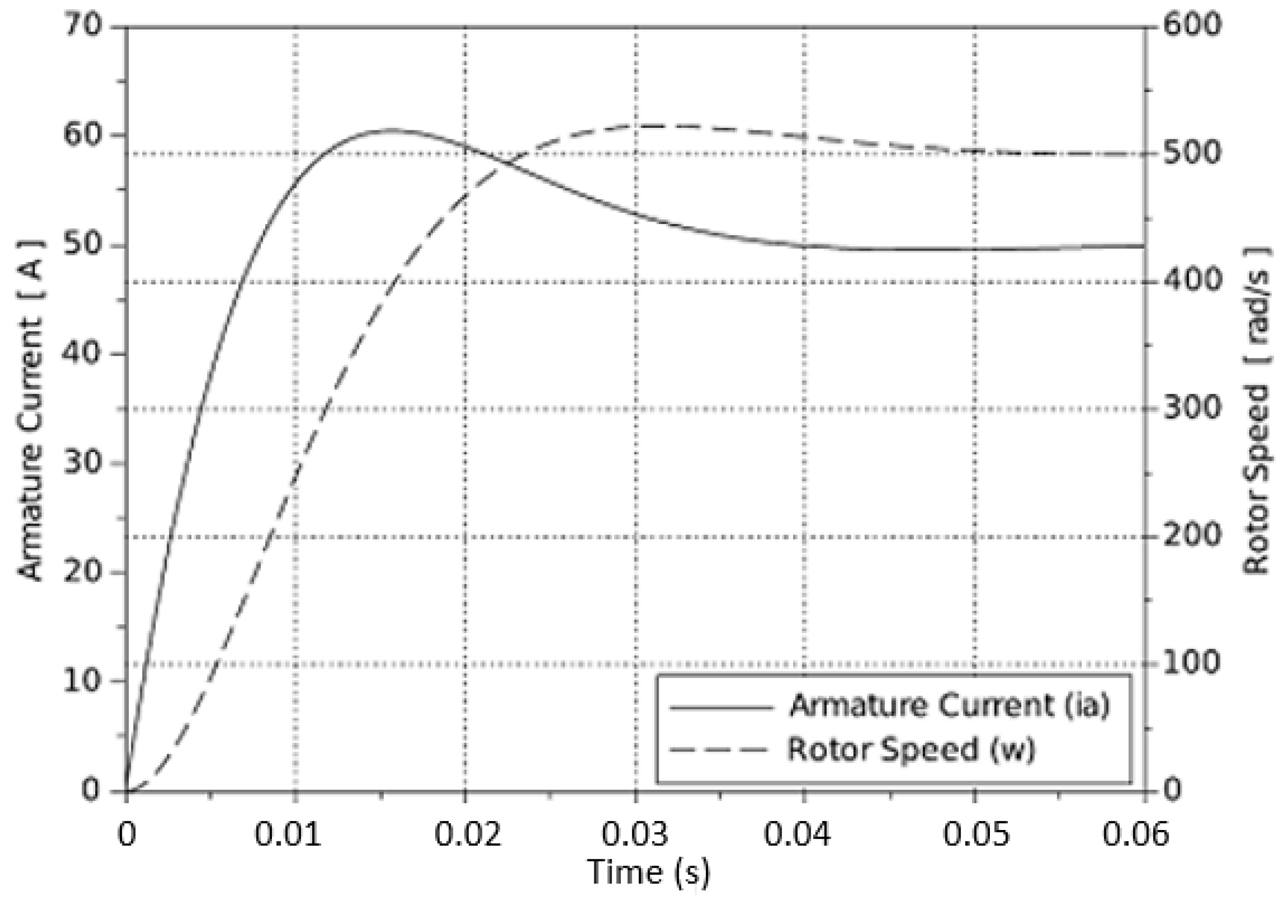
3.4. Results in the Open-Loop

The following subsections explain the different open-loop testing scenarios in Qucs and Scilab, the findings, and the comparison of results contained between the simulators.

3.4.1. No-Load Test with a Constant Supply Voltage

Using Qucs simulator, the behavior of the armature current, when using a constant supply voltage of v s = 100 V and a zero-load torque T L = 0 Nm, is shown in Figure 5, where the y-axis measures the no-load tests i a ( t ) in Amperes, and the x-axis represents the time in seconds. Figure 6 shows the angular speed of the rotor under the same conditions, and the y-axis refers to ω ( t ) in radians per second.
With the programming-oriented Equations (12) and (13), Figure 7 and Figure 8 were generated in Scilab. These two graphs obtained in Scilab are similar to those generated in Qucs. Figure 7 shows the armature current, i a ( t ) , and the supply voltage, v s ( t ) . Similarly, Figure 8 shows the armature current, i a ( t ) , and the rotor speed, ω ( t ) . For the Scilab simulation work, these parameters were defined to graph the transient and steady-state response: a simulation time equal to 60 ms, a sampling period of 10 ms, and 6001 samples.

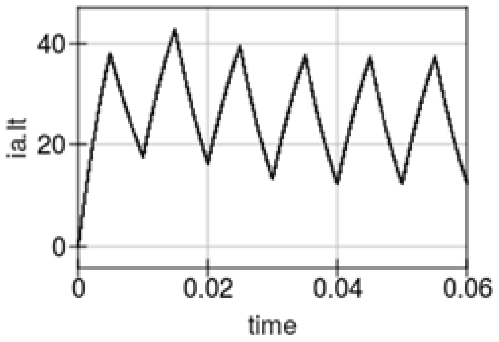
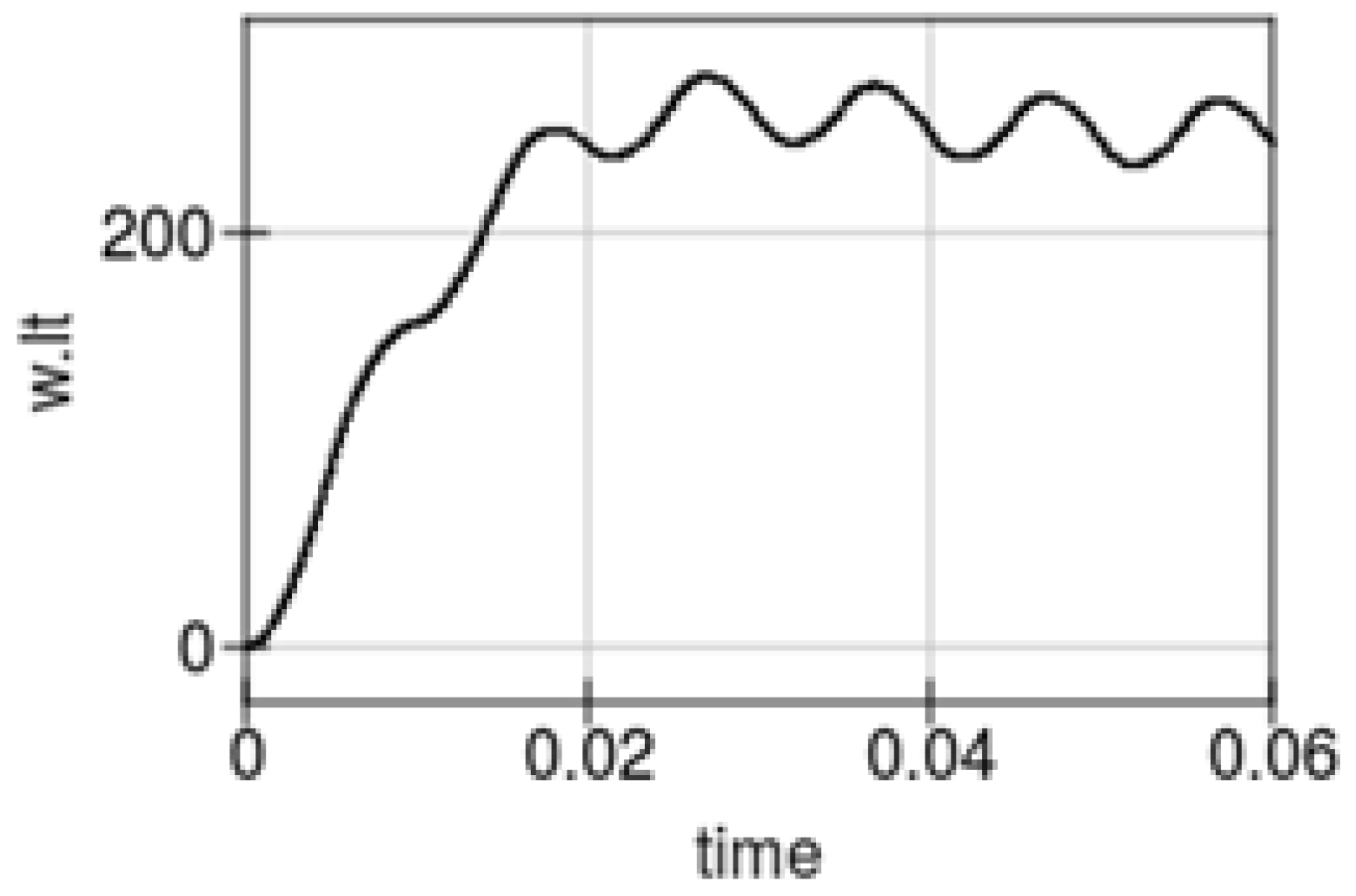
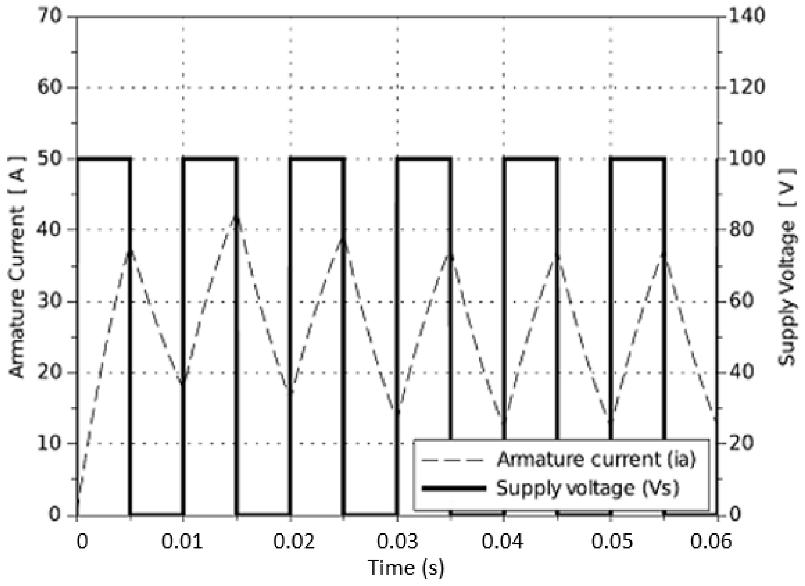
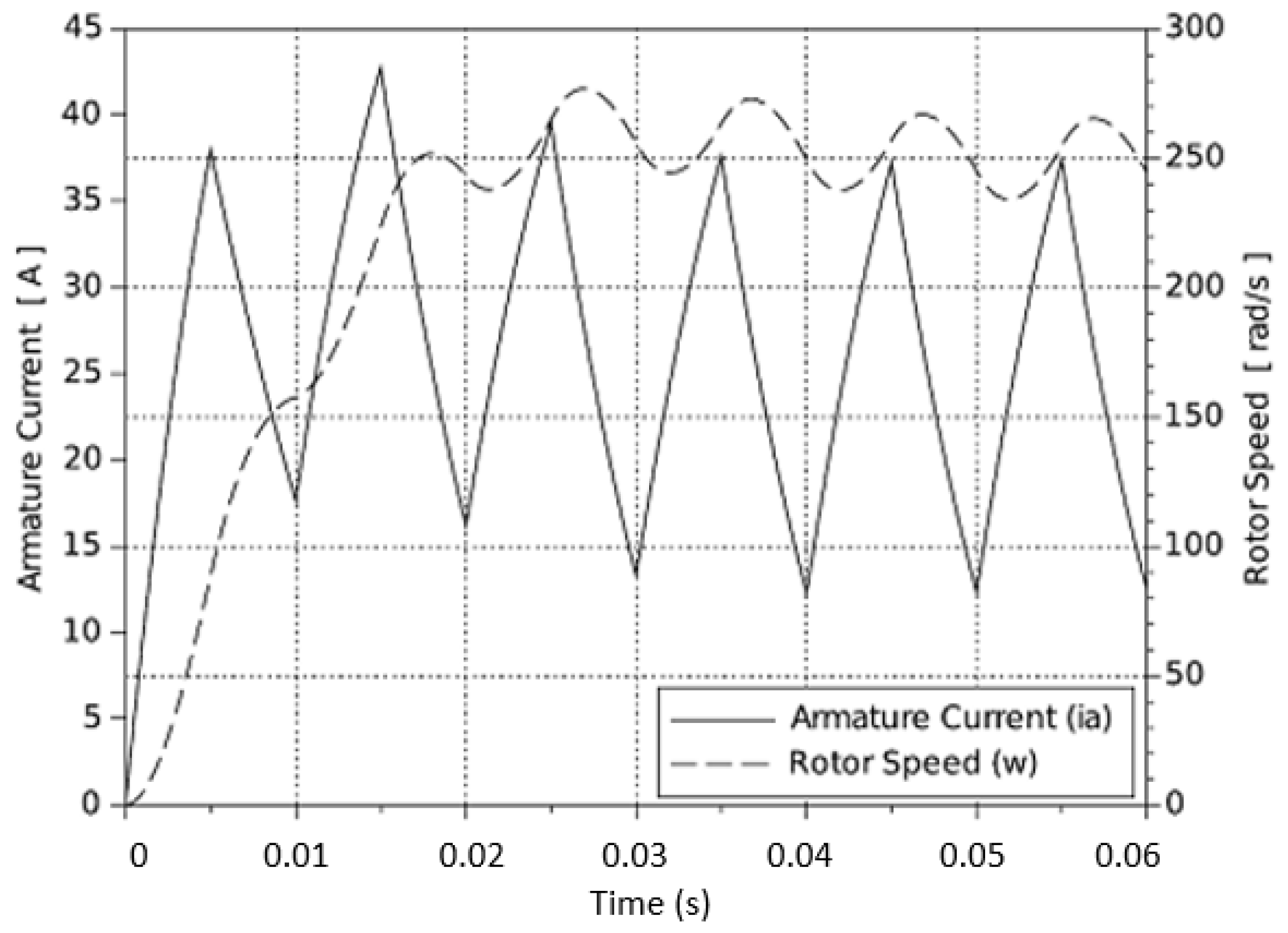
3.4.2. No-Load Test with a Pulse-Width-Modulated (PWM) Supply Voltage

In this subsection, the electric circuit analogy is tested by using a pulse width modulation (PWM) supply voltage with a peak value of 100 V, a duty cycle of 50 % , and no-load conditions. The results are plotted and qualitatively compared against the solutions provided by solving the system of differential equations in Scilab. The simulation parameters are similar to those employed for the no-load test—i.e., a simulation time of 60 ms, a sampling period equal to 10 ms, and 6001 samples—to generate the graph. It is important to mention that, to simulate the PWM voltage using Qucs, a rectangle input voltage signal was selected with rising time t r = 0 s and falling time t f = 0 s. Figure 9 and Figure 10 portray, in Qucs, the armature current, i a ( t ) , and the angular velocity, ω ( t ) , respectively.
The next step was to obtain the same variables i a ( t ) and ω ( t ) with the free licensed software, Scilab, to validate the results by running a qualitative comparison with the results in Qucs. Figure 11 and Figure 12 illustrate the simulation outcomes in Scilab.
By comparing the behavior of i a ( t ) in Figure 9 versus Figure 11, and ω ( t ) in Figure 10 versus Figure 12, it can be seen that the solutions of the circuit analogy simulated in Qucs agree with the results provided by Scilab.

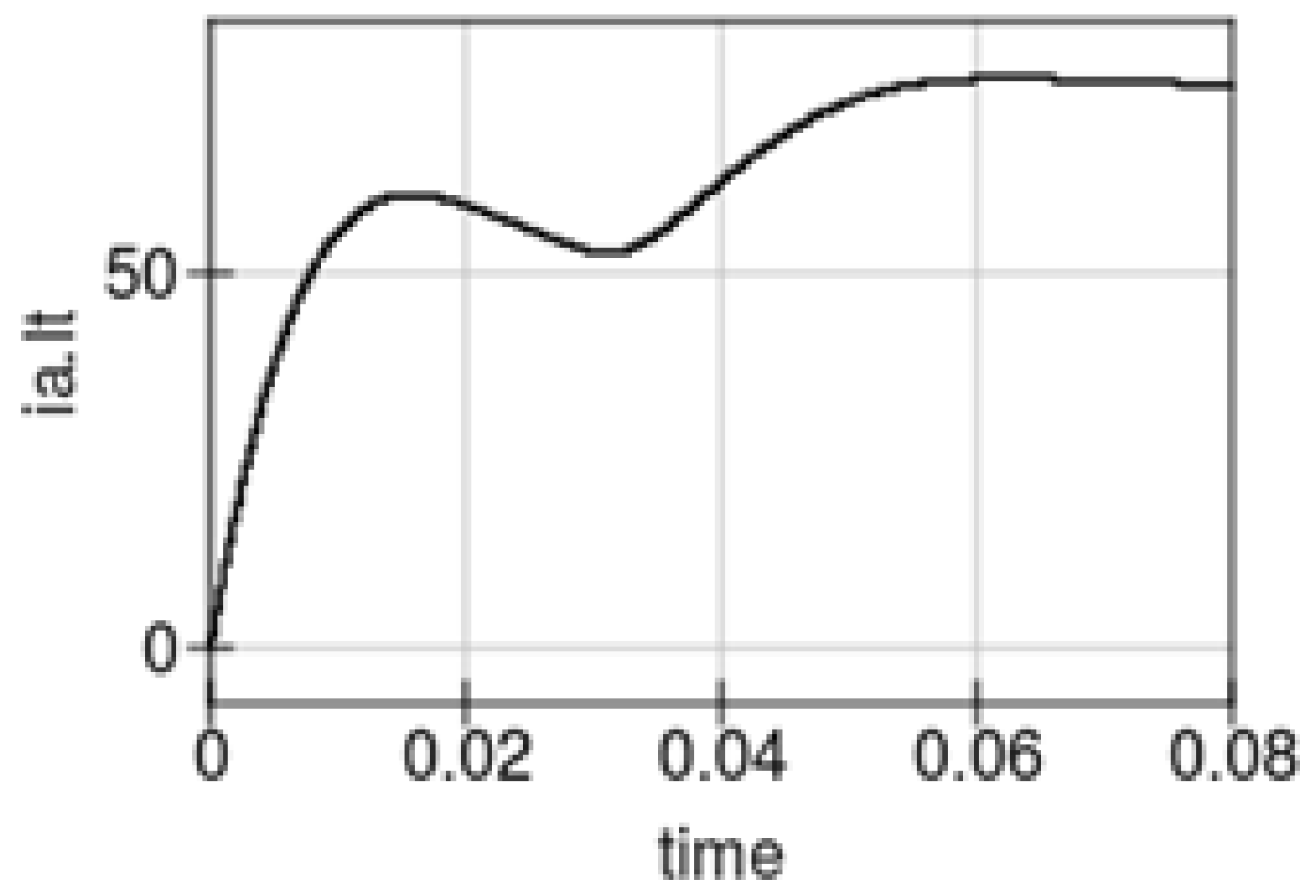
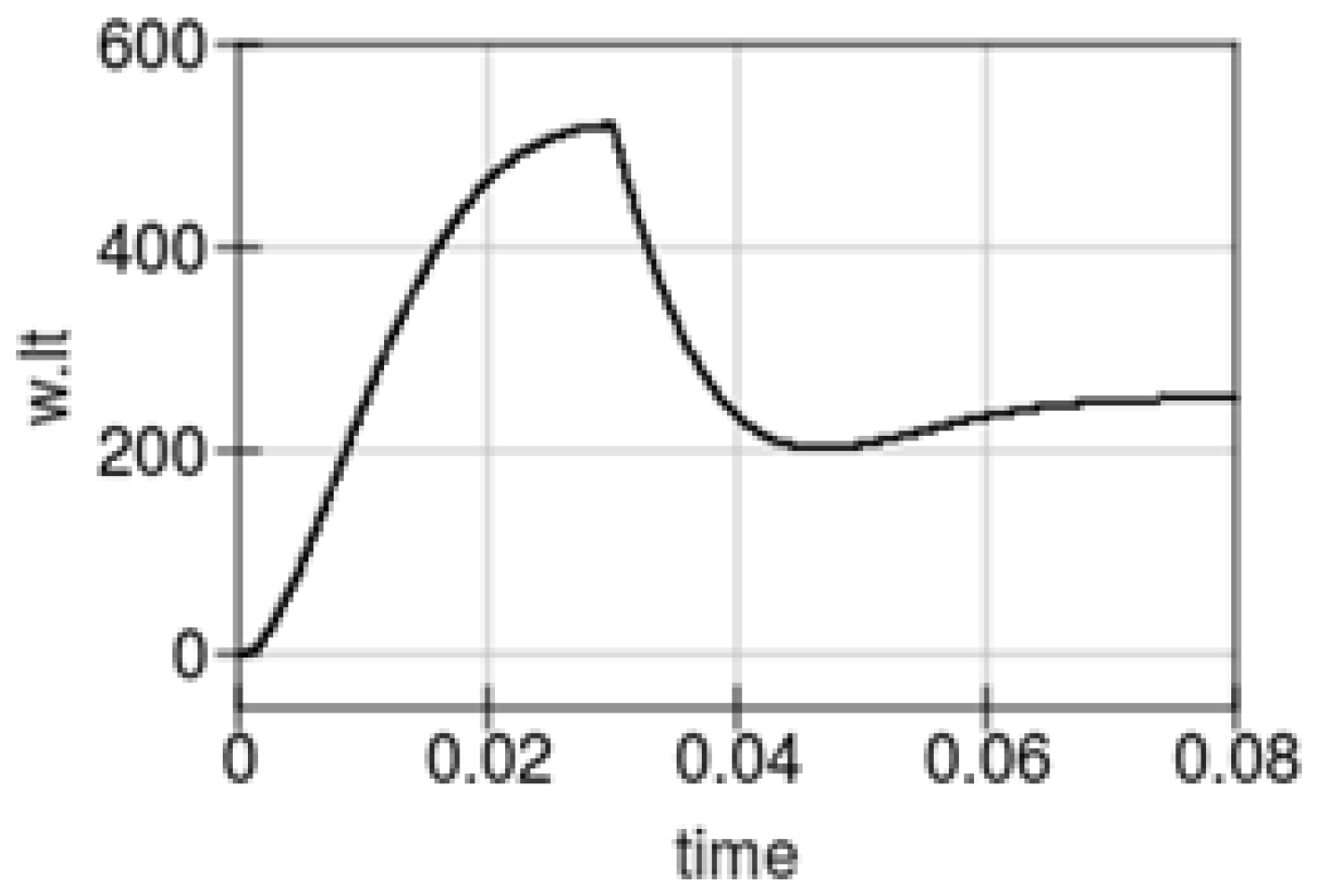
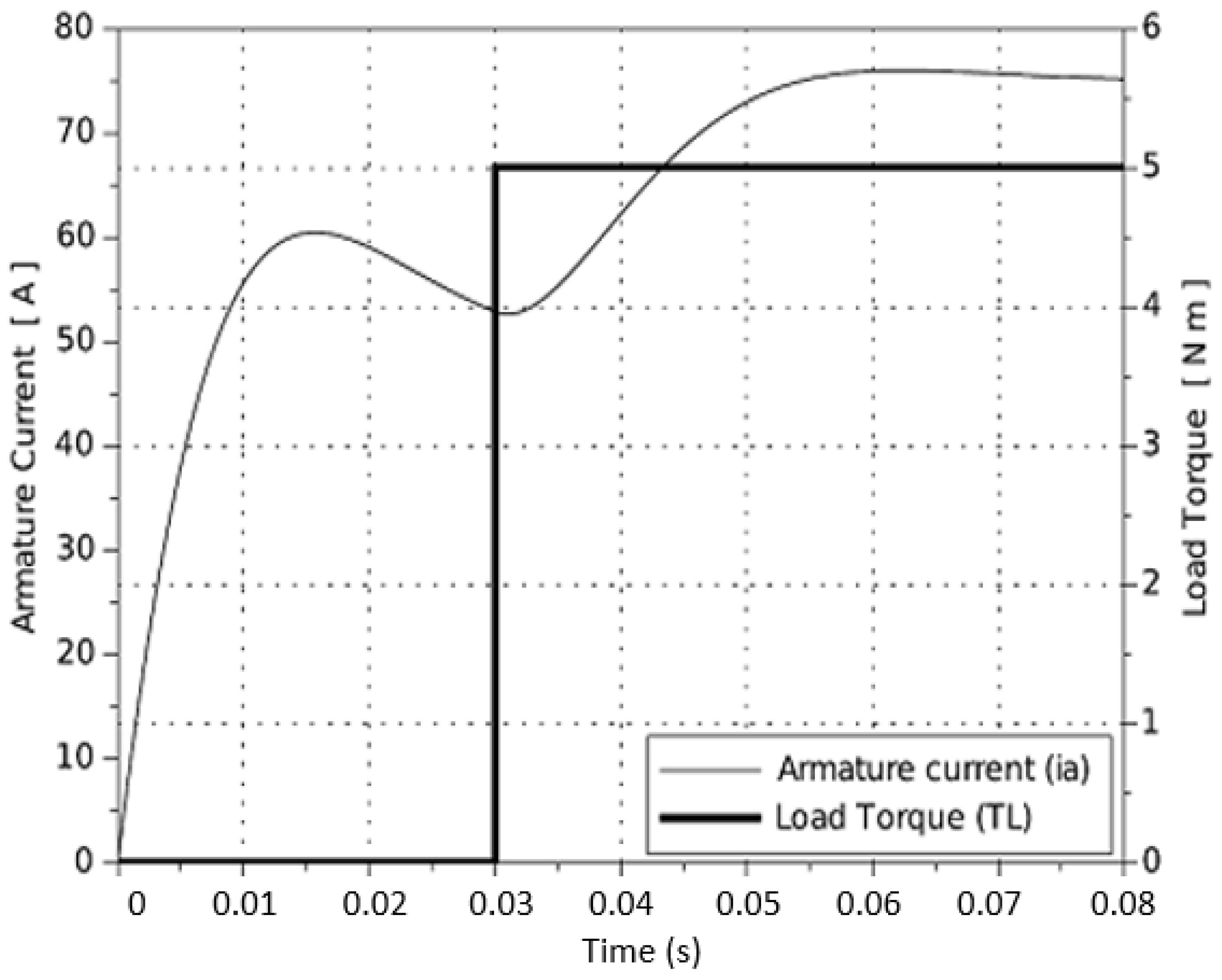
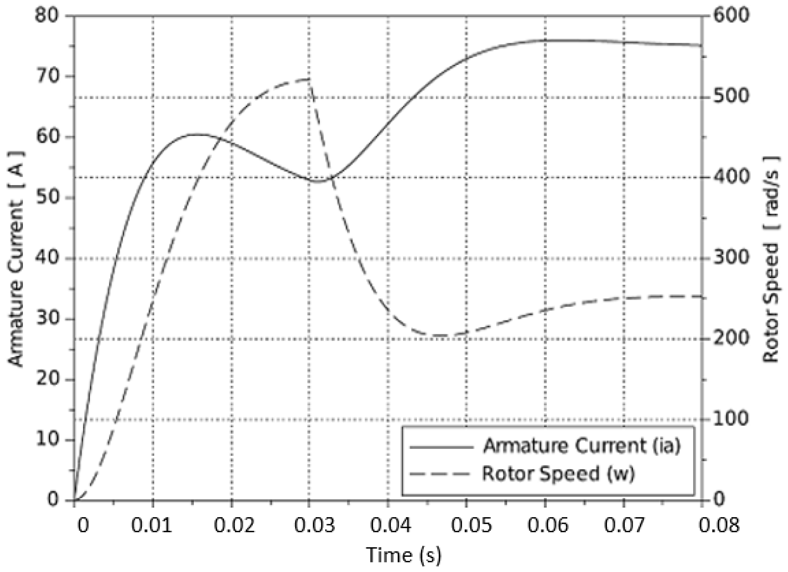
3.4.3. Load Test with a Constant Supply Voltage

It is also important to test the DC motor performance under load conditions. For the same outcomes in Equations (12) and (13), responses for i a ( t ) and ω ( t ) were obtained in Qucs, and the results are depicted in Figure 13 and Figure 14, respectively. The simulation parameters are constant supply voltage v s ( t ) = 100 V, a load torque equal to 5 Nm (implemented in Qucs, a voltage pulse component with an amplitude of 5 V, a start time of 0.03 s, and a stop time of 0.08 s have been selected). Additionally, the sampling period was 10 ms, and 8001 samples were collected to generate the graph.
To analyze in Scilab, the behavior of the armature current and the rotor’s angular velocity—depicted in Figure 13 and Figure 14, as well as Equations (12) and (13)—were applied for the load test with a load torque equal to 5 Nm. Responses for i a ( t ) and ω ( t ) in Scilab are shown in Figure 15 and Figure 16, respectively.

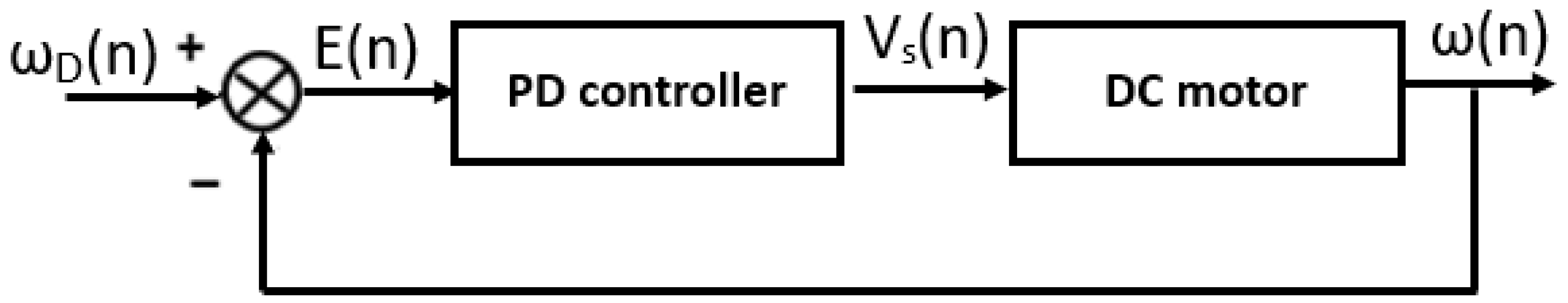
3.5. Discrete PD Control and Stability Analysis

The following subsections develop the stability analysis in closed-loop, considering a negative and unitary gain feedback loop with a proportional–derivative controller.

3.5.1. Discrete-Time PD Controller

In the context of a motor model defined for numerical integration with iterative equations, based on an index n, the control work was carried out in the discrete-time domain. The discrete-time version of the continuous-time PD controller, through the Euler’s approximation, can be written as follows:
R i a ( t ) + L i a ( t + Δ t ) i a ( t ) Δ t + K w ( t ) = K p e ( t ) + K D e ( t + Δ t ) e ( t ) Δ t
If ω D ( t ) is defined as the desired angular velocity, and ω ( t ) stands for the controlled variable, and if the proposed closed-loop system has a negative and unitary feedback signal, then the error is defined as e ( t ) = ω D ( t ) ω ( t ) ; then, Equation (14) can be rewritten as Equation (15).
R i a ( t ) + L i a ( t + Δ t ) i a ( t ) Δ t + K w ( t ) = K p ω D ( t ) ω ( t ) + K D d e ( t ) d t
which can be rewritten as follows:
R i a ( t ) + L i a ( t + Δ t ) i a ( t ) Δ t + K w ( t ) = K p ω D ( t ) ω ( t ) + K D ω D ( t + Δ t ) ω ( t + Δ t ) ω D ( t ) ω ( t ) Δ t
In practice, it is hard to know the future values of the desired angular velocity; thus, constant values for this variable were selected for simulation purposes, as defined in Equation (17).
ω D ( t + Δ t ) = ω D ( t ) = ω D
Using Equations (8) and (17), the discrete control law for the voltage v s ( t ) , that is applied to the motor, is defined in Equation (18), where the variable n is the discrete index.
V s ( n ) = K P ω D ω ( n ) + K D Δ t ω ( n ) ω ( n + 1 )
The waveform of ω ( t ) and i a ( t ) can be calculated in discrete-time domain by Equations (19) and (20).
ω ( n ) = Δ t J K i a ( n 1 ) B ω ( n 1 ) T L ( n 1 ) + ω ( n 1 )
i a ( n ) = Δ t L K P ω D ω ( n 1 ) K ω ( n 1 ) R i a ( n 1 ) + K D L ω ( n 1 ) ω ( n ) + i a ( n 1 )

3.5.2. Stability Analysis

This subsection develops a stability analysis of the DC motor based on Lyapunov stability theory. The study starts with the discrete-time version of the system’s state–space representation.
x 1 ( n + 1 ) = R L x 1 ( n ) K L x 2 ( n ) + 1 L u ( n )
x 2 ( n + 1 ) = K J x 1 ( n ) B J x 2 ( n ) + 1 J u ( n )
The proposed discrete-time Lyapunov stability condition is:
Δ V ( x 1 , x 2 ) = V f ( x 1 , x 2 ) V ( x 1 , x 2 )
and the proposed Lyapunov candidate function is:
V ( x 1 , x 2 ) = 1 2 ( x 1 2 + x 2 2 )
With the insertion of Equation (23) into the Lyapunov candidate function in Equation (24), and with a mathematical simplification, Equation (25) is obtained.
Δ V ( x 1 , x 2 ) = 1 2 ( R 2 L 2 + K 2 J 2 1 ) x 1 2 + ( R 2 L 2 + B 2 J 2 1 ) x 2 2 + ( 2 R K L 2 K B J 2 ) x 1 x 2
To achieve asymptotic stability, it is necessary that Δ V ( x 1 , x 2 ) 0 . To guarantee this, the following conditions must hold:
R 2 L 2 + K 2 J 2 1 0
R 2 L 2 + B 2 J 2 1 0
2 R K L 2 K B J 2 1 0

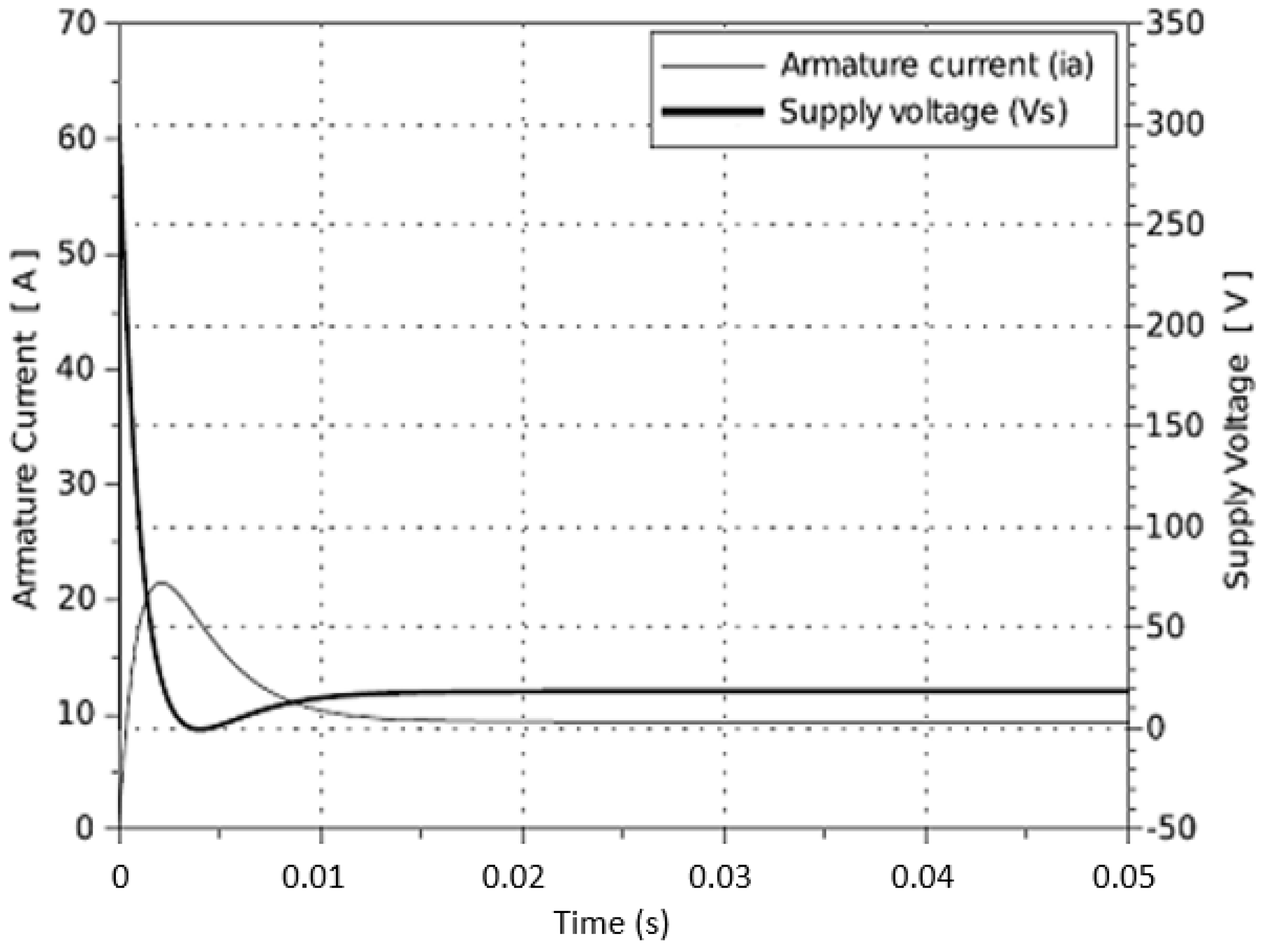
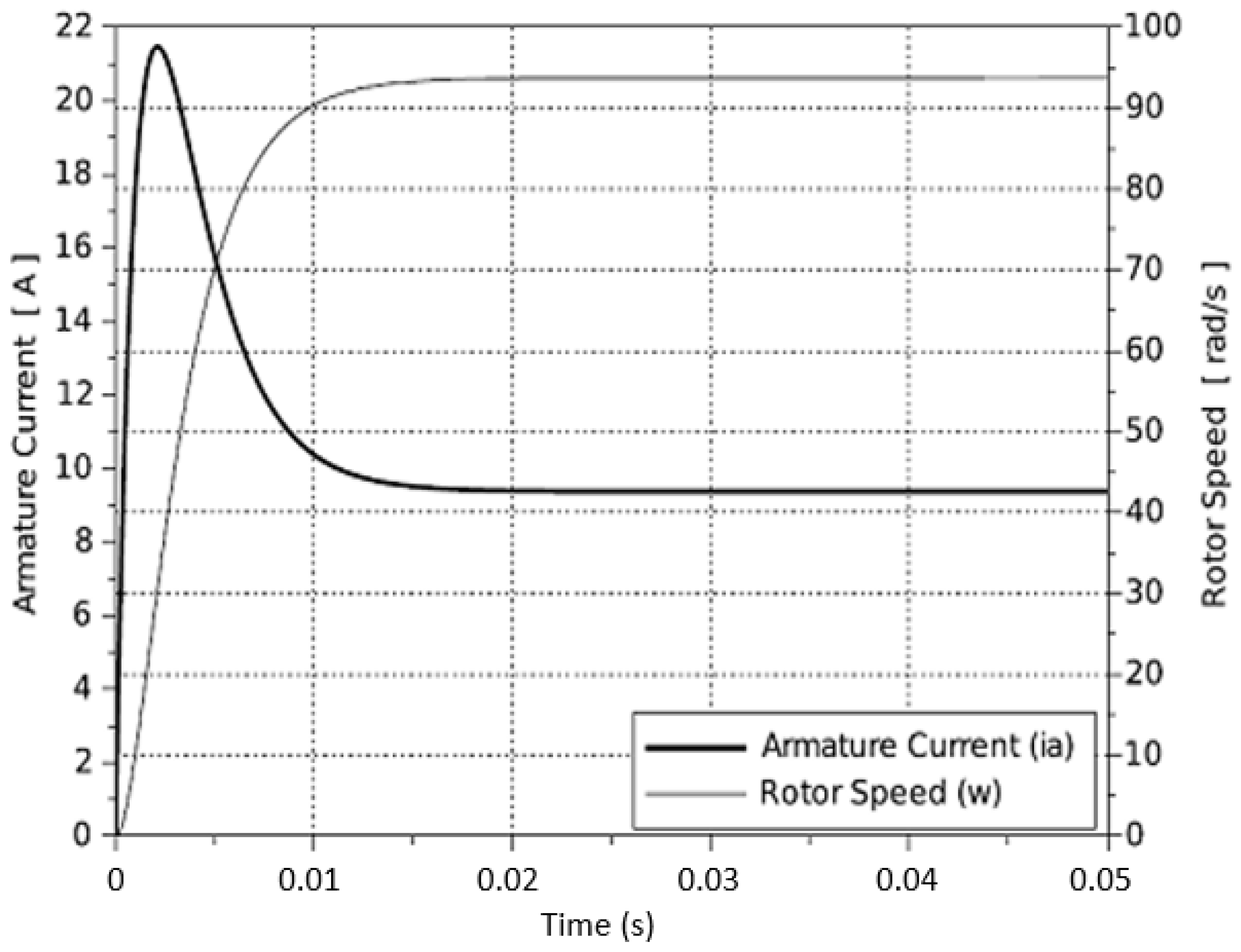
3.6. Pd Control Simulations

The closed-loop tests were run based on a negative and unitary feedback gain, as depicted in Figure 17.
Considering a no-load scenario, i.e., T L ( t ) = T L ( n ) = 0 , and initial conditions equal to zero, a desired speed of ω D = 100 rad/s was defined as the set point. Additionally, the DC motor parameters were taken from Table 2. Furthermore, the following simulation parameters were defined for the simulation: a sampling period equal to 10 μ s and trial-and-error-based controller’s gains K P = 3 and K D = 0.01 .
Figure 18 shows the controller’s output, v s ( t ) , that feeds the DC motor. Transient and steady-state responses are visualized. Moreover, the controlled variable ω ( t ) is portrayed in Figure 19. It is noticed that the closed-loop system exhibits a steady-state error of approximately 64 rad/s.

4. Conclusions, Limitations, and Future Work

The developed activity, including collaborative learning and flipped classroom techniques, is oriented to promote active learning by working in a relevant and interesting context for electrical engineering. The activity is focused on student-centered learning and seeks to keep students motivated to develop valuable disciplinary and transversal competencies, such as the mathematical modeling of an actuator widely used in industry, the design of automated control systems for motor’s angular speed, and teamwork. By completing this activity, the student will understand the main equations that model the dynamics of a DC motor, and how—when passed to the Laplace domain—they can be interconnected in a block diagram that highlights the input and output of the system. Furthermore, students will be able to evaluate the behavior of the DC motor via a purely electrical circuit with dependent sources and to simulate the operation of the motor in terms of the input (voltage), the intermediate variable (armature current), and the outputs (torque and angular speed), with a cost-free computational tool. Additionally, the computer simulations were confirmed by solving the differential equations using Euler’s numerical method in a cost-free software tool.
Upon completing the activity, students are expected to identify some findings that are attached to the development of competencies. For example, the system of differential equations describing the DC motor can be solved by using an electric circuit simulator to reinforce the understanding of the phenomenon and modeling work. In this case, the current-controlled voltage sources along with the crossed-circuit layout were a key feature in carrying out the analysis and simulation. Additionally, PD control for DC motors can be designed directly by discretizing and simultaneously solving the system of differential equations, without the need of an specialized toolbox. This fact is important to carry out the control layout in a free licensed tool such as Qucs. In addition, the dynamical system presents asymptotic stability conditions via Lyapunov’s direct method in discrete time domain. This procedure is very valuable in control engineering courses where it is required to ensure the stability of the dynamical system. Lyapunov’s stability analysis can be performed with students’ prior knowledge of complex variable and matrix algebra.
The development of this proposal included a comparison with other proposals for modeling and control of electric motors and it was observed that the inclusion of an instructional framework with skills to be developed, didactic techniques, an activities breakdown, and an implementation proposal in the context of MFDM—these are unreported elements that can reinforce the teaching–learning process.
From a methodological point of view, the study has its limitations, although this does not detract from its relevance. A control group is required to measure the impact on students, and it should have similar characteristics to those of the experimental one; for example, MFDM, the same topics reviewed, the same learning objectives, and—if possible—the same teacher. At the end of the course, the progress in the development of the three declared sub-competencies should be compared between the two groups. However, this work would be the next stage in the line of research. Another limitation is the rubric; some subjectivity is always present in the evaluation. On the other hand, the field notes of the professors are qualitative and can also be a bias in decision making and study findings.
An effort to validate the proposed activity is the rule-based system approach. An anonymous Likert scale survey was applied to seventeen undergraduate engineering students with formal knowledge on electric circuits, DC motors, and automatic control, who have participated in non-elective courses where collaborative work and flipped classroom techniques—along with a massive flexible digital approach—have been applied. A rule-based method was applied to validate the data generated from the survey. This validation approach is based on the mathematical theory of possibility that models a certain type of uncertainty. To validate the data, the procedure reported in [50] was handled. This effort included the categorization of the questions, as well as the calculation of uncertainty level, uncertainty factor, and another uncertainty factor for each category. Moreover, a decision tree with the uncertainty factor per category was generated along with conclusions to define the categories’ impacts in the survey. This development is explained in Appendix B and Appendix C.
Future work includes the implementation of the activity in an undergraduate engineering course using the Massive Flexible Digital Masterclass (MFDM), as explained in Appendix A. The learning outcomes should be evaluated with a rubric and measured in terms of grades and observed competencies. As a later activity, field-wound and brushless DC motors, as well as single-phase and three-phase alternate-current motors, could be considered, along with other control techniques and performance criteria. For more advanced undergraduate courses, a nonlinear modeling of the DC motor using a circuit simulator to analyze another dynamics of interest could be considered. By including these topics, broader aspects of undergraduate engineering courses, such as actuators, alternating current circuits, and power interfaces, could be covered.

Author Contributions

Conceptualization, A.S.; methodology, A.S.; L.C.F.-H., R.S. and R.A.R.-M.; software, A.S.; validation, A.S., Y.A.D. and C.H.-S.; formal analysis, A.S., Y.A.D. and C.H.-S.; investigation, A.S., L.C.F.-H., Y.A.D. and C.H.-S.; resources, A.S.; data curation, L.C.F.-H., Y.A.D. and C.H.-S.; writing—original draft preparation, A.S.; writing—review and editing, L.C.F.-H., Y.A.D., R.S. and R.A.R.-M.; visualization, L.C.F.-H., R.S. and R.A.R.-M.; supervision, R.S. and R.A.R.-M.; project administration, L.C.F.-H.; funding acquisition, R.A.R.-M. All authors have read and agreed to the published version of the manuscript.

Funding

This work has been supported by Consejo Nacional de Ciencia y Tecnología (CONACYT), and Tecnologico de Monterrey, México.

Acknowledgments

Authors are grateful to Tecnologico de Monterrey, School of Engineering and Science for funding the publication cost of this research.

Conflicts of Interest

The authors declare no conflict of interest.

Appendix A. Massive Flexible Digital Masterclass (MFDM)

The Massive Flexible Digital Masterclass (MFDM) model will be applied to carry out this proposal. Such method considers a virtuous scheme in which the professors in electrical engineering courses has an important recognition among colleagues and students. This flexible scheme enables the professor to teach and positively affect students nationwide without space limitations, targeting more than 300 students per class. Flexibility is one of the key elements of this model, allowing for the delivery of contents and activities to the students via asynchronous media and formats, while having either “face-to-face” or virtual interactions with the professor.
The digital nature of the MFDM model could include renowned researchers and industry experts to participate on select topics through digital masterclasses and webinars without the logistical and time constraints of an in-person course. Moreover, MFDMs focus on learning through the development of competencies, highlighted in innovative teaching–learning processes, based on active learning. The MFDM combines different didactic techniques, including flipped classroom (FC), to develop competencies, such as problem solving and teamwork. Students can learn at their own speed/time in an asynchronous manner, while engaging and discussing the concepts with the teacher during the synchronous session, thus deepening the learning process and preparing them for a hands-on experience with real-world applications of the concepts learned. Figure A1 shows the pedagogic elements of the MFDM scheme.
The expected learning benefits of the implementation of MFDMs are given as follows:
  • Strong understanding of the physical phenomena involved in an electrical engineering class.
  • Strong understanding of the relationships between the equations and the behavior of the variables of interest, such as armature current, motor torque, and angular speed.
  • Enhance the simulation skill of the students: the motor’s behavior is analyzed by means of a circuit simulator, where the effects of a specific supply voltage, load torque, and motor parameters can be studied in an agile, cheap, and reliable manner.
  • Analogy between the direct current motor and an electrical circuit, where the first one involves electrical and mechanical variables, and the second one involves only electrical variables.
  • Enhance the ability to identify, formulate, and solve electrical engineering problems.
  • Enhance the ability to apply electrical engineering design.
  • Enhance the ability to develop and conduct appropriate experimentation, analyze and interpret data, and use engineering judgment to draw conclusions.
Figure A1. Elements of the Massive Flexible Digital Masterclass (MFDM) pedagogic model.
Electronics 11 01059 g0a1

Appendix B. Questionnaire

  • The work scheme, presented in the activity’s breakdown, allows developing the transversal competence of effective communication and reasoning for complexity.
    (SA) Strongly Agree (A) Agree (N) Not sure (D) Disagree (SD) Strongly Disagree
  • The activities in session 1, students and professor, allow the development of the competency of mathematical modeling of a direct current motor dynamic.
    (SA) Strongly Agree (A) Agree (N) Not sure (D) Disagree (SD) Strongly Disagree
  • The simulation effort, individual and collaborative, along with the plenary sessions, contribute to validate the mathematical model.
    (SA) Strongly Agree (A) Agree (N) Not sure (D) Disagree (SD) Strongly Disagree
  • The flipped classroom didactic technique enables, with an adequate balance, one to carry out the sequence of activities, with the purpose of developing the declared competencies.
    (SA) Strongly Agree (A) Agree (N) Not sure (D) Disagree (SD) Strongly Disagree
  • The deployment proposal is proposed in the context of a Massive Flexible Digital Masterclass (MFDM). As a student who has participated in massive courses and some of them in remote format, do you consider this scheme adequate to develop the declared competencies?
    (SA) Strongly Agree (A) Agree (N) Not sure (D) Disagree (SD) Strongly Disagree
  • The modeling, as defined in the activity for the simulation approach, as a pure electric circuit, allows modeling the dynamics of a permanent magnet electric current motor.
    (SA) Strongly Agree (A) Agree (N) Not sure (D) Disagree (SD) Strongly Disagree
  • The activities to analyze and design the control system (flipped classroom, teamwork, simulations, and plenary wrap-up) are sufficient for understanding the relationship between automatic control and motors, as well as their importance as elements of an automatic control loop where it is required to ensure stability.
    (SA) Strongly Agree (A) Agree (N) Not sure (D) Disagree (SD) Strongly Disagree

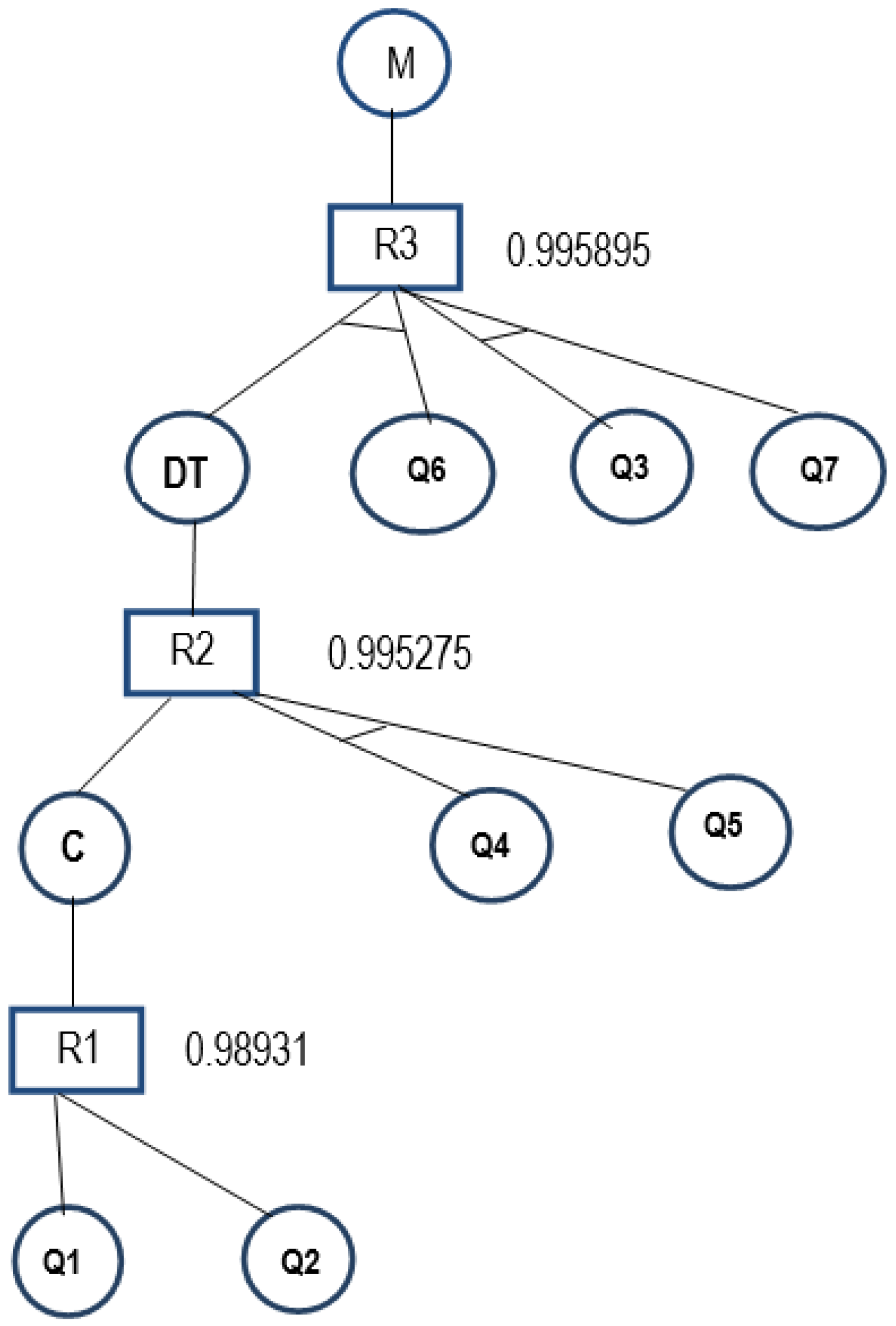
Appendix C. Survey Validation through a Rule-Based System

The following procedure was conducted to develop this expert system:
  • To validate the seven-question Likert scale survey, a ruled-based methodology, developed in [50], is applied. The following procedure was conducted to develop this expert system:
    Based on their meaning, the seven questions were categorized into three groups: competencies (C), mechatronics (M), and didactic techniques (DT), and the groups were as follows: Questions 1 and 2 in C category as C-1 and C-2, respectively; Questions 3, 6, and 7, in M, as M-1, M-2, and M-3, respectively; and Questions 4 and 5 in DT category as DT-1 and DT-2, respectively.
  • Based on [50], Table A1 was populated. In the table, U L stands for uncertainty level, U F represents the certainty factor per question, and C U F is the uncertainty factor of a category.
Table A1. Questions —categorization, frequencies, uncertainty level, and certainty factor per question and category.
QR1f1R2f2R3f3R4f4R5f5fTULUFCUF
C-10000.00010.059130.76530.17610.2740.7260.989314
C-20000.00030.17660.35380.47110.0390.961
M-10000.00000.000140.82430.17610.3680.6320.995895
M-20000.00050.29490.52930.17610.0780.922
M-30000.00010.059110.64750.29410.1430.857
DT-10030.17660.35350.29430.17610.0450.9550.995275
DT-20010.05940.235100.58820.11810.1050.895
3.
An AND/OR decision tree is presented in Figure A2, for the production rules in Equation (A1)–(A3).
C F 1 ( C ) = m a x ( C F ( Q 1 ) , C F ( Q 2 ) ) . C F ( R 1 )
C F 2 ( D T ) = m a x ( C F ( C ) , m i n ( C F ( Q 4 ) , C F ( Q 5 ) ) ) . C F ( R 2 )
C F 3 ( M ) = m a x ( m i n ( C F ( D T ) , C F ( Q 6 ) ) , m i n ( C F ( Q 3 ) , C F ( Q 7 ) ) ) . C F ( R 3 )
From the decision tree in Figure A2, based on the survey, with the categories mechatronics (M), didactic techniques (DT), and competencies (C), the decision tree presents that C F 3 = 0.91822 , which implies that mechatronics students require proper didactic techniques to improve their competencies in the teaching–learning process.
Figure A2. Decision tree for three production rules.
Electronics 11 01059 g0a2

References

  1. Román-Graván, P.; Hervás-Gómez, C.; Martín-Padilla, A.H.; Fernández-Márquez, E. Perceptions about the Use of Educational Robotics in the Initial Training of Future Teachers: A Study on STEAM Sustainability among Female Teachers. Sustainability 2020, 12, 4154. [Google Scholar] [CrossRef]
  2. Renkl, A.; Atkinson, R.K.; Maier, U.H.; Staley, R. From example study to problem solving: Smooth transitions help learning. J. Exp. Educ. 2002, 70, 293–315. [Google Scholar] [CrossRef] [Green Version]
  3. Bonwell, C.; Eison, J. Active Learning: Creating Excitement in the Classroom. In 1991 ASHE-ERIC Higher Education Reports; ERIC Clearinghouse on Higher Education: Washington, DC, USA, 1991. [Google Scholar]
  4. Pardjono, P. Active Learning: The Dewey, Piaget, Vygotsky, and Constructivist Theory Perspectives. Psychol. J. Ilmu Pendidik. 2016, 9, 105376. [Google Scholar]
  5. Prince, M. Does Active Learning Work? A Review of the Research. J. Eng. Educ. 2004, 93, 223–231. [Google Scholar] [CrossRef]
  6. Sastry, V.L.N.; Rao, K.S.; Rao, N.V.; Clee, P.; Kumari, G.R. Effective and Active Learning in Classroom Teaching through Various Methods. In Proceedings of the IEEE 4th International Conference on MOOCs, Innovation and Technology in Education (MITE), Madurai, India, 9–10 December 2016; pp. 105–110. [Google Scholar] [CrossRef]
  7. Gren, L. A Flipped Classroom Approach to Teaching Empirical Software Engineering. IEEE Trans. Educ. 2020, 63, 155–163. [Google Scholar] [CrossRef] [Green Version]
  8. Tecnológico de Monterrey. Aprendizaje Colaborativo. Vicerrectoría Académica y de Innovación Educativa. Available online: https://innovacioneducativa.tec.mx/aprendizaje-colaborativo/ (accessed on 20 May 2020). (In Spanish).
  9. DeLozier, S.J.; Rhodes, M.G. Flipped Classrooms: A Review of Key Ideas and Recommendations for Practice. Educ. Psychol. Rev. 2017, 29, 141–151. [Google Scholar] [CrossRef]
  10. Ramírez-Mendoza, R.A.; López-Guajardo, E.A. Massive Flexible Digital Masterclss Model (MFDM); Tecnologico de Monterrey: Monterrey, Mexico, 2021. [Google Scholar]
  11. Prpić, J.; Melton, J.; Taeihagh, A.; Anderson, T. MOOCs and crowdsourcing: Massive courses and massive resources. First Monday 2015, 20. [Google Scholar] [CrossRef] [Green Version]
  12. Kulkarni, C.; Cambre, J.; Kotturi, Y.; Bernstein, M.S.; Klemmer, S. Talkabout: Making Distance Matter with Small Groups in Massive Classes. In Proceedings of the 18th ACM Conference on Computer Supported Cooperative Work & Social Computing (CSCW’15), Vancouver, BC, Canada, 14–18 March 2015; pp. 1116–1128. [Google Scholar] [CrossRef] [Green Version]
  13. Zavalani, O.; Kaçani, J. Mathematical modelling and simulation in engineering education. In Proceedings of the 15th International Conference on Interactive Collaborative Learning (ICL), Villach, Austria, 26–28 September 2012; pp. 1–5. [Google Scholar] [CrossRef]
  14. Litwin, P.; Stadnicka, D. Computer Modeling and Simulation in Engineering Education: Intended Learning Outcomes Development. In Advances in Manufacturing II. MANUFACTURING; Hamrol, A., Grabowska, M., Maletic, D., Woll, R., Eds.; Lecture Notes in Mechanical Engineering; Springer: Cham, Switzerland, 2019. [Google Scholar]
  15. Zill, D.G. Advanced Engineering Mathematics; Jones & Bartlett Learning: Burlington, MA, USA, 2017. [Google Scholar]
  16. Mohan, N.; Underland, T.M. Power Electronics: Converters, Applications, and Design; John Wiley & Sons: Hoboken, NJ, USA, 2003; pp. 377–379. [Google Scholar]
  17. Sabir, M.M.; Khan, J. Optimal design of PID controller for the speed control of DC motor by using metaheuristic techniques. Adv. Artif. Neural Syst. 2014, 2014, 126317. [Google Scholar] [CrossRef] [Green Version]
  18. Hughes, A.; Drury, B. Electric Motors and Drives: Fundamentals, Types and Applications; Newnes: Oxford, UK, 2013; pp. 73–91. [Google Scholar]
  19. Aung, W.P. Analysis on modeling and simulink of DC motor and its driving system used for wheeled mobile robot. World Acad. Sci. Eng. Technol. Open Sci. Int. J. Electr. Comput. Eng. 2007, 1, 299–306. [Google Scholar]
  20. Said, A.; Rodriguez-Leal, E.; Soto, R.; Gordillo, J.L.; Garrido, L. Decoupled Closed Form Solution for Humanoid Lower Limb Kinematics. Math. Probl. Eng. 2015, 2015, 1–14. [Google Scholar] [CrossRef]
  21. Hearn, C.; Weeks, S.; Thompson, R.C.; Chen, D. Electric vehicle modeling utilizing DC motor equations. In Proceedings of the IEEE/ASME International Conference on Advanced Intelligent Mechatronics (AIM), Montreal, QC, Canada, 6–9 July 2010; pp. 670–675. [Google Scholar]
  22. Hwang, Y.-R.; Huang, S.-Y. System identification and integration design of an air/electric motor. Energies 2013, 6, 921–933. [Google Scholar] [CrossRef] [Green Version]
  23. Bitar, Z.; Samith, A.J.; Khamis, I. Modeling and simulation of series DC motors in electric car. Energy Procedia 2014, 50, 460–470. [Google Scholar] [CrossRef] [Green Version]
  24. Wu, W. DC motor parameter identification using speed step responses. Model. Simul. Eng. 2012, 2012, 189757. [Google Scholar] [CrossRef] [Green Version]
  25. Arduino. Available online: https://www.arduino.cc/ (accessed on 20 January 2020).
  26. Raspberry, P. The Raspberry Pi Foundation. Available online: https://www.raspberrypi.org/ (accessed on 22 January 2020).
  27. Abut, T. Modeling and Optimal Control of a DC Motor. Int. J. Eng. Trends Technol. 2016, 32, 146–150. [Google Scholar] [CrossRef]
  28. Sinha, N.K.; Dicenzo, C.D.; Szabados, B. Modeling and Optimal Control of a DC Motor. Modeling of DC motors for control applications. IEEE Trans. Ind. Electron. Control Instrum. 1974, IECI-21, 84–88. [Google Scholar] [CrossRef]
  29. Guldemir, H. Sliding mode speed control for DC drive systems. Math. Comput. Appl. 2003, 8, 377–384. [Google Scholar] [CrossRef] [Green Version]
  30. Bhushan, B.; Singh, M. Adaptive control of DC motor using bacterial foraging algorithm. Appl. Soft Comput. 2011, 11, 4913–4920. [Google Scholar] [CrossRef]
  31. Yelamarthi, K.; Drake, E.; Prewett, M. An Instructional Design Framework to Improve Student Learning in a First-Year Engineering Class. J. Inf. Technol. Educ. Innov. Pract. 2016, 15, 195–222. [Google Scholar] [CrossRef] [Green Version]
  32. Villarroel, R.; Cornide-Reyes, H.; Munoz, R.; Barcelos, T. Flipped classroom + plickers, and experience to propitiate collaborative learning in software engineering. In Proceedings of the 36th International Conference of the Chilean Computer Science Society, Arica, Chile, 16–20 October 2017; pp. 1–7. [Google Scholar] [CrossRef]
  33. Soares, F.; de Moura Oliveira, P.B.; Leao, C.P. Your turn to learn—Flipped classroom in automation courses. In Lecture Notes in Electrical Engineering, Proceedings of the 14th APCA International Conference on Automatic Control and Soft Computing, Bragança, Portugal, 1–3 July 2020; Springer: Cham, Switzerland, 2020; Volume 695, p. 695. [Google Scholar] [CrossRef]
  34. Yan, J.; Li, L.; Yin, J.; Nie, Y. A comparison of flipped and traditional classroom learning: A case study in mechanical engineering. Int. J. Eng. Educ. 2018, 34, 1876–1887. [Google Scholar]
  35. Zamarron-Ramirez, A.; Arjona, M. Detection of Stator-Winding Turn-to-Turn Faults in Induction Motors, Based on Virtual Instrumentation. Int. J. Electr. Eng. Educ. 2010, 47, 63–72. [Google Scholar] [CrossRef]
  36. Fuertes, J.J.; Domínguez, M.; Prada, M.A.; Alonso, S.; Morán, A. A Virtual Laboratory of D.C. Motors for Learning Control Theory. Int. J. Electr. Eng. Educ. 2013, 50, 172–187. [Google Scholar] [CrossRef]
  37. Reis, A.; da Costa, F.H.; Xavier, G.L.; Alvarenga, E.B.; de Oliveira, J.C.; Guimarães, G.C. Comparative Performance Analysis of a Controlled D.C. and A.C. Motor Which Emulates Wind Turbines for Teaching and Research Purposes. Int. J. Electr. Eng. Educ. 2014, 51, 146–161. [Google Scholar] [CrossRef]
  38. Reck, R.M.; Sreenivas, R.S. Developing an Affordable and Portable Control Systems Laboratory Kit with a Raspberry Pi. Electronics 2016, 5, 36. [Google Scholar] [CrossRef] [Green Version]
  39. Chasiotis, I.D.; Karnavas, Y.L. A computer aided educational tool for design, modeling, and performance analysis of Brushless DC motor in post graduate degree courses. Comput. Appl. Eng. Educ. 2018, 24, 749–767. [Google Scholar] [CrossRef]
  40. Sami, S.; Obaid, Z.A.; Muhssin, M.T.; Hussain, A.N. Detailed modelling and simulation of different DC motor types for research and educational purposes. Int. J. Power Electron. Drive Syst. 2021, 12, 703–714. [Google Scholar] [CrossRef]
  41. Tudić, V.; Kralj, D.; Hoster, J.; Tropčić, T. Design and Implementation of a Ball-Plate Control System and Python Script for Educational Purposes in STEM Technologies. Sensors 2022, 22, 1875. [Google Scholar] [CrossRef]
  42. Gay, L.R.; Mills, G.E.; Airasian, P. Educational Research: Competencies for Analysis and Applications; Merrill Prentice Hall: Columbus, OH, USA, 2006. [Google Scholar]
  43. Trochim, W.; Donnelly, J. The Research Methods Knowledge Base; Thomson: Mason, OH, USA, 2007. [Google Scholar]
  44. Hernández, R.; Fernández, C.; Baptista, M. Metodología de la Investigación; McGraw-Hill: Mexico City, Mexico, 2014. [Google Scholar]
  45. He, X.; Ju, Y.; Liu, Y.; Zhang, B. Cloud-Based Fault Tolerant Control for a DC Motor System. J. Control Sci. Eng. 2017, 2017, 5670849. [Google Scholar] [CrossRef]
  46. Qucs. Quite Universal Circuit Simulator. Available online: http://qucs.sourceforge.net/ (accessed on 30 January 2020).
  47. Nakamura, S. Métodos Numéricos Aplicados con Software; Prentice Hall: Naucalpan, Mexico, 1992; pp. 292–295. ISBN 0-13-041047-0. [Google Scholar]
  48. Burden, R.; Faires, J. Numerical Analysis; Thomson Learning: Boston, MA, USA, 2002; pp. 266–273. ISBN 978-0-538-73351-9. [Google Scholar]
  49. Scilab. Scilab Enterprises. Available online: http://www.scilab.org/ (accessed on 20 January 2020).
  50. Espino-Román, P.; Davizon-Castillo, Y.; Olaguez-Torres, E.; Gamez-Wilson, J.; Said, A.; Hernandez-Santos, C. Development of a rule based system to validate an educational survey in a Likert scale. DYNA 2020, 95, 572. [Google Scholar] [CrossRef]
Figure 1. Competency-oriented flowchart. Modeling and validation.
Electronics 11 01059 g001
Figure 2. DC motor block diagram.
Electronics 11 01059 g002
Figure 3. Equivalent circuit of a DC motor. Pure electrical circuit with 2 meshes.
Electronics 11 01059 g003
Figure 4. Equivalent circuit of a DC motor using Qucs simulator and a constant voltage supply of v s = 100 V.
Electronics 11 01059 g004
Figure 5. A simulation using Qucs of the armature current i a ( t ) under no-load conditions when using a supply voltage of v s = 100 V.
Electronics 11 01059 g005
Figure 6. A simulation using Qucs of the rotor speed ω ( t ) under no-load conditions when using a supply voltage of v s = 100 V.
Electronics 11 01059 g006
Figure 7. A simulation using Scilab of a constant supply voltage of v s = 100 V and the resultant armature current i a ( t ) under no-load conditions.
Electronics 11 01059 g007
Figure 8. A simulation using Scilab of the armature current i a ( t ) and rotor speed ω ( t ) under no-load conditions when using a constant supply voltage of v s = 100 V.
Electronics 11 01059 g008
Figure 9. A simulation using Qucs of the armature current, i a ( t ) , under no-load conditions, when using a PWM supply voltage with a peak value of 100 V and a duty cycle of 50 % .
Electronics 11 01059 g009
Figure 10. A simulation using Qucs of the rotor speed ω ( t ) under no-load conditions when using a PWM supply voltage with a peak value of 100 V and a duty cycle of 50 % .
Electronics 11 01059 g010
Figure 11. Simulation (Scilab) under no-load conditions, with a PMW supply voltage of amplitude equal to 100 V and a duty cycle of 50 % . The dependent variable is i a ( t ) .
Electronics 11 01059 g011
Figure 12. Simulation (Scilab) under no-load conditions, with a PMW supply voltage of amplitude equal to 100 V and a duty cycle of 50 % . The dependent variable is ω ( t ) .
Electronics 11 01059 g012
Figure 13. Load test results in Qucs for i a ( t ) . The load torque = 5 Nm.
Electronics 11 01059 g013
Figure 14. Load test results in Qucs for ω ( t ) . The load torque = 5 Nm.
Electronics 11 01059 g014
Figure 15. Load test results in Scilab for i a ( t ) , with a load torque = 5 Nm.
Electronics 11 01059 g015
Figure 16. Load test results in Scilab for ω ( t ) , with a load torque = 5 Nm.
Electronics 11 01059 g016
Figure 17. Closed-loop simulated system with a PD controller and with a negative and unitary feedback signal.
Electronics 11 01059 g017
Figure 18. Armature current and supplied voltage in no-load conditions with a speed controller using K P = 3 , K D = 0.01 , and ω D = 100 rad/s.
Electronics 11 01059 g018
Figure 19. ω ( t ) and i a ( t ) in no-load conditions with a set point of ω D = 100 rad/s.
Electronics 11 01059 g019
Table 1. State-of-the-art mathematical modeling, simulation, and control systems of electric motors for teaching/research in engineering academic programs.
ManuscriptContributionSoftwareMathematical ModelingControl Strategy
Zamarrón and Arjona (2010) [35]Virtual instrumentation system for stator turn-to-turn winding-fault detection to prevent unexpected downtime or severe damage to induction motors (suitable for industry and academy)LabVIEWState–spaceFault detection
Fuertes et al. (2013) [36]Modular equipment simulation to control a DC motor educational set. Part of a remote laboratory of automatic controlJAVACoupled ordinary differential equationsPID
Reis, et al. (2014) [37]Modeling and control of motors that emulate wind turbines. Comparison of two approaches with DC and AC motors.LabVIEWCoupled ordinary differential equationsFrequency response
Reck and Sreenivas (2016) [38]Affordable and portable laboratory kit design for control systems courses (DC motor plus Furuta inverted pendulum).Raspberry pi and MATLABPhysical and electric characteristics, step and frequency responsePID control
Chasiotis and Karnavas (2018) [39]Educational platform to study brushless DC motor design and performance analysisMATLABDynamic equations from physical propertiesNot reported
Samil, et al. (2021) [40]Virtual laboratory of DC motors modelingMATLABDynamic equations from physical principlesNot reported
Tudic, et al. (2022) [41]Design, manufacturing, assembly, programming, and optimization of a nonlinear mechatronic ball–plate prototype as a laboratory platform for engineering education.PythonSystem IdentificationPID control
Table 2. DC motor parameters for the case study simulation.
ParameterDescriptionQuantityUnit
Rarmature resistance1ohms
Larmature inductance10mH
Barmature friction10,000 μ N ms
Jarmature J (rotor)100 μ kg m 2
Kelectromechanical constant0.1Wb
Publisher’s Note: MDPI stays neutral with regard to jurisdictional claims in published maps and institutional affiliations.

