
Optimization Approach for the Aggregation of Flexible Consumers


Abstract
:1. Introduction
2. Flexible Consumers
- Ramp-up power rates.
- Ramp-down power rates.
- Response time when a deformation profile is activated.
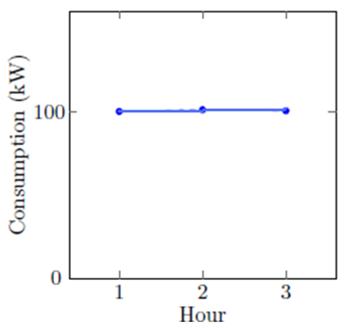
- Power consumption on each time slot.
- Maximal power on each time slot: so we cannot increase the consumption beyond this maximum.
- Minimal power on each time slot: so we cannot go below this minimum.
- The minimal duration of interruption: The deformation profile, if applied, must last at least for a minimum time.
- The maximal duration of interruption.
- Delay between two interruptions: It is the time to wait between two consecutive interruptions.
- The maximal number of interruptions done during the period: for example, interrupting a cold room more than five times during ten consecutive hours is banned.
- The maximal interruption duration: For example, stopping a cold room for more than five consecutive hours is banned.
- Maximal cumulated interrupted volume: The cumulated volume (energy) to be interrupted must not exceed a maximum value.
- Exclusive activation between a set of resources: this is useful for some consumers who do not want to interrupt more than one resource at the same time.
- The maximal number of interruptions on a set of resources.
- The maximal duration of interruption on a set of resources.
- The maximal cumulated interrupted volume on a set of resources.
3. Deformation Profiles
- Not more than one deformation profile can be active on a flexible resource at the same time.
- There is a downtime after applying a deformation profile during which no other deformations can be applied.
- When deformation is applied on a flexible resource, the customer should be paid to compensate for the inconvenience caused.
- The start of the segment: UnitStartTime .
- The end of the segment: UnitStartTime .
- The value “ValueStart” at the beginning of the segment in percentage.
- The value “ValueEnd” at the end of the segment in percentage.
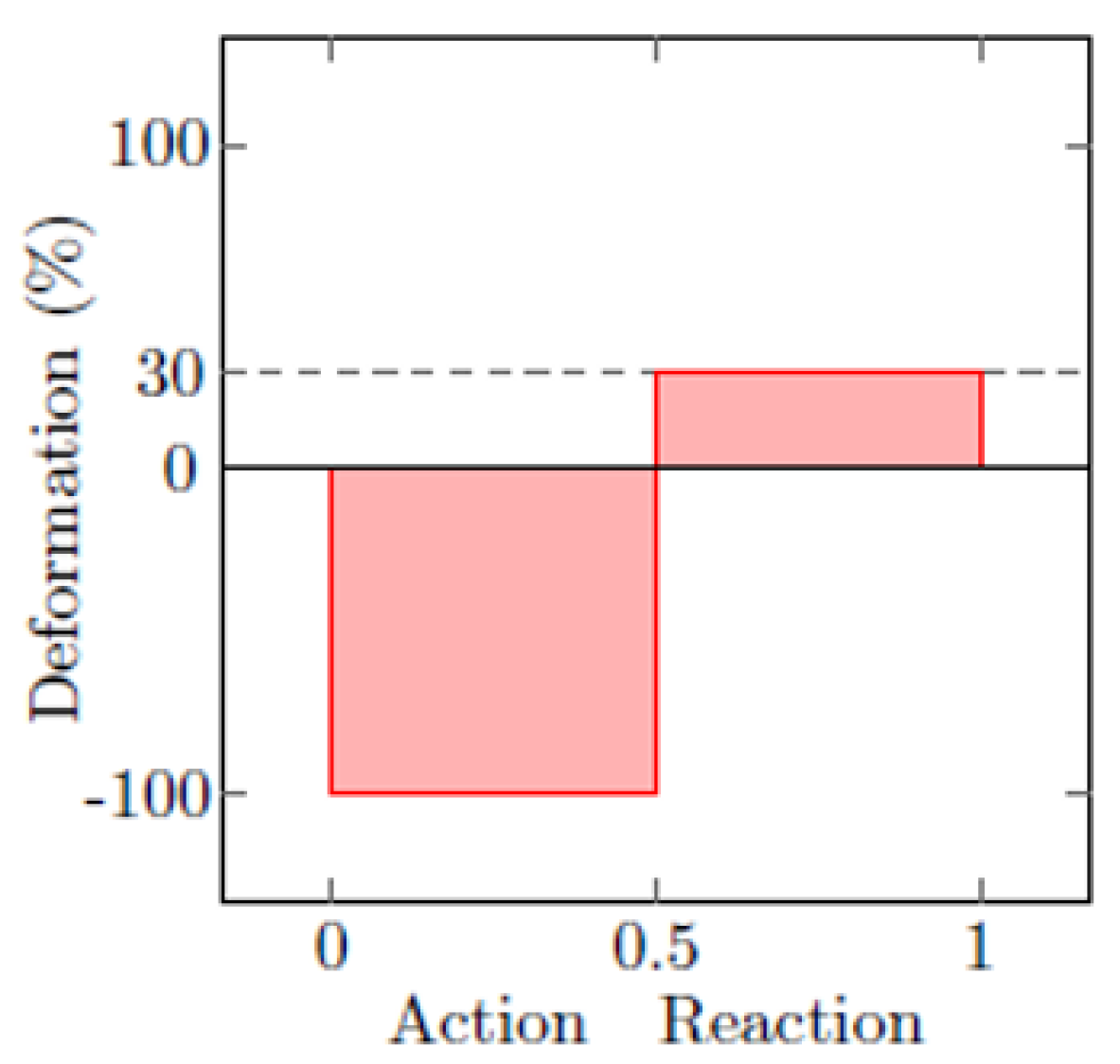
- The type of the segment: Action or Reaction.
- A value V(t) is calculated as a linear interpolation between ValueStart and ValueEnd of the segment after stretching.
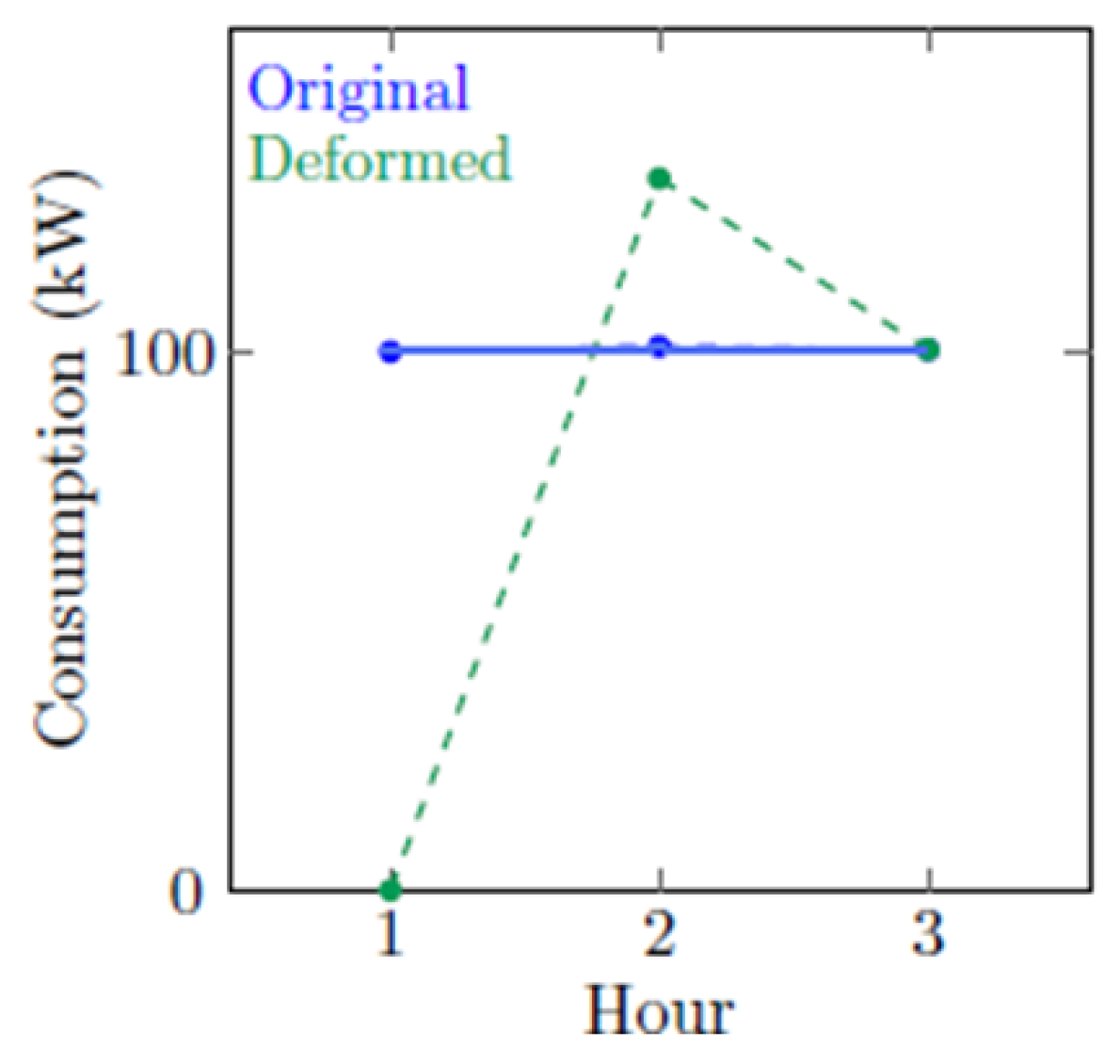
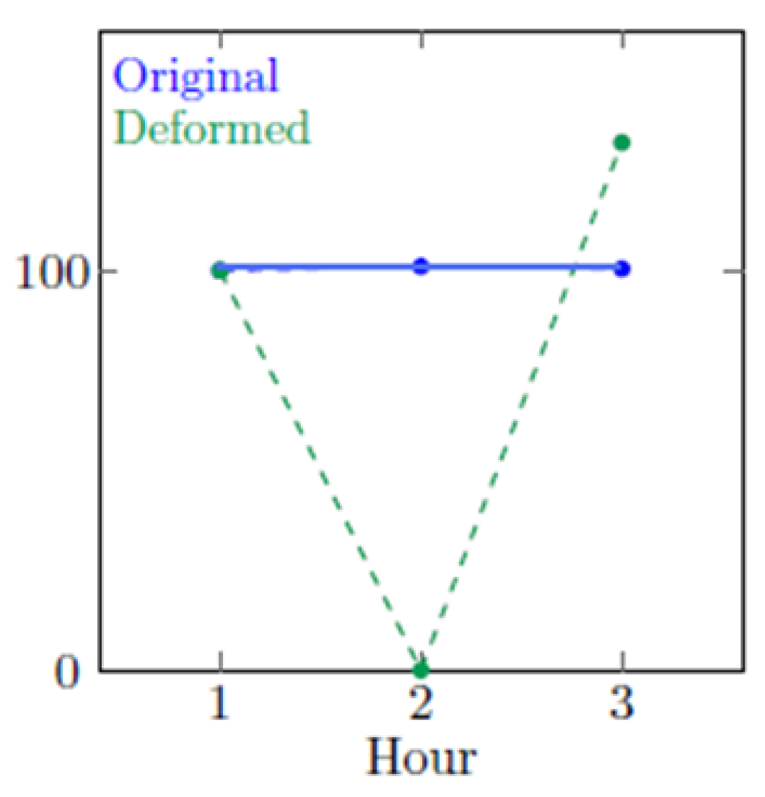
- If the segment is of type Action and if : in this case, the consumption C(t) will be increased:
- If the segment is of type Action and if : in this case, the consumption C(t) will be decreased:
- If the segment is of type Reaction, the interrupted energy during the Action period will be compensated during the Reaction period as follows:
4. Flexibility Aggregation and Price Signals
5. Problem Formulation: MILP
- T: Set of time steps covering the time horizon.
- T_PROFILE: Duration in time steps for stretched deformation profile. This set contains unique elements.
- SUB_PERIOD: List of sub-periods. Each sub-period is defined over a set of time periods.
- MAP_SUB_T (s, t): s is a sub-period, and t is a time step. This map is defined if the t is a part of the sub-period s.
- RESOURCE: Set of flexible assets to interrupt.
- MIN_OFFTIME (res): Minimum waiting time between two interruptions for the flexible asset res.
- RICH_DEFORMATION_PROFILE: A set of enriched deformation profiles (stretched deformation profiles). Each one (called rdp) is linked to only one asset. Each rdp has a duration. An enriched deformation profile is computed for a flexible resource, a normalized deformation profile, and a duration.
- MAP_RESOURCE_RDP (res, rdp): is defined iif the asset res is linked to the deformation profile rdp. A rdp is related to only one resource, but a resource can be linked to many rdp.
- RDP_DURATION (rdp): Duration of the rdp.
- DEVIATION (rdp, t, t_profile): The impact, in volume, on each time step, if rdp is activated (the effect might be negative or positive) starting from t.
- ALLOW (rdp, t): Binary parameter. It has one if rdp can be activated starting from t.
- OPP_VALUE (rdp, t): The revenue we can get if rdp is activated starting from t.
- COUPLING_CNSTR: Set of coupling constraints.
- MAP_COUPLING_RES (cc, res): Is defined iif the asset res is involved in the coupling constraint cc.
- SUB_MAX_NUM_CALLS (s, cc): Gives the value of maximum calls for the constraint cc during the subperiod s.
- SUB_MAX_DUR_CALLS (s, cc): Gives the maximum allowed duration for all resources belonging to coupling constraint cc and during the sub period s.
- SUB_MAX_VOL_CALLS (s, cc): Gives the maximum allowed volume to be interrupted for all assets belonging to the coupling constraint cc and during the sub period s.
- IS_EXCLUSIVE (s, cc): Binary parameter. One of the coupling constraints cc is exclusive: It means that only one asset could be activated during the sub period s of the coupling constraint cc or 0 otherwise.
- EXCLU_IMPACT (rdp, t, rdp2, tt) is defined if different assets linked to deformations rdp and rdp2, respectively, are mutually exclusive when activated on t (tt, respectively). This parameter will ensure that for an exclusive constraint cc, only one asset can be called at each time belonging to the sub-period of cc.
- TARGET_VOL_T (t): The target volume to be interrupted/consumed (negative or positive) for each time step.
- Penalties: The penalty used in our work is defined as a linear piecewise function for each time step with increasing slopes (so this function is convex).
- SEGM: Set of segments. Each segment represents a part of the penalty function (see Table 1).
- SEGM_PENALTY_UP_T (t, segm): Gives the penalty in EUR/kWh associated with the segment segm for the period t. This is the penalty to be used for the excess volume.
- SEGM_PENALTY_LO_T (t, segm): Gives the penalty in EUR/kWh associated with the segment segm for the period t. This is the penalty to be used for the missing volume.
- CALL (rdp, t): Binary variable; its value will be set to 1 if the rdp is activated (the asset’s load associated to the rdp is chosen to be deformed), 0 otherwise.
- MISMATCH_UP (t): Excess volume to the target by time step.
- MISMATCH_LO (t): Missing volume to the target by time step.
- SEG_MISM_UP (t, segm): The excess volume by time step and segment. This is important to ensure that we apply the correct penalty factor by segment.
- SEG_MISM_LO (t, segm): The missing volume by time step and segment.
- (1)
- For each time step t, we cannot choose a flexible asset to interrupt if this is not allowed.
- (2)
- For each coupling constraint cc, the number of activations of deformations for all periods belonging to the sub-period of cc must be less than the bound.
- (3)
- For each coupling constraint cc, the maximum duration of interruptions defined for the constraint cc and for the sub period s must be respected. gives the intersection ratio between a time step t and a subperiod s.
- (4)
- The maximum volume defined for the sub period s of the coupling constraint cc must be respected.
- (5)
- For an exclusive constraint cc, only one flexible asset could be called during the sub-period of cc.
- (6)
- This constraint aims to respect the minimum waiting time between two activations of a flexible asset.
- (7)
- For each time step and each flexible asset, only one rdp can be activated.For the dispatch mode, some additional equations must be taken into consideration:
- (8)
- This constraint aims to respect the target volume. The two variables and represent the gap to the target (UP for the excess volume and LO for the lack volume). They are penalized in the objective function to be minimized.
- (9)
- The sum of excess volume on all time steps and all segments should equal the sum of the entire extra volume. Using this constraint and the objective function, the excess volume will be dispatched correctly between segments (and respect the penalty linear piecewise function).
- (10)
- The sum of lack volume on all time steps and all segments should be equal to the sum of the entire lack volume.
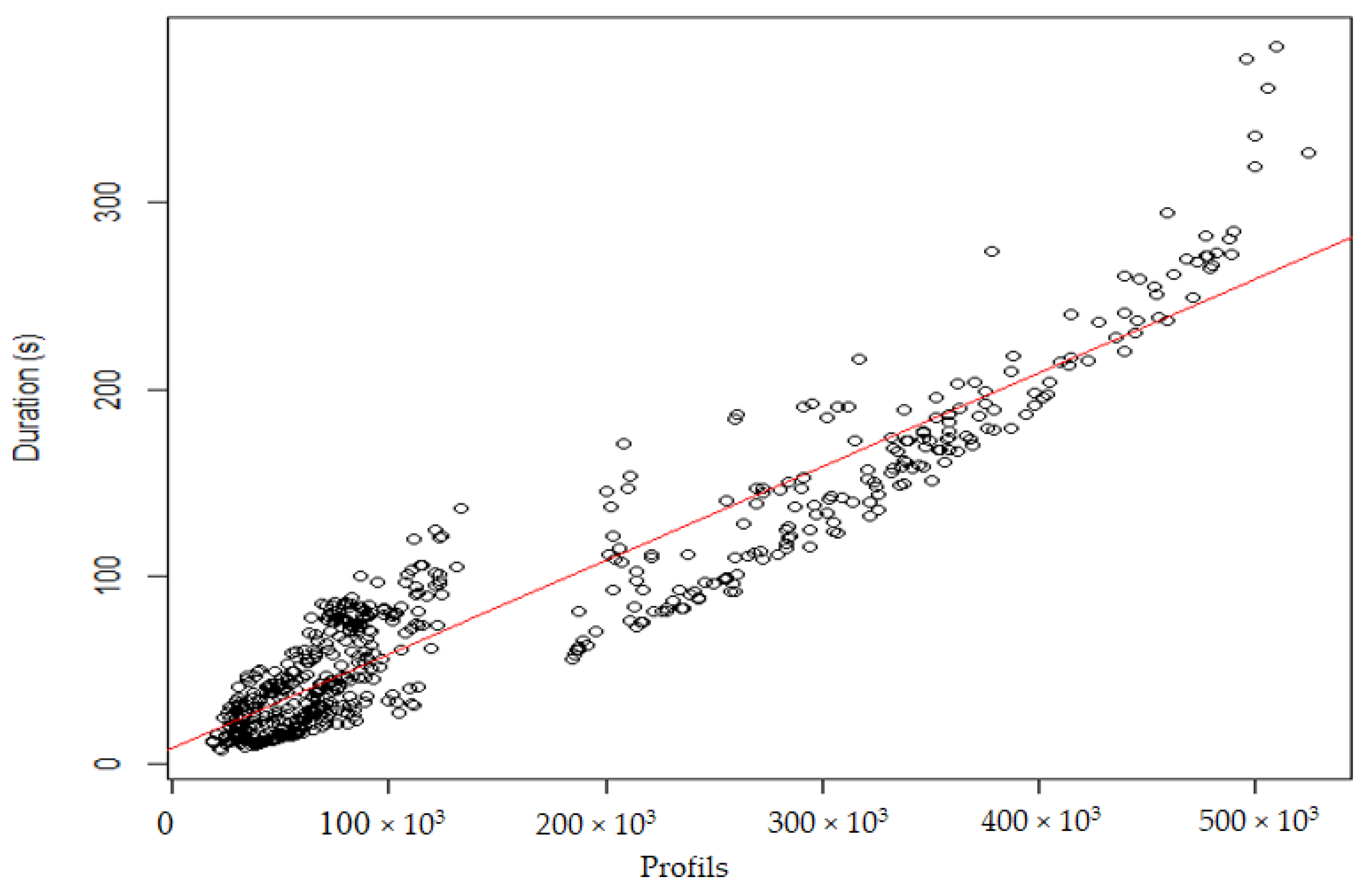
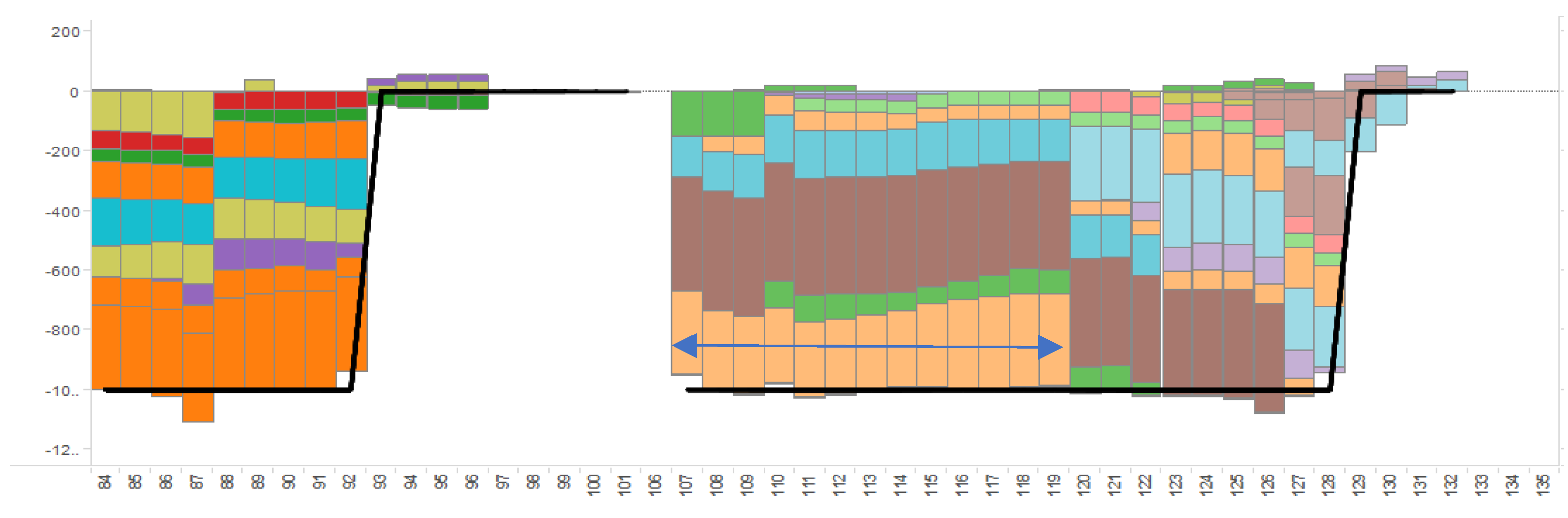
6. Experimental Results
7. Conclusions and Perspectives
Author Contributions
Funding
Institutional Review Board Statement
Informed Consent Statement
Conflicts of Interest
References
- Henderson, J.; Sen, A. The Energy Transition: Key Challenges for Incumbent and New Players in the Global Energy System; No. 01. OIES Paper: ET; The Oxford Institute for Energy Studies: Oxford, UK, 2021. [Google Scholar]
- Kalghatgi, G. Challenges of energy transition needed to meet decarbonization targets set up to address climate change. J. Automot. Saf. Energy 2020, 11, 276. [Google Scholar]
- Paterakis, N.; Erdinç, O.; Catalão, J.P.S. An overview of Demand Response: Key-elements and international experience. Renew. Sustain. Energy Rev. 2017, 69, 871–891. [Google Scholar] [CrossRef]
- Zehir, M.A.; Bagriyanik, M. Demand side management by controlling refrigerators and its effects on consumers. Energy Convers. Manag. 2012, 64, 238–244. [Google Scholar] [CrossRef]
- Kirby, B.; Hirst, E. Load as a Resource in Providing Ancillary Services; Technical Report; Oak Ridge National Labortory: Oak Ridge, TN, USA, 1999. [Google Scholar]
- Dethlefs, T.; Beewen, D.; Preisler, T.; Renz, W. A consumer-orientated architecture for distributed demand-side-optimization. In Proceedings of the 28th EnviroInfo Conference, Oldenburg, Germany, 10–12 September 2014. [Google Scholar]
- Sebastian, M.; Marti, J.; Lang, P. Evolution of DSO control centre tool in order to maximize the value of aggregated distributed generation in smart grid. In Proceedings of the 2008 CIRED Seminar: SmartGrids for Distribution, Frankfurt, Germany, 23–24 June 2008. Paper Number 0034. [Google Scholar] [CrossRef] [Green Version]
- Aalami, H.A.; Moghaddam, M.P.; Yousefi, G.R. Demand response modeling considering interruptible/curtailable loads and capacity market programs. Appl. Energy 2010, 87, 243–250. [Google Scholar] [CrossRef]
- Palensky, P.; Dietrich, D. Demand side management: Demand response, intelligent energy systems, and smart loads. IEEE Trans. Ind. Inform. 2011, 7, 381–388. [Google Scholar] [CrossRef] [Green Version]
- Esnaola-Gonzalez, I.; Jelić, M.; Pujić, D.; Diez, F.; Tomašević, N. An AI-powered system for residential demand response. Electronics 2021, 10, 693. [Google Scholar] [CrossRef]
- Habeeb, S.A.; Tostado-Véliz, M.; Hasanien, H.M.; Turky, R.A.; Meteab, W.K.; Jurado, F. DC Nanogrids for integration of demand response and electric vehicle charging infrastructures: Appraisal, optimal scheduling and analysis. Electronics 2021, 10, 2484. [Google Scholar] [CrossRef]
- Brusco, G.; Burgio, A.; Menniti, D.; Pinnarelli, A.; Sorrentino, N.; Scarcello, L. An energy box in a cloud-based architecture for autonomous demand response of prosumers and prosumages. Electronics 2017, 6, 98. [Google Scholar] [CrossRef] [Green Version]
- Peeters, E.; Belhomme, R.; Batlle, C.; Bouffard, F.; Karkkainen, S.; Six, D.; Hommelberg, M. ADDRESS: Scenarios and architecture for active demand development in the smart grids of the future. In Proceedings of the 2009 CIRED 20th International Conference on Electricity Distribution, Prague, Czech Republic, 8–11 June 2009. Paper Number 0406. [Google Scholar] [CrossRef] [Green Version]
- Pallonetto, F.; De Rosa, M.; Milano, F.; Finn, D.P. Demand response algorithms for smart-grid ready residential buildings using machine learning models. Appl. Energy 2019, 239, 1265–1282, ISSN 0306-2619. [Google Scholar] [CrossRef]
- Lopes, F.; Algarvio, H. Demand response in electricity markets: An overview and a study of the price-effect on the Iberian daily market. In Electricity Markets with Increasing Levels of Renewable Generation: Structure, Operation, Agent-Based Simulation, and Emerging Designs; Lopes, F., Coelho, H., Eds.; Springer: Cham, Switzerland, 2018. [Google Scholar] [CrossRef]
- Tan, Z.; Fan, W.; Li, H.; De, G.; Ma, J.; Yang, S.; Ju, L.; Tan, Q. Dispatching optimization model of gas-electricity virtual power plant considering uncertainty based on robust stochastic optimization theory. J. Clean. Prod. 2020, 247, 119106. [Google Scholar] [CrossRef]
- Pourghaderi, N.; Fotuhi-Firuzabad, M.; Moeini-Aghtaie, M.; Kabirifar, M. Commercial demand response Programs in bidding of a technical virtual power plant. IEEE Trans. Ind. Inform. 2018, 14, 5100–5111. [Google Scholar] [CrossRef]
- Sheble, G.B.; Fahd, G.N. Unit commitment literature synopsis. IEEE Trans. Power Syst. 1994, 9, 763–773. [Google Scholar] [CrossRef]
- Tang, W.-J.; Yang, H.-T. Optimal operation and bidding strategy of a virtual power plant integrated with energy storage systems and elasticity demand response. IEEE Access 2019, 7, 79798–79809. [Google Scholar] [CrossRef]
- Biegel, B.; Andersen, P.; Stoustrup, J.; Madsen, M.B.; Hansen, L.H.; Rasmussen, L.H. Aggregation and control of flexible consumers: A real life demonstration. In IFAC Proceedings Volumes, Proceedings of the 19th IFAC World Congress, Cape Town, South Africa, 24–29 August 2014, 1st ed.; IFAC Workshop Series; IFAC Publisher: New York, NY, USA, 2014; Volume 19, pp. 9950–9955. [Google Scholar]
- Kaddah, R.; Kofman, D.; Mathieu, F.; Pioro, M. Advanced demand response solutions for capacity markets. In Proceedings of the IEEE International Conference on Innovations in Information Technology, Dubai, United Arab Emirates, 1–3 November 2015; pp. 23–28. [Google Scholar]
- Saha, S.; Ravi, N.; Hreinsson, K.; Baek, J.; Scaglione, A.; Johnson, N.G. A secure distributed ledger for transactive energy: The Electron Volt Exchange (EVE) blockchain. Appl. Energy Part A 2021, 282, 116208, ISSN 0306-2619. [Google Scholar] [CrossRef]
- Al Zahr, S.; Doumith, E.A.; Forestier, P. Advanced demand response considering modular and deferrable loads under time-variable rates. In Proceedings of the IEEE GLOBECOM Global Communications Conference, Singapore, 4–8 December 2017. [Google Scholar] [CrossRef]
- Eurelectric. Designing Fair and Equitable Market Rules for Demand Response Aggregation; A Eurelectric Paper; Eurelectric: Brussels, Belgium, 2015. [Google Scholar]
- Hromkovic, J.; Kralovic, R.; Kralovic, R. Information complexity of online problems. In Mathematical Foundations of Computer Science 2010, Proceedings of the 35th International Symposium on Mathematical Foundations of Computer Science (MFCS 2010), Brno, Czech Republic, 23–27 August 2010; Volume 6281 of Lecture Notes in Computer Science; Springer: Berlin/Heidelberg, Germany; pp. 24–36.
- GAMS Development Corporation. General Algebraic Modeling System (GAMS), Fairfax, VA, USA. Available online: https://www.gams.com/download/ (accessed on 31 January 2022).

| Segment | Threshold | Penalty | Description |
|---|---|---|---|
| 1 | 0.1 | 0 | If the gap to the target = 0.1 → penalty = 0.1 × 0 = 0 |
| 2 | 0.5 | 5 | If the gap to the target = 0.5 → penalty = 0.1 × 0 + 0.4 × 5. |
| 3 | 2 | 20 | If Gap to the target = 1.8 → penalty = 0.1 × 0 + 0.4 × 5 + 1.3 × 20.In fact, the gap is dispatched on three segments (1.8 = 0.1 + 0.5 + 1.3) |
| Set of Instances | Min Assets | Max Assets | Min # Profiles | Max # Profiles | Mean Time—MILP |
|---|---|---|---|---|---|
| 1 | 56 | 246 | 20,540 | 91,928 | 46 s |
| 2 | 51 | 241 | 28,992 | 124,111 | 44 s |
| 3 | 51 | 246 | 18,320 | 92,319 | 22 s |
| 4 | 51 | 250 | 25,537 | 133,438 | 62 s |
| 5 | 502 | 994 | 185,891 | 366,132 | 132 s |
| 6 | 501 | 997 | 245,885 | 523,899 | 215 s |
| Set of instances | Min Assets | Max Assets | Min # Profiles | Max # Profiles | Mean Time—MILP |
|---|---|---|---|---|---|
| 1 | 50 | 250 | 26,038 | 473,758 | 157 s |
| 2 | 50 | 250 | 185,083 | 1,111,575 | 634 s |
| 3 | 500 | 1000 | 283,576 | 613,296 | 672 s |
Publisher’s Note: MDPI stays neutral with regard to jurisdictional claims in published maps and institutional affiliations. |
© 2022 by the authors. Licensee MDPI, Basel, Switzerland. This article is an open access article distributed under the terms and conditions of the Creative Commons Attribution (CC BY) license (https://creativecommons.org/licenses/by/4.0/).
Share and Cite
Dib, M.; Abdallah, R.; Dib, O. Optimization Approach for the Aggregation of Flexible Consumers. Electronics 2022, 11, 628. https://doi.org/10.3390/electronics11040628
Dib M, Abdallah R, Dib O. Optimization Approach for the Aggregation of Flexible Consumers. Electronics. 2022; 11(4):628. https://doi.org/10.3390/electronics11040628
Chicago/Turabian StyleDib, Mohammad, Rouwaida Abdallah, and Omar Dib. 2022. "Optimization Approach for the Aggregation of Flexible Consumers" Electronics 11, no. 4: 628. https://doi.org/10.3390/electronics11040628
APA StyleDib, M., Abdallah, R., & Dib, O. (2022). Optimization Approach for the Aggregation of Flexible Consumers. Electronics, 11(4), 628. https://doi.org/10.3390/electronics11040628