Post-Implementation Evaluation of CIC Filters for Digital Audio Applications on FPGA

Abstract

This paper examines the implementation and resource utilization of Cascaded Integrator Comb (CIC) filters within FPGA-based Pulse Density Modulation (PDM) microphone applications. Three CIC filter designs were analyzed: one generated using MATLAB’s HDL Coder toolbox, one generated via AMD’s CIC Compiler IP, and one generated using an open-source CIC filter architecture. The study compares the efficiency of these three implementations in terms of slice LUTs and slice register usage. The maximum working frequency was also investigated. The results demonstrate that filters generated with the CIC Compiler require fewer FPGA resources, provide optimized multi-channel support, and have the option to utilize DSP48 slices for enhanced performance, while MATLAB-generated filters have higher working frequency and have great flexibility regarding the parameter, like the open-source CIC filter version.

1. Introduction

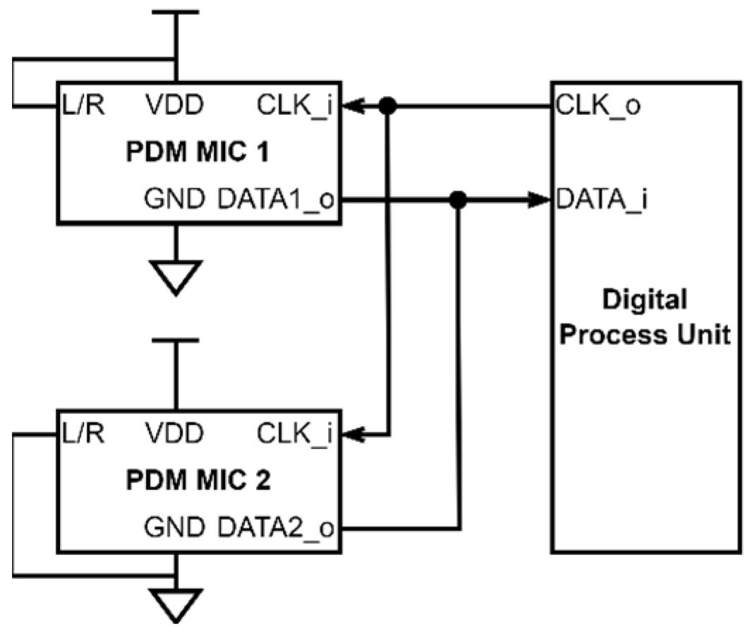
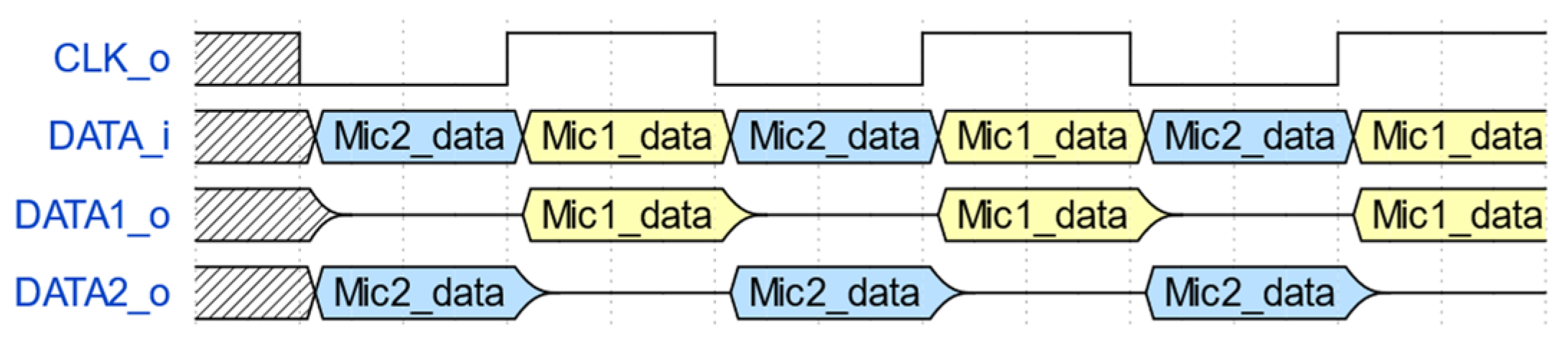
Pulse Density Modulation (PDM) microphones are MEMS devices with a simple digital interface where information is given using a one-bit digital signal. They require only two wires: one for the clock signal and another for the data signal [1]. Usually, on one PDM interface, two microphones can exist at the same time (Figure 1), because one can be set to give data on the rising edge of the clock and the other one on the falling edge of the clock, like in Figure 2.

PDM microphones use a delta-sigma analog-to-digital conversion to generate a one-bit PDM signal [2]. The information is stored in the pulse density of the signal, which has a relatively high frequency (usually 1–5 MHz).

One major advantage of the delta-sigma modulation method is its inherent noise-shaping capability. This technique pushes the quantization noise to higher frequencies, well beyond the bandwidth of the original signal. As a result, the in-band signal maintains a higher signal-to-noise ratio (SNR), while the out-of-band noise can be effectively attenuated using digital low-pass filters or anti-aliasing filters. This property is particularly beneficial in audio applications, where preserving the fidelity of low-frequency components is critical. Furthermore, the oversampling nature of delta-sigma conversion allows for simpler analog front-end circuitry, as much of the signal conditioning and noise suppression is handled in the digital domain. This makes delta-sigma-based PDM microphones not only efficient in terms of hardware complexity but also highly suitable for integration into modern digital signal processing pipelines.

An example of this type of microphone is IM72D128V01. This is a high-performance microphone manufactured by Infineon (Neubiberg, Germany), which features a Signal-to-Noise Ratio (SNR) of 72 dB(A), a dynamic range (DR) of 106 dB, and an Acoustic Overload Point (AOP) at 128 dBSPL, making it suitable for high-fidelity audio capture.

The dynamic range of a microphone can be calculated using (1) [3], taking into account that the reference sound pressure level (${SPL}_{ref}$) is 94 dBSPL [1].

$$DR=AOP-{SPL}_{ref}+SNR$$

(1)

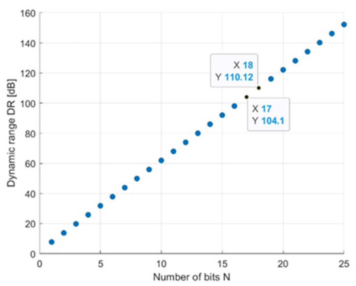
To process the information from the microphone, one needs to convert the PDM data into pulse code modulation (PCM) on a certain number of bits. The number of necessary bits depends on the dynamic range and can be determined using (2) [3], where N represents the number of bits. For the IM72D128V01 microphone, 18 bits are necessary (Figure 3).

$$DR=1.76+(N\times 6.02)$$

(2)

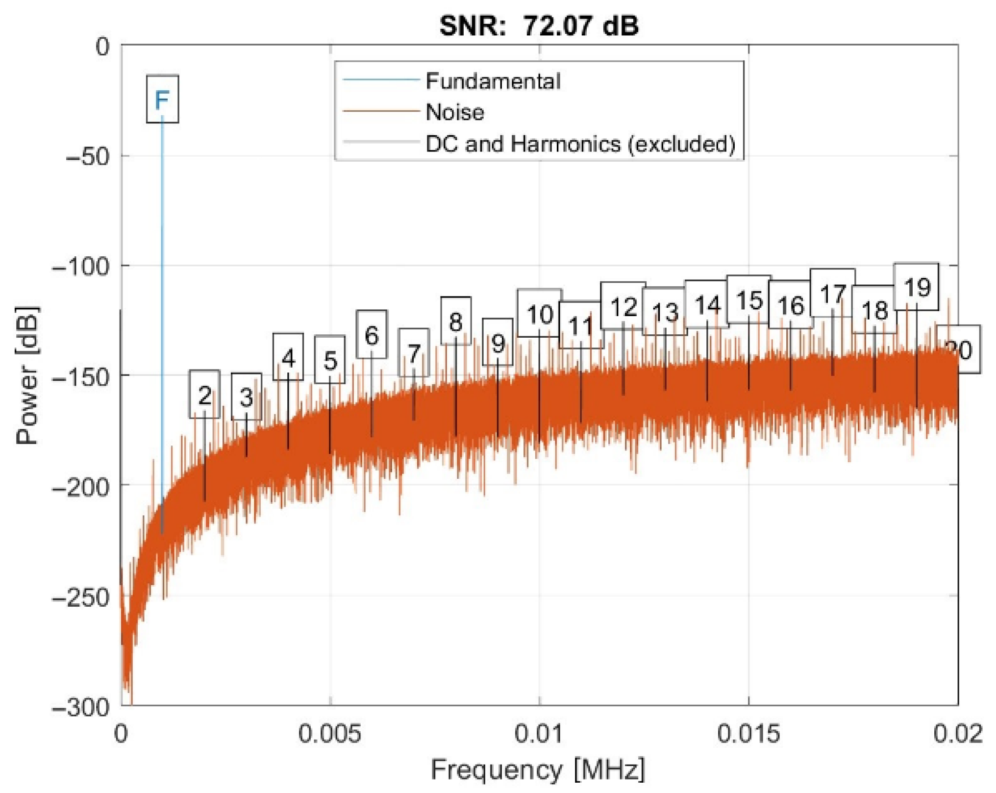
The SNR of 72 dB for the IM72D128V01 microphone is specified for a working clock frequency of 3.072 MHz and on a 20 Hz to 20 kHz A-Weighted bandwidth. To test the aliasing effect of the filters, a PDM signal (Figure 4) was generated with the ‘Delta Sigma Toolbox’ [4] in MATLAB. This signal emulates the output of the IM72D128V01 microphone using a delta sigma converter of order 3. The signal contains a 1 kHz sine wave and has approximately the same SNR on a 20 Hz to 20 kHz A-Weighted bandwidth.

To convert the PDM signal to PCM, a low-pass filter is needed to increase the number of bits per sample and then to decimate the samples to decrease the sample rate [5]. The role of the low-pass filter is to attenuate the high-frequency components to avoid the aliasing phenomenon during the decimation process.

The most suitable type of filter for PDM microphone applications is a Cascaded Integrator Comb (CIC) decimator filter. These use minimal resources because their structure does not contain any multipliers; it contains only delay registers and adders. The transfer function of the system is described by (3). The frequency response is determined only by three integer parameters, resulting in a limited range of characteristics [5]. In our case, we will analyze the CIC decimator filter with $M$ (differential delay) = 1, which will further reduce the range of characteristics. 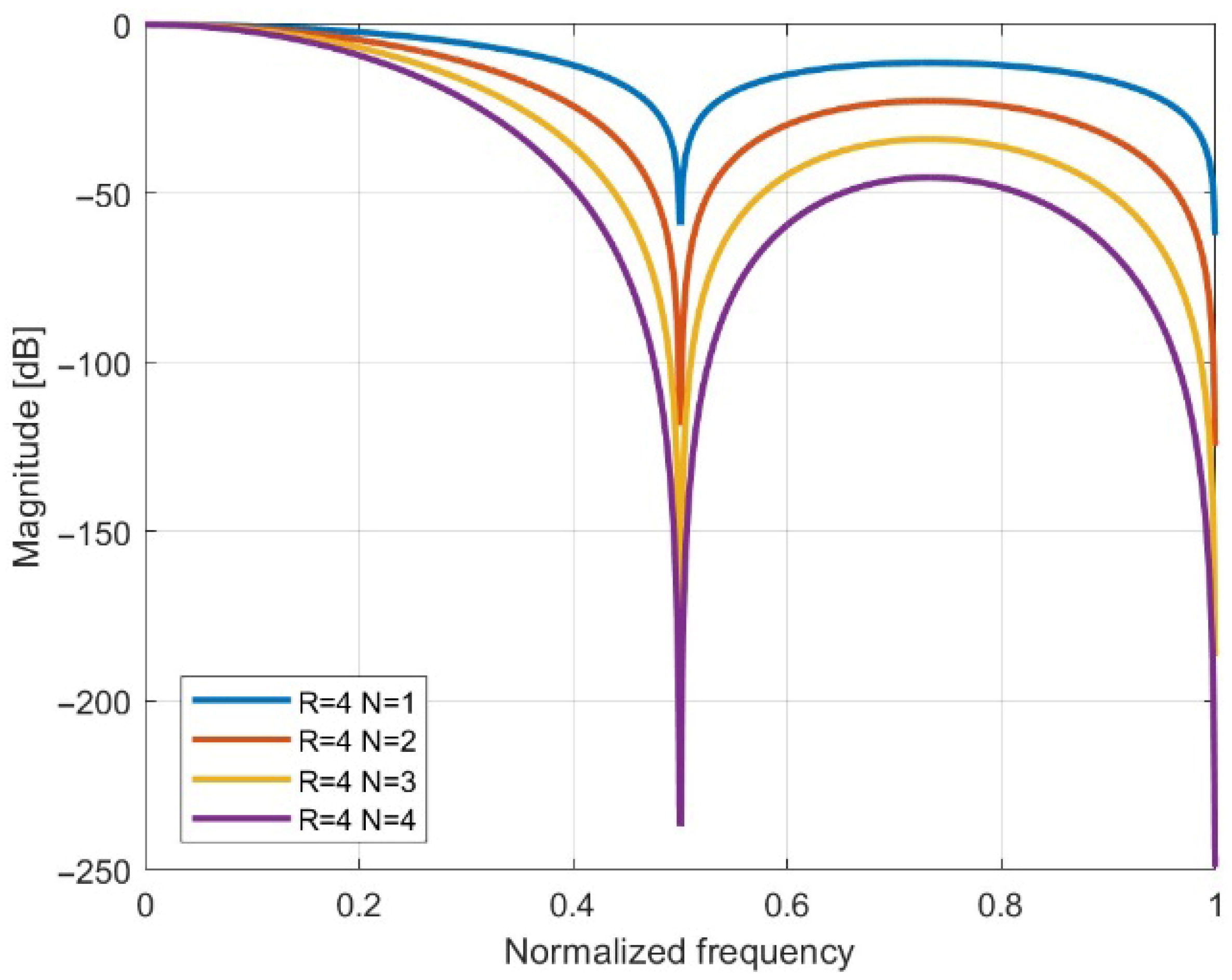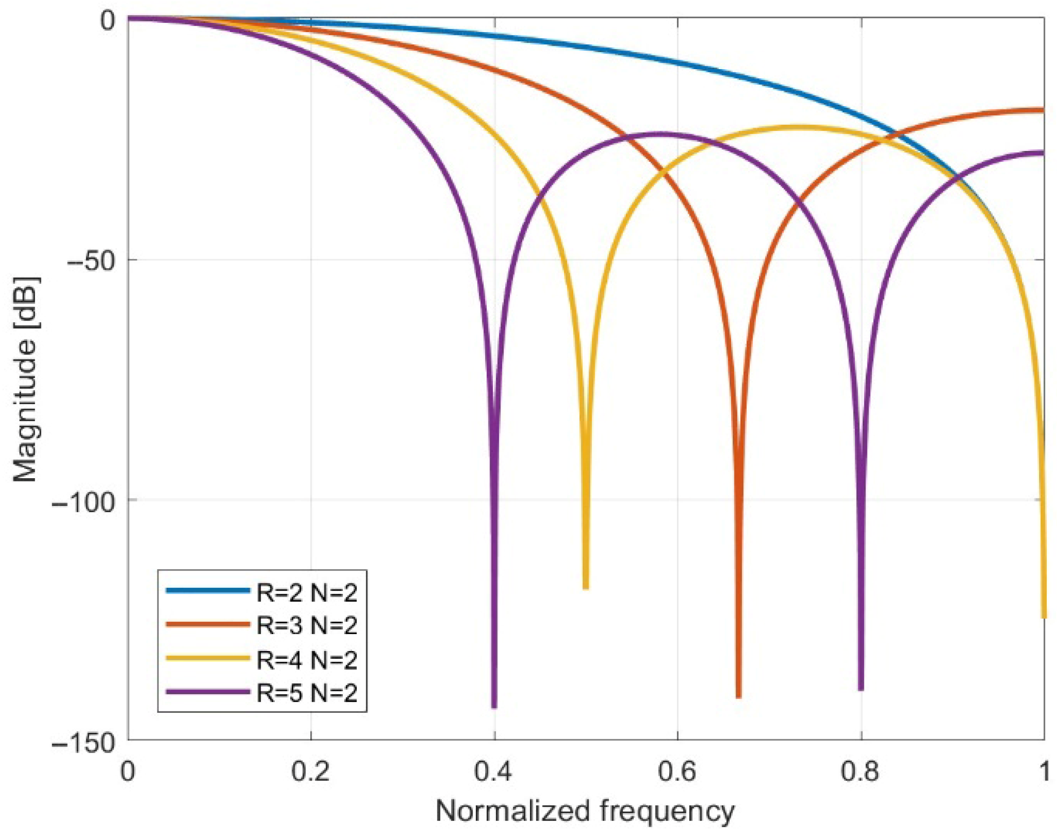The effects of varying the $R$ (decimation factor or rate change factor) and $N$ (filter order or number of stages) on the filter characteristics are shown in Figure 5 and Figure 6.

$$H\left(z\right)={\displaystyle \frac{{\left(1-z^{-RM}\right)}^N}{{\left(1-z^{-1}\right)}^N}}$$

(3)

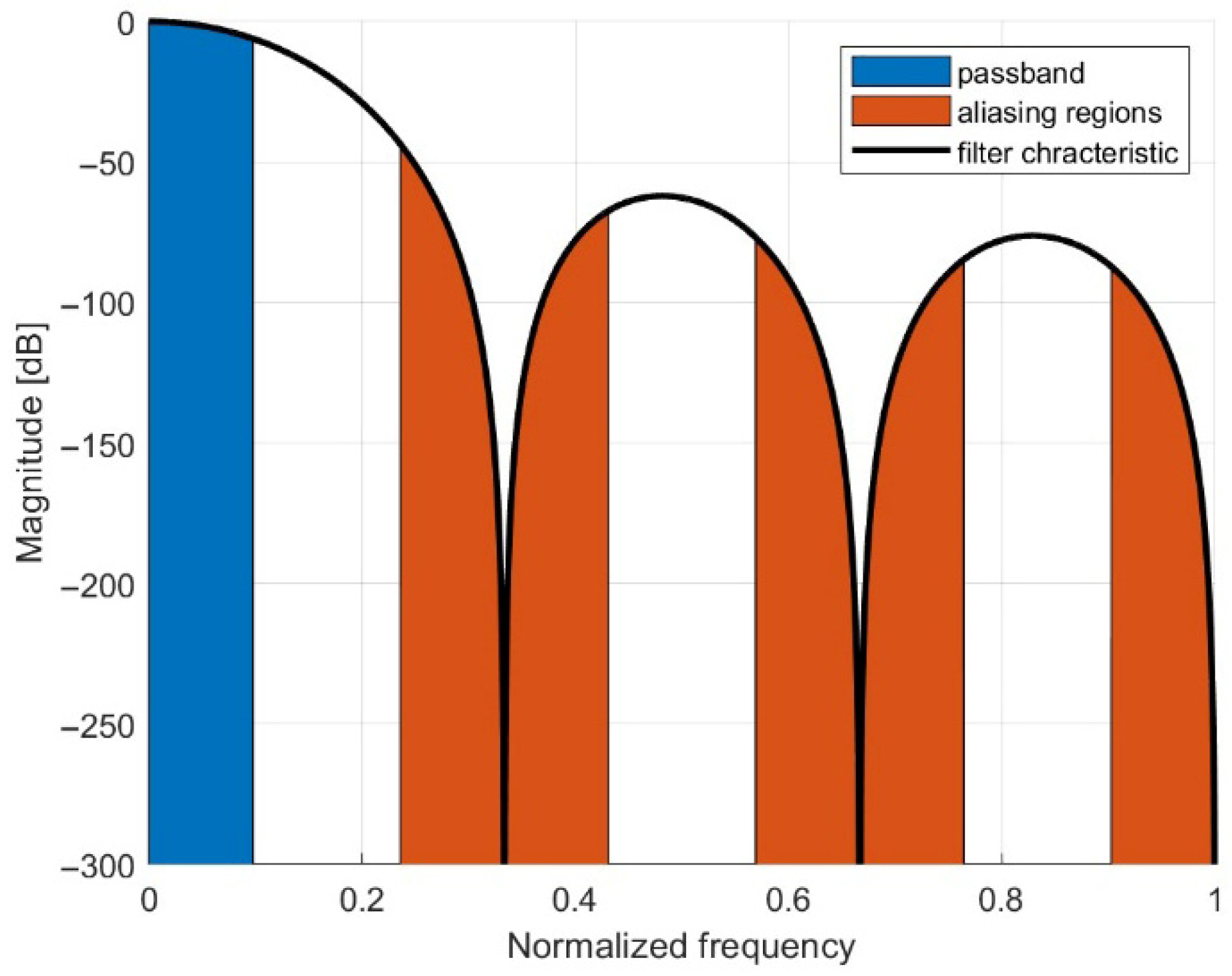
When choosing the rate change factor and the filter order, one needs to consider the aliasing effect. If the passband is $f_c$, then for every zero in the filter characteristic, we will have regions with the same width as $f_c$, which will alias into the passband, causing SNR to decrease. In Figure 7, the passband and the aliasing regions for a CIC filter with $M=1$, $R=6$ and $N=5$ are represented.

The CIC filter response in the passband is not flat; that is why a finite impulse response (FIR) filter is usually used after the filter for compensation. Several studies propose FPGA implementations of CIC compensators to mitigate passband droop. For instance, Jovanovic Dolecek and Martinez Novelo present an FPGA implementation and report absolute power and resource summaries for the compensator block, while noting a higher adder count; however, they do not quantify the incremental FPGA overhead relative to an uncompensated CIC filter [6]. In this work, we focus solely on the uncompensated variant.

While standard CIC filters represent the classical approach to decimation, recent research has explored alternative paradigms, such as data-driven conversion methods. For instance, Vitolo et al. [7] introduced a novel PDM-to-PCM conversion technique using a 1D-Convolutional Neural Network (1D-CNN) targeting ultra-low-power Keyword Spotting applications. Although such methods offer promising results for specific tasks, classical CIC architectures generally remain superior in terms of deterministic frequency response and signal fidelity for general-purpose audio acquisition. Furthermore, the utility of CIC filters extends well beyond audio processing. In the field of high-frequency instrumentation, Ming et al. [8] implemented a parallel feedforward CIC structure to achieve 20 GSPS throughput for spectrum analysis in mixed-domain oscilloscopes. Similarly, Sri Rama et al. [9] demonstrated the efficacy of VLSI-based CIC architectures for radar signal processing.

Previous research has explored FPGA-based CIC implementations for high-speed applications. For instance, Mehra and Arora [10] designed a fully pipelined CIC decimator for wireless systems using Xilinx AccelDSP, a tool that converted MATLAB algorithms into synthesizable HDL and integrated with Xilinx ISE for implementation. At that time, AccelDSP was widely adopted for DSP design automation; however, it has since been discontinued and replaced by modern workflows such as MathWorks HDL Coder, which directly generates VHDL/Verilog from MATLAB or Simulink. Previous research, such as the study by Shanthi et al. [11], has successfully utilized this workflow to implement efficient CIC filters for audio applications. In this work, we use MathWorks HDL Coder for HDL generation.

Bhakthavatchalu et al. [12] and Sachin and Ullas [13] had a similar interest, investigating different implementations of CIC filters and their required FPGA resources, but their scope was not to compare CIC filters generated with specialized tools like CIC Compiler or MATLAB. They focused on optimizing different architectures of CIC filters, and their HDL code was handwritten.

Bhakthavatchalu et al. [12] developed an implementation of a CIC filter with three stages and a decimation factor of four that used 92 slice registers and 72 LUTs, which is comparable with the results presented here.

Recent work by Datta and Dutta [14] introduced a resource-efficient CIC decimator architecture using bit-pruning and partitioned decimation factors, achieving up to 39.84% reduction in slice registers and 16.17% lower power consumption on a Virtex-5 FPGA. Unlike these architecture-level optimizations, our study focuses on comparing CIC implementations generated by different design flows under identical conditions.

CIC filters rely heavily on addition operations, so hardware optimization can also be achieved by improving the efficiency of the adders inside these filters. Recent works have proposed approximate adders to reduce power and area [15,16]. These studies focus mainly on ASIC implementations rather than FPGAs, but they highlight complementary strategies for resource optimization.

In this work, we present a post-implementation comparison of three CIC decimator design flows—AMD CIC Compiler, MathWorks HDL Coder, and an open-source RTL, reporting resource utilization and maximum operating frequency. We also introduce and validate a simplified method for estimating the maximum operating frequency of an FPGA design, demonstrating less than 10% error while preserving relative ranking. Finally, the paper provides practical insights into trade-offs between resource efficiency, configurability, and performance.

2. Results

The passband ripple for the tested CIC filter variants is presented in

Table 1. Theoretical passband ripple [dB].

		Decimation Factor
		4	8	16	32	64
Filter order	2	0.005	0.019	0.077	0.310	1.254
	3	0.007	0.029	0.116	0.465	1.881
	4	0.009	0.038	0.154	0.620	2.508
	5	0.011	0.048	0.193	0.775	3.135
	6	0.014	0.057	0.231	0.929	3.763

. These results were obtained by computing the frequency response based on Equation (3), using MATLAB.

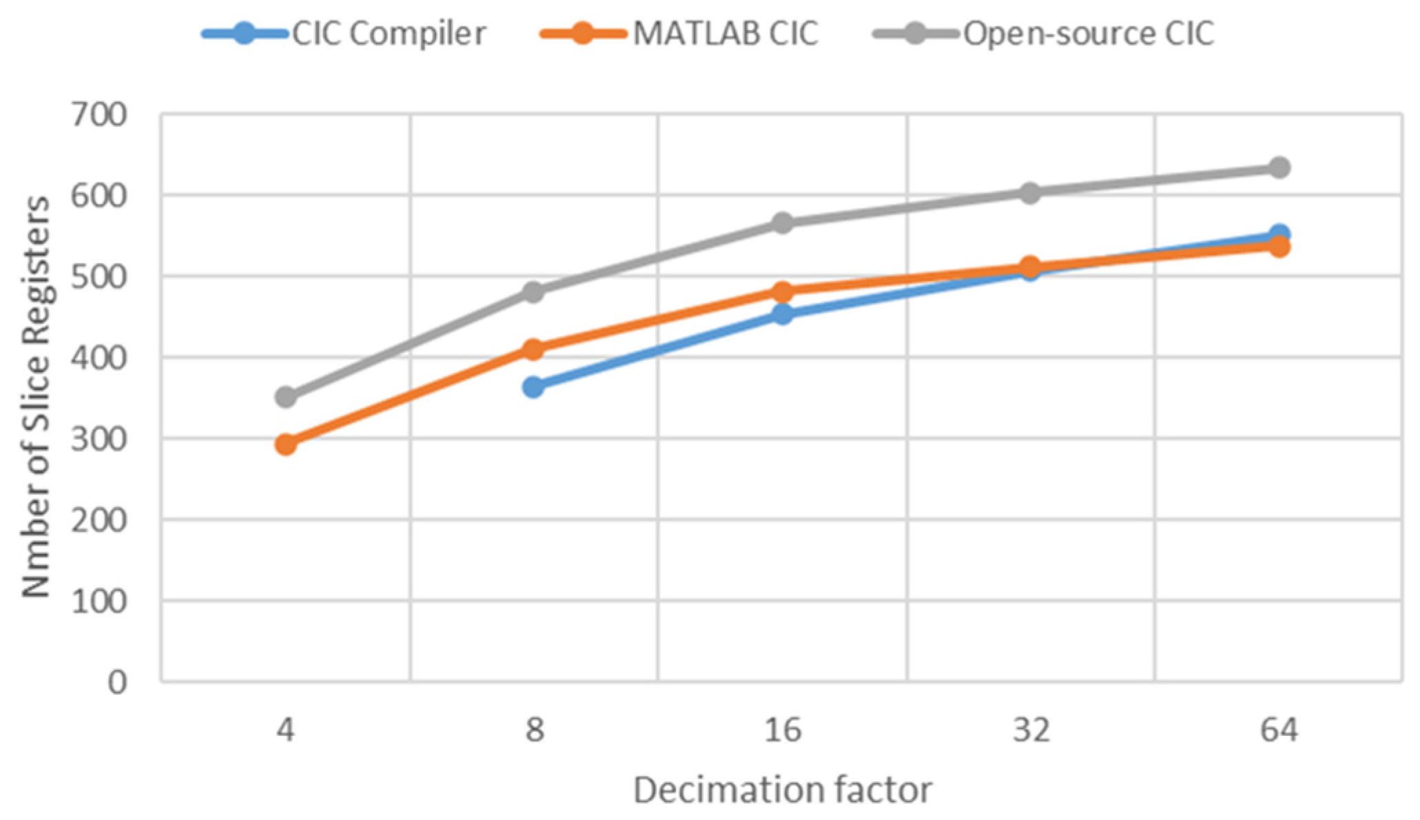
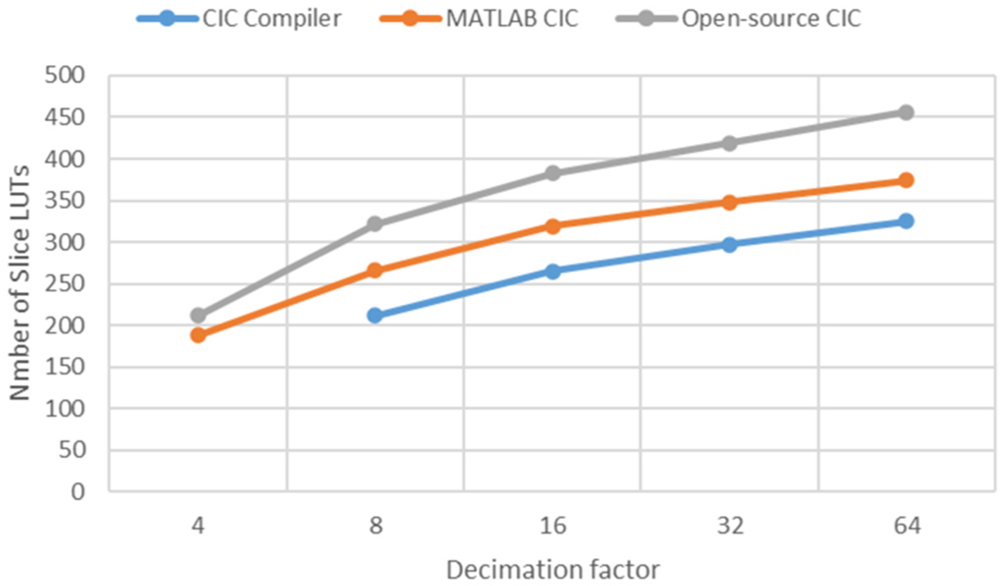
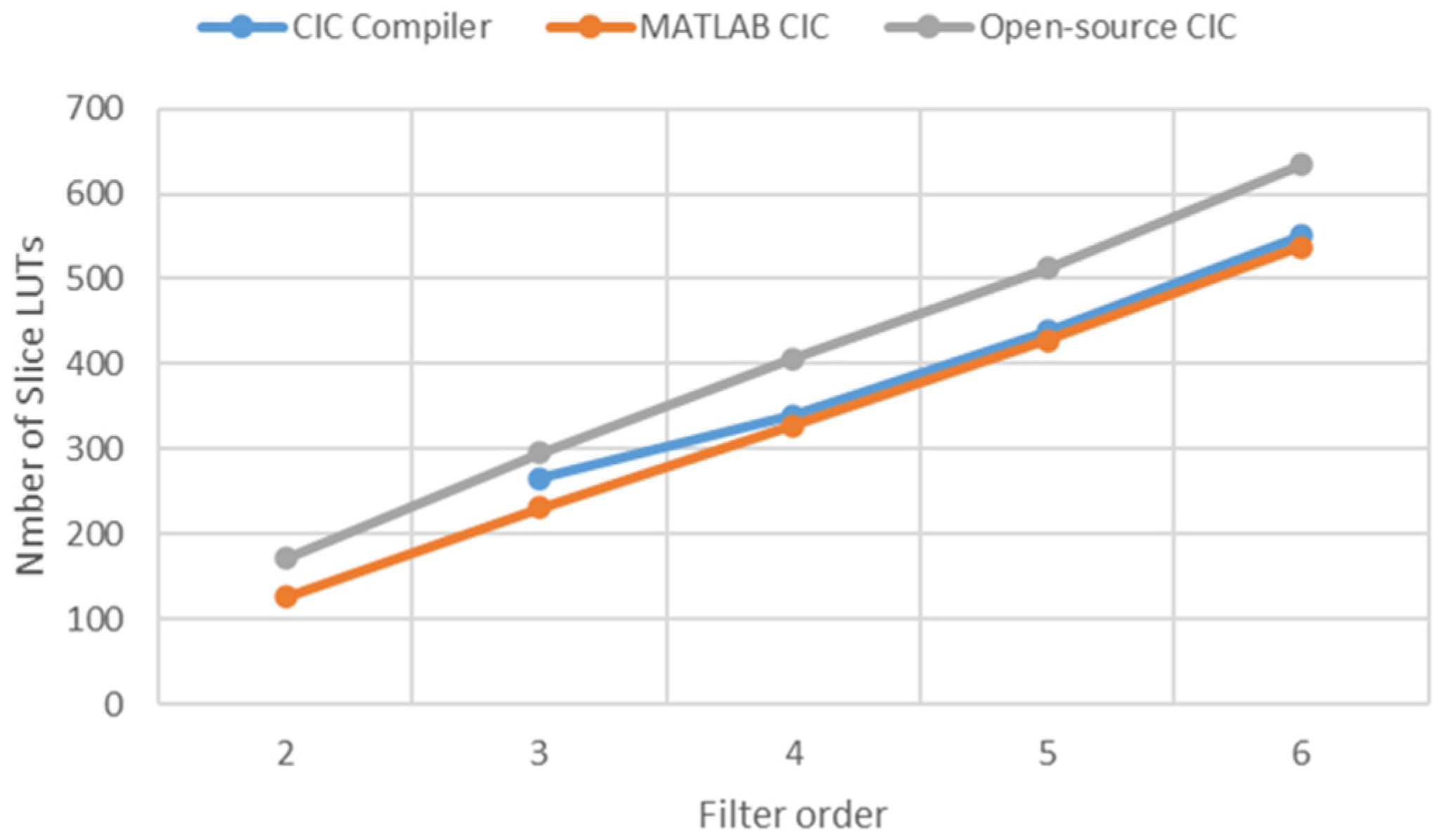
The resource utilization of the CIC filters was evaluated across three implementation platforms (Figure 8, Figure 9, Figure 10 and Figure 11).

Table 2. Slice LUTs used by CIC Compiler after implementation.

		Decimation Factor
		4	8	16	32	64
Filter order	2	-	-	-	-	-
	3	-	-	-	-	146
	4	-	-	155	188	210
	5	-	-	208	240	264
	6	-	212	265	297	325

and

Table 3. Slice registers used by CIC Compiler after implementation.

		Decimation Factor
		4	8	16	32	64
Filter order	2	-	-	-	-	-
	3	-	-	-	-	265
	4	-	-	261	307	339
	5	-	-	351	404	439
	6	-	365	453	507	551

present the results for filters generated using the Xilinx CIC Compiler, highlighting the hardware requirements specific to vendor-optimized designs. In contrast,

Table 4. Slice LUTs used by MATLAB CIC filter after implementation.

		Decimation Factor
		4	8	16	32	64
Filter order	2	34	45	56	66	78
	3	61	84	104	127	147
	4	95	132	169	198	216
	5	138	195	244	271	292
	6	188	266	319	348	374

and

Table 5. Slice registers used by MATLAB CIC filter after implementation.

		Decimation Factor
		4	8	16	32	64
Filter order	2	58	75	92	109	126
	3	99	133	167	201	231
	4	152	209	266	309	327
	5	217	303	377	408	428
	6	294	411	482	512	537

show the corresponding resource usage for filters generated using MATLAB, allowing a comparison between tool-generated implementations. Finally, the resource consumption for the open-source implementations is detailed in

Table 6. Slice LUTs used by open-source CIC filter after implementation.

		Decimation Factor
		4	8	16	32	64
Filter order	2	-	42	58	76	86
	3	60	79	108	129	179
	4	96	139	177	238	259
	5	163	232	287	319	344
	6	212	322	383	419	456

and

Table 7. Slice registers used by open-source CIC filter after implementation.

		Decimation Factor
		4	8	16	32	64
Filter order	2	-	102	125	148	171
	3	127	170	213	256	295
	4	187	260	325	381	406
	5	271	362	450	488	513
	6	351	481	566	603	634

.

The analysis of the CIC filter implementations includes several key performance aspects, such as passband ripple, maximum operating frequency, and resource utilization. The maximum operating frequencies for each filter variant, estimated using the simplified method, are presented in

Table 8. Estimated maximum frequency [MHz], CIC Compiler.

		Decimation Factor
		4	8	16	32	64
Filter order	2	-	-	-	-	-
	3	-	-	-	-	331.24
	4	-	-	315.26	307.88	315.86
	5	-	-	301.39	309.98	307.98
	6	-	322.48	307.98	299.67	304.41

,

Table 9. Estimated maximum frequency [MHz], MATLAB.

		Decimation Factor
		4	8	16	32	64
Filter order	2	410.68	405.02	406.83	366.43	327.01
	3	379.65	383.29	366.84	341.53	351.62
	4	398.88	377.79	328.08	344.47	319.90
	5	329.38	350.75	340.83	345.30	341.18
	6	334.00	344.35	333.78	318.78	310.75

and

Table 10. Estimated maximum frequency [MHz], Open-source.

		Decimation Factor
		4	8	16	32	64
Filter order	2	-	440.33	391.54	178.35	181.00
	3	414.77	386.40	284.98	252.46	114.23
	4	338.29	151.19	153.21	191.98	160.03
	5	146.43	148.54	191.17	165.29	184.91
	6	198.29	146.26	148.65	132.40	136.09

. These results highlight how different (R, N) configurations influence the achievable frequency. For comparison, the exact iterative method was also applied, and the corresponding results are summarized in

Table 11. Maximum working frequency [MHz] determined with Equation (4).

R, N	CIC Compiler	CIC MATLAB	CIC Open-Source
64, 6	308	335	145
8, 6	326	366	163
64, 3	325	379	130

, allowing a direct evaluation of the approximation error introduced by the simplified method.

As shown in Table 1, the theoretical passband ripple increases significantly with the filter order (N) and decimation factor (R), reaching over 3.7 dB for the highest configuration (N = 6, R = 64).

Table 2 illustrates the high efficiency of the vendor-optimized IP, where even the most complex configuration (R = 64, N = 6) utilizes 325 LUTs. Complementing this LUT usage, Table 3 shows that register consumption scales linearly with the filter order.

As shown in Table 4, the MATLAB-generated HDL requires approximately 15% more LUTs than the Xilinx IP. Conversely, Table 5 reveals that register utilization remains highly competitive (537 vs. 551 for N = 6).

Table 6 highlights the trade-off of the open-source implementation: while highly flexible, it consumes the highest amount of logic resources (456 LUTs at maximum complexity). Similarly, Table 7 indicates a significant increase in register usage (up to 634).

The frequency estimates presented in Table 8, Table 9 and Table 10 highlight the distinct performance characteristics of each design flow.

Finally, Table 11 confirms the validity of our simplified estimation method, showing a deviation of less than 10% compared to the rigorous iterative approach, which justifies its use for rapid comparative analysis.

To validate the functional equivalence of the three filter implementations, the emulated PDM signal described in Section 1 (Table 4), containing a 1 kHz sine wave, was processed by all three filters configured with $M=1$, $R=6,$ and $N=5$. The simulation was performed in Vivado, and the resulting PCM outputs were analyzed in MATLAB.

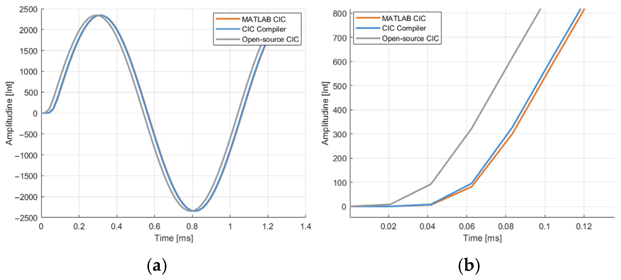
As shown in Figure 12a, all outputs exhibit the expected 1 kHz sine wave shape; however, slight time delays are observed due to differences in the internal pipeline architectures of each design. These latencies are more clearly visible in the zoomed-in view presented in Figure 12b. The measured delays between the outputs are as follows: the MATLAB CIC output is delayed by $1.95\mathrm{\mu }\mathrm{s}$ relative to the CIC Compiler output and by $22.46\mathrm{\mu }\mathrm{s}$ relative to the Open-source CIC output. Consequently, the CIC Compiler output is delayed by $20.50\mathrm{\mu }\mathrm{s}$ relative to the Open-source implementation.

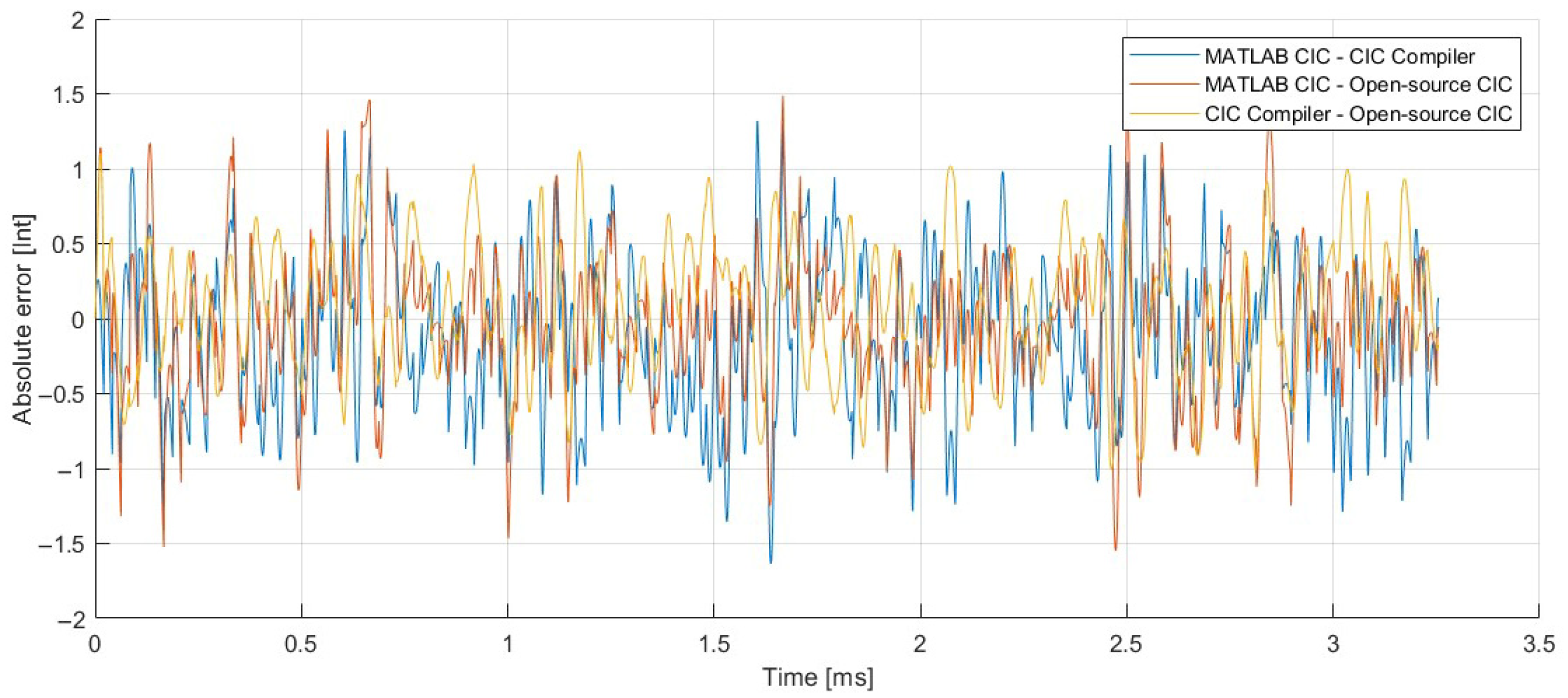
To verify signal fidelity, the waveforms were time-aligned and subtracted pairwise, as illustrated in Figure 13. The maximum absolute error observed was 1.6360. When normalized against the signal’s peak-to-peak value (approximately 4703), this corresponds to a relative error of less than 0.035%. Furthermore, relative to the full-scale range (18-bit), the error is below 0.00065%.

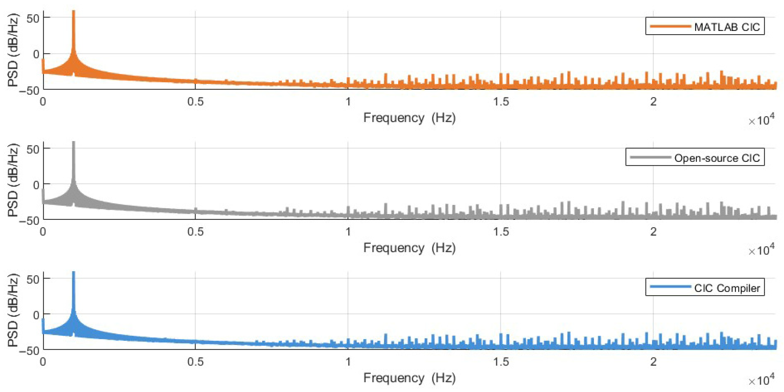
Additionally, the Power Spectral Density (PSD) was computed for each output waveform. As shown in Figure 14, the spectral characteristics are identical.

Based on these analyses, the outputs can be considered functionally equivalent, as the observed differences are negligible and likely attributable to minor quantization variations.

3. Discussion

As can be seen in Table 2, Table 3, Table 4, Table 5, Table 6 and Table 7, in most cases, the filters generated using the CIC Compiler use slightly less FPGA resources than the filters generated using MATLAB or the open-source one.

The CIC Compiler has less flexibility in choosing the filters parameters than MATLAB and open-source variant, but it has an option that can be activated, and the generated filters use DSP48 cells. These cells are FPGA resources optimized for digital signal processing. By default, CIC filters generated using the CIC Compiler utilize shift register look-up tables (SRLs) during implementation. This technique enables an efficient realization of delay elements, particularly in FPGA architectures, by leveraging the LUT-based fabric to implement long shift registers with minimal resource usage. The use of SRLs contributes to improved area efficiency and performance, especially in high-throughput designs.

The CIC Compiler also allows the generation of multi-channel filters. In this case, the architecture is better optimized because the FPGA resources are shared between the channels.

When the CIC filters are generated in MATLAB, the result is a readable Verilog code that can be edited manually if necessary. This way, we can also add the DSP48 options, but it requires more time and a good understanding of their structure.

The open-source CIC filter implementation is highly customizable and supports advanced features such as DSP48 block utilization. However, from a resource efficiency and maximum working frequency perspective, it is not as well optimized as other implementations. This trade-off between flexibility and hardware utilization should be considered when selecting a CIC filter variant for FPGA-based designs.

The highest maximum operating frequency was achieved by the CIC filters generated using MATLAB (Table 11), demonstrating the effectiveness of the HDL Coder workflow. However, the filters generated using the CIC Compiler also exhibited competitive frequency performance, confirming their suitability.

A comparative analysis was conducted to evaluate the average maximum operating frequency across the three CIC filter implementation variants. For this comparison, filters with identical parameter configurations were selected from each variant. The results showed that the CIC Compiler implementation achieved an average frequency of 311.28 MHz, the MATLAB-generated CIC filter reached 334.46 MHz, and the open-source implementation achieved 156.75 MHz. These results highlight the superior frequency performance of the MATLAB and CIC Compiler variants, while also illustrating the trade-off between flexibility and performance in the open-source implementation.

It is important to note that the maximum operating frequencies reported in this study represent near-ideal conditions. In the Vivado project, each test was conducted with only a single CIC filter instantiated at a time, and the overall resource utilization of the target FPGA remained below 1%. In practical applications, where multiple components are integrated and a significantly higher percentage of FPGA resources are utilized, timing closure becomes more challenging. As a result, the achievable maximum frequencies in real-world scenarios are expected to be lower than those reported here.

4. Materials and Methods

For analysis, we will consider a PDM microphone (IM72D128V01) which works with a $f_{clk}=3.072\mathrm{M}\mathrm{H}\mathrm{z}$ clock frequency. The human hearing frequency range is below 20 kHz, so we will consider the passband to be from 0 to 20 kHz and the stopband to be above 24 kHz (from 20 kHz to 24 kHz, a transition band is considered to occur), which will require at least a sample rate of $SR=48\mathrm{k}\mathrm{H}\mathrm{z}$. The maximum decimation factor will be $f_{clk}/SR=64$. The output is represented as mentioned before, on 18 bits. The input bit number is 2, because in our case (having a PDM input signal), the input is 1 or −1, specified in the two’s complement binary system.

Three implementations of CIC decimator filters were studied: one generated in MATLAB [17] using the HDL Coder toolbox (R2025a), one from AMD (Xilinx) (2022.2) using the Cascaded Integrator Comb (CIC) Compiler IP [18], and one using an open-source implementation [19].

A similar study was presented in [20], where FPGA resource utilization was analyzed after the synthesis stage. In contrast, the present work evaluates resource utilization after the implementation phase in Vivado, which provides a more accurate representation of actual hardware usage. This is because, during implementation, additional optimizations are performed, such as placement, routing, and logic restructuring, which can significantly impact resource consumption. Furthermore, while the study in [20] utilized a CIC filter from the dsp library, this work employs a filter from the dsphdl library. The components in the dsphdl library are specifically optimized for HDL code generation and FPGA implementation, offering improved performance and resource efficiency in hardware-centric workflows [21].

Another improvement over the methodology presented in [20] is the inclusion of a clock constraint during resource utilization analysis. In this study, the clock signal was constrained to 100 MHz, which reflects a more realistic operating condition for FPGA-based designs. It is important to note that, in certain designs, the number of utilized resources can vary depending on whether a clock constraint is applied or not. By enforcing a timing constraint, the synthesis and implementation tools may perform additional optimizations or insert timing-related structures, thereby influencing the final resource usage. This approach ensures a more accurate and consistent comparison across different CIC filter implementations.

One notable advantage of using HDL Coder is that it generates synthesizable HDL code that remains readable and modifiable, allowing for further customization or optimization if necessary. For this study, MATLAB version R2025a was used to generate the HDL code and perform related simulations.

The CIC Compiler IP version used is 4.0 (Rev 16), used together with the Vivado 2022.2 version. This IP accepts a rate change factor between 4 and 8192 (in our case, we need a maximum of 64) and a number of stages between 2 and 6. The “use DSP48 slice” option was disabled to have comparable results, because the code generated by MATLAB does not have this option.

The open-source CIC filter implementation used in this work is highly parameterizable, offering extensive customization options. Also in this case, the “use DSP48” option was disabled. For the purposes of this study, the following parameter configuration was applied:

• Input Data Width: INP_DW = 2;
• Output Data Width: OUT_DW = 18;
• Rate Data Width: RATE_DW = 32;
• Differential Delay (M): CIC_M = 1;
• Pruning: PRUNE_BITS = {(CIC_N × 2 + 2) {32’d0}} (all bits on 0 which means no pruning);
• Variable Rate: VAR_RATE = 0 (set to 0, which means decimation rate R is fixed);
• DSP Blocks: USE_DSP = 0 (set to 0, which means no use of DSP in FPGA).

The most important settings of the Vivado project where the CIC filters were synthesized are the following:

• Project device: Arty A7-100 (xc7a100tcsg324-1);
• Target language: Verilog;
• Synthesis strategy: Vivado Synthesis Default 2022 with -max_dsp option set on 0;
• Implementation strategy: Vivado Implementation Default 2022.

To determine the maximum achievable operating frequency ($f_{max}$) of a digital design targeting a specific FPGA, AMD recommends an iterative timing closure methodology, as described in their technical documentation UG949 [22]. This approach involves progressively tightening the target clock period and re-running both synthesis and implementation flows until setup timing violations occur, indicated by a worst negative slack (WNS) of less than zero. The maximum frequency is then estimated using Equation (4), where $T_i$ denotes the target clock period and $WN{S}_i$ represents the worst negative slack for implementation run $i$. Notably, the $f_{max}$ value is not directly reported by standard timing analysis tools and must be derived manually. This methodology offers a practical and reproducible means of estimating the upper frequency bound of a design under nominal and worst-case operating conditions.

$$f_{max}\left(MHz\right)=\max \left({\displaystyle \frac{1000}{T_i-WN{S}_i}}\right)$$

(4)

Considering that, in this case, the design consists solely of a CIC filter, the methodology described above was simplified. Instead of employing an iterative process, the clock frequency was directly constrained to a fixed frequency, based on the assumption that the implemented CIC filter variants can reliably meet timing at this frequency without violations. The maximum frequency ($f_{max}$) was then calculated using Equation (5). To validate this simplification, a series of tests was conducted to compare the results of the original iterative method with those obtained using the simplified approach.

$$f_{max}\left(MHz\right)={\displaystyle \frac{1000}{T-WNS}}$$

(5)

For most CIC filter implementations, the simplified method was used to estimate the maximum achievable frequency. The iterative method was applied to all three CIC filter variants with the following $(R,N)$ pair: $\left(64,6\right),\left(8,6\right),\left(64,3\right).$ These pairs were selected to represent extreme cases within the scope of this study: $(R_{max},N_{max})$, $(R_{min},N_{max})$, and $(R_{max},N_{min})$, where $R_{max}$, $R_{min}$, $N_{max}$, and $N_{min}$ denote the maximum and minimum values of the decimation factor (R) and the number of stages (N) used in the tested filters. The results were compared with the simplified method, and the error was under 10%, demonstrating that the simplified method provides a sufficiently accurate estimation of the maximum achievable frequency for practical purposes. Moreover, the simplified method is computationally faster, which is particularly beneficial when comparing multiple filter variants. Since all filters were evaluated using the same simplified approach, the relative comparison between them remains valid and relevant.

The value of $T$ used in Equation (5) was determined based on results from the original iterative method and was adapted according to the specific CIC filter variant. For filters generated using MATLAB, a clock period of $T=3.333\mathrm{n}\mathrm{s}$ was used. In the case of the CIC Compiler variant, $T=3.448\mathrm{n}\mathrm{s}$ was applied, while for the open-source implementation $T=10\mathrm{n}\mathrm{s}$ was selected. These values also ensured that all implementations within each specific variant did not exhibit negative worst slack, thereby confirming that the selected clock periods were within the feasible timing margins for each design. For instance, enforcing a tight constraint of $T=3.333\mathrm{n}\mathrm{s}$ on the open-source variant would result in excessive timing violations, rendering the analysis invalid. Conversely, applying a more relaxed constraint $T=10\mathrm{n}\mathrm{s}$ to the other two variants would prevent the implementation tool from fully optimizing the critical paths, leading to an underestimated $f_{max}$.

5. Conclusions

This work presented a post-implementation evaluation of three CIC decimator filter design flows for FPGA: AMD CIC Compiler, MathWorks HDL Coder, and an open-source RTL implementation. The study compared resource utilization and maximum operating frequency under identical conditions and validated a simplified method for estimating $f_{max}$ with less than 10% error.

The results indicate that CIC Compiler achieves the lowest resource utilization and provides multi-channel support, making it ideal for area-constrained FPGA designs, while MATLAB HDL Coder delivers the highest maximum operating frequency; in contrast, the open-source implementation offers extensive configurability but sacrifices efficiency, requiring more resources and delivering lower frequency performance.