Low-Overhead Reinforcement Learning-Based Power Management Using 2QoSM ^†

Abstract

With the computational systems of even embedded devices becoming ever more powerful, there is a need for more effective and pro-active methods of dynamic power management. The work presented in this paper demonstrates the effectiveness of a reinforcement-learning based dynamic power manager placed in a software framework. This combination of Q-learning for determining policy and the software abstractions provide many of the benefits of co-design, namely, good performance, responsiveness and application guidance, with the flexibility of easily changing policies or platforms. The Q-learning based Quality of Service Manager (2QoSM) is implemented on an autonomous robot built on a complex, powerful embedded single-board computer (SBC) and a high-resolution path-planning algorithm. We find that the 2QoSM reduces power consumption up to 42% compared to the Linux on-demand governor and 10.2% over a state-of-the-art situation aware governor. Moreover, the performance as measured by path error is improved by up to 6.1%, all while saving power.

1. Introduction

From Internet-of-Things devices to data centers, computing systems remain power constrained. These constraints are found in thermal limits, battery capacity, economic cost or the physical delivery of power. Power management means different things depending on the context, but fundamentally, computers control power consumption by reducing the performance of system devices. Effective power management lies in finding which devices and power settings reduce power without significantly degrading performance.

In CPUs, dynamic power management is centered around dynamic voltage and frequency scaling (DVFS) [1] and power gating [2,3]; DRAM may reduce refresh rates [4,5] and hard drives may power off [6]. The use of these techniques often reduce performance, but if a device is underutilized or idle, this trade-off is worth making. This situation becomes significantly more complex when we look at modern systems. The real-time requirements, low-latency interactivity, or mixed or changing boundedness can make simple power management policies less effective or tenable. The emergence of heterogeneous computational units (e.g., big.LITTLE) and memory (DRAM + NVM) as well as peripherals with large power budgets (e.g., accelerators) only increase the complexity of power management optimizations.

The solution presented in this paper aims to confront this complexity through greater cooperation between the software and hardware. Avoiding the difficulty of hardware–software co-design by using a software framework allows us to use application guidance and performance data and hardware state information to make effective proactive power-management decisions. These policies are undertaken by a Q-learning-based quality-of-service manager (2QoSM).

Section 2 places this work into the state of the art, identifying improvements over existing systems as well as work that is complementary. Section 3 expands on the motivations for this system. Section 4 details the software architecture including an overview of Q-Learning and the implementation of the Q-Learner Quality of Service Manager (2QoSM). Section 5 demonstrates the effectiveness of 2QoSM on an autonomous robot. Section 6 discusses the lessons learned from this research and the future directions of our work.

2. Related Work

Power consumed by a computing system can be described by the equation

$$P_{sys}=P_{CPU}+P_{mem}+P_{disk}+P_{net}+P_{per}$$

(1)

where the system power $P_{sys}$ consists of the sum of the power consumed by the CPU (including co-processors) $P_{CPU}$, memory system $P_{mem}$, storage $P_{disk}$, networking $P_{net}$ and other peripherals $P_{per}$. The contribution of components in Equation (1) vary significantly between computing systems. Early PC requirements looked much different from what we see today. A standard computer in the mid-1990s could have the monitor consuming well over half of its total power budget, 20% from the large, spinning hard disk, and less than a watt used by both CPU and memory together [6]. By comparison, modern CPUs can consume significantly more power, anywhere from less than 5 W for a notebook processor to 400 W for a large server processor (5-800x) [7]. Enterprise and HPC systems can spend up 40% of total power budget on DRAM alone [8] In mobile devices, the OLED/LCD display may consume 25% [9], 50% [10] or more [11] of the energy budget. While a phone’s radios may consume power equal to the display, in embedded IoT devices this makes up the majority [12]. It is clear that the power consumed by various subsystems in different systems varies dramatically and requires complex power management schemes.

The first techniques of power management involved simply turning off the system during idle periods, initially manually. Early automated power management determined when a system was idle and powered down components using a standard interface such as Advanced Power Managment (APM) [13] and Advanced Configuration and Power Interface (ACPI) [14].

2.1. Dynamic Voltage and Frequency Scaling

Arguably the most important technological advance in computer power management was dynamic voltage and frequency scaling (DVFS). Its effectiveness is clear when we examine the power consumed by a CPU, expressed [15] by the equation

$$P_{CPU}=p_t(C_L\ast V\ast V_{dd}\ast f_{clk})+I_{sc}\ast V_{dd}+I_{leak}\ast V_{dd}$$

(2)

where $p_t$ is the probability of transition (activity), $C_L$ is capacitive loading, V is logic voltage, $V_{dd}$ is supply voltage, $f_{clk}$ is clock frequency, and $I_{sc}$ and $I_{leak}$ are short-circuit and leakage currents, respectively. The capacitive loading of the circuit $C_L$ [16] and leakage current $I_{leak}$ [17] are a fact of the underlying digital design. The use of power gating [2,3] can reduce the leakage current; however, this requires hardware enabling and, when available, can be controlled by the same types of mechanisms as DVFS. The short-circuit current $I_{sc}$ is caused by transitions and thus directly related to clock frequency, but because it is based upon transistor design it can be treated as a constant consumption [18]. Activity $p_t$ as a power-management technique is improved through software efficiency, but fundamentally the instructions executed are represented by transitions and thus cannot be dynamically controlled without changing the underlying software.

This leaves voltage and frequency as the primary control variables of dynamic power management allowing Equation (2) to be simplified [1] as:

$$P_{CPU}\propto V^2·f$$

(3)

where the CPU power consumption $P_{CPU}$ is directly proportional to the voltage V squared times the clock frequency f.

For a power manager to operate, there are two fundamental requirements: (1) knowledge of the computing system’s state and (2) the ability to change the power state of a device. In the simple case of software running on a CPU, power management was relatively simple: adjust the DVFS states (known in ACPI as P-States) to reduce the processor idle time. The situation becomes more complex when there are heterogeneous processing units and power consumption is dependent on which cores are executing the process. When we expand our management from CPUs and other heterogeneous computational units to memory, networking, and peripherals, normal optimizations become infeasible because changes in any given subsystem may have dependencies to other systems. For example, slowing memory devices may increase latency and thus stalls in the CPU pipeline, reducing the efficiency of the CPU power management. Similarly, spinning down a disk prematurely and forcing it to power up before accessing data can cause significant wasted power by the CPU while waiting.

The most common and straightforward method of using DVFS is to target a desired system load (say, 65%) and step up or down the P-states to reach it. This is the policy used by the default Linux on-demand governor: it measures the idle time of the CPU and increases or decreases the CPU P-State in order to reach its target [19,20]. There are more sophisticated strategies for controlling DVFS including periodic workload scheduling [21], integrated run-time systems such as CPU MISER [22], CoScale [23], or energy quota-based systems like Intel’s RAPL [24].

An alternative paradigm of power-management is known as race-to-idle [25,26] or race-to-halt [27]. This is possible because modern processors are able to quickly power down regions of the CPU (power-gating). Instead of trying to optimize the voltage states, we use the highest possible performance state to complete the work and immediately attempt to power down. Using DVFS states, especially when attempting race-to-halt, relies on the assumption that the task is compute bound as opposed to memory bound. A computationally bound process is only limited by the speed of instructions retired by the CPU and will directly benefit from increasing a processor’s frequency (and thus retirement rate). However, if the process is memory bound, increasing the CPU performance will not significantly speed up execution [28] while still using more power. Thus, other techniques must be used such as memory frequency scaling [29], offlining memory pages [30], reducing refresh rates [31], and the use of heterogeneous memory [32,33]. Mixed workloads are more of a challenge because they may benefit from DVFS periodically as the program changes execution regions. Li et al.’s work on COS shows how one could model the expected performance from different power states using a combination of offline and online profiling in scientific applications described as mixed workloads [34]. An advantage to using a machine-learning informed policy is that if race-to-halt turns out to be the best policy for a given combination of workload ans system, the policy will converge to that, while still being flexible enough for more memory-bound or mixed workloads. This work also attempts to optimize the power consumption and performance mixed workloads by modern techniques for power management as described below.

2.2. Modern Power Managers

As computer systems become more powerful both in the sense of computational performance and literal power consumption, there is a greater opportunity to use extra CPU cycles for more efficient predictive power management and scheduling. Many of these systems are described in the literature as “power managers” or “power and performance managers” but we will refer to them more generally as “quality-of-service managers” (QoSM) or QoS management. This more generalized term encompasses the broad spectrum of hardware and software targets, constraints and goals. The two primary areas that are related to our work are middleware for quality-of-service management and machine learning-based power managers.

The use of middleware, a software abstraction layer between application and operating system, for power and performance management has been examined by researchers for more than two decades. Li et al. introduced a performance-aware middleware for distributed video systems in an attempt to balance the objectives of hardware and application [35]. Shortly after, Zhang et al. developed ControlWare, a system for QoS management in distributed real-time systems and propose the idea of convergence guarantees that lie between hard and probabilistic performance guarantees [36]. This use of feedback-control theory to manage resources based upon an application’s QoS is closely related to our system in concept but differs in target application and scope. ControlWare is intended for distributed systems and makes use of coordination entities that are not useful for a single-purpose system.

Hoffman et al. demonstrate the danger of trying to optimize for accuracy and power without coordination and propose CoAdapt, a runtime controller for dynamic coordination of performance, accuracy and power [37]. We believe the attempt to balance accuracy (error) and power consumption by adjusting both hardware and application algorithm is an effective strategy and we make us of this idea in our work. Where the systems diverge is in target application/hardware (embedded v. enterprise) and choice of QoSM (feedback control v. machine learning). In the past couple years, systems power management using control theory have been proposed including those based upon SISO [38] and a supervisory and control theory (SCT) [39]. We agree that the formalism of control theory has its place in power management; however, we believe the very stability and rigor that are obtained by control theory can limit the optimizations available when interactions between systems become more complex.

Other recent examples of using a software framework, specifically using big.LITTLE-based platforms, are the work done by Muthukaruppan et al. which use hierarchical controllers [40] and price-theory [41]. Where their framework is evaluated using computationally intensive benchmarks, our work is focused on complex physical system controllers which we believe are more challenging to optimize and thus require more complex techniques. Similarly, a software framework for resource management in control systems was developed on a big.LITTLE platform [42]. This work did not attempt voltage and frequency control, but did take into account the available resources when starting and stopping controllers.

Imes et al. developed a series of hardware- and software-agnostic frameworks for power management in real-time systems. POET, a C-based framework, minimizes energy consumption while still meeting soft real-time constraints of a set benchmarks [43]. They then expanded upon POET to create Bard which allows for runtime switching between power and performance constraints [44]. POET/Bard are closely related not only due to their framework architecture but also their use of the ODROID-XU3 as an experimental platform. Bard uses a set of frequencies and their associated speedups and power usages that must be computed offline, whereas our learner simply has knobs to turn and dials to read. Therefore, 2QoSM provides an advantage for memory-intensive or mixed workloads when the calculated speedup associated with a specific P-state is an optimistic upper bound for a compute-bound workload.

The 2QoSM described in this work was designed as a drop-in replacement for a situation-aware governor [45]. We make use of the framework and experimental platform to demonstrate both the ease of replacing the power manager, as well as the improvements of the Q-learner over a simple governor. Additional differentiation between the two frameworks is described in more detail in Section 4.

2.3. Machine Learning in Power Management

There have been numerous recent machine learning-based power managers. Of these, a large number have used reinforcement learning to identify a policy for a given state of a CPU [46]. We frame dynamic power management as a reinforcement learning problem in more detail in Section 4.2.

Martinez and Ipek [47] evaluate machine learning as a tool for making low-level power management decisions such as DRAM scheduling and allocation. In a CPU + FPGA + DSP heterogeneous computing system running image processing applications, Yang et al. manage power consumption using a regression-based learner [48].

A number of researchers have used Q-learning specifically to develop policies for power management. Ye and Xu attempt to reduce power consumption with a Q-learning by optimize idle periods [49]. Our 2QoSM in that Ye and Xu attempt to reduce the number of state transitions, while 2QoSM is only concerned with the measured error and power consumption. If frequent transitions are increasing power consumption through leakage current, because we are measuring the real-time current, we believe 2QoSM should identify this and adjust the policy accordingly. In addition, ref. [49] was done in simulation using synthetic benchmarks while the experimental platform in this work is an application running on real hardware.

Shen et al. select DVFS states using a Q-learner by constraining performance and temperature while attempting to minimize the total energy [50]. The metrics used are CPU intensiveness (similar to stall–cycle ratio [28]), instructions-per-second and temperature. Even though they make similar design decisions as those we discuss in this paper, our work has some notable differences. Most importantly, our reward and state are not based upon CPU utilization (i.e., IPS) but instead the measured application performance, which in the case of a physical system is much more representative of total system performance than CPU load. In addition, because their constraints are given by the user, scenarios can arise in which the learner cannot find a policy that meets the desired constraints.

Ge et al. also use CPU metrics, user-identified constraints and temperature for determining state and reward [51] Das et al. allocate threads and set DVFS states using a Q-learner to to obtain a desired performance target [52]. Their work is centered on thermal limits, especially as they relate to temperature-dependent leakage current and mean-time-to-failure (MTTF). Time-based deadlines are their performance targets, while because our application’s execution time is not known a priori, we must use runtime metrics to determine application performance. Gupta et al. use deep Q-Learning (DQL) using a similar big.LITTLE SBC to obtain near-optimal performance per watt [53]. We agree with the authors that DQL is a viable dynamic power management strategy, it does have significant drawbacks that our work does not. DQL requires the creation of an Oracle, requiring a significant amount of offline training and benchmarking. For a non-deterministic physical system, may not only be a significant amount of work but actually impossible.

3. Motivation

As discussed in Section 2, there are many different techniques of software-controlled power management. In one extreme, you have generic one-size-fits-all techniques in general purpose operating systems such as Linux’s on-demand governor. These techniques work across a variety of systems and tend to work well in overall, but due to their generality, remain greatly suboptimal. At the other extreme, there is strict co-design, wherein policies and applications are designed for a specific hardware platform and have direct control over all settings. Careful co-design allows the possibility of strong correctness guarantees and near-optimal performance/power consumption, but tight coupling requires significant engineering work and eliminates cross-platform portability. With the huge number of individual platforms, especially among single-board computers (SBCs) and systems-on-a-chip (SoCs), this tight coupling is a serious drawback.

An ideal system would have the benefits of co-design, namely, interaction between application and hardware but without the tight integration that makes portability difficult. Our work attempts to create such a system by allowing application state, performance, and guidance as well as hardware state and control to be abstracted and managed through a power controller. This controller does not have to understand the specifics of provided state or available actions, only that its actions result in state changes. From the observed state changes, it can determine via a reward function, which actions provide the best outcomes in a given state.

Moreover, by providing a communications channel between application and hardware, we no longer have to rely on simple computational metrics of performance, but instead can use both quantitative and qualitative application and whole-system performance. For example, when running the blacksholes benchmark [54], the result obtained from a given dataset is the same across all platforms, only the execution time differs. However, in a phyical system, we are focused not only on the speed of execution but the quality of execution, because the targeted algorithms are non-deterministic either due to the presence of a physical plant or because the algorithms themselves have multiple possible outcomes (e.g., quality settings of video encoding).

4. System Overview

Our system consists of two primary components: the middleware and the power-manager itself. The motivation and design of the middleware architecture is discussed in Section 4.1 with a particular emphasis on aspects that differ from previous work. The power manager itself, the 2QoSM, is discussed in Section 4.2, beginning with its place in machine learning-based power managers, followed by details of implementation.

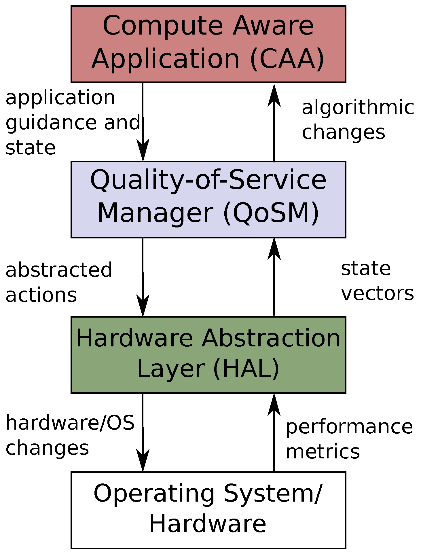
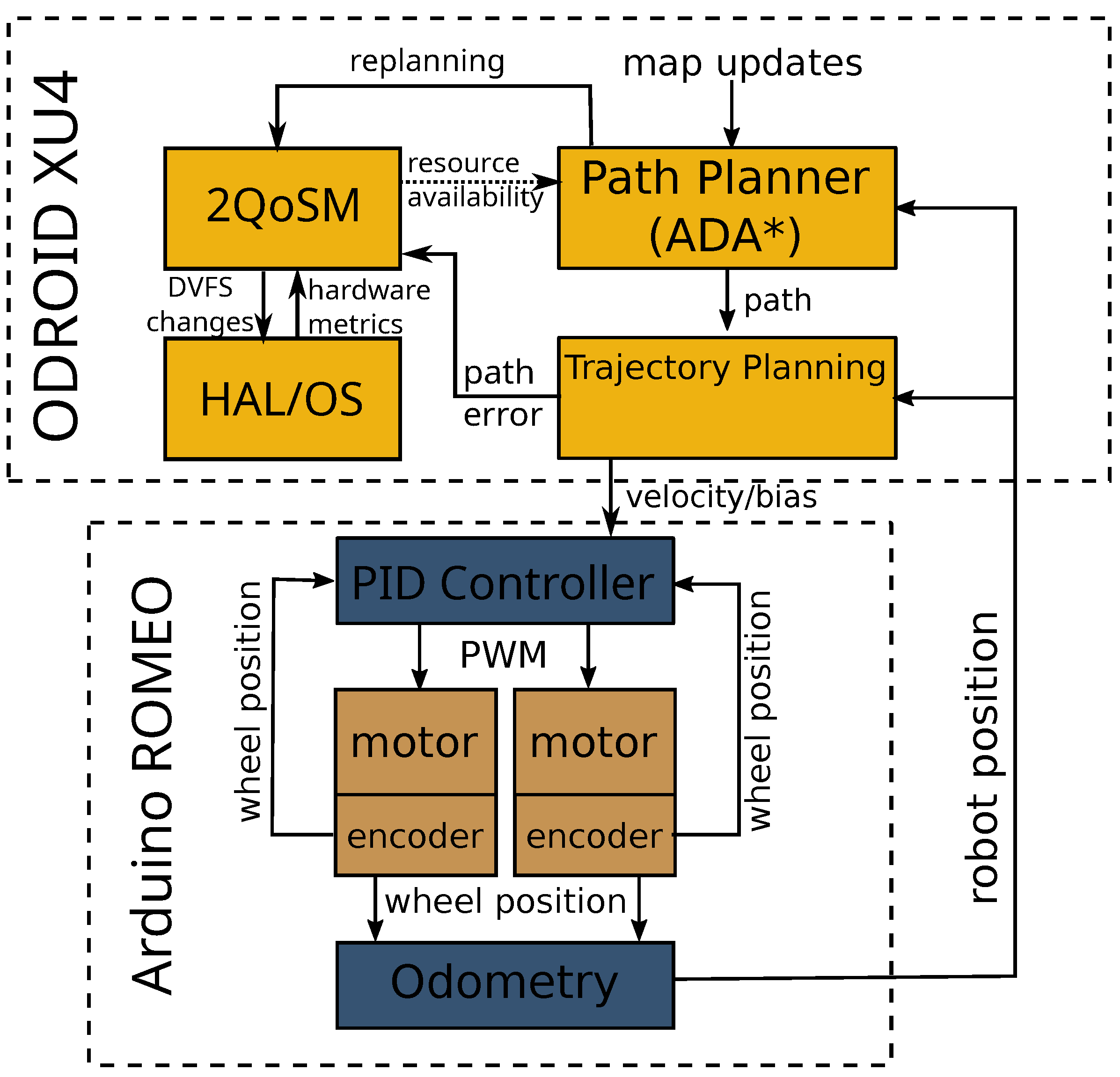
4.1. Software Architecture

The primary goals of the underlying software architecture are modularity and reusability. One of the reasons why standard power management techniques have been unchanged for so long (e.g., Linux’s on-demand governor) is because, aside from working well enough, they do not require tightly coupled integration with the underlying hardware. Specifics of hardware control are abstracted through drivers and the /sys virtual filesystem. While this allows for easier programming and some measure of universality, it prevents a predictive and intelligent power manager from using all the information and configuration at its disposal.

To meet the goals of abstraction and controllability, we use the layered architecture shown in Figure 1. It consists of three primary components: compute-aware applications, hardware abstraction layer and a quality of service manager. As discussed in Section 2, the middleware is based upon the work presented in [45] and differs primarily in abstraction level, discussed below.

We define compute-aware applications (CAAs) as programs which meet two needs of controllability, namely, the ability to change algorithms dynamically and to provide a progress or performance metric. CAAs can be composed with their individual controls and outputs shared with the QoSM. The CAA state is continuously monitored by the QoSM. This state consists of both metrics (e.g., latency, error) and application guidance to the hardware. Most importantly, the QoSM does not have to understand the meaning of a specific metric or guidance is, it is only required to integrate it into a state vector or feature reduced state. While we do not attempt feature reduction in this work, it has been effective for modeling and prediction in GPUs [55] and CPUs [56]. The QoSM takes this state vector and uses a policy—or set of policies—to take an action. Again, this action does not have to be understood by the QoSM, it is only required to observe the outcome. As an analogy, the QoSM turns an unlabeled knob, and then observes the reward obtained from its action. The actions are then converted by a hardware abstraction layer (HAL) into low-level platform-specific hardware or operating system changes.

In the other direction, the operating system sends metrics such as hardware performance counters, CPU load, memory utilization, slack time, temperature, or power measurements to the HAL. The metrics end up in a (possibly featured reduced) state vector which is passed to the QoSM. Much like the QoSM sends actions to the HAL, the QoSM may also suggest algorithmic changes to a CAA. For example, if the QoSM finds there is excess capacity in the system, it can advise a CAA to use higher performance algorithms (e.g., processing higher resolution frames or conducting deeper searches). Alternatively, when the QoSM believes capacity is limited, it can notify CAAs, allowing applications to choose to degrade more gracefully. By coordinating the behavior or application and hardware, more intelligent and tailored power management policies may be developed.

4.2. Q-Learner Quality of Service Manager (2QoSM)

As other researchers have demonstrated and as discussed in Section 3, reinforcement learning is a good choice for managing DVFS states and algorithmic profiles of applications. Q-leaning is a specific technique for reinforcement learning which works absent any underlying model [57]. Without a model, Q-Learning estimates a real-valued function Q of states and actions where $Q(s,a)$ is the expected discounted sum of future rewards for performing action a in state s [58]. Q-values are saved in a $s\times a$ Q-matrix. We calculate Q using the function

$$Q_{new}(s_t,a_t)=(1-\alpha )·Q(s,a)+\alpha ·(r_t+\gamma ·\underset{a}{max}Q(s_{t+1},a_t))$$

(4)

where $Q_{new}(s_t,a_t)$ is the new value at time tin the Q-matrix at $(s_t,a_t)$. $\alpha$ is a learning rate, $r_t$ is the instantaneous reward at time t, $\gamma$ is the discount factor, and ${max}_{a}Q(s_{t+1},a_t)$ is an estimate of an optimal future value. The learning rate $\alpha \in [0,1]$ is used to balance new information with previously calculated Q values. As $\alpha \to 1$, Q updates are more affected by new rewards, whereas a smaller $\alpha$ gives more importance to existing Q values. The discount factor $\gamma$ weighs future versus present rewards. In other words, if the discount factor is large, future rewards are preferred, while a small discount factor favors immediate rewards. $\gamma =0$ creates an algorithm that maximizes only instantaneous rewards, while $\gamma \ge 1$ does not converge and Q values will become infinite. To determine the optimal future value, the learner determines the best possible Q available based upon action a.

Algorithm 1 shows the algorithm used for updating the Q-matrix. To initialize the learner, an $S\times A$ Q-matrix is allocated where S is the number of states and A is the number of actions. Though are implementation initializes the Q-matrix values to zero, it is possible to randomly initialize the matrix [59] or to pre-populate the Q-matrix for faster convergence [60]. At the beginning of every step, the learner observes current state $s_t$. After examining the values in row $Q\left(s_t\right)$ it takes, based upon its selection policy, an action—most often the action with the highest $q_{s_t,a}$. During training instead of taking the best action, it is good practice to take a random action with probability $\rho$ to better explore the action–reward space. It is also possible to lower learning rate $\alpha$ as the Q-learner converges, preventing outliers from overly affecting a well-trained learner. After the action is taken, the learner observes the reward r and $Q_{new}(s_t,a_t)$ is updated using Equation (4).

Algorithm 1 Q-Learning Update

1: if t = 0 then 2:    Initialize Q-matrix $\forall a,s,Q(s,a)=0$ 3: end if 4: while  $s_{t+1}\ne endstate$  do 5:    Determine current state $s_t$ 6:    Find ${max}_{a}Q(s_t,a)$ 7:    Take action a based on policy 8:    Calculate instantaneous reward r 9:    Update Q based upon Equation (4) 10: end while

As the system moves traverses states by taking actions, successive updates to a previously encountered $Q(s,a)$ begin to decrease in magnitude, thus the learner converges. In infinite time Q-learners converge to an optimal policy, however the parameters of $\gamma$, $\alpha$ and $\rho$ can lead to very different learners in finite time [61].

Most problems approached with Q-learning have a fixed end state. Once this state is reached, the algorithm ends, and a new epoch begins, reusing the existing Q-matrix. However, it is also possible to use Q-learning for non-episodic tasks i.e., those without a terminal state. As long as the system finds itself in previously encountered states, the learner can still improve its its Q-function. This non-episodic (and potentially indeterminate) model is well-suited for power management.

5. Experimental Results

There are three reasons why an autonomous robot was selected to test the 2QoSM. First, due to being battery powered, an autonomous robot has a limited power budget, and a reduction in CPU energy consumption means more power for the motors, and thus a longer run time. Furthermore, the power consumption is relatively balanced between two components: the ODROID XU4 and the motors. Thus, a less-optimal path may use less CPU energy, but the path may require significant more energy for the motors due to starting and stopping or large numbers of sharp turns. Second, path and trajectory planning have a mixed performance profile, consisting of regions of both computationally and memory intensive execution. The path planning algorithm is also anytime, meaning the more computational effort spent finding a path, the better the path obtained. Third, the application has a very important metric of overall system performance: physical system error measured as deviation from the ideal path.

Section 5.1 details the test platform, Section 5.2 describes the software implementation of 2QoSM, Section 5.3 examines the training and convergence of different reward functions, and Section 5.4 and Section 5.5 evaluate the overall performance of the system.

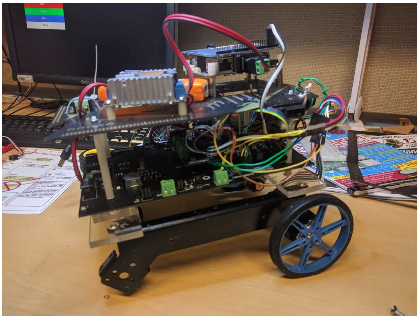
5.1. Experimental Platform

The autonomous robot is based upon the DF Robot Cherokey 4WD [62]; however, it has been significantly modified. The robot can be seen in Figure 2. Aside from physical modifications, the computational system has been split, creating a custom, stacked heterogeneous architecture, consisting of two separate computational units: an Arduino ROMEO BLE ATMega328/P [63] and an ODROID XU4 [64].

A block diagram of this architecture is shown as Figure 3. The Arduino ROMEO BLE is adept at the low-level operation of the motors via built-in H-Bridge motor controllers. In addition, the ROMEO has analog and digital general purpose input-output (GPIO) pins for sampling and operating sensors. The basic motor control is done via PID control. In addition, it uses sensor data to make odometry calculations and transmits needed data via SPI to the ODROID XU4. It runs PID motor controllers, makes odometry calculations and is connected via SPI to the upper-level ODROID XU4.

This data is used by the ODROID XU4 for mapping, route planning and trajectory planning. The ODROID XU4 is build around a Samsung Exynos5422, an ARM big.LITTLE processor. The XU3 and XU4 are very similar and have been used extensively as a test platform in previous research into intelligent power management [39,43,44,45,53,65]. The ARM big.LITTLE heterogeneous multiprocessing architecture (HMP) consists of two clusters of cores: four high performance, higher-power Cortex-A15 cores and four lower-performance, lower-power Cortex-A7 cores. DVFS operates on a per-cluster granularity [66] and threads are scheduled automatically between the two types of cores [67]. The default scheduler is used in this research; however, using the 2QoSM to schedule threads on cores (as an available action) is possible in future research. It runs a stock version of Ubuntu Linux 18.04 with kernel v4.14.5-92. The details of the platform are summarized in

Table 1. Platform Overview.

high-level controller	board	ODROID XU4 [64]
	processor	Samsung Exynos5422 8-core big.LITTLE [68]
	DRAM	2 GB
	storage	16 GB eMMC
	network	802.11b wireless via USB
	operating system	Ubuntu 18.04
	kernel	Linux 4.14.5-92
low-level controller	board	Arduino ROMEO [63]
	processor	ATMega 328P

.

The robot acts in a 12 m × 12 m course, divided by the mapping algorithm into 1,440,000 1 cm squares. There are three walls in the environment that force the robot to slalom in order to make it to the end point. For path planning, the robot uses Anytime Dynamic A* [69], which is well suited for use as a CAA because the path quality is iteratively and monotonically improved the longer the algorithm executes. If there exists a path through the obstacles, ADA* is guaranteed to find a correct path using a single iteration. However, with more resources (i.e., execution time), it can find more efficient paths, eventually searching the entire search space and finding an optimal path. If the robot detects a new obstacle, it updates the location in the map, and notifies the planning thread, which recalculates the path. The trajectory planner (also in its own thread), uses the information obtained by the odometry and determines the necessary maneuvers to follow the calculated path. These commands are passed to the ROMEO via SPI.

5.2. Quality-of-Service Manager Implementation

The 2QoSM was written as a drop-in replacement for the situation-aware governor [45]. Rather than using an existing Q-learning library (e.g., pytorch [70]), we implemented the Q-Learner in C using the GNU Scientific Library (GSL) [71]. While an existing library has advantages, there were a few motivating reasons to implement our learner from scratch. First of all, the majority of machine learning libraries are written in Python, a language generally unsuited for performance-critical systems programming. Second, while there are C++-based machine learning libraries, this would require moving from an entirely C-based architecture. Fortunately, Q-Learning is a fairly simple algorithm and was easily implemented using only the GSL.

In line with the multi-threaded controller architecture, the Q-Learner runs in its own thread, with a 10 ms sample period. Timing is handled using Linux high-resolution timers (hrtimers) Upon activation, the conditional at line 4 of Algorthm 1 is tested, and if the robot is not in its end state, it begins its update.

First, the QoSM collects available metrics, discretizes them and packs them to states. We assessed several different state vector compositions, but the data we present in this paper use the state variables shown in

Table 2. State Vector Composition.

Metric	Discretization Levels	Cumulative States	Size (B)
error	10	10	400 B
power consumption	10	100	4000 B
replanning mode	2	200	8000 B
checksum error	4	400	16,000 B
map updates	2	1600	64,000 B

. As the third column shows, as we increase the number of discrete levels of the state variables, the increase in state space size is multiplicative. The entries of the Q-matrix are represented by a 64 bit (8 B) double and there is one value per action, per row. Though each individual row in the Q-matrix is only 40 B, the multiplicative increase in matrix size makes the selection of state variables and the discretization precision very important. However, even with 1600 states, the Q-matrix is only 64 KB large. A simple optimization would be to replace the 64 b double with a 32 b float, either halving the size of the matrix or allowing for twice the number of states.

Once the learner determines its current state, it finds the row in its Q-table that is associated with this state. Based upon the current policy, it selects the best action. The policy used in this work is, with probability $\rho =0.9$, to choose the action with the highest future reward, otherwise take a random action. After taking the action, the learner calculates its reward function as a result of the action taken, and updates $Q(s_t,a_t)$. The timer is then reset and the thread goes back to sleep for 10 ms.

The state of the robot, its power consumption and location in the test region can be observed from an ncurses-based console as shown in Figure 4. This simple but responsive interface allows monitoring via the network, allowing for remote operation with minimal computational overhead.

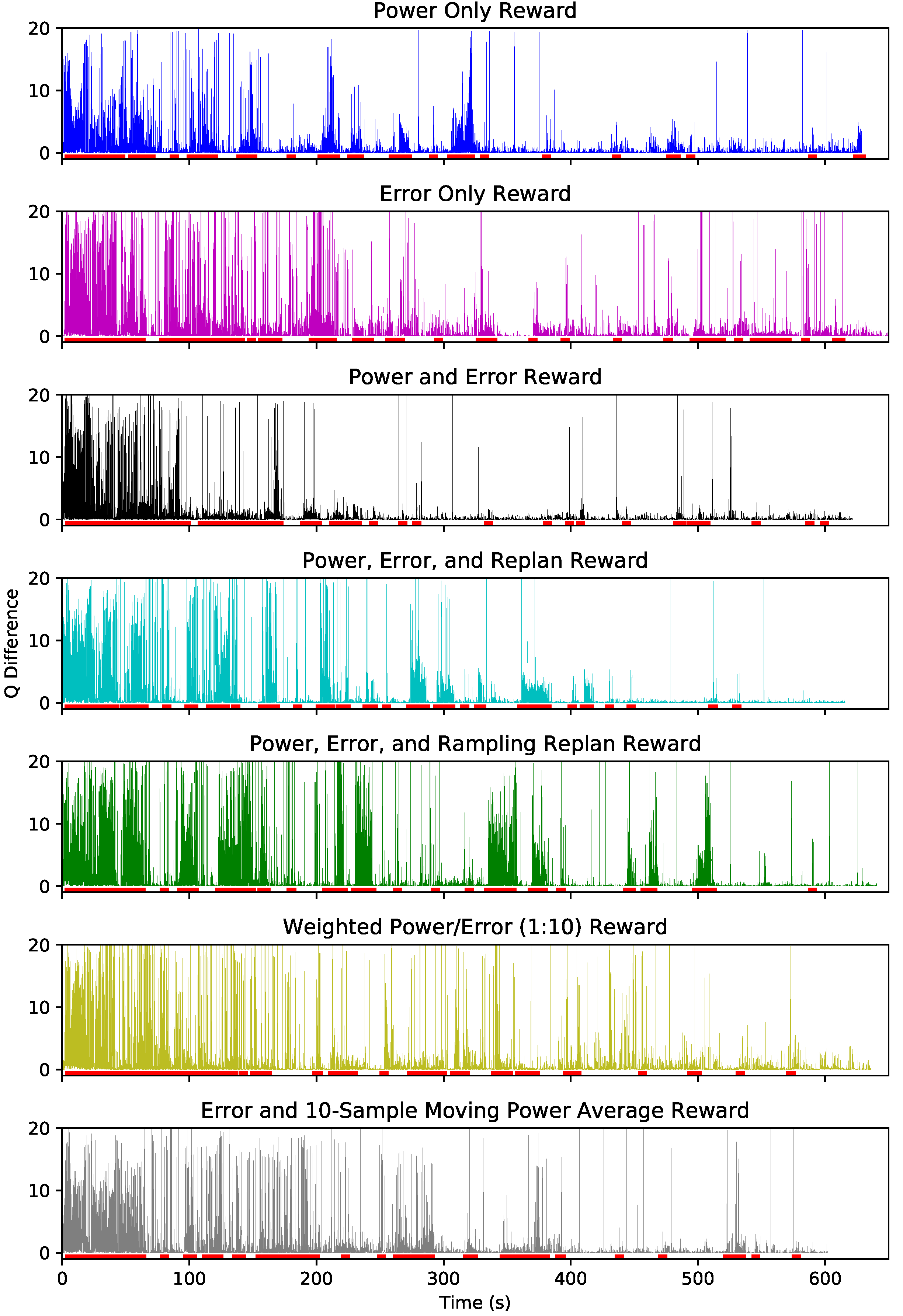
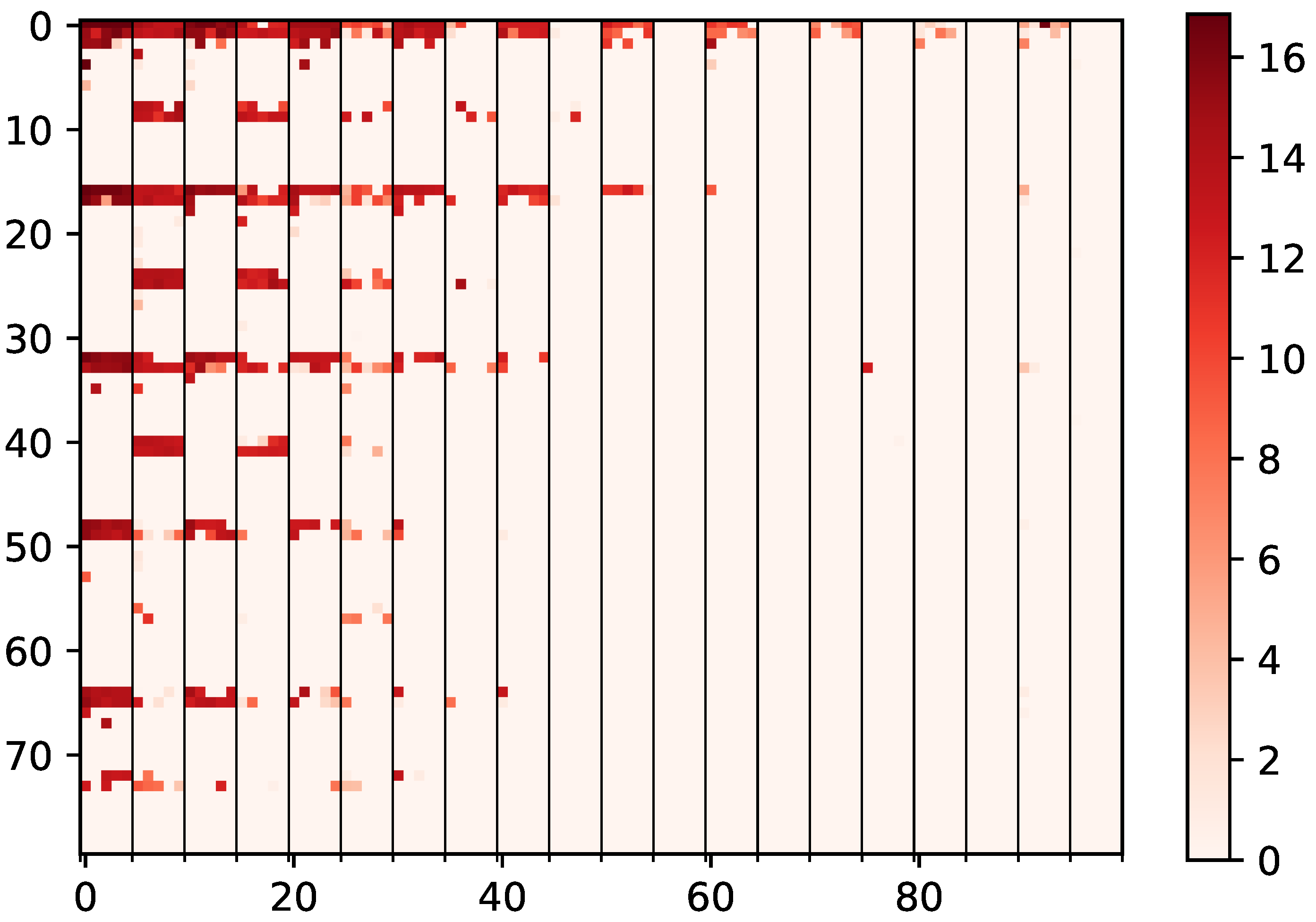
5.3. Training and Convergence

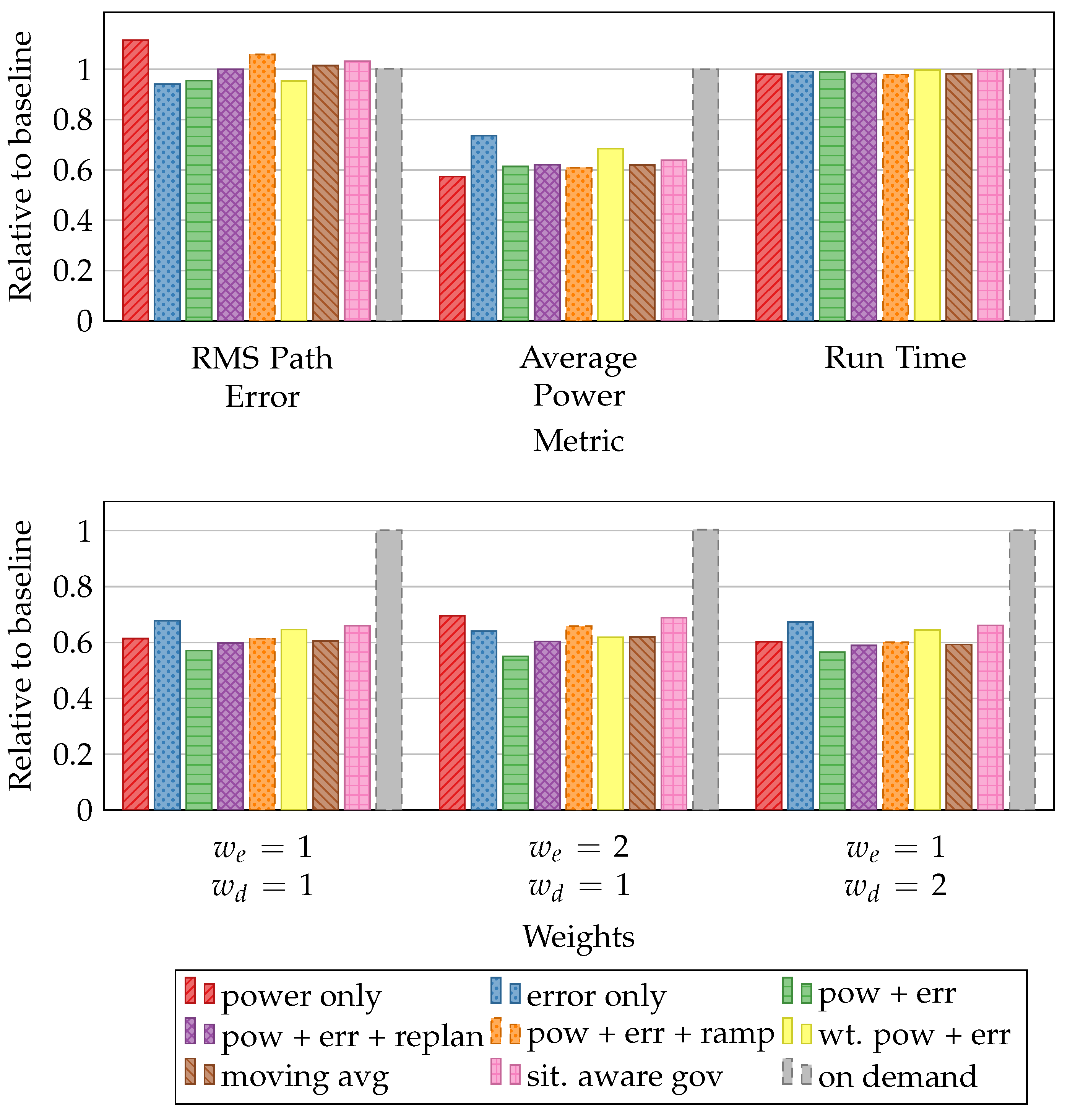
To train the Q-Learner, the robot navigated to randomly selected coordinates in an environment filled with obstacles. Figure 5 shows a sample training run. To determine adequate convergence of the learner, we observed a windowed average of the magnitude of the Q updates. When the update remained below a threshold for a certain amount of time, the algorithm was considered trained. The longest period of training was approximately 600 s, so we ran all reward functions to a full 600 s. These trained matrixes were then fixed, and used at the start of each experiment presented in Section 5. As Q-learning is an online-learning algorithm, it will continue to update its policy constantly, each successive run has a further-trained learner. Although we did not see any indication that successive runs using an increasingly trained learner gave a noticable performance improvement, for better comparison of results, the matrix obtained after the 600 s of training were reused at the start of each run.

In a production implementation of 2QoSM, a few changes could be made for greater robustness. For one, the Q-Learner could itself determine when training had reached a certain quality by observing the magnitude of Q-matrix updates. From this is could reduce the probability of a random action $\rho$ and the learning rate $\alpha$, reducing the exploration and update rate.

The variables used in the reward functions are shown in

Table 3. Symbols Used in Reward Functions.

Symbol	Description
t	Time of sample
$P_t$	Instantaneous Power at time t
$P_{max}$	Maximum measured power
$E_t$	Error measured at time t
$E_{max}$	Maximum measured error
r	ADA* replanning active (0, 1)
$\sum r$	Accumulating sum of replanning
${\overline{P}}_n$	n-Sample moving Average of Power

.

Figure 6 shows the updates to the Q-matrix at each sample time for seven different reward functions described in

Table 4. Reward Functions Tested in 2QoSM.

Number	Reward Description	Reward Function
1	Power Only	$1-{\displaystyle \frac{P_t}{P_{max}}}$
2	Error Only	$1-{\displaystyle \frac{E_t}{E_{max}}}$
3	Power + Error	$2-\left({\displaystyle \frac{P_t}{P_{max}}}+{\displaystyle \frac{E_t}{E_{max}}}\right)$
4	Power + Error + Replan Flag	$3-\left({\displaystyle \frac{P_t}{P_{max}}}+{\displaystyle \frac{E_t}{E_{max}}}+r\right)$
5	Power + Error + Accumulating Replan Flag	$3-\left({\displaystyle \frac{P_t}{P_{max}}}+{\displaystyle \frac{E_t}{E_{max}}}+\sum r\right)$
6	Weighted 1:10 power to error	$1-\left(0.1·{\displaystyle \frac{P_t}{P_{max}}}+0.9·{\displaystyle \frac{E_t}{E_{max}}}\right)$
7	Error + 10-sample Moving Average of Power	$2-\left(E_t+{\overline{P}}_{10}\right)$

. The absolute value of the update to Q-values are shown on each y-axis, and the training time is shown on the x-axis. Periods when the robot is replanning its path are indicated by red bars underneath each plot. Over the 600 s of learning the magnitudes of Q-updates decrease as the policy converges. The error-only reward function is the least convergent due to the difficult-to-predict relationship between CPU power consumption and robot path-following. We see similar difficulties in convergence when error is weighted more heavily as in the 6th reward function (weighted error/power).

On the other hand, the power-dominated reward functions converge quickly because the Q-learner easily and correctly determines that to maximize reward, simply reducing the P-state is effective. The 10-sample moving average, which adds a delay to the reward, is learned quickly thanks to the discount factor $\gamma$, adding value to time-delayed rewards.

To get a better understanding of the state space of the Q-learner, Figure 7 shows a heatmap of the Q-matrix after a completed training session. The darker the color, the greater future reward associated with a given state–action pair. Here we can see that there is obvious clustering due to the state creation and discretization. The lightest colored squares of the Q-matrix are states that were seldom or never reached or provided very little reward. The order in which the state vector is packed with the state variables determines the layout of the Q-matrix. The most significant bits of the state vector are the error term. Because the error in general remains low, the majority of the states reached are in the left side of the matrix. Further clustering occurs due to the map updates being fairly infrequent and replanning mode being the most computationally intensive section of the program, thus being correlated with higher power states. This distribution and under-utilization of the Q-matrix shows the value of more sophisticated methods of state discretization such as adaptive state segmentation [72,73]. Another option for greater utilization of the state space while reducing the matrix size is Deep Q-Learning [53]; however, this introduces challenges discussed in Section 2.3.

5.4. Metrics

The performance of each reward function is compared to the Linux on-demand governor [19] and a situation-aware governor [45]. Figure 8 compares average path error, power and navigation time across 10 runs each. As previously mentioned, the Q-learner updates the Q-matrix during the course of the run, but before starting any successive runs, it reloads the post-training Q-matrix.

These basic metrics demonstrate the behavioral differences between the various reward functions. This can be seen quite clearly when examining the power-only and error-only rewards. If the learner optimizes for power, it obtains the lowest power consumption of any governor or reward function, but also has significantly higher error. Conversely, if the learner aims to only minimize error, it has lower error than all other policies but at the cost of a higher power consumption than all but the Linux on-demand governor. As the run-time remains approximately the same for all governors, the reduction in average power correspond to total energy savings and thus total robot battery life.

The power-only reward function reduces power consumption by 2.98 W (42.6%) compared to the on-demand governor and 0.457 W (10.2%) compared to the situation-aware governor. RMS error is minimized using an error-only reward function, showing a 6.1% improvement over on-demand and 8.9% over the situation-aware governor. This is an interesting result, since previous work had shown that the on-demand error was very close to a static high-power setting. The most likely explanation is that the proactive application guidance during replanning mode proactively prepares for computationally-intensive regions better than the reactive power management of on-demand. This is because while on-demand keeps average power high because of the fairly active application (trajectory planning, communications, etc.); however, it still attempts to adjust P-states, finding itself in a less-than-optimal performance state when activity spikes. The reward function that sums power and error lowers power consumption in comparison to the Linux on-demand governor by 2.703 W (38.7%) and to the situation-aware governor by 0.18 W (4.0%). We also see an improvement in error over on-demand and situation-aware governors by 4.6% and 7.49% respectively.

When making decisions about whether to reduce performance (and execution time) in return for energy savings, it is helpful to use energy delay product (EDP) [74,75]. The EDP is

$$\mathrm{EDP}=E·T^w$$

(5)

where E is normalized energy, T is normalized task time, and w is the weight placed on performance. The on-demand governor is used as the baseline for energy and execution time. All evaluated QoSMs significantly outperform the on-demand governor, and all but the error-only and weighted power and error outperform the situation-aware governor. Because the actual traversal of the path is quite close among runs, the power-minimizing algorithms always perform the best, obscuring differences between the reward functions.

For this reason, we include the energy-error delay product (EEDP) [45]

$$\mathrm{EEDP}=E·{ϵ}^{w_e}·T^{w_d}$$

(6)

where E and T are normalized energy and runtime as in Equation (5), $ϵ$ is the normalized system error, $w_{ϵ}$ error-term weighting, and $w_d$ delay-term weighting. By including error into this metric, it is possible to evaluate different policies more clearly. We can differentiate between the performance as it relates to energy, error, and delay. These results are shown on the bottom of Figure 8. If energy and delay are given the same weights, the power-only reward function continues to outperform the others. However, if we emphasize either error or delay, the power-and-error sum reward function shows better performance. By adding EEDP as an evaluation metric for power management decisions, researchers can better select the policy that meets system goals by differentiate between the behavior of different algorithms.

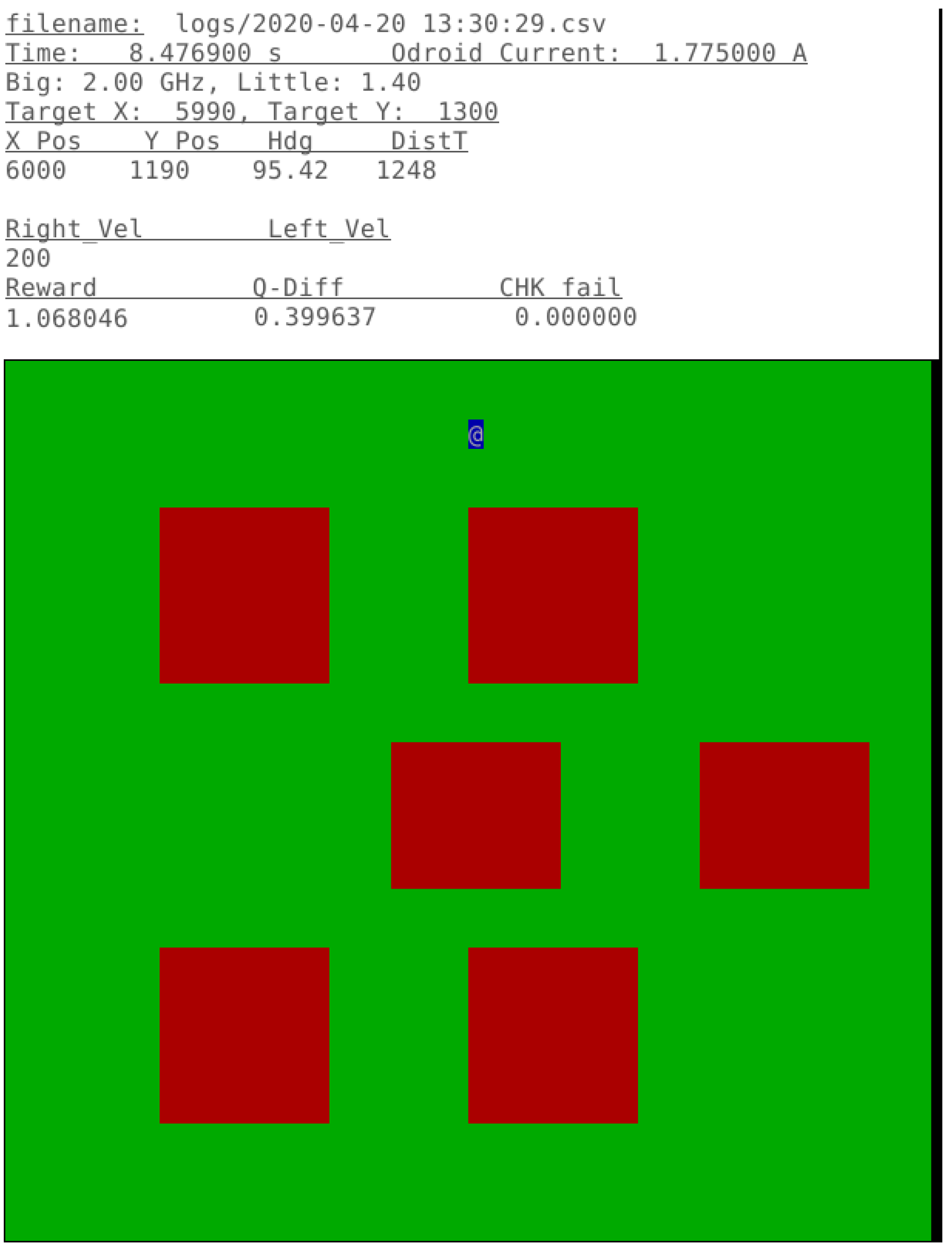
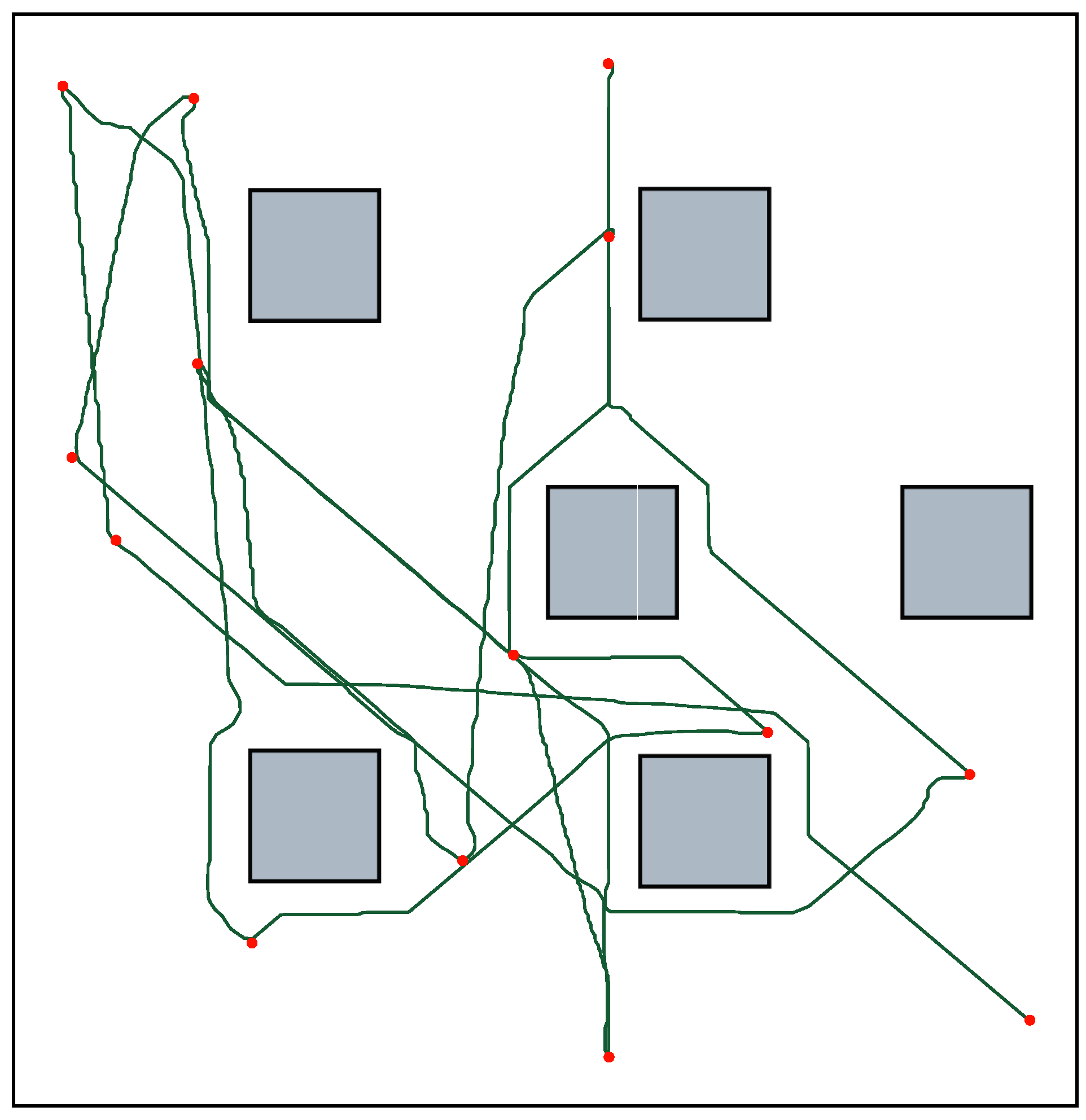
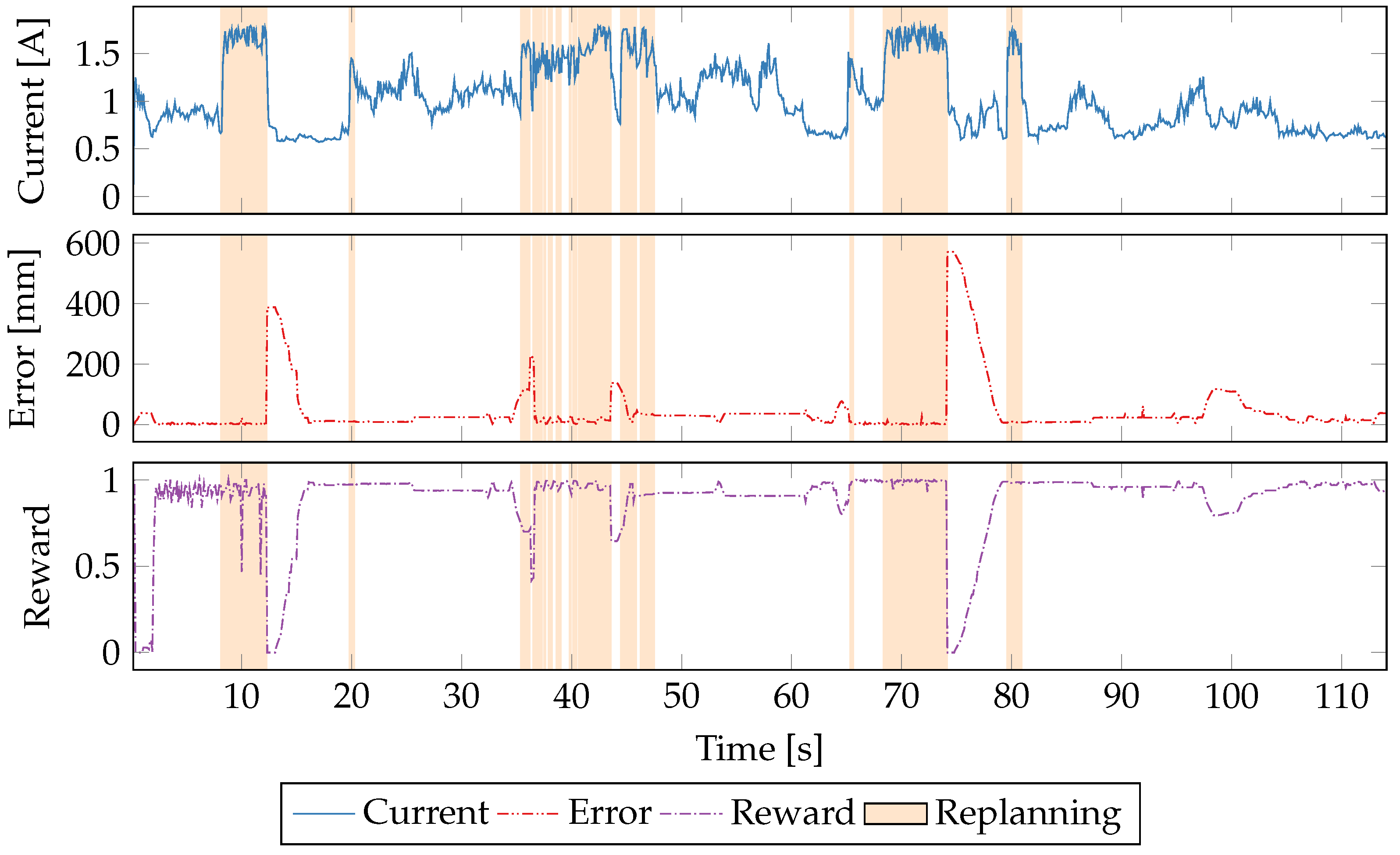
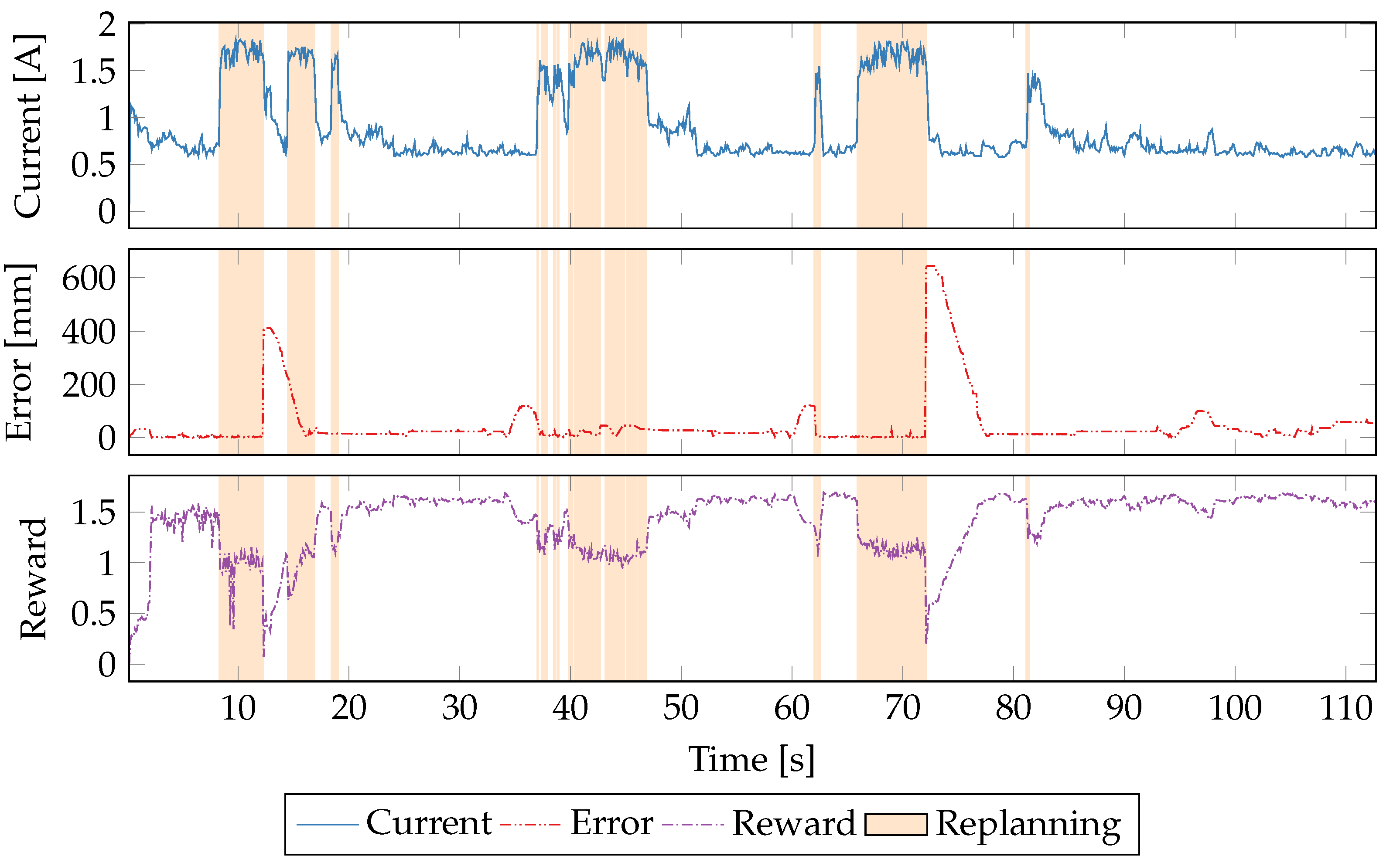
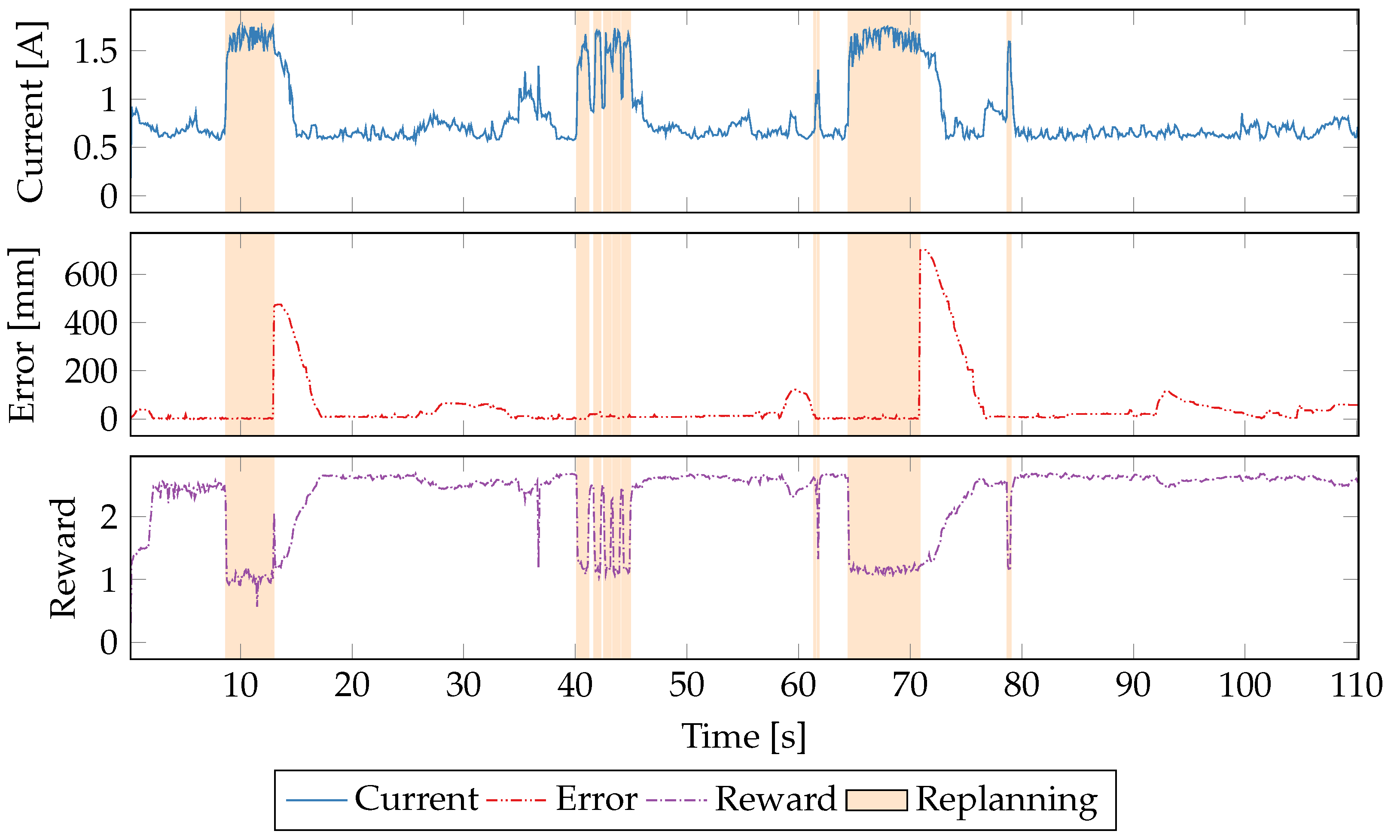
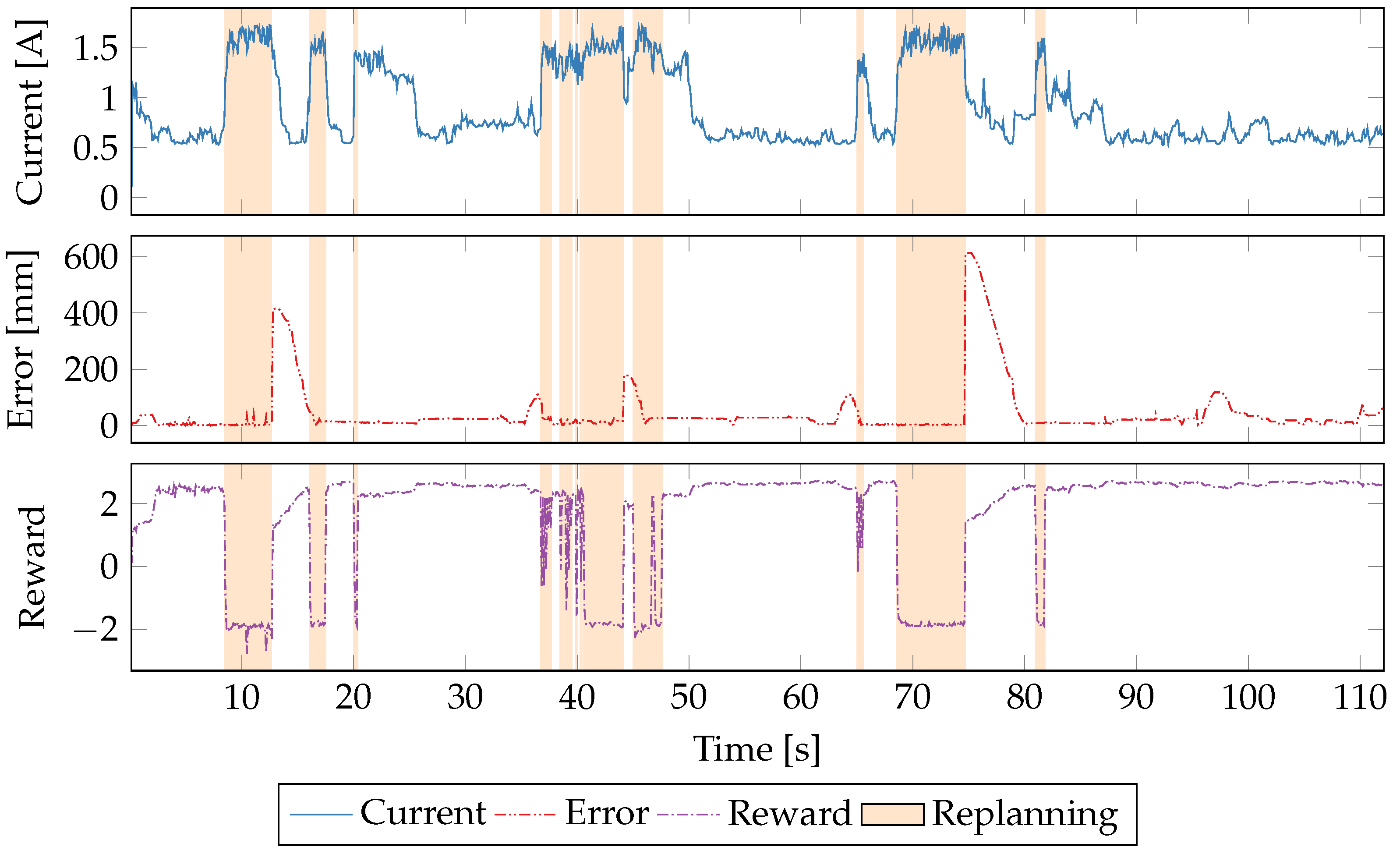
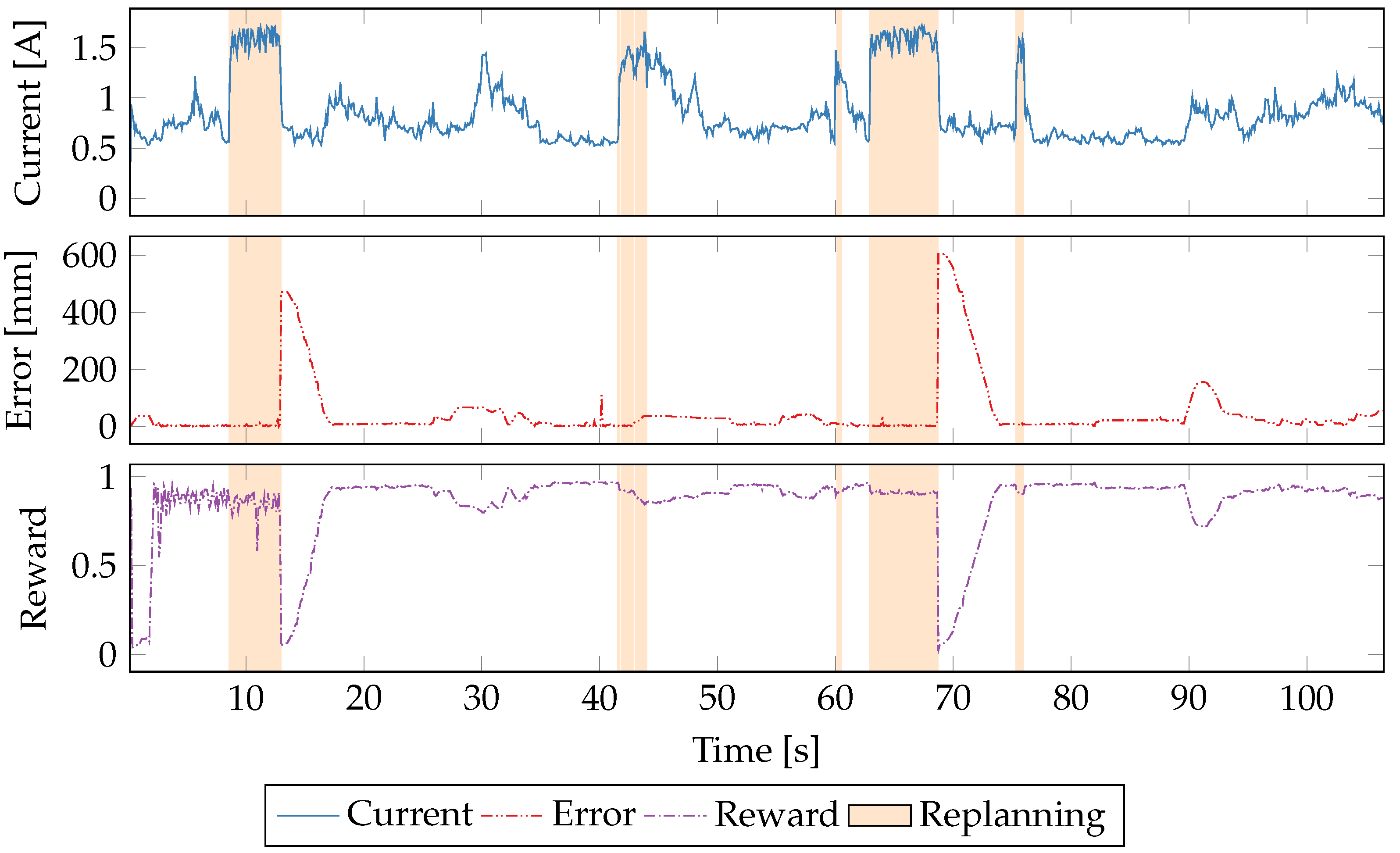
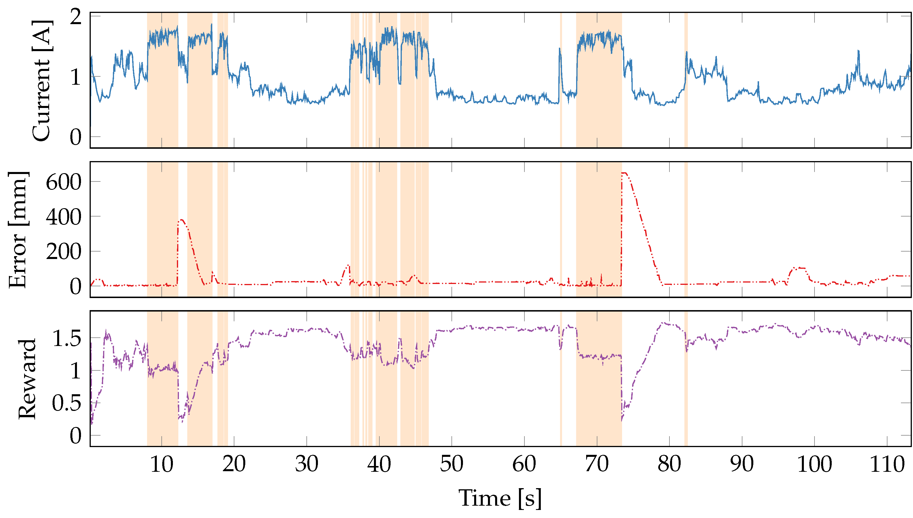
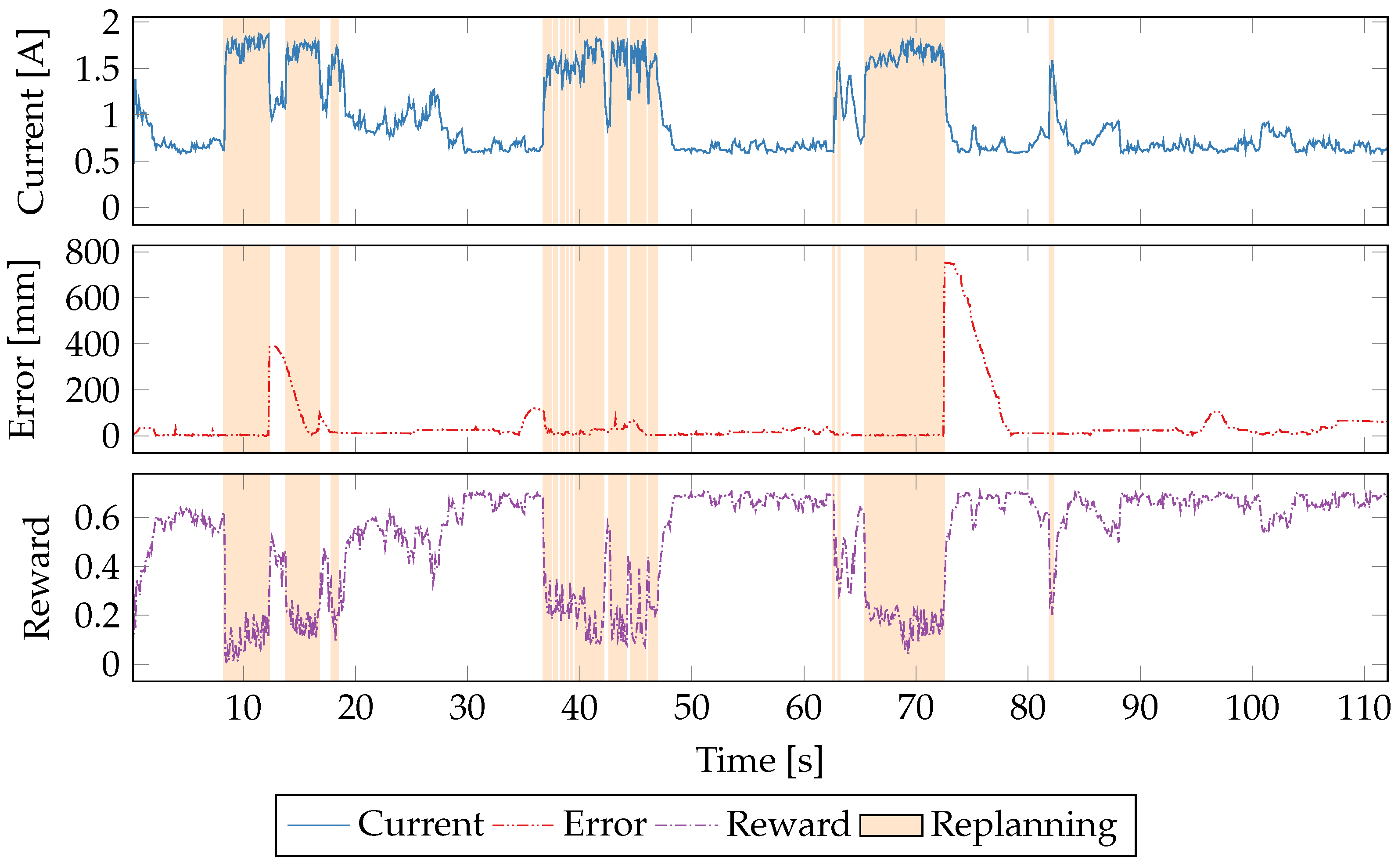
5.5. Time Series Evaluation

To better understand the behavior of the learners during the course of the experiments, we collected data at every update (10 ms) of the algorithm over the course of run. The previously presented data in Section 5.4 are 10-run averages, the time series data represent a single representative traversal of the course.

We will examine reward functions individually; however, the presentation of data is the same. The current (a stand-in for power since the voltage remains constant) is shown in blue and measured on the left-hand y-axis. Reward shares this axis and is shown in fuscia. The measured error from the desired path is shown in red and uses the right-hand y-axis and is measured in millimeters. When 2QoSM is in replanning mode, the graph is highlighted in peach.

Figure 9 shows the behavior of 2QoSM when the only goal is to minimize error. In aggregate, the error is lowest in the error-only reward function but, examining the time series data, it is not obvious why this is the case. Most likely, the application guidance from the navigation algorithm allows the 2QoSM to proactively power-up the cores to maximum performance, reducing the latency introduced by a sudden increase in computational intensity. This lower latency allows for a faster rerouting and thus a smaller divergence from the ideal path. However, this uncertainty in behavior demonstrates one of the shortcomings of Q-learning (and machine learning in general), namely, we can often get very good results but it is not always clear why they are good. Fortunately, using other reward functions, the learner’s behavior is much more clear.

It is much easier to see how the policy using a power-only reward function behaves in Figure 10. The learner capably decides that highest rewards come from aggressive CPU throttling. Even during the error spikes at 73 s, the power stays low. This is correct behavior in this specific situation because the error is due to drift from the path while calculating a new path. As soon as the path is calculated, the robot can refind the path just as quickly in low-power mode as in high-power. This behavior is quite similar to that of the situation-aware governor [45], but requires no understanding of the system itself nor any tuning of $K_p$ and $K_e$ parameters.

By adding path error back into the reward function, as shown in Figure 11, the learner behaves very similarly to using a power-only reward function. Again, the learner identifies that with a reduction in power, significant rewards are possible, and thus attempts to aggressively power-down the system when not replanning. Similarly, it does not respond to spikes in error. Even though in this situation, not responding to path drift is the correct behavior, in scenarios in which path error is due to CPU underperformance, the lack of reaction to the error could be seen as a failure. However, it is possible that if error due to CPU overutilization occurred, the characteristics and response to state changes would be different and the learner would learn the correct behavior. This is a topic for future research.

If we include in the reward function whether or not the robot is in replanning mode, we obtain the results shown in Figure 12. The motivation behind reducing the reward in replanning mode is to incentivize the learner to minimize the amount of time in replanning mode, and the only way to do this is to maximize CPU performance to quickly find the path. This reward function performs quite well overall, including when responding to increased error. By having three equal inputs to the reward, it may be diluting the influence of the $P_t$ term, thereby making the $E_t$ more important.

Because the goal of introducing the replanning mode r into the reward function was to limit the amount of time in replanning mode, we also evaluated an accumulating replanning variable $\sum r$ which reduces the reward by a greater amount the longer the robot remains in replanning mode. This makes it more “painful” for the algorithm to replan, with the goal of having the learner more aggressively attempt to get through the intensive section. Due to the high sampling frequency of the Q updates, we capped $\sum r$ so as not to completely overwhelm the reward function. Even with this protection, $\sum r$ clearly dominates the reward function shown in Figure 13 and seems to negatively affect the learner’s ability to reach an ideal power state.

While the various power-optimizing reward functions show improvement over traditional governors, the learner still has difficulty reacting to error, both due to drift during path recalculation and non-deterministic path error. In order to put more emphasis on the error portion of the reward function, we modified the sum of power and error to be weighted in favor of the error. The time-series measurements of the 1:10 power–error reward function are shown as Figure 14. From the fuscia plot of the reward function, it is clear that power dominates the reward function, however there is very little change in behavior when the error is high. This is further evidence of the challenges of using physical system error to train a power manager. Even with a discount factor $\gamma$ that favors future rewards over instantaneous ones, the learner still has difficulty finding actions that react to significant changes in error. That said, even with a 10x emphasis on error, simply having power in the reward function allows the learner to reduce power significantly.

Because error due to computational system latency lags the event itself due to the behavior of the physical robot, we attempt to slow down power observations by use of a moving average. We evaluated 10, 50 and 100-sample moving averages experimentally, but we only present the 10-sample moving average in Figure 15. Both 50 and 100-sample moving averages had worse performance than the 10-sample version without any recognizable reaction to the increasing error. Given the 10 ms sample time, the 10-sample moving average still reacts quite quickly to CPU state changes. This means that the learner is still able to obtain greater rewards by selecting lower-power states. However, without the instantaneous feedback from DVFS state changes, the learner seems less effective and thus the power reduction is less significant. Furthermore, as seen at $t=$ 83 s, power consumption increases without any identifiable cause. This is likely the fault of the delayed power observations making the learner less certain about the correct action to take.

6. Conclusions

This paper describes three significant results. First, we present a C-based Q-learning quality-of-service manager that learns a power management policy by taking input from both the application and computing platform. This 2QoSM is a drop-in replacement in the software framework described in [45], allowing for quick development and deployment on an autonomous robot. Depending on the reward function used, the 2QoSM reduced power by 38.7–42.6% over the Linux on-demand governor and 4.0–10.2% over the situation-aware governor. With the addition of an error term in the reward function, 2QoSM reduces error by 4.6% to 8.9% compared to these governors. In addition, this technique can be easily adapted for different systems by adjusting the reward functions, state vector and learning parameters.

Second, we provide further evidence for the value of reusable software abstractions provided by the software framework. The Q-learner was added to the existing infrastructure without changes to the framework itself. In addition, we did not have to tune the governor based upon metrics or states. All the developer must provide is a discretization of the state variables and enumeration of the possible actions. This simplicity enables the use of complex or novel machine learning algorithms as well as easier porting to different hardware and applications. System programmers are not restricted to a specific learner, or indeed even to a specific control paradigm.

Three, we want to emphasize the challenges inherent in using even relatively simple machine learning techiques. While Q-learning is a well-understood and often-used algorithm, the policies it develops are much more opaque. Increasingly, there is a trade-off that must be made between ease-of-use of well-performing machine learning and human understanding and control of these complex systems.

Future work continues in three different areas. First, Q-Learning has difficulty learning an optimal policy when the desired quality-of-service metric/reward is not directly changed by the actions performed. In our case, the error encountered is not always due to the actions taken by the computing platform; therefore, it is difficult to determine what the right decision is when confronted with error. In addition, when there is a portion of the reward (e.g., power) that is directly and instantaneously affected by the actions, this tends to dominate the learner’s policy. Some of these can be ameliorated with a more thorough parametric search of the learner itself, examining a larger range of discount factors, learning rates and actions. We are exploring other reinforcement learning techniques such as $Q\left(\lambda \right)$ and Deep Q-Learning. The former allows for a longer history of actions to influence the policy and the latter allows for a larger state space to be taken into account.

Second, we are evaluating the framework on other systems that share the properties of different performance modes and a metric of progress. Possible targets include OLTP workloads (e.g., transaction latency as a metric) or video encoding/decoding with quality/framerate as a changeable operating mode and signal-to-noise ratio as a metric of performance.

Finally, we are looking at further abstractions of the hardware system which may allow for a more universal framework for policy development and deployment. If there were detailed semantics for describing the hardware as seen by systems software, we can more thoroughly use the available hardware for the creation of policies for not only power management, but allocation and scheduling.

References

1. Govil, K.; Chan, E.; Wasserman, H. Comparing Algorithm for Dynamic Speed-setting of a Low-power CPU. In Proceedings of the MobiCom ’95: 1st Annual International Conference on Mobile Computing and Networking, Berkeley, CA, USA, 13–15 November 1995; ACM: New York, NY, USA, 1995; pp. 13–25. [Google Scholar] [CrossRef]
2. Hu, Z.; Buyuktosunoglu, A.; Srinivasan, V.; Zyuban, V.; Jacobson, H.; Bose, P. Microarchitectural Techniques for Power Gating of Execution Units. In Proceedings of the 2004 International Symposium on Low Power Electronics and Design (ISLPED ’04), Newport Beach, CA, USA, 11 August 2004; Association for Computing Machinery: New York, NY, USA, 2004; pp. 32–37. [Google Scholar] [CrossRef]
3. Agarwal, K.; Deogun, H.; Sylvester, D.; Nowka, K. Power gating with multiple sleep modes. In Proceedings of the 7th International Symposium on Quality Electronic Design (ISQED’06), San Jose, CA, USA, 27–29 March 2006. [Google Scholar] [CrossRef]
4. Liu, S.; Pattabiraman, K.; Moscibroda, T.; Zorn, B.G. Flikker: Saving DRAM Refresh-Power through Critical Data Partitioning. In Proceedings of the Sixteenth International Conference on Architectural Support for Programming Languages and Operating Systems, Newport Beach, CA, USA, 5–11 March 2011; Association for Computing Machinery: New York, NY, USA, 2011; pp. 213–224. [Google Scholar] [CrossRef]
5. Liu, J.; Jaiyen, B.; Veras, R.; Mutlu, O. RAIDR: Retention-Aware Intelligent DRAM Refresh. SIGARCH Comput. Archit. News 2012, 40, 1–12. [Google Scholar] [CrossRef]
6. Li, K.; Kumpf, R.; Horton, P.; Anderson, T. A Quantitative Analysis of Disk Drive Power Management in Portable Computers. In Proceedings of the USENIX Winter 1994 Technical Conference (WTEC’94), San Francisco, CA, USA, 17–21 January 1994; USENIX Association: Berkeley, CA, USA, 1994; p. 22. [Google Scholar]
7. Intel Corporation. Intel Automated Relational Knowledge Base (ARK). 2020. Available online: https://ark.intel.com/content/www/us/en/ark.html (accessed on 31 January 2022).
8. Ghose, S.; Yaglikçi, A.G.; Gupta, R.; Lee, D.; Kudrolli, K.; Liu, W.X.; Hassan, H.; Chang, K.K.; Chatterjee, N.; Agrawal, A.; et al. What Your DRAM Power Models Are Not Telling You: Lessons from a Detailed Experimental Study. Proc. ACM Meas. Anal. Comput. Syst. 2018, 2, 1–41. [Google Scholar] [CrossRef]
9. Ahmadoh, E.; Tawalbeh, L.A. Power consumption experimental analysis in smart phones. In Proceedings of the 2018 Third International Conference on Fog and Mobile Edge Computing (FMEC), Barcelona, Spain, 23–26 April 2018; pp. 295–299. [Google Scholar] [CrossRef]
10. Riaz, M.N. Energy consumption in hand-held mobile communication devices: A comparative study. In Proceedings of the 2018 Int’l Conference on Computing, Mathematics and Engineering Technologies (iCoMET), Sukkur, Pakistan, 3–4 March 2018; pp. 1–5. [Google Scholar] [CrossRef]
11. Bai, G.; Mou, H.; Hou, Y.; Lyu, Y.; Yang, W. Android Power Management and Analyses of Power Consumption in an Android Smartphone. In Proceedings of the 2013 IEEE 10th International Conference on High Performance Computing and Communications & 2013 IEEE International Conference on Embedded and Ubiquitous Computing, Zhangjiajie, China, 13–15 November 2013; pp. 2347–2353. [Google Scholar] [CrossRef]
12. Martinez, B.; Montón, M.; Vilajosana, I.; Prades, J.D. The Power of Models: Modeling Power Consumption for IoT Devices. IEEE Sens. J. 2015, 15, 5777–5789. [Google Scholar] [CrossRef] [Green Version]
13. Intel Corporation and Microsoft Corporation. Advanced Power Management (APM) BIOS Interface Specification v1.2. Available online: https://cupdf.com/document/advanced-power-management-apm-bios-interface-specification-revision-12-february.html (accessed on 31 January 2022).
14. UEFI Forum. Advanced Configuration and Power Interface Specification v6.3; UEFI Forum: Beaverton, OR, USA, 2019. [Google Scholar]
15. Chandrakasan, A.P.; Sheng, S.; Brodersen, R.W. Low-power CMOS digital design. IEICE Trans. Electron. 1992, 27, 473–484. [Google Scholar] [CrossRef] [Green Version]
16. Wakerly, J. Digital Design: Principles and Practices, 4th ed.; Prentice-Hall, Inc.: Hoboken, NJ, USA, 2005. [Google Scholar]
17. Kim, N.S.; Austin, T.; Baauw, D.; Mudge, T.; Flautner, K.; Hu, J.S.; Irwin, M.J.; Kandemir, M.; Narayanan, V. Leakage current: Moore’s law meets static power. Computer 2003, 36, 68–75. [Google Scholar] [CrossRef]
18. Veendrick, H.J.M. Short-circuit dissipation of static CMOS circuitry and its impact on the design of buffer circuits. IEEE J. Solid-State Circuits 1984, 19, 468–473. [Google Scholar] [CrossRef] [Green Version]
19. Pallipadi, V.; Starikovskiy, A. The ondemand governor. In Proceedings of the Linux Symposium, Ottawa, ON, Canada, 19–22 July 2006; Volume 2, pp. 215–230. [Google Scholar]
20. Brodowsk, D.; Golde, N.; Wysocki, R.J.; Kumar, V. CPU Frequency and Voltage Scaling Code in the Linux(TM) Kernel. Available online: https://www.mikrocontroller.net/attachment/529080/Linux-CPU-freq-governors.pdf (accessed on 31 January 2022).
21. Ahmed, S.; Ferri, B.H. Prediction-Based Asynchronous CPU-Budget Allocation for Soft-Real-Time Applications. IEEE Trans. Comput. 2014, 63, 2343–2355. [Google Scholar] [CrossRef]
22. Ge, R.; Feng, X.; Feng, W.C.; Cameron, K.W. CPU MISER: A Performance-Directed, Run-Time System for Power-Aware Clusters. In Proceedings of the 2007 Int’l Conference on Parallel Processing (ICPP 2007), Xi’an, China, 10–14 September 2007. [Google Scholar] [CrossRef] [Green Version]
23. Deng, Q.; Meisner, D.; Bhattacharjee, A.; Wenisch, T.F.; Bianchini, R. CoScale: Coordinating CPU and Memory System DVFS in Server Systems. In Proceedings of the 2012 45th Annual IEEE/ACM International Symposium on Microarchitecture, Vancouver, BC, Canada, 1–5 December 2012; pp. 143–154. [Google Scholar] [CrossRef]
24. David, H.; Gorbatov, E.; Hanebutte, U.R.; Khanna, R.; Le, C. RAPL: Memory power estimation and capping. In Proceedings of the 2010 ACM/IEEE International Symposium on Low-Power Electronics and Design (ISLPED), Austin, TX, USA, 18–20 August 2010; pp. 189–194. [Google Scholar] [CrossRef]
25. Albers, S.; Antoniadis, A. Race to Idle: New Algorithms for Speed Scaling with a Sleep State. ACM Trans. Algorithms 2014, 10, 1–31. [Google Scholar] [CrossRef]
26. Das, A.; Merrett, G.V.; Al-Hashimi, B.M. The slowdown or race-to-idle question: Workload-aware energy optimization of SMT multicore platforms under process variation. In Proceedings of the 2016 Design, Automation Test in Europe Conference Exhibition (DATE), Dresden, Germany, 14–18 March 2016; pp. 535–538. [Google Scholar]
27. Awan, M.A.; Petters, S.M. Enhanced Race-To-Halt: A Leakage-Aware Energy Management Approach for Dynamic Priority Systems. In Proceedings of the 23rd Euromicro Conference on Real-Time Systems, Porto, Portugal, 5–8 July 2011; pp. 92–101. [Google Scholar] [CrossRef]
28. Giardino, M.; Ferri, B. Correlating Hardware Performance Events to CPU and DRAM Power Consumption. In Proceedings of the 2016 IEEE International Conference on Networking, Architecture and Storage (NAS), Long Beach, CA, USA, 8–10 August 2016; pp. 1–2. [Google Scholar] [CrossRef]
29. Kumar, K.; Doshi, K.; Dimitrov, M.; Lu, Y.H. Memory energy management for an enterprise decision support system. In Proceedings of the IEEE/ACM International Symposium on Low Power Electronics and Design, Fukuoka, Japan, 1–3 August 2011; pp. 277–282. [Google Scholar] [CrossRef]
30. Tolentino, M.E.; Turner, J.; Cameron, K.W. Memory MISER: Improving Main Memory Energy Efficiency in Servers. IEEE Trans. Comput. 2009, 58, 336–350. [Google Scholar] [CrossRef]
31. Ghosh, M.; Lee, H.H.S. Smart Refresh: An Enhanced Memory Controller Design for Reducing Energy in Conventional and 3D Die-Stacked DRAMs. In Proceedings of the 40th Annual IEEE/ACM International Symposium on Microarchitecture (MICRO 40), Chicago, IL, USA, 1–5 December 2007; IEEE Computer Society: Washington, DC, USA, 2007; pp. 134–145. [Google Scholar] [CrossRef] [Green Version]
32. Qureshi, M.K.; Srinivasan, V.; Rivers, J.A. Scalable High Performance Main Memory System Using Phase-change Memory Technology. In Proceedings of the ISCA ’09: 36th Annual International Symposium on Computer Architecture, Austin, TX, USA, 20–24 June 2009; ACM: New York, NY, USA, 2009; pp. 24–33. [Google Scholar] [CrossRef]
33. Giardino, M.; Doshi, K.; Ferri, B. Soft2LM: Application Guided Heterogeneous Memory Management. In Proceedings of the 2016 IEEE International Conference on Networking, Architecture and Storage (NAS), Long Beach, CA, USA, 8–10 August 2016; pp. 1–10. [Google Scholar] [CrossRef]
34. Li, B.; León, E.A.; Cameron, K.W. COS: A Parallel Performance Model for Dynamic Variations in Processor Speed, Memory Speed, and Thread Concurrency. In Proceedings of the HPDC ’17: 26th International Symposium on High-Performance Parallel and Distributed Computing, Washington, DC, USA, 26–30 June 2017; ACM: New York, NY, USA, 2017; pp. 155–166. [Google Scholar] [CrossRef]
35. Li, B.; Nahrstedt, K. A control-based middleware framework for quality-of-service adaptations. IEEE J. Sel. Areas Commun. 1999, 17, 1632–1650. [Google Scholar] [CrossRef] [Green Version]
36. Zhang, R.; Lu, C.; Abdelzaher, T.F.; Stankovic, J.A. ControlWare: A Middleware Architecture for Feedback Control of Software Performance. In Proceedings of the 22nd International Conference on Distributed Computing Systems (ICDCS’02), Vienna, Austria, 2–5 July 2002; IEEE Computer Society: Washington, DC, USA, 2002; pp. 301–310. [Google Scholar]
37. Hoffmann, H. CoAdapt: Predictable Behavior for Accuracy-Aware Applications Running on Power-Aware Systems. In Proceedings of the 2014 26th Euromicro Conference on Real-Time Systems, Madrid, Spain, 8–11 July 2014; pp. 223–232. [Google Scholar] [CrossRef]
38. Shahhosseini, S.; Moazzemi, K.; Rahmani, A.M.; Dutt, N. On the feasibility of SISO control-theoretic DVFS for power capping in CMPs. Microprocess. Microsyst. 2018, 63, 249–258. [Google Scholar] [CrossRef]
39. Rahmani, A.M.; Donyanavard, B.; Mück, T.; Moazzemi, K.; Jantsch, A.; Mutlu, O.; Dutt, N. SPECTR: Formal Supervisory Control and Coordination for Many-core Systems Resource Management. In Proceedings of the ASPLOS ’18: Twenty-Third International Conference on Architectural Support for Programming Languages and Operating Systems, Williamsburg, VA, USA, 24–28 March 2018; ACM: New York, NY, USA, 2018; pp. 169–183. [Google Scholar] [CrossRef]
40. Muthukaruppan, T.S.; Pricopi, M.; Venkataramani, V.; Mitra, T.; Vishin, S. Hierarchical Power Management for Asymmetric Multi-core in Dark Silicon Era. In Proceedings of the DAC ’13: 50th Annual Design Automation Conference, Austin, TX, USA, 29 May–7 June 2013; ACM: New York, NY, USA, 2013; pp. 174:1–174:9. [Google Scholar] [CrossRef]
41. Somu Muthukaruppan, T.; Pathania, A.; Mitra, T. Price Theory Based Power Management for Heterogeneous Multi-cores. SIGARCH Comput. Archit. News 2014, 42, 161–176. [Google Scholar] [CrossRef]
42. Giardino, M.; Maxwell, W.; Ferri, B.; Ferri, A. Speculative Thread Framework for Transient Management and Bumpless Transfer in Reconfigurable Digital Filters. In Proceedings of the 2018 Annual American Control Conference (ACC), Milwaukee, WI, USA, 27–29 June 2018; pp. 3786–3791. [Google Scholar] [CrossRef] [Green Version]
43. Imes, C.; Kim, D.H.K.; Maggio, M.; Hoffmann, H. POET: A portable approach to minimizing energy under soft real-time constraints. In Proceedings of the 21st IEEE Real-Time and Embedded Technology and Applications Symposium, Seattle, WA, USA, 13–16 April 2015; pp. 75–86. [Google Scholar] [CrossRef]
44. Imes, C.; Hoffmann, H. Bard: A unified framework for managing soft timing and power constraints. In Proceedings of the 2016 International Conference on Embedded Computer Systems: Architectures, Modeling and Simulation (SAMOS), Agios Konstantinos, Greece, 17–21 July 2016; pp. 31–38. [Google Scholar] [CrossRef]
45. Giardino, M.; Klawitter, E.; Ferri, B.; Ferri, A. A Power- and Performance-Aware Software Framework for Control System Applications. IEEE Trans. Comput. 2020, 69, 1544–1555. [Google Scholar] [CrossRef]
46. Das, A.; Walker, M.J.; Hansson, A.; Al-Hashimi, B.M.; Merrett, G.V. Hardware-software interaction for run-time power optimization: A case study of embedded Linux on multicore smartphones. In Proceedings of the 2015 IEEE/ACM International Symposium on Low Power Electronics and Design (ISLPED), Rome, Italy, 22–24 July 2015; pp. 165–170. [Google Scholar]
47. Martinez, J.F.; Ipek, E. Dynamic Multicore Resource Management: A Machine Learning Approach. IEEE Micro 2009, 29, 8–17. [Google Scholar] [CrossRef]
48. Sheng, Y.; Shafik, R.A.; Merrett, G.V.; Stott, E.; Levine, J.M.; Davis, J.; Al-Hashimi, B.M. Adaptive energy minimization of embedded heterogeneous systems using regression-based learning. In Proceedings of the 2015 25th International Workshop on Power and Timing Modeling, Optimization and Simulation (PATMOS), Salvador, Brazil, 1–4 September 2015; pp. 103–110. [Google Scholar] [CrossRef] [Green Version]
49. Ye, R.; Xu, Q. Learning-Based Power Management for Multicore Processors via Idle Period Manipulation. IEEE Trans. Comput.-Aided Des. Integr. Circuits Syst. 2014, 33, 1043–1055. [Google Scholar] [CrossRef] [Green Version]
50. Shen, H.; Tan, Y.; Lu, J.; Wu, Q.; Qiu, Q. Achieving Autonomous Power Management Using Reinforcement Learning. ACM Trans. Des. Autom. Electron. Syst. 2013, 18, 1–32. [Google Scholar] [CrossRef]
51. Ge, Y.; Qiu, Q. Dynamic Thermal Management for Multimedia Applications Using Machine Learning. In Proceedings of the 48th Design Automation Conference (DAC ’11), San Diego, CA, USA, 5–9 June 2011; ACM: New York, NY, USA, 2011; pp. 95–100. [Google Scholar] [CrossRef]
52. Das, A.; Al-Hashimi, B.M.; Merrett, G.V. Adaptive and Hierarchical Runtime Manager for Energy-Aware Thermal Management of Embedded Systems. ACM Trans. Embed. Comput. Syst. 2016, 15, 1–25. [Google Scholar] [CrossRef] [Green Version]
53. Gupta, U.; Mandal, S.K.; Mao, M.; Chakrabarti, C.; Ogras, U.Y. A Deep Q-Learning Approach for Dynamic Management of Heterogeneous Processors. IEEE Comput. Archit. Lett. 2019, 18, 14–17. [Google Scholar] [CrossRef]
54. Bienia, C.; Kumar, S.; Singh, J.P.; Li, K. The PARSEC benchmark suite: Characterization and architectural implications. In Proceedings of the 17th International Conference on Parallel Architectures and Compilation Techniques, Toronto, ON, Canada, 25–29 October 2008; pp. 72–81. [Google Scholar]
55. Gupta, U.; Campbell, J.; Ogras, U.Y.; Ayoub, R.; Kishinevsky, M.; Paterna, F.; Gumussoy, S. Adaptive Performance Prediction for Integrated GPUs. In Proceedings of the 35th International Conference on Computer-Aided Design (ICCAD ’16), Austin, TX, USA, 7–10 November 2016; ACM: New York, NY, USA, 2016; pp. 1–8. [Google Scholar] [CrossRef]
56. Gupta, U.; Babu, M.; Ayoub, R.; Kishinevsky, M.; Paterna, F.; Ogras, U.Y. STAFF: Online Learning with Stabilized Adaptive Forgetting Factor and Feature Selection Algorithm. In Proceedings of the 2018 55th ACM/ESDA/IEEE Design Automation Conference (DAC), San Francisco, CA, USA, 24–28 June 2018; pp. 1–6. [Google Scholar] [CrossRef]
57. Watkins, C.J.C.H.; Dayan, P. Q-learning. Mach. Learn. 1992, 8, 279–292. [Google Scholar] [CrossRef]
58. Sutton, R.S.; Barto, A.G.; Williams, R.J. Reinforcement learning is direct adaptive optimal control. IEEE Control Syst. Mag. 1992, 12, 19–22. [Google Scholar] [CrossRef]
59. Chi-Hyon, O.; Nakashima, T.; Ishibuchi, H. Initialization of Q-values by fuzzy rules for accelerating Q-learning. In Proceedings of the 1998 IEEE International Joint Conference on Neural Networks Proceedings, World Congress on Computational Intelligence (Cat. No.98CH36227), Anchorage, AK, USA, 4–9 May 1998; Volume 3, pp. 2051–2056. [Google Scholar]
60. Song, Y.; Li, Y.; Li, C.; Zhang, G. An efficient initialization approach of Q-learning for mobile robots. Int. J. Control. Autom. Syst. 2012, 10, 166–172. [Google Scholar] [CrossRef]
61. Even-Dar, E.; Mansour, Y. Learning Rates for Q-learning. J. Mach. Learn. Res. 2004, 5, 1–25. [Google Scholar]
62. DFRobot. Cherokey 4WD Datasheet. Available online: https://wiki.dfrobot.com/Cherokey_4WD_Mobile_Platform__SKU_ROB0102_ (accessed on 27 March 2021).
63. DFRobot. ROMEO BLE Datasheet. Available online: https://wiki.dfrobot.com/RoMeo_BLE__SKU_DFR0305_ (accessed on 27 March 2021).
64. Roy, R.; Bommakanti, V. ODROID XU4 User Manual. Available online: https://magazine.odroid.com/wp-content/uploads/odroid-xu4-user-manual.pdf (accessed on 31 January 2022).
65. Gupta, U.; Patil, C.A.; Bhat, G.; Mishra, P.; Ogras, U.Y. DyPO: Dynamic Pareto-Optimal Configuration Selection for Heterogeneous MPSoCs. ACM Trans. Embed. Comput. Syst. 2017, 16, 1–20. [Google Scholar] [CrossRef]
66. Butko, A.; Bruguier, F.; Gamatie, A.; Sassatelli, G.; Novo, D.; Torres, L.; Robert, M. Full-System Simulation of big.LITTLE Multicore Architecture for Performance and Energy Exploration. In Proceedings of the 2016 IEEE 10th International Symposium on Embedded Multicore/Many-core Systems-on-Chip (MCSOC), Lyon, France, 21–23 September 2016; pp. 201–208. [Google Scholar]
67. Chung, H.; Kang, M.; Cho, H.D. Heterogeneous Multi-Processing Solution of Exynos 5 Octa with ARM® big.LITTLE™ Technology. Available online: https://s3.ap-northeast-2.amazonaws.com/global.semi.static/HeterogeneousMulti-ProcessingSolutionofExynos5OctawithARMbigLITTLETechnology.pdf (accessed on 31 January 2022).
68. ARM. big.LITTLE Technology: The Future of Mobile. Available online: https://img.hexus.net/v2/press_releases/arm/big.LITTLE.Whitepaper.pdf (accessed on 31 January 2022).
69. Likhachev, M.; Ferguson, D.; Gordon, G.; Stentz, A.; Thrun, S. Anytime Dynamic A*: An Anytime, Replanning Algorithm. In Proceedings of the 15th International Conference on Automated Planning and Scheduling, Monterey, CA, USA, 5–10 June 2005; pp. 262–271. [Google Scholar]
70. Paszke, A.; Gross, S.; Massa, F.; Lerer, A.; Bradbury, J.; Chanan, G.; Killeen, T.; Lin, Z.; Gimelshein, N.; Antiga, L.; et al. PyTorch: An Imperative Style, High-Performance Deep Learning Library. In Advances in Neural Information Processing Systems 32; Wallach, H., Larochelle, H., Beygelzimer, A., d’Alché-Buc, F., Fox, E., Garnett, R., Eds.; Curran Associates, Inc.: Red Hook, NY, USA, 2019; pp. 8024–8035. [Google Scholar]
71. Gough, B. GNU Scientific Library Reference Manual, 3rd ed.; Network Theory Ltd.: Scotland, Galloway, UK, 2009. [Google Scholar]
72. Murao, H.; Kitamura, S. Q-Learning with adaptive state segmentation (QLASS). In Proceedings of the 1997 IEEE International Symposium on Computational Intelligence in Robotics and Automation CIRA’97, ‘Towards New Computational Principles for Robotics and Automation’, Monterey, CA, USA, 10–11 July 1997; pp. 179–184. [Google Scholar]
73. Gama, J.; Torgo, L.; Soares, C. Dynamic Discretization of Continuous Attributes. In Proceedings of the Progress in Artificial Intelligence—IBERAMIA 98, Lisbon, Portugal, 5–9 October 1998; Springer: Berlin/Heidelberg, Germany, 1998; pp. 160–169. [Google Scholar]
74. Gonzalez, R.; Horowitz, M. Energy dissipation in general purpose microprocessors. IEEE J. Solid-State Circuits 1996, 31, 1277–1284. [Google Scholar] [CrossRef] [Green Version]
75. Brooks, D.M.; Bose, P.; Schuster, S.E.; Jacobson, H.; Kudva, P.N.; Buyuktosunoglu, A.; Wellman, J.; Zyuban, V.; Gupta, M.; Cook, P.W. Power-aware Microarchitecture: Design and modeling challenges for next-generation microprocessors. IEEE Micro 2000, 20, 26–44. [Google Scholar]
Figure 1. A high level view of the software framework architecture.
Jlpea 12 00029 g001
Figure 2. The robot.
Jlpea 12 00029 g002
Figure 3. A block diagram of the stacked architecture of the robot.
Jlpea 12 00029 g003
Figure 4. A screenshot of the console while the training is running.
Jlpea 12 00029 g004
Figure 5. During the 600 s training phase, the robot traversed to randomly selected points on a map with 6 obstacles. The red dots represent the target points.
Jlpea 12 00029 g005
Figure 6. The changing updates to the Q states is the metric used to evaluate the convergance of the policy.
Jlpea 12 00029 g006
Figure 7. This figure shows the distribution and magnitude of updates in the Q-matrix. Darker colors show a higher measured future reward Q while the lightest values generally show state–action pairs that were never reached.
Jlpea 12 00029 g007
Figure 8. The collected metrics of power, performance and runtime on the top, Energy-Error Delay Product [45] of the reward functions with different weights on the bottom.
Jlpea 12 00029 g008
Figure 9. A time series plot of a single run using the error-only reward function.
Jlpea 12 00029 g009
Figure 10. A time series plot of a single run using the power-only reward function.
Jlpea 12 00029 g010
Figure 11. A time series plot of a single run using a sum of power and error as the reward function.
Jlpea 12 00029 g011
Figure 12. A time series plot of a single run using a sum of power, error and replan as the reward function.
Jlpea 12 00029 g012
Figure 13. A time series plot of a single run using a ramping sum of power, error and replan as the reward function.
Jlpea 12 00029 g013
Figure 14. A time series plot of a single run using a weighted sum of power and error.
Jlpea 12 00029 g014
Figure 15. A single traversal of the course with error and 10-sample moving average of power reward function. 2 E t + P ¯ 10 .
Jlpea 12 00029 g015