Article

Intra- and Inter-Server Smart Task Scheduling for Profit and Energy Optimization of HPC Data Centers

1
Department of Computer Engineering, Rochester Institute of Technology, New York, NY 14623, USA
2
Department of Electronics and Computer Science (ECS), University of Southampton, Southampton SO171BJ, UK
3
School of Computer Science and Electronic Engineering (CSEE), University of Essex, Colchester CO43SQ, UK
4
Department of Electronic and Software Systems, University of Southampton, Southampton SO171BJ, UK
5
School of Software Engineering, South China University of Technology, Guangzhou 510006, China
*
Author to whom correspondence should be addressed.
These authors contributed equally to this work.
J. Low Power Electron. Appl. 2020, 10(4), 32; https://doi.org/10.3390/jlpea10040032
Submission received: 13 August 2020 / Revised: 26 September 2020 / Accepted: 29 September 2020 / Published: 14 October 2020

Abstract

:
Servers in a data center are underutilized due to over-provisioning, which contributes heavily toward the high-power consumption of the data centers. Recent research in optimizing the energy consumption of High Performance Computing (HPC) data centers mostly focuses on consolidation of Virtual Machines (VMs) and using dynamic voltage and frequency scaling (DVFS). These approaches are inherently hardware-based, are frequently unique to individual systems, and often use simulation due to lack of access to HPC data centers. Other approaches require profiling information on the jobs in the HPC system to be available before run-time. In this paper, we propose a reinforcement learning based approach, which jointly optimizes profit and energy in the allocation of jobs to available resources, without the need for such prior information. The approach is implemented in a software scheduler used to allocate real applications from the Princeton Application Repository for Shared-Memory Computers (PARSEC) benchmark suite to a number of hardware nodes realized with Odroid-XU3 boards. Experiments show that the proposed approach increases the profit earned by 40% while simultaneously reducing energy consumption by 20% when compared to a heuristic-based approach. We also present a network-aware server consolidation algorithm called Bandwidth-Constrained Consolidation (BCC), for HPC data centers which can address the under-utilization problem of the servers. Our experiments show that the BCC consolidation technique can reduce the power consumption of a data center by up-to 37%.

1. Introduction

High Performance Computing (HPC) data centers typically contain a large number of computing nodes each consisting of multiple processing cores. The size and performance of these systems continue to increase which causes concerns to be raised over higher energy requirements [1,2,3,4]. Research estimates that data centers worldwide account for 1.1–1.5% of global electricity use [5]. It is therefore important to take measure that reduce this energy consumption.
Different techniques have been proposed in the literature to improve the energy efficiency of the data center. Dynamic Power Management (DPM) and Dynamic Voltage Frequency Scaling (DVFS) are popular techniques to reduce the power consumption of under-utilized resources. Consolidation of virtual machines (VMs) running in different servers into fewer servers to enable aggressive DPM or DVFS has become a major focus area in the research community [6,7,8,9,10,11,12,13].
However, server-consolidation with the sole objective of power reduction can impact the performance of the HPC data center negatively if the network is incapable of supporting the resultant aggregated traffic patterns or hotspot scenarios [14]. Therefore, careful attention to the impact of consolidation on network performance is necessary.
HPC data centers maintain queues of jobs which arrive periodically and must schedule these jobs to be executed in order to produce a profit. It is common to assign values to jobs which imply their level of importance compared to other jobs: higher value equates to higher importance [15]. Value is typically assigned based on expected profit earned from the completion of the job. In HPC systems, the scheduling of jobs is influenced by their value; typically a resource management system will attempt to maximize its profits by allocating its limited resources to the highest-value jobs in the queue. This is especially true when jobs arrive at a rate higher than the rate at which the system can process and execute them. Typically, the value obtained by completion of a job is time-dependent which reflects the necessity to schedule as early as possible.
Existing approaches which optimize resource management use fast heuristics to very quickly find practical allocations for the dynamically arriving jobs. The use of heuristics over more complicated algorithms reduces overhead in the delay of allocations and also lowering the resource requirement of the resource management system itself. Research has also been conducted which considers profiling results from design-time testing to improve both the run-time computational complexity and the quality of the heuristics [16,17]. While the results of these researches show significant improvement over other approaches, the technique is only applicable in select situations due to the required accurate information and assumption that there is little deviation in resources required by the jobs in the system. The challenge to overcome these disadvantages is to design an algorithm that accounts for this variation and builds up a full history of information about jobs in real-time instead of requiring the information to exist already.
In an orthogonal direction, novel data center network (DCN) technologies, leveraging emerging interconnection paradigms such as millimeter-wave (mmWave) interconnects have been proposed to reduce the power consumption of the networking equipment [18,19]. Wireless data center architectures have been proposed where Top-of-Rack (ToR) switches are interconnected with mmWave links while the intra-rack communication is achieved through traditional Ethernet [20,21,22,23]. Alternatively, server-centric wireless DCNs where direct wireless links are used for server-to-server communication have also been designed [24,25]. These wireless data center architectures can be considered as viable alternate for traditional wired architecture for HPC computing for reducing even more power consumption. Furthermore, designing adequate server consolidation techniques can result in further power saving.
Contribution: This paper attempts to address this challenge by using ideas from reinforcement learning techniques and designing a novel server consolidation technique. The resource management system performs allocations that optimize both profit (value) and energy using a combination of light-weight heuristics and historic run-time results. The system considers the scheduling problem as a Multi-Armed Bandit (MAB) model where each individual job allocation is a possible action. The approach uses a novel algorithm, inspired by the Upper-Confidence Bound technique [26], collects profiling information at run-time (exploration) to optimize future allocations of jobs (exploitation). We also propose a network-aware approach to server-consolidation called Bandwidth Constrained Consolidation (BCC) and study its impact on a data center. While consolidating tasks can reduce the power consumption of data centers, due to the arrival of new tasks and completion of existing tasks, the consolidated utilization profile of the servers may change adversely affecting the power consumption over time. Hence, the BCC consolidation algorithm should be repeated periodically. Hence we also propose a method to find the optimal inter-consolidation time for a data center and derive a mathematical formulation to estimate the optimal inter-consolidation time. This will enable optimally scheduling consolidation in a data center without the need for extensive simulations and measurements to achieve the optimality.
Paper Organization: Section 2 presents work related to this paper. Section 3 introduces the problem, including the definition of a job and its value, the MAB model, and the model of HPC systems. The novel, reinforcement learning-based approach is introduced in Section 3.4. In Section 4 we introduce the network aware server consolidation technique, traffic model, our proposed algorithm, and mathematical model to estimate optimal inter-consolidation time. Experimental results are presented in Section 5 and Section 6 concludes the paper.

2. Related Work

It is proven that the use of market-inspired resource allocation heuristics provides promising results in the common situation that HPC systems are overloaded with more jobs than they can handle [27]. These heuristics use some implementation of a value for jobs, both fixed [28] and changing over time [15]. Most of them choose the highest value job first, which might consume too many resources, leaving limited resources for jobs arriving in the future. Therefore, resources required for each job should be optimized.
Other heuristics exist such as value density (value divided by resource requirement) which addresses the issue of the highest value job consuming too many resources [29,30,31]. This heuristic instead will prefer jobs which are small and have reasonably high value over very large jobs with high value. However, this heuristic, and others like it, do not consider energy consumption.
A number of reinforcement learning techniques were compared for scheduling tasks on large-scale distributed systems [32]. In this comparison, energy efficiency was considered by attempting to maximize CPU utilization. This intuitively increases energy efficiency by reducing the wasted energy of having CPUs powered on but in an idle state. Similar reinforcement learning techniques are explored for data centers [33]. However, these researches only considered the fulfillment of the service level agreement (SLA) which provides a fixed value when jobs are completed before a specified deadline. This research instead considers the common case where the value of a job changes gradually as a function of time, known as a value-curve. In addition, the energy efficiency optimization does not focus on the reduction of energy consumption directly.
A report identified that the use of profiling results in jointly optimizing the value and energy of a job [17]. Further research also expanded the optimizations to monitoring and adapting the allocations during tasks’ execution by migrating to a different set of resources [34]. Both approaches require profiling of jobs at design-time, and the latter also requires the ability for jobs to pause execution and resume on a different set of resources. In contrast, the bandit-based technique in this paper attempts to similarly predict the value and energy of jobs without relying on the assumptions that prior information is obtainable and migration of jobs is possible.
In a complementary direction, under-utilization of the servers in a data center has always been observed mainly due to the over-provisioning for the peak demand hours [35]. In [6], various formulations of the cost-aware application placement problem for servers were first introduced without considering network performance. Similarly, in [7], a system was proposed that optimizes power consumption, performance benefits, and transient costs incurred by server consolidation. In [8] an efficient power-aware resource scheduling strategy was proposed that reduces data center power consumption based on live VM migration. A framework for VM migration and placement was proposed in [9] considering both the network topology and network traffic demands to minimize energy consumption while satisfying as many network-demands as possible. In [10], energy-aware VM placement was proposed where application dependencies were considered to reduce network energy consumption. In [11], a network-aware VM consolidation scheme was proposed for solving combined VM consolidation problems to conserve the energy of the data center. In [12], a heuristic to control VM migration based on prioritizing VMs with steady capacity was proposed. In addition to server consolidation, an opportunistic approach to reduce power consumption is proposed in [36]. From all of these studies, it is clear that if an adequate consolidation algorithm can be designed, a significant amount of power reduction can be possible for the HPC data centers.
Orthogonally, various designs have been proposed to address DCN design issues such as energy consumption, cabling complexity, scalability, and over-subscription. One popular topology used today in data center networks is a fat-tree topology. To address oversubscription and other issues in wired DCNs many alternative DCN architectures have been proposed such as BCube, DCell, DOS, VL2, and Helios [35,37]. However, these innovations still rely on copper or optical cables and do not mitigate the challenges due to high power consumption, design, and maintenance of a DCN with physical links. To alleviate the issues of DCNs with power-hungry switching fabrics and bundles of cables wireless data centers with mm-wave inter-rack links are envisioned in [18,20,21]. Most of the recent works on wireless data centers propose interconnecting entire racks of servers as units with 60 GHz wireless links primarily in order to utilize the commodity Ethernet switching between servers inside individual racks [18]. Phased antenna arrays or directional horn antennas are used to establish wireless links between ToRs in the entire data center [21,22,23]. Line-of-Sight (LoS) communication paths are necessary between the antennas for reliable communication in a wireless data center [21]. In [25] a novel wireless DCN architecture, based on 60 GHz wireless links between the individual servers of namely, S2S-WiDCN was proposed which drastically reduces the power consumption of the network portion of the data center while sustaining comparable performance. Hence, adopting an adequate wireless architecture for the HPC environment can result in significant power saving.

3. System and Problem Definition for Scheduling Problem
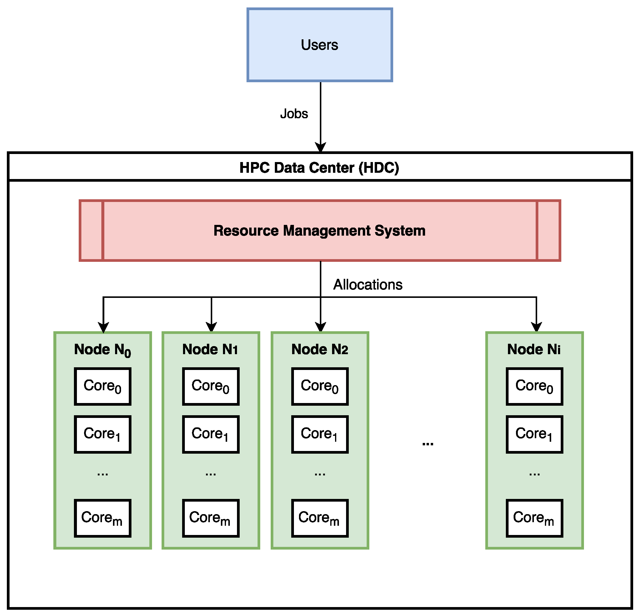
Figure 1 shows a simplified model of a typical HPC data center. Users submit their jobs to the data center which stores them in some data structure such as a queue until they can be allocated. Attempted allocations usually occur upon a change in the system, such as new jobs arriving or current allocations finishing which frees resources.

3.1. HPC System

The HPC Data Center (HDC) consists of a resource management system (RMS) connected to a number of different nodes ( N 0 , N 1 , , N i ) each containing a set of processing cores ( C o r e 0 , C o r e 1 , , C o r e m ). Each node represents a physical server in the data center being considered. The processing cores are homogeneous and communicate with each other via an interconnect. The RMS operates on its own set of resources and assigns arrived jobs to a set of cores within a single node. A single job is considered to use resources of a single node to avoid communication overhead between nodes. Further, to avoid migration overhead, it is assumed that jobs cannot be paused or migrated to a different set of resources during execution.
The HPC system is created in hardware as three Odroid-XU3 boards connected in a local area network (LAN). The CPU in these boards, Samsung Exynos5422, is powered by Arm® big.LITTLE™ architecture: four Cortex®-A15 cores at 2.0 GHz and four Cortex®-A7 cores at 1.4 GHz. As our model requires homogeneous cores in the nodes, only the A15 cores are used for job allocation. This conveniently allows the proposed RMS to execute solely on the A7 cores of one board instead of requiring separate hardware for its own set of resources. This represents a many HPC system with three nodes and many HPC systems are realized in the same way, where one node (server) or a set of cores act as the manager and other nodes (servers) are used to execute jobs after allocation [34]. Without the loss of generality and having better and more hardware availability, a large HPC system can be realized.

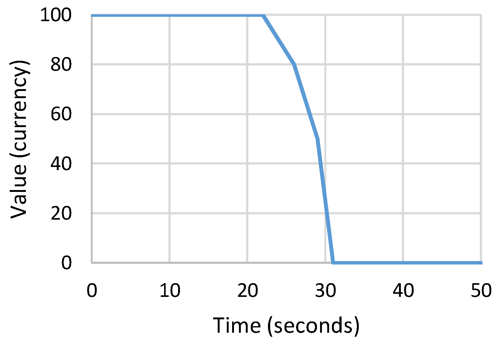
3.2. Jobs and Value Curves

Each job j is modeled as an tuple J = ( T ; A ) , where T is the arrival time of the job and A is the application to be executed in order to complete the job. Each job j also has its own value curve function V C j which converts a completion time of its execution to the value of the job to its user. These functions are typically monotonically-decreasing until reaching zero at a certain threshold of time, as shown in Figure 2. It is assumed that the value curves are pre-designed for each job and accurately reflect the economic importance to the user as the economic model is out of the scope of this paper.
The PARSEC benchmark suite was used as the set of applications to queue in the system. This is because the benchmark applications were designed to have a range of multi-threading and other resource requirements. The focus on emerging workloads means the jobs are representative of potential future workloads in all situations including but not exclusive to HPC systems. A number of applications from the suite were selected and value-curves were designed for each application based on testing the execution time across different numbers of cores. In particular, we considered PARSEC applications listed in Table 1. The table also represents the value-curve for each application in terms of execution time and the value achieved if job is executed by that time. The jobs are generated by selecting a random application from this list and assigning an arrival time to it. Short and long periods of no jobs arriving are created to realize periods of no users (such as nights and weekends); these allow the scheduler to “catch-up” on remaining jobs in the queue.
The value curves create a natural “soft deadline” which implies an ideal time for a job to finish, but also that violation of the deadline does not mean the job completion was irrelevant [38]. Instead, the value of the job is reduced depending on the extra time the user has had to wait for completion [15,39]. Major violations of the deadline will create no value for the user and therefore the energy consumed by the computation was wasted.

3.3. Problem Definition

The problem addressed by the paper is the allocation of jobs to a finite set of resources such that value obtained from completion of the jobs is maximized while energy consumption is minimized simultaneously. The problem is defined as follows:
  • Input: Job queue ( j 1 , , j n ), Value curve for each job V C j , Nodes within the HPC data center ( N 0 , , N i ).
  • Constraints: Restricted available cores on the nodes in H D C .
  • Objective: Jointly optimize overall value V a l t o t a l and energy consumption E t o t a l , by maximizing the quotient V a l t o t a l / E t o t a l .
The RMS needs to make very fast decisions on which node to allocate a job and which cores within that node should do the computation. It is assumed that any one job requires a minimum of one core and individual cores are never shared between multiple jobs.

3.4. Proposed Approach Based on Reinforcement Learning

This section describes the proposed approach. It first outlines the Adapted Multi-Armed Bandit (AMAB) model and discusses the assumptions and constraints of using such a model. Finally, the algorithm is described and explained in detail.

3.4.1. Adapted Multi-Armed Bandit Model

The MAB is a common model in reinforcement learning [40]. The model is of a game played in rounds from time t = 1 , , T . At each round, the player must select a single action from a known set of actions a t A . The environment then generates a reward r t R a t where R a t is an unknown probability distribution. The goal of the game is to maximize the cumulative reward t = 1 T r t by selecting actions which are likely to give high rewards. Due to the unknown nature of the reward distributions, players are required to first “explore” the possible actions to figure out the distributions before they can “exploit” the actions with the highest average probability.
For this paper, the problem is modeled as an adaptation of the MAB (AMAB) model. The possible actions are the different possible allocations of single jobs currently in the RMS queue, i.e., for each job there exists an action for each possible number of cores available for it to be allocated to. There may be multiple jobs of the same type in the queue which will create duplicate allocation possibilities, however, they will likely have different schedule delays. The rounds are the allocation stages, which occur at every change in the job queue or available resources. Therefore, the time step between each round varies significantly. The rewards are V a l j / E n e r g y j for each job after computation is complete.
The MAB model does not perfectly fit the described problem due to a number of assumptions: rounds are at discrete time steps, every action is available at every round, exactly one action is selected per round, and rewards are received instantly after selecting an action. As such, the problem model differs in the following ways: only a subset of all possible actions are available per round, multiple or no actions may be selected per round, and rewards at the start of some round in the future after selecting an action. To fit the model, this paper considers the use of the Upper Confidence Bound (UCB) algorithm [41], which is described in the next subsection.

3.4.2. Upper Confidence Bound Algorithm

The premise of the UCB algorithm is to model the uncertainty of information gathered through experimentation, allowing for exploitation to occur naturally as uncertainty is reduced. The UCB algorithm records the average rewards received for each action r i ^ alongside the number of times that action was chosen C i . It uses this count of previous rewards to calculate the uncertainty of the recorded average. This uncertainty and the average are combined to give a largest possible estimate for the actual mean of the reward distribution.
μ ^ i = r ^ i + 2 log ( 1 δ ) C i
where δ is a confidence value which is usually chosen or search for via parameter optimization. If the value is very small then the result is optimistic of a higher possible mean, while a high value implies less optimism. Possible values for δ are explored in experimentation. The algorithm simply chooses the action with the maximum μ ^ i as it is predicted to be the action with the best average rewards. As actions are repeated, the uncertainty represented by the second part of Equation (1) decreases due to the increased C i . However, the equation relies on C i 0 . Due to this requirement, the algorithm must first attempt each action at least once before estimating the means. Usually, implementations of UCB will spend the first k rounds, where k = | A | , selecting each action in turn. This gives an initial estimate for the average reward, though with a high uncertainty.
The final selection rule for UCB is as follows.
a t = arg max i μ ^ i , if t > k ; t , otherwise .
However, UCB makes various assumptions which do not fit our adapted model, such as that the rewards are in the interval [ 0 , 1 ] . The next section describes these assumptions and the required adaptations to be compatible with our HPC system.

3.4.3. Proposed Algorithm for Confidence-Based Approach

For the purpose of this paper, the algorithm created will be referred to as the Confidence-Based Approach (CBA) from its UCB inspiration. The CBA algorithm features a similar selection rule to UCB, however, it is modified to accommodate the new assumptions. The first modification is the selection: as every action is not available on every round, it cannot guarantee exploration of action t for t k . Instead, it always attempts to find the maximum possible mean from the available actions. When an action i with C i = 0 is encountered, the algorithm overrides the search for the maximum possible mean and instead allocates according to the job and number of cores of that action. This ensures full exploration of all possible actions that are encountered by the scheduler as soon as they are encountered.
The rewards from each action i are not guaranteed to be in the interval [ 0 , 1 ] either, as they are dependent on the user-specified value curve and the energy consumed by the system. This means that Equation (1) is not an accurate representation of the highest possible mean of an action. However, knowing the typical interval for the rewards can be used to scale the uncertainty part of the equation up to somewhat compensate for the difference. This can be done relatively easily using the specifications for the processing cores to obtain expected power and adding constraints to the maximum of the user specified value-curves. For our jobs, described in Section 3.2, typical reward values (>75%) were in the range [ 0 , 5 ] so we use a scaling multiplier of 5.
The reward, value divided by energy, is not strictly dependent on the job and number of allocated cores. Instead, it is derived from the sum of the computation time of the job, which is directly dependent on the allocation, and also the delay in scheduling of the job (time spent in the queue waiting). Due to this, the algorithm does not record the average reward from allocations but instead records the average computation time t ^ i and energy e ^ i . During the scheduling process, it combines this average computation time with the current schedule delay of the job to estimate the expected average value for the current moment in time. The average energy consumed is not affected by schedule delay so is used directly to calculate the expected reward.
The final scheduler is shown in Algorithm 1. The loop on line 1 of Algorithm 1 is the initialization of the data required to estimate the average rewards. The full list of possible allocations is the list of every combination of the type of job and number of cores, i.e., for each job there is an entry for every number of cores between its maximum number of cores and 1. Lines 7–31 show the allocation “rounds” in the bandit algorithm. First, all finished jobs are accounted for with appropriate updates of resources and historical data, then newly arrived jobs are added to the queue, and finally, the algorithm attempts to allocate jobs to newly freed resources if possible. The selection rule is on line 24 and is nearly identical to the rule described in Equation (2). Possible values for δ are explored during experimentation.
Algorithm 1: CBA Resource Allocation.
Jlpea 10 00032 i001
The Odroid boards used for the experiment support monitoring the energy consumption of the quad-core Cortex®-A15. The power sensor can only detect the energy consumed by the entire processor and not the individual cores. This means that it is impossible to get an accurate recording of energy use for a single job using less than four cores. Instead, the energy recorded over the duration of a job is simply an estimate and will vary based on other jobs running simultaneously on the nodes. Therefore, most jobs will have their energy consumption over-estimated and the reward V a l j / E n e r g y j will be underestimated. Experimentation for different levels of confidence using the δ parameter can give insight into how the variation in energy consumption estimates affects the learning algorithm. E n e r g y t o t a l for the full system can be still be recorded accurately for comparison.

4. System and Problem Definition for Network Aware Server Consolidation

To augment the efficient scheduling algorithm discussed above, we propose a server consolidation algorithm which will ensure optimal resource utilization under the performance constraints of the data center network.

4.1. Network Aware Server Consolidation

Server consolidation is a process where VMs running in one server are relocated to one or more different servers. However, as discussed earlier we propose a network-aware consolidation approach which takes into account the traffic interaction between the VMs running on the servers. In order for the VM migration approach to be network or traffic-aware, we first need to understand the nature of traffic interaction over the data center network.

4.2. Traffic Pattern Model

The traffic pattern in a data center network can be modeled in terms of multiple parameters such as flow arrival rates, flow injection rates, flow sizes, flow completion time and proportion of inter-rack and intra-rack flows [42]. In [25] a novel wireless DCN architecture, based on 60 GHz wireless links between the individual servers of namely, S2S-WiDCN was proposed which drastically reduces the power consumption of the network portion of the data center while sustaining comparable performance. The proposed network aware server consolidation can be adopted for S2S-WiDCN or conventional wired fat-tree data center networks. In the S2S-WiDCN, there are six separate directional antenna arrays in the vertical plane of the server, and another one array on the top of the server. Therefore, seven simultaneous links from a server can co-exist at the same time. We represent the number of possible simultaneous links per server as θ . Let F be a vector whose elements are the number of existing flows along each sector determined from the number of flows existing in each server based on their destinations and the routing protocol. Let f denote the traffic flow rate. It is to be noted, that the flow rate f, has a Gaussian distribution [42,43]. Therefore, to support 99.86% (one-sided z-distribution) of the flow rates, the required channel throughput should be
r = f μ + 3 σ F ,
where elements of the vector r , are the required channel throughput in each of the sectors and f μ + 3 σ is the value of the flow rate which is three standard deviations higher than the mean. For the S2S-WiDCN, to accommodate multiple channel access, a single 60 GHz IEEE802.11ad link is subdivided into n OFDM number of separate OFDM channels. Therefore, the bandwidth of each OFDM channel is given by,
B W = B 60 GHZ / n OFDM ,
where B 60 GHZ is the bandwidth of the single physical channel. For a wired network, B W would be equal to the bandwidth of the connected wire link. Therefore, to reduce the adverse effect of server consolidation on network performance, the following inequality must be satisfied for all wireless links or sectors from each server in the S2S-WiDCN,
r x < B W x
where r x is an element of r . If the inequality in (5) cannot be satisfied due to high flow rates, consolidation will result in worsening of data center network performance as discussed in the results.
Moreover, it has been observed from the measurement of a variety of data centers in [43], a large proportion of the server-to-server traffic flows, up to 80%, are intra-rack, meaning between servers in the same rack. Only a small remaining proportion of about 20% is inter-rack, or between servers in different racks. Therefore, to reduce the effective load on the network while consolidation, VMs that communicate more often should be migrated into the same physical server. Hence, in addition to reducing server underutilization, co-location of highly communicating VMs is also a desirable goal as it will reduce both power consumption and network traffic. This way, in our consolidation algorithm, we considered both the inequality of (5) and the proportion of inter and intra-rack traffic to make it network-aware.

4.3. The Network-Aware Consolidation Algorithm

The primary goal for consolidation is to reduce the total power consumption by reducing the number of active servers as well as network utilization. The underlying assumption is that the computational requirement for every VM running in the HPC data center and the injection rates of every flow from each VM is known and readily available. In a single server, multiple VMs can run at a single instance. However, during the server consolidation, we considered all the VMs running as a single entity, meaning if migration is possible, all the VMs running on the server would be migrated to the new physical server for consolidation. The migrations happen in online mode following live migration [10]. While this will reduce the granularity of the consolidation, it is a more scalable approach suitable for large data centers with thousands of servers. Moreover, the task-level granularity for a network-aware consolidation requires the knowledge of traffic flow per task, which is difficult to model, predict, or access in large data centers. Data center traffic rates are modeled usually among entire servers [42] limiting us to design consolidation algorithms at a server-level granularity.
We assume that every server has the same computational capacity and VMs running on a server utilizes a variable percent, collectively which can be represented by u. Let us assume that the maximum permissible utilization, without any significant degradation in performance or violation of legal contracts of any server, is D u . D u is a manufacturer specified parameter and can vary from model to model. The pseudo-code for implementing the BCC is shown in Algorithm 2. At first, all the servers running in the data center are divided into smaller clusters, such that servers within a cluster have a large number of flows exchanged among themselves, whereas servers in different clusters have a much smaller number of flows exchanged among them. Such a clustering places highly communicating servers in the same cluster. This intra-cluster consolidation reduces the communication among these highly communicating servers. This clustering is a Graph Partitioning Problem, which is to partition graph vertices into disjoint groups with minimum edge cut cost. The Kernighan–Lin algorithm [44] is adopted for the graph-partitioning tasks in our work. Here we treat servers as vertices and the number of flows going outside of the server as edge costs. After the partitioning, all the servers in each cluster are sorted according to their utilization u. The outer loop (line 5 in Algorithm 2) in the proposed algorithm chooses the candidate to migrate in the ascending order of utilization starting with the least utilized one. The inner loop (line 6 in Algorithm 2) chooses the destination to migrate in the descending order of utilization starting with the most utilized one. If the sum of the utilization of the candidates to migrate and the potential destination is less than D u and each element of the vector sum of their required injection rates is less than the channel throughput per OFDM channel, the candidate is migrated to the destination. This flow rate related condition for migration is informed by our traffic model related constraint in (5). After a successful migration, the inner loop is broken out of, to choose the next server in the outer loop for potential migration. If either of the two conditions fails, the inner loop continues till the list of servers for the potential destination is exhausted. For each completion of the inner loop, the outer loop progresses to the next candidate for migration.
Algorithm 2: Algorithm for Bandwidth-Constrained Consolidation (BCC).
Jlpea 10 00032 i002
The necessary steps of the migration function (Migrate) used in the pseudo-code of BCC Algorithm 2 are shown in Algorithm 3. The function migrates server a to server b. At first, all the VMs running in migrating server a is migrated in the destination server b. So the utilization of the destination server increases which is the summation of the utilization of both the servers. Vector r b is updated based on all the flows running on server b post migration. After successful migration, server a is put into the PowerNap state [45] having zero utilization. In the PowerNap state, most of the components of the server are powered down except the network interface card (NIC), the wireless transceivers, and a small portion of the CPU to get the signal for waking up when required.
Algorithm 3: Migration Function.
Jlpea 10 00032 i003

4.4. Complexity Analysis

Optimizing the performance of the scheduler in the data center has been a major research focus area for the last few years [46]. The calculation for the consolidation algorithm operations take place on the scheduler. The complexity of server consolidation over the entire data center to provide the optimal solution using exhaustive search method is O ( N N ) where N is the total number of servers in the entire data center. This is because N set of VMs can be potential candidates for migration to N servers in N ways. Therefore, each of N set of VMs has N options for potential migrations and for each of the N such scenarios the other sets of VMs also have all N options to create each possible migration scenario. However, this complexity is too high even for moderately large data centers. Therefore, we compare our proposed BCC consolidation algorithm with the Clustered Exhaustive Search (CES) algorithm, which finds the optimal migration within each cluster using the exhaustive search. We have adopted the Kernighan–Lin algorithm to do the clustering in the beginning of the BCC consolidation. If all the servers are equiprobable to have links between themselves, the computational complexity becomes O ( N 2 log N ) [44]. If the average number of servers in a cluster is n and if the number of the clusters formed is m, the computational complexity of the CES algorithm after clustering is O ( m n n ) and is an np-hard problem. With the clustering, the complexity of the CES algorithm is O ( N 2 log N + n n m ) . On the contrary, for the BCC algorithm, inside each cluster, the servers are sorted according to their utilization having a complexity of O ( n log n ) using merge sort [47]. Next, the two loops for finding the source and destination of the migration has the complexity of O ( n 2 ) in the worst case. So the overall complexity of BCC for all m clusters becomes O ( N 2 log N + m n log n + m n 2 ) . Therefore, BCC has a much lower complexity compared to the overall exhaustive search algorithm. As the clustering is similar in both CES and BCC, the difference in their complexity comes from the mechanism of determining candidates for migration. The complexity of BCC after clustering is O ( m n log n + m n 2 ) O ( m n 2 ) which, is lower than that of the CES after clustering.

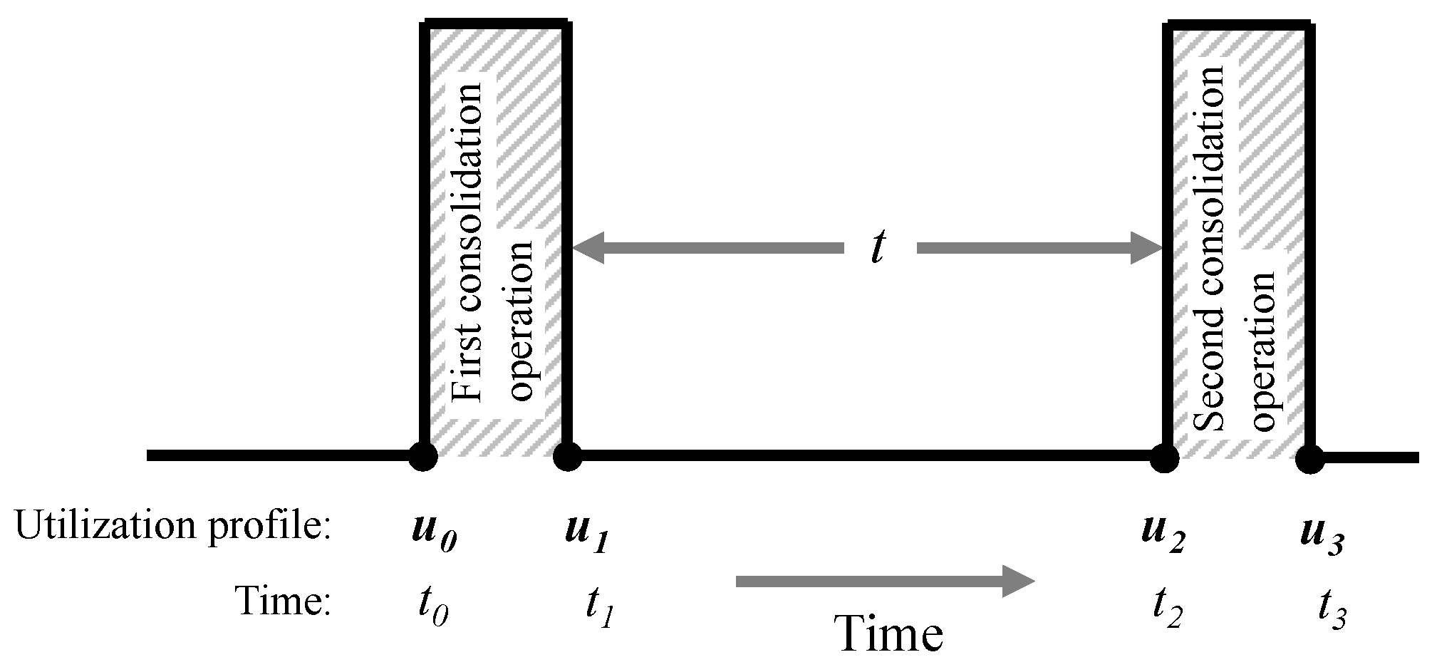
4.5. Optimizing the Inter-Consolidation Time

Due to the arrival of new tasks and the completion of existing tasks, the consolidated utilization profile of the servers may change over time. Therefore, the power consumption of the HPC data center may be adversely affected over time. Hence, the BCC consolidation algorithm should be repeated periodically. Repeating the consolidation too often might not reduce the total power consumption enough to justify the additional network traffic introduced as a result of the consolidation. On the contrary, delaying the consolidation can adversely affect the potential opportunity to save power. Hence, to determine the optimal time interval between two consecutive consolidations, an appropriate cost function, to capture the trade-off between power savings and network traffic is required. We define the expected value of the time-dependent cost function C ( t ) for inter consolidation time interval as
C ( t ) = κ E [ A ( t ) ] E [ B ( t ) ] ,
where A ( t ) is migration cost related to the network traffic which represents the total traffic movement for the consolidation operation, B ( t ) is the total power saving due to the consolidation, t represents the time interval between two consecutive consolidation operation, and κ is a scaling constant which captures the relative significance of network traffic and power savings. E [ · ] represents the expected value and is necessary as random task arrivals and completion make A ( t ) and B ( t ) random processes. At the optimal inter-consolidation time interval of t * , the cost C ( t ) should have the minimum value, that is,
t * = argmin t R C ( t )
Figure 3 represents the timeline for the consolidation operation which shows two consecutive consolidation operations. u denotes the utilization profile of all the servers in the HPC data center, where u = [ u 1 , u 2 , , u N ] T R + N if N is the total number of servers in the data center. At time t 0 , when the utilization profile is u 0 , first consolidation operation takes place, and immediately after the consolidation, at time t 1 , the utilization profile of the servers becomes u 1 . After t seconds at t 2 the utilization profile of the servers becomes u 2 and a second consolidation is carried out which is completed at t 3 with a final utilization profile of u 3 . Hence, it can be written that, u 1 = Γ u 0 and u 3 = Γ u 2 , where Γ represents the consolidation operation. Furthermore, it holds that,
u 2 = u 1 + δ t ,
where [ δ ] i is the task increase rate. A ( t ) is directly related to the amount of traffic transferred through the network for the migration. If the average size of traffic per migration is ν , then A ( t ) can be represented by,
A ( t ) = ν u 1 + δ t 0 Γ ( u 1 + δ t ) 0 ,
where · 0 represents the 0 -norm and returns the number of non-zero entries of its vector argument that is the total number of active servers. Therefore the difference between the 0 -norms capture the total number of VMs migrating as a result of the consolidation.
Let, η 0 , η 1 , η 2 ( t ) , and η 3 ( t ) represent the number of idle servers at time t 0 , t 1 , t 2 , and t 3 , respectively, where
η 0 = N u 0 0 , η 1 = N Γ ( u 0 ) 0 , η 2 ( t ) = N u 1 + δ t 0 , η 3 ( t ) = N Γ ( u 1 + δ t ) 0 ,
and N is the total number of servers in the data center. Hence, from (9) and (10), the expected value of A ( t ) can be expressed as
E [ A ( t ) ] = ν η 3 ( t ) η 2 ( t ) .
If the aggregate load running across the data center remains approximately constant between two consolidations, the expected number of idle servers after any consolidation operation will be similar, i.e., η 1 η 3 ( t ) and does not depend on t. This assumption especially is valid when the granularity of the tasks are small compared to the capacity of an individual server. Hence, the expected value of A ( t ) can be written as
E [ A ( t ) ] = ν η 1 η 2 ( t ) .
On the other hand, the expected value of B ( t ) can be estimated as
E [ B ( t ) ] = P i d l e η 2 ( t ) + P · u 1 1 + ( N η 2 ( t ) ) P 0 P i d l e η 1 P · u 2 1 ( N η 1 ) P 0 .
Here, P i d l e is the power consumption per server in the PowerNap mode and P 0 represents the power consumption per server just after waking up from the PowerNap mode. P is the slope of the linear regime of the power profile of the server as discussed in Section 5.2.2. · 1 represents the 1 -norm and returns the sum of the utilization of all the active servers.
As the aggregate load across the data center is approximately constant over time, the total utilization of all active servers is approximately constant. Moreover, as the power consumption of the active servers is almost a linear function, it can be estimated that, u 1 1 u 2 1 Hence, Equation (13) can be rewritten as
E [ B ] = P i d l e η 2 ( t ) η 1 P 0 η 2 ( t ) η 1 = η 2 ( t ) η 1 P i d l e P 0 = η 2 ( t ) η 1 K
Here K = P i d l e P 0 is a constant with respect to t. Combining Equations (6), (12) and (14), the estimated cost of the consolidation after time interval t can be found to be
C ( t ) = κ ν η 1 η 2 ( t ) K η 2 ( t ) η 1 = η 1 η 2 ( t ) ( κ ν + K ) = η 1 η 2 ( t ) K
where K = ( κ ν + K ) is a constant with respect to t. Thus to estimate t that minimizes the cost, we have to find the t that minimizes η 2 ( t ) , though η 2 ( t ) is not known. Below we present a model for approximate η 2 ( t ) .
To approximate η 2 ( t ) , we consider that the servers follow the model of M / M / 1 queuing processes [48], where λ and μ represent the new task arrival rate and task finishing rate per server, respectively. Hence, if a server initially has a utilization i, then t seconds later it will have utilization k, with the probability,
p k ( i ) ( t ) = e ( λ + μ ) t ρ k i 2 I k i ( a t ) + ρ k i 1 2 I k + i + 1 ( a t ) + ( 1 ρ ) ρ k j = k + i + 2 ρ j / 2 I j ( a t ) ,
where ρ = λ μ , a = 2 λ μ and I k = m = 0 ( 1 ) m m ! Γ ( m + k + 1 ) x 2 2 m + k represents the modified Bessel function of the first kind of k-th order [48]. This model is valid only for λ < μ , which is essentially true for sustenance of data centers of interest.
The probability that a node becomes idle at time t can be found from (16) by replacing k with zero. Hence the probability of a node becoming idle can be expressed as
p 0 ( i ) ( t ) = e ( λ + μ ) t ρ i 2 I i ( a t ) + ρ i 1 2 I i + 1 ( a t ) + ( 1 ρ ) j = i + 2 ρ j / 2 I j ( a t ) .
Hence, the expected number of the idle nodes at t 2 = t 1 + t can be expressed as,
η 2 model ( t ) = l = 0 N J [ N ] n J p 0 i ( n ) ( t ) m J 1 p 0 i ( m ) ( t )
where [ N ] = { 1 , 2 , 3 , , N } and J is all the possible realizations of l idle nodes. In view of (18) and (15), the inter consolidation cost can be approximated as
C model ( t ) = η 1 η 2 model ( t ) K = η 1 K K l = 0 N J [ N ] n J p 0 i ( n ) ( t ) m J 1 p 0 i ( m ) ( t ) .
C model ( t ) in (19), can be calculated for any t, since p 0 i ( t ) is known for any t. Thus optimal inter-consolidation time can be approximated by
t model * = argmin t G C model ( t ) = argmax t G η 2 model ( t ) ,
where G is a finite-length fixed-step grid in R . From this mathematical model, the optimal inter-consolidation time can be estimated without the need for thousands of simulations involving different random utilization profiles of servers. The accuracy of the mathematical model is verified with a Monte-Carlo simulation in Section 5.2.4.

5. Experimental Results

In this section, we discuss and evaluate the performance and effectiveness of both CBA and BCC algorithms. At first we discuss the results related to CBA, followed by the results related to BCC. Then we discuss the effect of combining CBA and BCC algorithms.

5.1. Experimental Results for CBA Algorithm

Initial experimentation was required to find a good confidence value δ . These experiments used a high arrival rate of jobs, though it is possible to repeat these experiments for other arrival rates if desired. A few values were tested in the range [ 0.01 , 0.95 ] , however, the search for the optimal value was purposely shallow. This was due to the possibility that the search is not possible for systems implementing a similar approach in the future; instead, the experiments were designed to find a rough approximation which was more generalized (i.e., how optimistic should similar algorithms be for best results). The results of the parameter optimization are shown in Figure 4. The results of using different δ values were compared to a baseline of δ = 1 which implied complete certainty in the recorded job averages as log 1 = 0 , so μ ^ i = r ^ i . The graph shows that a high confidence level (0.95) was the most successful which implies there was little variation in the data and, therefore, the true mean was not plausibly significantly higher than previous readings. However, experiments using δ 0.75 performed worse than δ = 1 which shows that it was better to be slightly overconfident in previous results than to be very optimistic in higher possible mean reward. Optimizing the parameter further is considered a secondary objective to the problem addressed by this paper, as such further experimentation in this area is recommended for systems with different assumptions which may affect reward distributions.
To evaluate the scheduling algorithm in different situations, the arrival rate of jobs was adjusted to realize larger periods of time with high/low activity compared to the small periods as described in Section 3.2. The small periods of time realized as nights and weekends were kept the same length for consistency; the scheduler must handle a higher number of jobs in the same amount of time. In total, 50 days and nights were simulated of which 14 days were weekends. In a single day, the number of jobs which arrive depends on the arrival rate: 20 jobs arrived at the high rate, 12.5 jobs (on average) arrived at the medium rate, and eight jobs arrived at the low rate. In these experiments, we considered the V a l t o t a l / E n e r g y t o t a l recordings of the previous experiments and also the percentage of jobs which provided no value to the customer: either they finished computation after computation or are rejected due to r ^ i = 0 .

5.1.1. Experimental Baselines

As discussed in Section 2, the approaches which considered the joint optimization of value and energy required prior information collected at design-time of jobs [17,34]. Similar approaches considered indirect energy optimization by minimizing CPU idle time [32] which was not a solution to the problem addressed by this paper. We compared results of experiments using the CBA approach to a simple heuristic approach. As no prior information was available, the heuristic used was the value obtained by the job if completion was instantaneous, i.e., heuristic was a value optimizing approach [15,28]. This approach, further referred to as the Heuristic-Based Approach (HBA), was implemented by replacing lines 22–24 with u j · g e t V a l u e A t T i m e ( c u r D e l a y ) .

5.1.2. Profit and Energy Consumption Results at Varied Arrival Rates

Figure 5 displays the total value earned (profit) and the energy consumed by both HBA and CBA at the different arrival rates. At the high arrival rate, jobs arrived very frequently while at the low arrival rate the jobs arrived much less frequently. An interesting initial observation of the figure is that the value earned by HBA decreased as the arrival rate increased while the value earned by CBA increased instead. This was likely due to the poor estimation of value by the HBA algorithm: high schedule delays of jobs which arrived earlier but were delayed in preference of other jobs may still have lain at the peak of the value curves, earning less value when the computation time resulted in a value much further down the curve than the heuristic can predict. For the CBA algorithm, the increased arrival rate of jobs increased the total value as it had more options for allocation. It also tended to execute more jobs simultaneously as jobs with a very low schedule delay were often allocated to far fewer cores, likely due to significantly lower energy consumption compared to a relatively minor drop in value.
At the low arrival rate, the value earned was slightly higher for CBA than HBA while the energy consumed was slightly higher for the latter approach. However, this difference did not seem to be very significant at <1% change in both cases. We believe that this change would be more significant for experiments over a longer period of time for a number of reasons: the overhead of initial exploration by CBA would be a smaller fraction of the total time and the algorithm would explore less frequently as jobs were executed more times. This effect occurred at all arrival rates but was more prevalent at the low arrival rate as the initial exploration took much more time.
In general, HBA resulted in higher profit and lower energy consumption when compared to CBA. On an average, HBA optimized profit and energy consumption by 40% and 20%, respectively, compared to CBA.

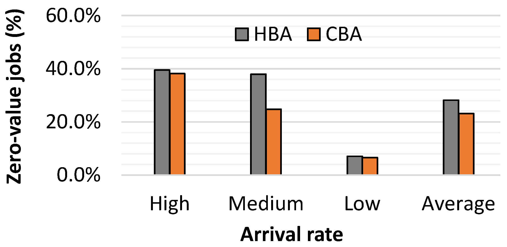
5.1.3. Percentage of Zero-Value Jobs

This metric is important as it relates to user satisfaction with the system: more jobs successfully serviced implies more users serviced and therefore more satisfied users. Figure 6 shows the percentage of zero-value jobs for both approaches at each of the different arrival rates. The average over each of the different arrival rates is also shown. Note that the rejections of jobs were implicit in the maximum reward check, they were not actually removed from the queue though it would be possible to add that functionality. It can be observed that, for all arrival rates, CBA had a lower percentage of zero-value jobs. This was less significant at the high and low arrival rates. For the high arrival rate, this was due to such a large number of jobs arriving that it was impossible to service a large number of them regardless of approach. For the low arrival rate, the difference was again likely due to the exploration part of the algorithm. The initial exploration caused a number of early jobs to be executed after the deadline while the algorithm learned the initial average reward for each possible allocation. The effect of exploration based on uncertainty after initial exploration was unlikely to have much effect on the number of jobs which give zero-value as this exploration favored jobs with reasonably high expected value already. On average, CBA provided 5% more user satisfaction than that of HBA.

5.1.4. Overhead Analysis

Computational complexity of CBA was no higher than the heuristic algorithm HBA. It did perform slightly more mathematical operations per iteration, but it was the same number of iterations required. The average time to find the allocation for a job by CBA was 0.12 milliseconds and the average energy consumption for it was 0.3 millijoules, which was quite low.
Memory overhead of CBA as compared to HBA was negligibly higher as it stored only a few extra numbers per job.
These overheads both in terms of timing and energy consumption were part of the overall profit and energy consumption results, which were better by CBA over HBA. Next, we will discuss the results related to BCC algorithm.

5.2. Experimental Results for BCC Algorithm

In this section, we discuss modeling, results and the corresponding analysis of the proposed server consolidation method. We first estimate the power reduction from proposed BCC server consolidation algorithm for both wired and wireless networks. Next, we evaluate the network-level performance with the consolidation algorithm in an HPC data center with network-level simulations. Before presenting and analyzing the results we describe the data center traffic generation procedure and simulation platform in the next subsections.

5.2.1. Traffic Generation and Simulation Platform for BCC

The BCC algorithm was evaluated with a set of traffic flows based on application demands. Real data center traffic for typical query/search type applications like map-reduce and index-search were measured in [43]. Using these measured traffic flows, a Poisson shot-noise based model to synthesize data center traffic was proposed and verified in [42]. According to [42], the new flow arrival time, the flow duration and the injection rate for each application followed a Poisson, Pareto and, Gaussian distribution respectively. The new flow arrival time was generated using a Poisson distribution with an average flow arrival rate. The average flow arrival rate was considered to be 1000 flows/s for the small-sized DCN [43]. In our evaluations, we considered a Gaussian distribution for the injection rate to have a mean of 8.0 Kbps as the base case for the simulation. Application flow duration was generated following an independent Pareto distribution having a minimum duration of 10 microseconds [43] and a mean of 1 s. We then increased the average injection rates on an incremental basis to 8 Mbps, 100 Mbps, 400 Mbps, and 650 Mbps and regenerated new traffic which represented different types of multimedia traffic and repeat the simulations. We used the Network Simulator-3 (NS-3) suite [49] to evaluate the performance of BCC for both wired fat-tree and wireless S2S-WiDCN networks. NS-3 supported the characteristics of wireless propagation as well as network-level communications. This simulation platform was used to evaluate the S2S-WiDCN with and without consolidation and compare it with the fat-tree wired DCN. For the fat-tree based wired data center architecture, we considered 1.0 Gbps links between servers to access switches and 40.0 Gbps upper-layer links. For all the cases, the migration cost for consolidation is not included in the performance analysis. We have compared the performance of the BCC consolidation algorithm for S2S-WiDCN with traditional wired fat-tree based DCN. We considered a small data center consisting of 800 servers arranged in a 20 × 8 array of racks as [25]. Each of the racks housed five servers and occupied an area of 0.6 m × 0.9 m and is 2 m high. There were 10 racks arranged in a single row and two columns of 8 rows, totaling 160 racks. In our simulations, the racks were assumed to be without any front or back door. In the traditional wired fat-tree based DCN, we considered the same number of servers arranged in same layout as S2S-WiDCN. We considered three hierarchical network layers consisting of 160 access, two aggregate, and two core layer switches, where each rack having an access layer switch.

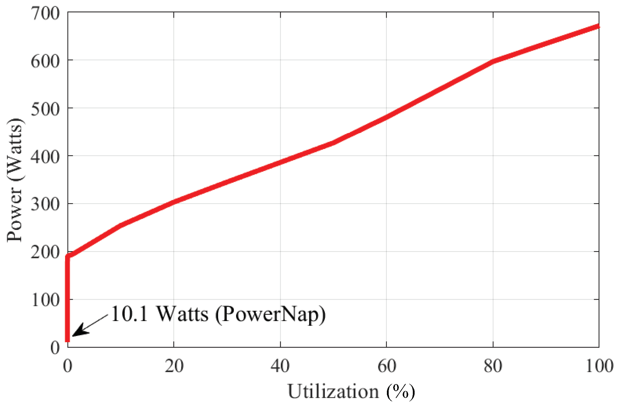
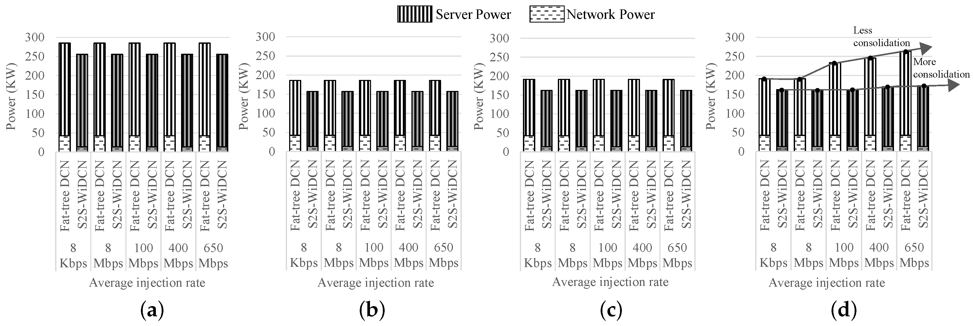
5.2.2. Power Consumption Analysis of BCC

Here we discuss the model and parameters used in power estimation followed by the results.
Power Model for BCC:
It was not a straightforward task to estimate the actual electrical power consumed by an HPC data center. The power consumption depended on several internal factors such as utilization of computing power, the cooling mechanism, and data center networks. Data center power consumption was also affected by external parameters like the geographical location, weather, temperature, and humidity. The total IT power consumption of a data center, P I T consisted of power consumption of the servers ( P S e r v e r ) and network component ( P N e t w o r k ) of the HPC data center. Hence,
P I T = P S e r v e r s + P N e t w o r k
A major portion of P I T comes from P S e r v e r s [50,51]. However, the power consumption of servers varies significantly with the change in CPU utilization [45]. If the utilization of i-th server is denoted by u i , the Power consumption of that server can be given by P S e r v e r ( u i ) , where the dependence of server power on utilization is adopted from [52]. Hence, Equation (21) can be rewritten as:
P I T = i = 1 N P s e r v e r ( u i ) + P n e t w o r k
For the power analysis, we used the power profile of Dell Inc. PowerEdge C5220 (Intel Xeon E3-1265LV2) servers. Power consumption at different server utilization was modeled from the measurement done by the Standard Performance Evaluation Corporation’s S P E C p o w e r _ s s j 2008 database for the same server [52]. In addition to the above power model for the server, we considered an idle server to be placed in the PowerNap state [45] with minimal power consumption. The power profile of a server against different utilization is shown in Figure 7. Although compared to the server power, the power consumption of the network of an HPC data center was small, but it was not negligible [50]. One of the issues with the networking equipment was that they needed to be turned on all the time. The static power portion of the networking equipment dominated the total power consumed by the network [53]. In [53], it was shown that for a network switch, only 8% power reduced during full load to no load transition. Moreover, for the wired network, upper-level switches experienced a similar amount of traffic before and after the consolidation as the majority of the flows remained inside of the rack. For this reason, we neglected the change in networking power equipment due to the variation in injection rate or throughput. We estimated power consumption for wired DCNs using commercially available data from Cisco network switches [54] and Silicom network interface cards (NIC) [55]. The power consumption of each device used in the network is shown in the Table 2. The total network power is:
P N e t w o r k = N C o r e P C o r e + N A g g P A g g + N A c c P A c c + N P N I C ,
where N C o r e , N A g g , N A c c , N are the number of cores, aggregation, access switches, and the total number of servers, respectively; P C o r e , P A g g , P A c c , P N I C are the power consumption of an individual core, aggregation, access switches, and network interface cards, respectively. In S2S-WiDCN, however, no core, aggregate or access layer switches were needed, but only antennas, transceivers and NICs were required for wireless communication. The power consumption of the wireless 60 GHz transceiver was modeled based upon the assessment of 60 GHz transceivers [56]. The NICs of S2S-WiDCN were equipped with transceivers for horizontal and vertical communication. In the traditional DCN, external connections were established via the two Cisco 7702 switches. To provide equivalent connectivity in S2S-WiDCN, we employed two servers to work as gateways, and their power consumption was modeled as that of the Cisco 7702 switch. The power consumption for communication per server in S2S-WiDCN was calculated as:
P W i r e l e s s = 7 P 60 G H z T r a n + P W i f i C n t r l + P N I C ,
where P 60 G H z T r a n is the power consumption of a single 60 GHz transceiver required for each of the six sectors and the horizontal link and P W i f i C n t r l is the power consumption of the IEEE802.11 2.4/5 GHz ISM adapter for the control channel. Finally, the total power consumption in S2S-WiDCN was:
P N e t w o r k ( W i D C N ) = N C o r e P C o r e + N . P W i r e l e s s .
Comparative Analysis of Power Consumption for BCC:
The IT power consumption of wired and S2S-WiDCN data centers with different consolidation methods including the BCC algorithm with variation in the flow injection rate are shown in Figure 8. These power consumption are computed based on the power model described in the previous sub-section for each of the simulation cases ran in the NS-3 simulator for different consolidation algorithm. In [45], it is observed that the majority of the utilization factor of a server is within the range of 20–30%. Here we adopted the utilization of the server capacity of each server without any consolidation from [45]. Figure 8a represents the power consumption of the HPC data center with no consolidation normal condition (NC) while Figure 8d represents BCC. The figure also contains the power consumption pattern if Clustered Exhaustive Search (CES) algorithm was adopted instead of BCC in Figure 8b. CES is a variant of the BCC algorithm, which finds the optimal migration within each cluster using the exhaustive search, hence being much more computationally expensive. For the sake of comparison, we also simulated a network-unaware greedy approach based consolidation (GRD) which is a variant of NICE [11] and the power consumption pattern is shown in Figure 8c. For both wired and wireless networks, at lower injection rates, all the consolidation techniques performed similarly and resulted in significant power consumption reduction compared to NC, while CES consumed the least power. BCC algorithm consumed only 2.83% more power than CES, whereas CES was significantly more computationally complex than BCC because of exhaustive search as discussed in Section 4.4. Hence during the consolidation operation, for moderate to large size of data centers, CES algorithm became impractical to implement as it was not able to perform real-time operations, whereas the BCC algorithm could. BCC algorithm for S2S-WiDCN reduced 37% power consumption compared to the NC case.
For higher injection rates, CES and GRD consumed significantly less server power compared to BCC for wired networks. This was because the CES and GRD did not consider the network bandwidth constraints while consolidating, resulting in more aggressive consolidation that in the BCC. Therefore, this difference became more apparent with increase in flow injection rates. However, this reduction of power came at the cost of the lower throughput because the CES and GRD algorithms did not consider the network traffic characteristics. This impact on performance will be discussed in detail in Section 5.2.3. Moreover, the computational complexity of CES was orders of magnitude higher than the BCC.
For BCC consolidation in S2S-WiDCN, similar to the wired network, with the increase in flow injection rate, the server power consumption increased, while for CES and GRD power consumption remained the same. Hence, at higher injection rate, CES and GRD consumed less power compared to BCC. However, this reduction of power came at the cost of lower throughput as CES and GRD algorithms did not consider the network traffic characteristics while consolidating. However, the increase in power consumption in BCC for S2S-WiDCN was not as drastic as in the case of wired data center. This is demonstrated by the trend arrows in Figure 8d. This was because, in the S2S-WiDCN architecture, a server had the potential to sustain a maximum of seven simultaneous links at a time with other servers in its vertical plane and horizontal line. On the contrary, in the wired architecture, there existed only one link per server albeit, of higher bandwidth. As a result, for the wired DCN with BCC, many of the VM migration attempts failed due to the violation of the inequality of (5) compared to the S2S-WiDCN. This suggested that the bandwidth constrained network-aware consolidation, BCC, was more effective on S2S-WiDCN.

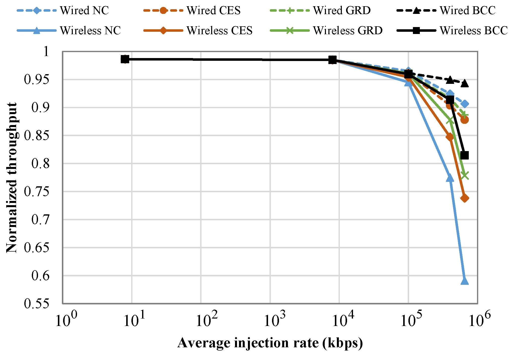
5.2.3. Performance Analysis of BCC

Here we present the network-level performance of the S2S-WiDCN with BCC along with a comparative analysis with respect to wired fat-tree DCNs in terms of throughput.
The throughput was defined as the average rate of bit transferred per second over the DCN. The normalized throughput of both S2S-WiDCN and fat-tree architecture for different injection rates at NC, CES, GRD and BCC consolidation are shown in Figure 9. Normalized throughput was defined as the ratio of the average throughput achieved and average injection rate. For NC, although it was seen that for lower injection rate both S2S-WiDCN and fat-tree network showed similar throughput, but for both the networks, the achieved throughput started to decrease as the average injection rate went beyond 100 Mbps. However, degradation was different for wired and wireless DCNs. The throughput reduced more for the wireless DCN than the wired counterpart for higher injection rates due to the lower physical bandwidth available per channel for the wireless links of 0.563 Gbps compared to 1.0 Gbps for the wires. Further, from Figure 9, it can be seen that, for the lower injection rates, there was no significant difference in achieved throughput with BCC consolidation for both wired and wireless data centers. These throughputs were also similar compared to that NC case. However, for higher injection rates beyond 100 Mbps, for both S2S-WiDCN and fat-tree network, achieved throughput increased compared to the NC. The main contributing factor was that, due to the VM migrations, in many cases, both source and destination of flows ended up in the same physical server. Therefore, these flows are effectively eliminated from the network, which ultimately increased the average throughput of the entire network compared to NC. On the other hand, instead of BCC, if CES or GRD consolidation was implemented, at lower injection rates, there was no significant difference in achieved throughput for both S2S-WiDCN and fat-tree networks compared to BCC. For the higher injection rates beyond 100 Mbps, the performance of the wireless networks improved compared to NC, but not as well as BCC. However, the performance of the wired network degraded with the incorporation of CES or GRD consolidation algorithm. This contrasting behavior was mainly due to the number of channels available in different architectures. Due to all flows in the wired data center being channelized over the same link, the aggregate flow rate after CES or GED exceeded the physical link bandwidth violating (5). This caused degradation in throughput. On the contrary, in the S2S-WiDCN, due to the presence of multiple vertical sectors and the horizontal link a relatively larger number of flows did not violate (5) resulting in better performance compared to the wired data center.

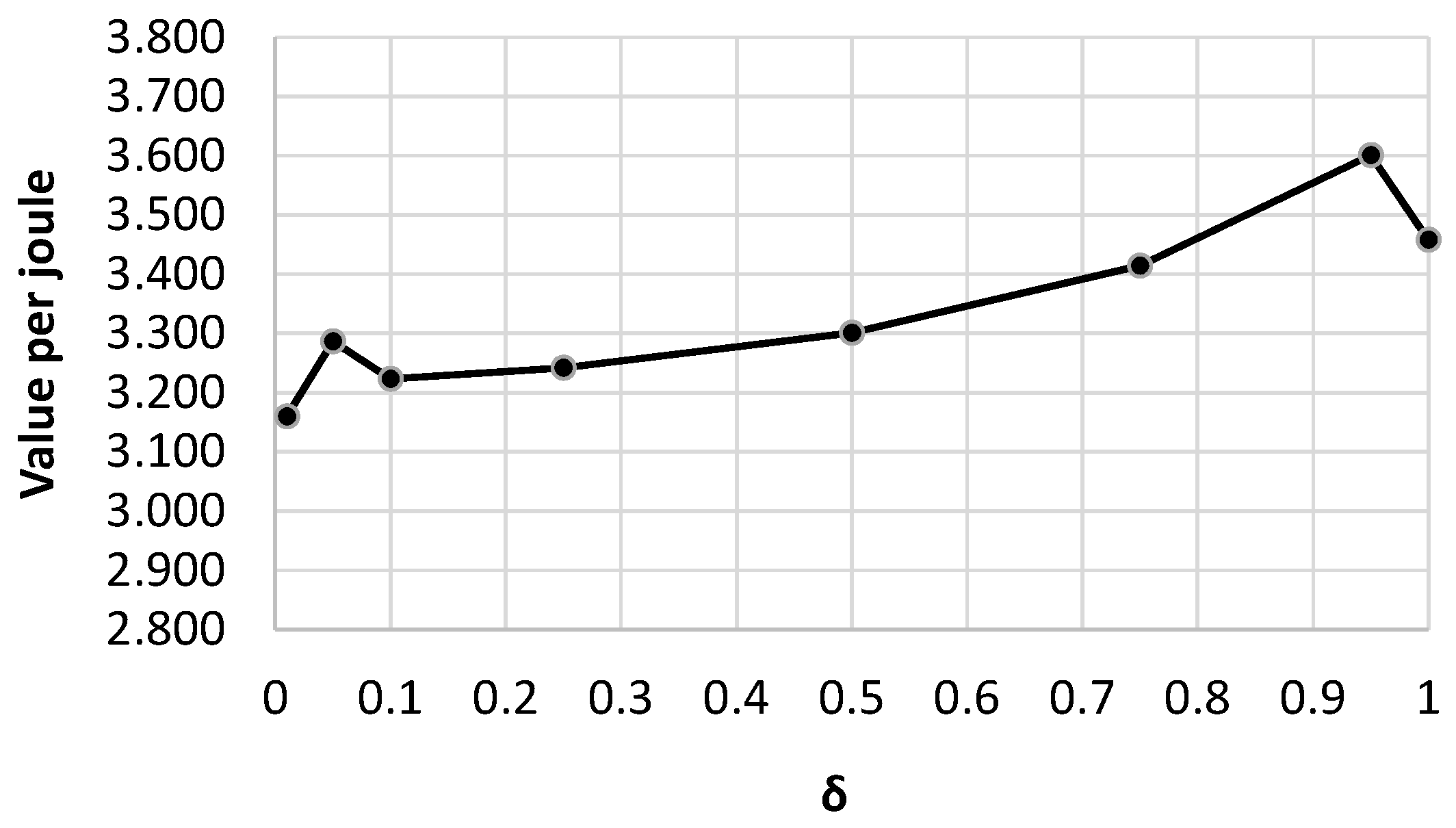
5.2.4. Accuracy of Inter-Consolidation Time Modeling

In this section, the inter-consolidation time for the BCC algorithm is analyzed and the accuracy of the mathematical estimation of inter-consolidation time is evaluated. The expected inter consolidation cost estimated from (15) is shown in Figure 10 for a data center consisting of 800 servers as discussed in Section 5.2.1.
To verify the mathematical model for cost of consolidation (15), we ran a Monte Carlo simulation for each ρ 300 times and calculated the value of the cost function. For these cases, the values for η 1 , ν , κ considered here were 200, 1000, and 1 respectively. The average size of migration ν was considered as 1000 Megabytes which represents a practical value. For η 1 , we ran the server consolidation simulation for different random initial conditions for thousands of times and used the average number of idle servers in PowerNap mode after the first cycle of server migration. We considered κ = 1 to put equal emphasis on power saving and network performance on the cost. Nevertheless, these values needed not necessarily be exactly the same across all the data centers. Depending on the capacity, performance requirements and physical limitations, these values could vary for different HPC data centers.
The average of the simulated values from the different run for each ρ are shown in Figure 10. The cost estimates in this method relied on many repetitive simulations and were highly computationally expensive as each of simulation at a particular ρ and t was repeated at least 1000 times to find the expected cost using Monte-Carlo method. On the contrary, using (15) the cost and optimal inter-consolidation time could be approximated much faster. The optimal inter-consolidation time for different ρ identified from both methods is shown in Figure 11. It was observed that for lower values of ρ ( ρ 0.55 ), the optimal inter-consolidation time estimated from the mathematical equation closely approximated the measured value from the Monte Carlo simulation. On the contrary, for higher values of ρ , the optimal inter-consolidation time estimated from the mathematical analysis deviated from the value measured through simulations. However, at higher ρ , the absolute value of the cost was less sensitive to the inter-consolidation time. This shows that although at higher ρ the inter-consolidation time suggested by the model may deviate from the actual optimal interval, the actual cost incurred at this non-optimal interval was not much different compared to that at the optimal interval. Hence the optimal inter-consolidation time could be estimated reasonably accurately from the mathematical form.
We used MATLAB R2018b on a system having Intel Core i7 with 16 GB memory to calculate the inter consolidation time with both Monte-Carlo simulation and mathematical model. On average, computation time required for the Monte-Carlo simulation took 1039.4 s to complete the calculation while the mathematical model took only about 0.798 s on average. Hence there was more than 1000× speedup in calculation time using the mathematical model.

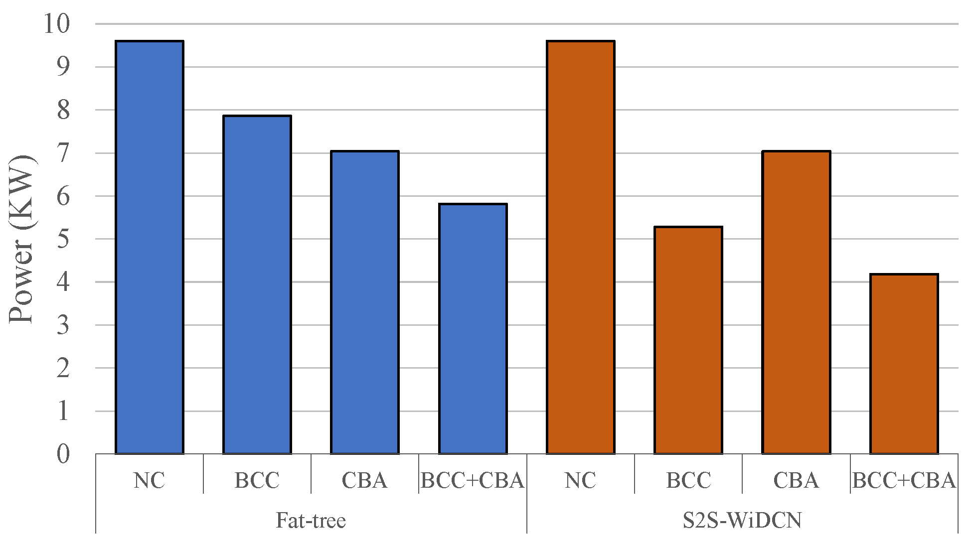
5.3. Overall Power Saving with a Combination of BCC and CBA

In this subsection we discuss the combined effect of CBA and BCC together for power saving. We evaluated the power consumption of a data center consisting of 800 servers with a higher injection rate traffic having an average flow rate of 400 Mbps. For this comparison, the power consumption of each server was modeled based on Odroid-XU3 board. The power consumption of the Odroid-XU3 at PowerNap was conservatively assumed to be 1 watt and the full load power consumption was 20 Watts. We also assumed that the power saving ratio per device followed the energy saving ratio due to CBA algorithm. In Figure 12 we showed the power consumption of the data center in different cases including, normal condition (NC), utilizing BCC only, utilizing CBA only and finally, utilizing both BCC and CBA together.
At higher datarate, BCC consolidation could reduce the power consumption of the overall data center more for S2S-WiDCN compared to fat-tree network. The CBA algorithm working standalone outperformed BCC for fat-tree wired network while in S2S-WiDCN, BCC could reduce more power compared to CBA. Nevertheless, for both wired and wireless networks, combining both BCC and CBA could achieve maximum power reduction.

6. Conclusions

In this paper we investigated an algorithm for jointly optimizing value and energy when considering resource allocation in HPC data centers. The algorithm was created under the assumption that no prior information is available for accurate predictions of job value and energy, instead it used a technique inspired by reinforcement learning to explore the value and energy of jobs before exploiting in future allocations. It has also been shown that the percentage of zero-value jobs is lower for all of the different arrival rates for CBA. We have also incorporated a server consolidation algorithm BCC for both wired and wireless data center networks. We have shown that both the approaches significantly reduce energy and power consumption of the entire data center. It has been observed that, if BCC and CBA are adopted simultaneously for the wireless HPC data center architecture, maximum power saving can be achieved. We also derived a mathematical model for BCC for determining optimal inter-consolidation interval to enable the data center resource management unit to schedule consolidations at optimal intervals without relying on computationally expensive simulations to estimate the optimal interval.

Author Contributions

Conceptualization, A.K.S., A.G. (Amlan Ganguly), G.V.M. and B.M.A.-H.; Data curation, S.A.M. and A.G. (Alexander Gilday); Formal analysis, S.A.M. and A.G. (Alexander Gilday); Investigation, S.A.M., A.G. (Alexander Gilday), A.K.S., A.G. (Amlan Ganguly) and X.W.; Methodology, X.W.; Supervision, A.K.S., A.G. (Amlan Ganguly), G.V.M. and B.M.A.-H.; Writing—original draft, S.A.M. and A.G. (Alexander Gilday); Writing—review & editing, S.A.M. and A.G. (Alexander Gilday). All authors have read and agreed to the published version of the manuscript.

Funding

This work was supported in part by the Engineering and Physical Sciences Research Council under EPSRC Grant EP/L000563/1, and EP/K034448/1 the PRiME Programme Grant (www.prime-project.org), and US National Science Foundation(NSF) CAREER grant CNS-1553264.

Conflicts of Interest

The authors declare no conflict of interest.

References

  1. Rodero, I.; Jaramillo, J.; Quiroz, A.; Parashar, M.; Guim, F.; Poole, S. Energy-efficient application-aware online provisioning for virtualized clouds and data centers. In Proceedings of the International Green Computing Conference (IGCC), Chicago, IL, USA, 15–18 August 2010; pp. 31–45. [Google Scholar] [CrossRef]
  2. Benini, L.; Micheli, G.d. System-level power optimization: Techniques and tools. ACM Trans. Des. Autom. Electron. Syst. (Todaes) 2000, 5, 115–192. [Google Scholar] [CrossRef] [Green Version]
  3. Aksanli, B.; Rosing, T. Providing regulation services and managing data center peak power budgets. In Proceedings of the 2014 Design, Automation & Test in Europe Conference & Exhibition (DATE), Dresden, Germany, 24–28 March 2014; pp. 143–147. [Google Scholar]
  4. Bogdan, P.; Garg, S.; Ogras, U.Y. Energy-efficient computing from systems-on-chip to micro-server and data centers. In Proceedings of the 2015 Sixth International Green Computing Conference and Sustainable Computing Conference (IGSC), Las Vegas, NV, USA, 14–16 December 2015; pp. 1–6. [Google Scholar]
  5. Koomey, J. Growth in data center electricity use 2005 to 2010. In A Report by Analytical Press, Completed at the Request of The New York Times; Analytics Press: Burlingame, CA, USA, 2011. [Google Scholar]
  6. Verma, A.; Ahuja, P.; Neogi, A. pMapper: Power and migration cost aware application placement in virtualized systems. In Proceedings of the 9th ACM/IFIP/USENIX International Conference on Middleware, Leuven, Belgium, 1–5 December 2008; pp. 243–264. [Google Scholar]
  7. Jung, G.; Hiltunen, M.A.; Joshi, K.R.; Schlichting, R.D.; Pu, C. Mistral: Dynamically managing power, performance, and adaptation cost in cloud infrastructures. In Proceedings of the 2010 IEEE 30th International Conference on Distributed Computing Systems, Genova, Italy, 21–25 June 2010; pp. 62–73. [Google Scholar]
  8. Zu, Y.; Huang, T.; Zhu, Y. An efficient power-aware resource scheduling strategy in virtualized datacenters. In Proceedings of the IEEE 2013 International Conference on Parallel and Distributed Systems, Seoul, Korea, 15–18 December 2013; pp. 110–117. [Google Scholar]
  9. Mann, V.; Kumar, A.; Dutta, P.; Kalyanaraman, S. VMFlow: Leveraging VM mobility to reduce network power costs in data centers. In International Conference on Research in Networking; Springer: New York, NY, USA, 2011; pp. 198–211. [Google Scholar]
  10. Huang, D.; Yang, D.; Zhang, H.; Wu, L. Energy-aware virtual machine placement in data centers. In Proceedings of the 2012 IEEE Global Communications Conference (GLOBECOM), Anaheim, CA, USA, 3–7 December 2012; pp. 3243–3249. [Google Scholar]
  11. Cao, B.; Gao, X.; Chen, G.; Jin, Y. NICE: Network-aware VM consolidation scheme for energy conservation in data centers. In Proceedings of the 2014 20th IEEE International Conference on Parallel and Distributed Systems (ICPADS), Hsinchu, Taiwan, 16–19 December 2014; pp. 166–173. [Google Scholar]
  12. Ferreto, T.C.; Netto, M.A.; Calheiros, R.N.; De Rose, C.A. Server consolidation with migration control for virtualized data centers. Future Gener. Comput. Syst. 2011, 27, 1027–1034. [Google Scholar] [CrossRef]
  13. Sun, G.; Liao, D.; Zhao, D.; Xu, Z.; Yu, H. Live migration for multiple correlated virtual machines in cloud-based data centers. IEEE Trans. Serv. Comput. 2015, 11, 279–291. [Google Scholar] [CrossRef]
  14. Kliazovich, D.; Bouvry, P.; Khan, S.U. DENS: Data center energy-efficient network-aware scheduling. Clust. Comput. 2013, 16, 65–75. [Google Scholar] [CrossRef]
  15. Khemka, B.; Friese, R.; Pasricha, S.; Maciejewski, A.A.; Siegel, H.J.; Koenig, G.A.; Powers, S.; Hilton, M.; Rambharos, R.; Poole, S. Utility maximizing dynamic resource management in an oversubscribed energy-constrained heterogeneous computing system. Sustain. Comput. Inform. Syst. 2015, 5, 14–30. [Google Scholar] [CrossRef]
  16. Kim, S.; Kim, Y. Application-specific cloud provisioning model using job profiles analysis. In Proceedings of the 2012 IEEE 14th International Conference on High Performance Computing and Communication & 2012 IEEE 9th International Conference on Embedded Software and Systems (HPCC-ICESS), Liverpool, UK, 25–27 June 2012; pp. 360–366. [Google Scholar]
  17. Singh, A.K.; Dziurzanski, P.; Indrusiak, L.S. Value and energy optimizing dynamic resource allocation in many-core HPC systems. In Proceedings of the 2015 IEEE 7th International Conference on Cloud Computing Technology and Science (CloudCom), Vancouver, BC, Canada, 30 November–3 December 2015; pp. 180–185. [Google Scholar]
  18. Baccour, E.; Foufou, S.; Hamila, R.; Hamdi, M. A survey of wireless data center networks. In Proceedings of the 2015 49th Annual Conference on Information Sciences and Systems (CISS), Vancouver, BC, Canada, 30 November–3 December 2015; pp. 1–6. [Google Scholar]
  19. Vardhan, H.; Ryu, S.R.; Banerjee, B.; Prakash, R. 60 GHz wireless links in data center networks. Comput. Netw. 2014, 58, 192–205. [Google Scholar] [CrossRef]
  20. Halperin, D.; Kandula, S.; Padhye, J.; Bahl, P.; Wetherall, D. Augmenting data center networks with multi-gigabit wireless links. ACM Sigcomm Comput. Commun. Rev. 2011, 41, 38–49. [Google Scholar] [CrossRef]
  21. Zaaimia, M.; Touhami, R.; Fono, V.; Talbi, L.; Nedil, M. 60 GHz wireless data center channel measurements: Initial results. In Proceedings of the 2014 IEEE International Conference on Ultra-WideBand (ICUWB), Paris, France, 1–3 September 2014; pp. 57–61. [Google Scholar]
  22. Mamun, S.A.; Umamaheswaran, S.G.; Chandrasekaran, S.S.; Shamim, M.S.; Ganguly, A.; Kwon, M. An Energy-Efficient, Wireless Top-of-Rack to Top-of-Rack Datacenter Network Using 60 GHz Links. In Proceedings of the 2017 IEEE Green Computing and Communications (GreenCom), Exeter, UK, 21–23 June 2017; pp. 458–465. [Google Scholar]
  23. Cheng, C.L.; Zajić, A. Characterization of 300 GHz Wireless Channels for Rack-to-Rack Communications in Data Centers. In Proceedings of the 2018 IEEE 29th Annual International Symposium on Personal, Indoor and Mobile Radio Communications (PIMRC), Bologna, Italy, 9–12 September 2018; pp. 194–198. [Google Scholar]
  24. Shin, J.Y.; Kirovski, D.; Harper, D.T., III. Data Center Using Wireless Communication. U.S. Patent 9,391,716, 12 July 2016. [Google Scholar]
  25. Mamun, S.A.; Umamaheswaran, S.G.; Ganguly, A.; Kwon, M.; Kwasinski, A. Performance Evaluation of a Power-Efficient and Robust 60 GHz Wireless Server-to-Server Datacenter Network. IEEE Trans. Green Commun. Netw. 2018, 2, 1174–1185. [Google Scholar] [CrossRef]
  26. Auer, P. Using confidence bounds for exploitation-exploration trade-offs. J. Mach. Learn. Res. 2002, 3, 397–422. [Google Scholar]
  27. Yeo, C.S.; Buyya, R. A Taxonomy of Market-based Resource Management Systems for Utility-driven Cluster Computing. Softw. Pract. Exp. 2006, 36, 1381–1419. [Google Scholar] [CrossRef]
  28. Theocharides, T.; Michael, M.K.; Polycarpou, M.; Dingankar, A. Hardware-enabled Dynamic Resource Allocation for Manycore Systems Using Bidding-based System Feedback. EURASIP J. Embed. Syst. 2010, 2010, 261434. [Google Scholar] [CrossRef] [Green Version]
  29. Locke, C.D. Best-Effort Decision-Making for Real-Time Scheduling. Ph.D. Thesis, Carnegie Mellon University, Pittsburgh, PA, USA, 1986. [Google Scholar]
  30. Aldarmi, S.; Burns, A. Dynamic value-density for scheduling real-time systems. In Proceedings of the Euromicro Conference on Real-Time Systems, York, UK, 9–11 June 1999; pp. 270–277. [Google Scholar]
  31. Bansal, N.; Pruhs, K.R. Server Scheduling to Balance Priorities, Fairness, and Average Quality of Service. SIAM J. Comput. 2010, 39, 3311–3335. [Google Scholar] [CrossRef] [Green Version]
  32. Hussin, M.; Lee, Y.C.; Zomaya, A.Y. Efficient energy management using adaptive reinforcement learning-based scheduling in large-scale distributed systems. In Proceedings of the 2011 International Conference on Parallel Processing, Taipei, Taiwan, 13–16 September 2011; pp. 385–393. [Google Scholar]
  33. Lin, X.; Wang, Y.; Pedram, M. A reinforcement learning-based power management framework for green computing data centers. In Proceedings of the 2016 IEEE International Conference on Cloud Engineering (IC2E), Berlin, Germany, 4–8 April 2016; pp. 135–138. [Google Scholar]
  34. Singh, A.K.; Dziurzanski, P.; Indrusiak, L.S. Value and energy aware adaptive resource allocation of soft real-time jobs on many-core HPC data centers. In Proceedings of the 2016 IEEE 19th International Symposium on Real-Time Distributed Computing (ISORC), York, UK, 17–20 May 2016; pp. 190–197. [Google Scholar]
  35. Sun, X.; Ansari, N.; Wang, R. Optimizing resource utilization of a data center. IEEE Commun. Surv. Tutor. 2016, 18, 2822–2846. [Google Scholar] [CrossRef]
  36. Ray, M.; Sondur, S.; Biswas, J.; Pal, A.; Kant, K. Opportunistic power savings with coordinated control in data center networks. In Proceedings of the 19th International Conference on Distributed Computing and Networking, Varanasi, India, 4–7 January 2018; p. 48. [Google Scholar]
  37. Farrington, N.; Porter, G.; Radhakrishnan, S.; Bazzaz, H.H.; Subramanya, V.; Fainman, Y.; Papen, G.; Vahdat, A. Helios: A hybrid electrical/optical switch architecture for modular data centers. ACM SIGCOMM Comput. Commun. Rev. 2011, 41, 339–350. [Google Scholar]
  38. Calheiros, R.N.; Buyya, R. Energy-Efficient Scheduling of Urgent Bag-of-Tasks Applications in Clouds Through DVFS. In Proceedings of the IEEE International Conference on Cloud Computing Technology and Science (CLOUDCOM), Singapore, 15–18 December 2014; pp. 342–349. [Google Scholar]
  39. Irwin, D.E.; Grit, L.E.; Chase, J.S. Balancing Risk and Reward in a Market-Based Task Service. In Proceedings of the IEEE International Symposium on High Performance Distributed Computing (HPDC), Honolulu, HI, USA, 4–6 June 2004; pp. 160–169. [Google Scholar]
  40. Bubeck, S.; Cesa-Bianchi, N. Regret analysis of stochastic and nonstochastic multi-armed bandit problems. Found. Trends Mach. Learn. 2012, 5, 1–122. [Google Scholar] [CrossRef] [Green Version]
  41. Carpentier, A.; Lazaric, A.; Ghavamzadeh, M.; Munos, R.; Auer, P. Upper-confidence-bound algorithms for active learning in multi-armed bandits. In International Conference on Algorithmic Learning Theory; Springer: New York, NY, USA, 2011; pp. 189–203. [Google Scholar]
  42. Han, Y.; Yoo, J.H.; Hong, J.W.K. Poisson shot-noise process based flow-level traffic matrix generation for data center networks. In Proceedings of the 2015 IFIP/IEEE International Symposium on Integrated Network Management (IM), Ottawa, ON, Canada, 11–15 May 2015; pp. 450–457. [Google Scholar]
  43. Benson, T.; Akella, A.; Maltz, D.A. Network traffic characteristics of data centers in the wild. In Proceedings of the 10th ACM SIGCOMM Conference on Internet Measurement, Melbourne, Australia, 1–3 November 2010; pp. 267–280. [Google Scholar]
  44. Dutt, S. New faster kernighan-lin-type graph-partitioning algorithms. In Proceedings of the 1993 International Conference on Computer Aided Design (ICCAD), Santa Clara, CA, USA, 7–11 November 1993; pp. 370–377. [Google Scholar]
  45. Meisner, D.; Gold, B.T.; Wenisch, T.F. PowerNap: Eliminating server idle power. ACM SIGARCH Comput. Archit. News 2009, 44, 205–216. [Google Scholar] [CrossRef]
  46. Zhang, J.; Yu, F.R.; Wang, S.; Huang, T.; Liu, Z.; Liu, Y. Load Balancing in Data Center Networks: A Survey. IEEE Commun. Surv. Tutor. 2018, 20, 2324–2352. [Google Scholar] [CrossRef]
  47. Davidson, A.; Tarjan, D.; Garland, M.; Owens, J.D. Efficient parallel merge sort for fixed and variable length keys. In Proceedings of the 2012 Innovative Parallel Computing (InPar), San Jose, CA, USA, 13–14 May 2012; pp. 1–9. [Google Scholar]
  48. Kleinrock, L. Queueing Systems, Volume 2: Computer Applications; Wiley: New York, NY, USA, 1976. [Google Scholar]
  49. ns-3 Network Simuilator. Available online: https://www.nsnam.org/ (accessed on 4 July 2019).
  50. Shehabi, A.; Smith, S.J.; Sartor, D.A.; Brown, R.E.; Herrlin, M.; Koomey, J.G.; Masanet, E.R.; Horner, N.; Azevedo, I.L.; Lintner, W. United States Data Center Energy Usage Report; Technical Report LBNL-1005775; LBNL: Berkeley, CA, USA, 2016.
  51. Pelley, S.; Meisner, D.; Wenisch, T.F.; VanGilder, J.W. Understanding and abstracting total data center power. In Proceedings of the 2009 Workshop on Energy Efficient Design (WEED), Ann Arbor, MI, USA, 20 June 2009. [Google Scholar]
  52. SPECpower_ssj2008. Results for Dell Inc. PowerEdge C5220. Available online: https://www.spec.org/power_ssj2008/results/res2013q2/power_ssj2008-20130402-00601.html (accessed on 4 July 2019).
  53. Heller, B.; Seetharaman, S.; Mahadevan, P.; Yiakoumis, Y.; Sharma, P.; Banerjee, S.; McKeown, N. Elastictree: Saving Energy in Data Center Networks. In Proceedings of the 7th USENIX Conference on Networked Systems Design and Implementation (NSDI), San Jose, CA, USA, 28–30 April 2010; pp. 249–264. [Google Scholar]
  54. Cisco. Cisco Data Center Switches. Available online: https://www.cisco.com/c/en/us/products/switches/data-center-switches/index.html (accessed on 4 July 2019).
  55. Silicom. Silicom PE2G2I35 Datasheet. Available online: http://www.silicom-usa.com/wp-content/uploads/2016/08/PE2G2I35-1G-Server-Adapter.pdf (accessed on 4 July 2019).
  56. Analog Devices. Analog Devices HMC6300 and HMC6301 60 GHz Millimeter Wave Transmitter and Receiver Datasheet. Available online: http://www.analog.com/media/en/technical-documentation/data-sheets/HMC6300.pdf (accessed on 4 July 2019).
Publisher’s Note: MDPI stays neutral with regard to jurisdictional claims in published maps and institutional affiliations.
Figure 1. The model of the system targeted by this paper. A High Performance Computing (HPC) data center containing multiple nodes with many-core CPUs.
Jlpea 10 00032 g001
Figure 2. An example value curve of a job.
Jlpea 10 00032 g002
Figure 3. Timeline of consolidation operations.
Jlpea 10 00032 g003
Figure 4. Value/energy for different confidence values.
Jlpea 10 00032 g004
Figure 5. Value earned and energy consumed at different arrival rates.
Jlpea 10 00032 g005
Figure 6. Percentage of zero-value jobs at various arrival rates.
Jlpea 10 00032 g006
Figure 7. Power profile with varying utilization of PowerEdge C5220 server [52].
Jlpea 10 00032 g007
Figure 8. Power consumption comparison of different architecture for (a) no consolidation (NC) (b) clustered exhaustive search (CES) (c) Greedy approach base consolidation (GRD) and (d) bandwidth constrained consolidation (BCC). The arrows denote the power saving due to BCC.
Jlpea 10 00032 g008
Figure 9. Average throughput for different data center architecture with NC, CES, GRD and BCC consolidation normalized with flow injection rate.
Jlpea 10 00032 g009
Figure 10. Consolidation cost estimated from mathematical analysis (dashed line) and from Monte Carlo simulation (solid line) with respect to inter-consolidation time.
Jlpea 10 00032 g010
Figure 11. Comparison of optimal inter-consolidation time obtained from the mathematical model and Monte-Carlo simulations at different ρ .
Jlpea 10 00032 g011
Figure 12. Power consumption comparison between normal condition, BCC, CBA and combination of BCC and CBA.
Jlpea 10 00032 g012
Table 1. Value at different execution times for PARSEC benchmark applications.
ApplicationExecution Time (s)Value (Currency)
blackscholes4691210080500
bodytrack68111410080500
dedup5791210080500
facesim815182210080500
ferret2226293110080500
fluidanimate79111410080500
freqmine915172010080500
streamcluster2228354210080500
vips911131610080500
Table 2. Power consumption of different data center network (DCN) components.
DeviceModelUsed inPower (W)
Access Layer SwitchCisco 9372Fat-Tree210.0
Aggregate Layer SwitchCisco 9508Fat-Tree2527.0
Core Layer SwitchCisco 7702Fat-Tree, S2S-WiDCN837.0
Network Interface CardSilicom PE2G2I35Fat-Tree, S2S-WiDCN2.64
60 GHz TransceiverAnalog Device HMC 6300/6301S2S-WiDCN1.70
IEEE802.11 2.4/5 GHz AdapterD-link DWA-171S2S-WiDCN0.22

