Article

Machine Learning-Based Prediction of Multi-Year Cumulative Atmospheric Corrosion Loss in Low-Alloy Steels with SHAP Analysis


1
School of Materials Science and Engineering, Yeungnam University, Gyeongsan 38541, Republic of Korea
2
Institute of Materials Technology, Yeungnam University, Gyeongsan 38541, Republic of Korea
*
Authors to whom correspondence should be addressed.
Coatings 2026, 16(4), 488; https://doi.org/10.3390/coatings16040488
Submission received: 25 March 2026 / Revised: 6 April 2026 / Accepted: 15 April 2026 / Published: 17 April 2026

Highlights

What are the main findings?
  • Five ML models were trained on a 600-sample ISO 9223:2012-grounded dataset for cumulative atmospheric corrosion prediction.
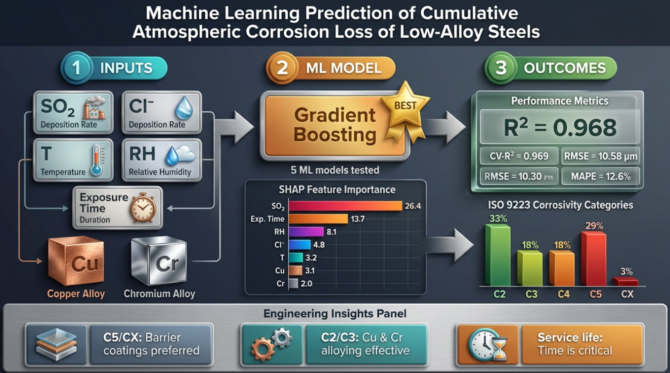
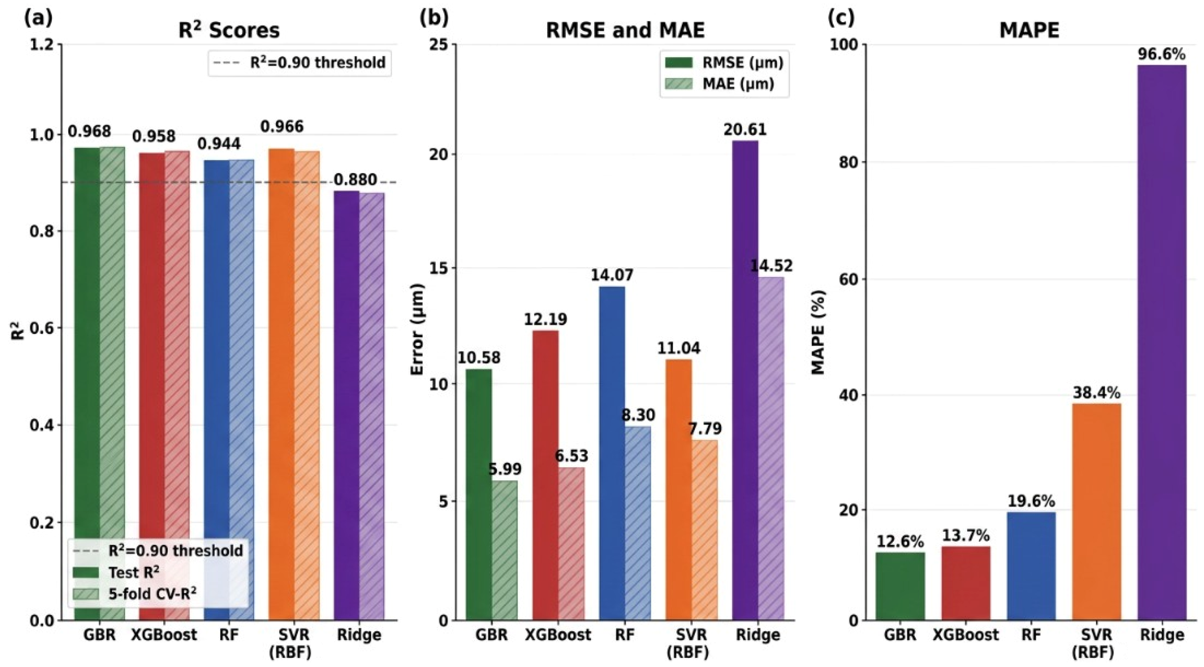
  • Gradient boosting achieves the best accuracy: R2 = 0.968, RMSE = 10.58 µm, and MAPE = 12.6%.
  • XGBoost ranks second (R2 = 0.958), outperforming SVR, random forest, and ridge regression.
  • SHAP analysis identified the SO2 deposition rate, exposure time, and relative humidity as top predictors, which is consistent with ISO 9223 physics.
  • The ISO 9223 corrosivity category hierarchy (CX > C5 > C4 > C3 > C2) was fully validated across the dataset.
What are the implications of the main findings?
  • Multi-year cumulative corrosion loss can be predicted with R2 > 0.96 from 11 environmental and material inputs.
  • Exposure time as an explicit feature is essential for accurate multi-year service-life planning.
  • In C5/CX environments, barrier coatings are critical; in C2/C3 environments, Cu and Cr alloying provides effective protection.
  • SHAP interpretability confirms ML recovers ISO 9223/9224 physics, demonstrating physics-consistency, not just data interpolation.
  • Physics-grounded synthetic datasets enable reproducible ML benchmarks for corrosion science.

Abstract
Atmospheric corrosion of carbon and low-alloy steels causes direct economic losses that are estimated at around 3.4% of the global GDP, and its accurate multi-year prediction is essential for protective coating selection, service-life estimation, and infrastructure maintenance scheduling. In this study, machine learning (ML) algorithms, including gradient boosting regressor (GBR), eXtreme gradient boosting (XGBoost), random forest (RF), support vector regression (SVR), and ridge regression, were trained on a 600-sample physics-grounded dataset to predict the cumulative atmospheric corrosion loss (µm) of low-alloy steels over 1–10 years of exposure. The dataset was constructed using the exact ISO 9223:2012 dose–response function (DRF) for a first-year corrosion rate and the ISO 9224:2012 power-law multi-year kinetic model (C(t) = C1·t0.5), spanning ISO 9223 corrosivity categories C2–CX across 11 environmental and material input features. All models were evaluated on the original (untransformed) corrosion scale under an 80/20 train/test split and five-fold cross-validation. Gradient boosting achieved the best overall performance with test set R2 = 0.968, CV-R2 = 0.969, RMSE = 10.58 µm, MAE = 5.99 µm, and MAPE = 12.6%. XGBoost was a close second (R2 = 0.958, CV-R2 = 0.960). RF achieved an R2 of 0.944. SHAP (SHapley Additive exPlanations) analysis identified SO2 deposition rate, exposure time, relative humidity, Cl deposition rate, and temperature as the five most influential predictors. The dominance of the SO2 deposition rate (mean |SHAP| = 26.37 µm) and the high second-place ranking of exposure time (13.67 µm) are fully consistent with the ISO 9223:2012 dose–response function and ISO 9224:2012 power-law kinetics, respectively, while among the material features, Cu and Cr contents showed the strongest negative SHAP contributions, confirming their corrosion-inhibiting roles in weathering steels. These results establish a physics-consistent, interpretable ML benchmark exceeding R2 = 0.90 for multi-year cumulative corrosion loss prediction and provide a quantitative tool for alloy screening, coating selection in aggressive atmospheric environments, and service-life planning.

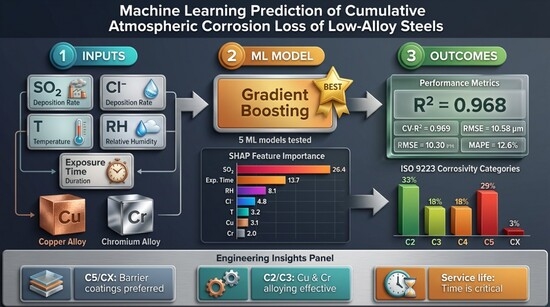
Graphical Abstract

1. Introduction

Atmospheric corrosion of metallic structures represents the most economically significant form of material degradation globally. The direct cost of corrosion across all industrial sectors exceeds ~USD 2.5 trillion per year, which is approximately 3.4% of the global gross domestic product (GDP), with low-alloy steel infrastructure accounting for the largest share [1,2]. Protective coatings are the primary mitigation strategy against atmospheric attack, and the accurate prediction of cumulative corrosion loss over multi-year service lifetimes is a prerequisite for rational protective coating selection, alloy design, and maintenance cost optimization [3,4,5,6]. Conventional protective coating selection for structures in corrosive environments (ISO 9223 categories C3–CX) relies heavily on empirical experience and short-term corrosion data; however, ML-based predictive models that integrate environmental exposure and alloy composition could significantly improve this process [7,8,9].
The rate of atmospheric corrosion is governed by a complex, nonlinear interplay of environmental factors, including temperature (T), relative humidity (RH), SO2 deposition rate (Pd), and Cl deposition rate (Sd), as well as the material composition of the steel. The ISO 9223:2012 standard encodes these relationships through a dose–response function (DRF) that predicts the first-year corrosion rate as a function of four environmental variables [10]. Multi-year cumulative corrosion loss follows the ISO 9224:2012 power-law kinetic model C(t) = C1·tb, where b ≈ 0.5 for carbon steel in most atmospheric environments [11]. While these physics-based models are widely used for corrosivity classification and coating specification, they do not account for material composition effects, nonlinear feature interactions, or the full diversity of real-world atmospheric environments [12]. Machine learning offers a powerful complement to ISO-based models by learning complex input–output relationships from data [13].
ML-based atmospheric corrosion prediction has grown rapidly. Yan et al. [14] used ML algorithms for marine atmospheric corrosion of low-alloy steels and demonstrated that gradient boosting decision trees (GBDT) and XGBoost significantly outperform linear regression, achieving RF training R2 = 0.94 with Cu, Cr, Ni, P, and Si composition and environmental variables as features. Kuang and Long [15] applied six ML algorithms, including XGBoost (best performer), RF, GBDT, and SVR, to low-alloy steel atmospheric corrosion data, identifying Cl deposition rate, SO2 deposition rate, and relative humidity as the most influential predictors. Zhi et al. [16] developed an improved RF model for outdoor atmospheric corrosion with systematic key-factor identification. Li et al. [17] applied ML to ACM sensor data at six atmospheric sites across China, demonstrating the dominance of Cl deposition, time of wetness (TOW), and temperature. For soil corrosion of steel, Dong et al. [18] achieved the best R2 of 0.983 by using a random forest model with three key physicochemical soil features (resistivity, exposure time, and mean total organic carbon), and R2 = 0.918 by using all seven available features.
In addition to corrosion rate prediction, ML has been increasingly applied in the broader coatings and materials science literature. Liu et al. [19] reviewed ML applications for thermal barrier coating design in Coatings, demonstrating that ensemble methods can effectively predict coating thermal conductivity and failure resistance from composition and processing parameters. Tiwari et al. [20] applied ML to predict atmospheric corrosion rates of steels from environmental and material parameters in MDPI Coatings. Narayana et al. [21] developed an ANN model for carbon steel corrosion under atmospheric conditions using temperature, RH, TOW, precipitation, SO2, and Cl inputs (MDPI Metals), while Xiong et al. [22] applied five ML algorithms, including random forest, to predict fatigue, tensile, and hardness properties of low-alloy steels from the NIMS database. These parallel developments highlight the growing role of interpretable ML in materials selection and design.
Despite significant advances, critical gaps persist in existing ML-based corrosion prediction studies. Most published works: (1) predict the single-year corrosion rate rather than multi-year cumulative loss of the practically relevant quantity for service-life planning and protective coating selection; (2) omit exposure time as an explicit input feature, restricting predictions to a single calendar year; and (3) lack systematic SHAP interpretability analysis, which is essential for scientific credibility and actionable materials design guidance. The novelty of the present study is fourfold: (i) it constructs a physically consistent 600-sample dataset derived directly from the ISO 9223:2012 dose–response function and ISO 9224:2012 power-law kinetic model, ensuring full physical self-consistency across C2–CX corrosivity categories; (ii) it predicts cumulative corrosion loss (µm) over a 1–10-year service horizon, rather than single-year rates; (iii) it includes exposure time as an explicit model input, enabling time-resolved predictions within a single trained model guided by ISO 9224 power-law kinetics; and (iv) five ML algorithms are benchmarked under identical conditions, with SHAP interpretability analysis applied to the optimal model, quantitatively identifying the dominant environmental and compositional drivers, revealing the SO2 deposition rate and exposure time as primary factors and Cu/Cr as key corrosion-inhibiting alloying elements—findings that are physically consistent with the ISO 9223/9224 standard framework.

2. Materials and Methods

2.1. Dataset Construction and Physical Grounding

A dataset of 600 samples (Supplementary Data Table S1) was constructed following the ISO 9223:2012 and ISO 9224:2012 frameworks, with parameter ranges calibrated against the ISOCORRAG and MICAT international corrosion exposure databases, as compiled by Chico et al. [23] (38 countries, 7 climate zones). To ensure representation across all ISO 9223 corrosivity categories (C2–CX), a stratified sampling strategy was adopted: samples were generated in five environmental blocks corresponding to different corrosivity regimes (low, moderate, industrial, marine-industrial, and mixed), each parameterized by appropriate T, RH, Pd, and Sd ranges. Table 1 lists all 11 input features with their value ranges and source justifications. The first-year corrosion rate (C1, µm/year) was computed using the exact ISO 9223:2012 Equation (1) for unprotected carbon steel [10]:
C1 = 1.77·Pd0.52·exp(0.020·RH + f(T)) + 0.102·Sd0.62·exp(0.033·RH + 0.040·T)
where f(T) = 0.150·(T − 10) for T ≤ 10 °C, and f(T) = −0.054·(T − 10) for T > 10 °C. Pd is the annual SO2 deposition rate (mg/(m2·d)); Sd is the annual Cl deposition rate (mg/(m2·d)); T is the mean annual temperature (°C); and RH is the mean annual relative humidity (%). All four ISO 9223 DRF coefficients (1.77, 0.52, 0.020, 0.102, 0.62, 0.033, 0.040, 0.150, and −0.054) are taken directly from the standard [10] and are not modified or calibrated. The cumulative corrosion loss after t years was computed using the ISO 9224:2012 power-law kinetic model [11]:
C(t) = C1 · tb
where b = 0.50 is the published bilogarithmic exponent for carbon steel in atmospheric environments, adopted here as the ISO 9224 standardized reference value, and is consistent with Panchenko and Marshakov [24] (long-term ISOCORRAG analysis) and Kuang and Long [15]. It is acknowledged that in practice, b is not constant but varies with steel type (typically 0.3–0.7), environmental aggressiveness, and exposure duration, generally decreasing as a protective rust layer matures [24]; the use of a fixed b = 0.50 is an inherent simplification of the ISO 9224 framework adopted in this study. Exposure times of t = 1, 2, 3, 4, 5, 6, 8, and 10 years were sampled, reflecting the multi-year exposure datasets used in published studies [14,15,24]. A material protective factor was applied based on the established roles of Cu, Cr, Ni, P, Si, and Mn in improving the weathering steel corrosion resistance [25,26]:
matfactor = 1 − (0.38·Cu + 0.15·Cr + 0.10·Ni + 0.22·P + 0.04·Si + 0.03·Mn)
The coefficient for Cu (0.38) reflects the dominant corrosion-inhibiting role of Cu in forming a compact goethite-dominated inner rust layer [25], and the coefficient for Cr (0.15) is consistent with the five-year data of Díaz et al. [26] for weathering steels. Gaussian noise of ±5% was added to simulate realistic gravimetric measurement uncertainty, as per ISO 8407 [27]. The resulting cumulative corrosion losses ranged from 1.3 to 300.8 µm (mean = 62.4 µm, SD = 54.5 µm), with an ISO 9223 category distribution of C2 (33%), C3 (18%), C4 (18%), C5 (29%), and CX (3%).
Table 1. Input features and value ranges.
Feature (Symbol)Range/ValuesUnitReference
Temperature (T)−8 to 35°C[10,23]
Relative Humidity (RH)55 to 95%[10,23]
SO2 deposition (Pd)0.7 to 150mg/(m2·d)[10,28]
Cl deposition (Sd)0.4 to 300mg/(m2·d)[10,23]
Exposure time (t)1, 2, 3, 4, 5, 6, 8, 10years[11,14,15]
Cu content0.01 to 0.50wt%[14,25]
Cr content0.00 to 1.20wt%[14,26]
Ni content0.00 to 0.80wt%[14,23]
P content0.005 to 0.120wt%[14,23]
Si content0.10 to 0.50wt%[14,23]
Mn content0.30 to 1.50wt%[14,23]
Pd, SO2 deposition rate; Sd, Cl deposition rate; wt%, weight percent. All ranges were based on ISOCORRAG/MICAT data [23].

2.2. Data Preprocessing and Train-Test Split

The 600-sample dataset was partitioned into a training set (80%, n = 480) and a held-out test set (20%, n = 120) by using stratified random sampling with a fixed random seed (seed = 42) to ensure reproducibility. All model training, hyperparameter settings, and cross-validation were performed exclusively on the training set; the test set was withheld until the final evaluation. For SVR and ridge regression, which are sensitive to feature scale, all 11 input features were standardized using z-score normalization (zero mean, unit variance), fitted on the training set only, thus preventing any data leakage. Tree-based models (GBR, XGBoost, and RF) were trained on raw (unstandardized) feature values, as these algorithms are scale-invariant [29,30,31]. Unlike several previous studies that used log-transformed targets [13], the present study trains and evaluates all models on the original-scale cumulative corrosion loss (µm), which provides a direct and interpretable performance metric for engineering applications.

2.3. Machine Learning Algorithms

Five ML algorithms were implemented in Python 3.12 using scikit-learn v1.4 [31] and XGBoost v2.0 [30]. The hyperparameters were selected based on published recommendations for corrosion datasets [13,14,15] and validated using five-fold cross-validation. Gradient boosting regressor (GBR): 800 trees, max_depth = 5, learning_rate = 0.015, subsample = 0.80, min_samples_leaf = 3, and max_features = 0.80. Machine learning algorithms were implemented in Python 3.12 using the scikit-learn (version 1.4) and XGBoost (version 2.0) libraries within a Jupyter Notebook environment (Anaconda distribution). The GBR sequentially fits regression trees to the residuals and builds an additive ensemble that progressively reduces the training error [32]. A low learning rate and subsampling provide effective regularization. XGBoost: 800 trees, max_depth = 6, learning_rate = 0.015, subsample = 0.80, colsample_bytree = 0.80, L1 regularization α = 0.10, and L2 regularization λ = 1.50. XGBoost extends GBR with second-order gradient approximation, explicit regularization terms, and column subsampling, which together reduce overfitting compared to standard GBR [30]. Random forest (RF): 400 trees, min_samples_leaf = 2. RF trains independent trees on bootstrap samples of both observations and features and then averages the predictions, thereby providing strong variance reduction [29]. Support vector regression (SVR, RBF kernel): C = 500, ε = 1.5, γ = “scale.” SVR minimizes a margin-insensitive ε-loss function in a kernel-mapped feature space, which is effective for nonlinear regression on scaled data [33]. Ridge regression: α = 1.0 (L2 regularization). A linear baseline model was included for comparison and represented the best achievable performance with linear assumptions [34].

2.4. Model Evaluation

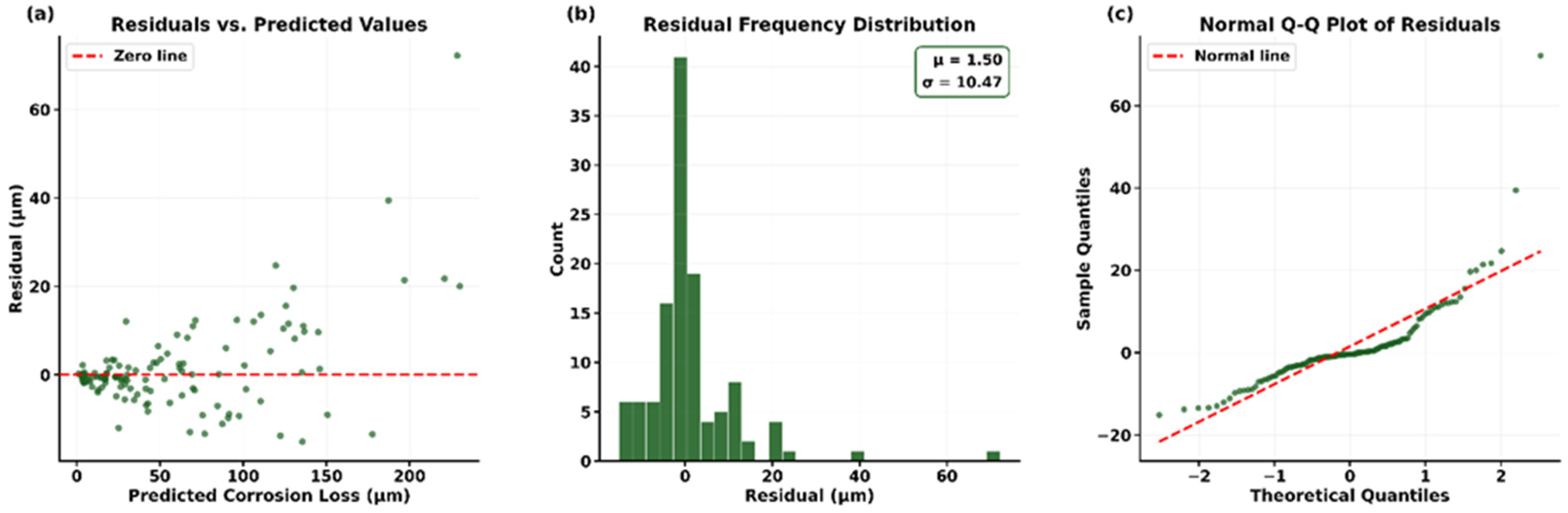
Model performance was quantified using four metrics evaluated on the held-out test set on the original (µm) scale: coefficient of determination (R2), root mean squared error (RMSE, µm), mean absolute error (MAE, µm), and mean absolute percentage error (MAPE, %). Five-fold cross-validation R2 (CV-R2) on the training set was used as the primary model selection criterion. The best model was further evaluated using residual diagnostics: residuals vs. predicted, residual frequency histogram, and normal quantile-quantile (Q-Q) plots.

2.5. SHAP Interpretability Analysis

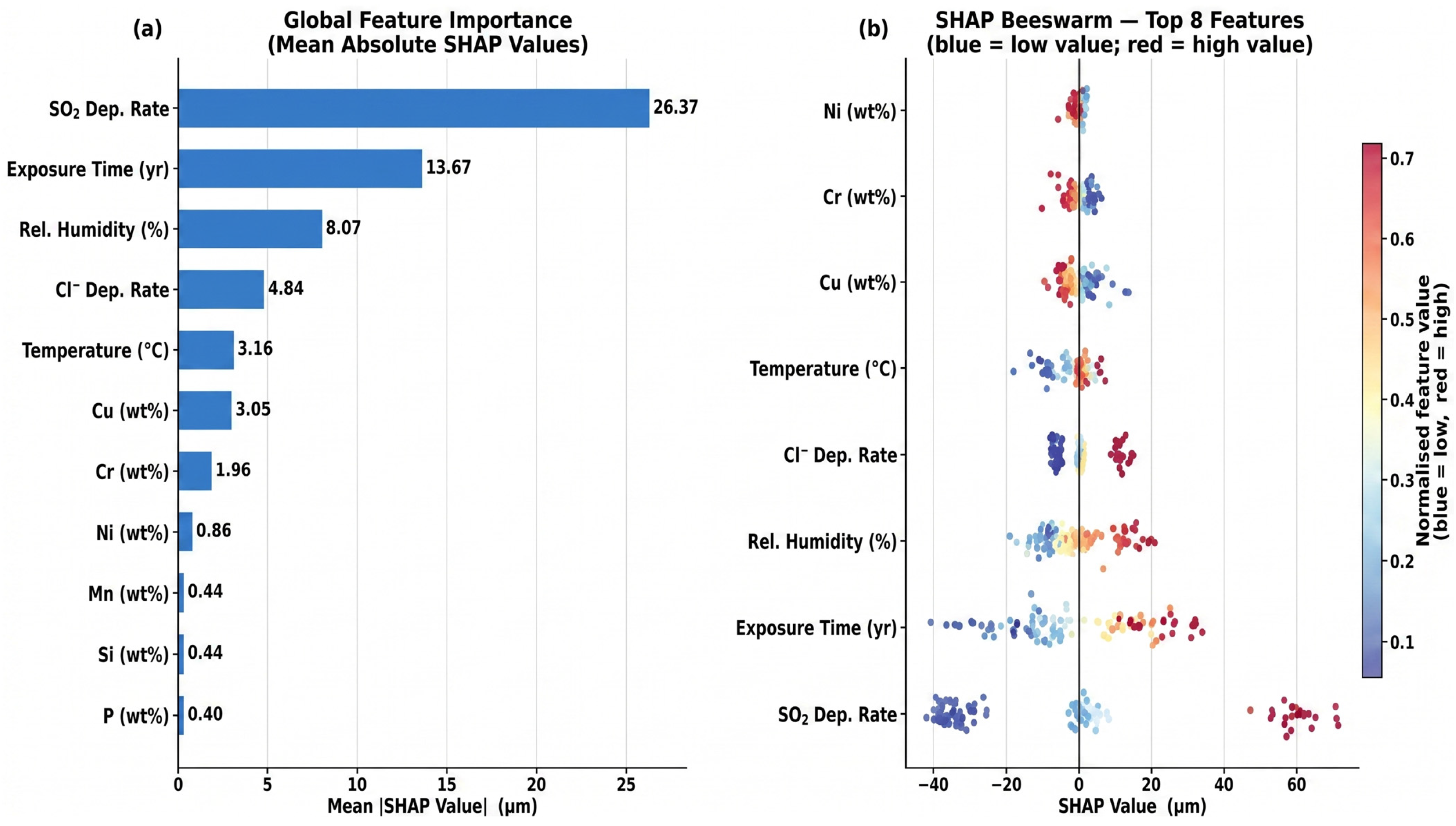
Global feature importance and directional feature effects were quantified using SHAP (SHapley Additive exPlanations) analysis applied to the XGBoost model via the exact TreeExplainer algorithm (SHAP v0.44) [35]. XGBoost was selected for SHAP analysis because its implementation enables exact Shapley value computation for tree ensembles; the near-identical CV-R2 of GBR (0.969) and XGBoost (0.960) indicates both models learned equivalent feature relationships, supporting the transferability of the SHAP-derived importance rankings. The tree explainer computes the exact Shapley values for tree ensembles without a Monte Carlo approximation. Global importance was ranked by the mean |SHAP value| across all test samples. A beeswarm plot simultaneously displayed the magnitude and direction of feature effects for the eight most influential features, with color encoding indicating the feature value magnitude (blue = low, red = high).

3. Results

3.1. Dataset Characteristics and Correlation Analysis

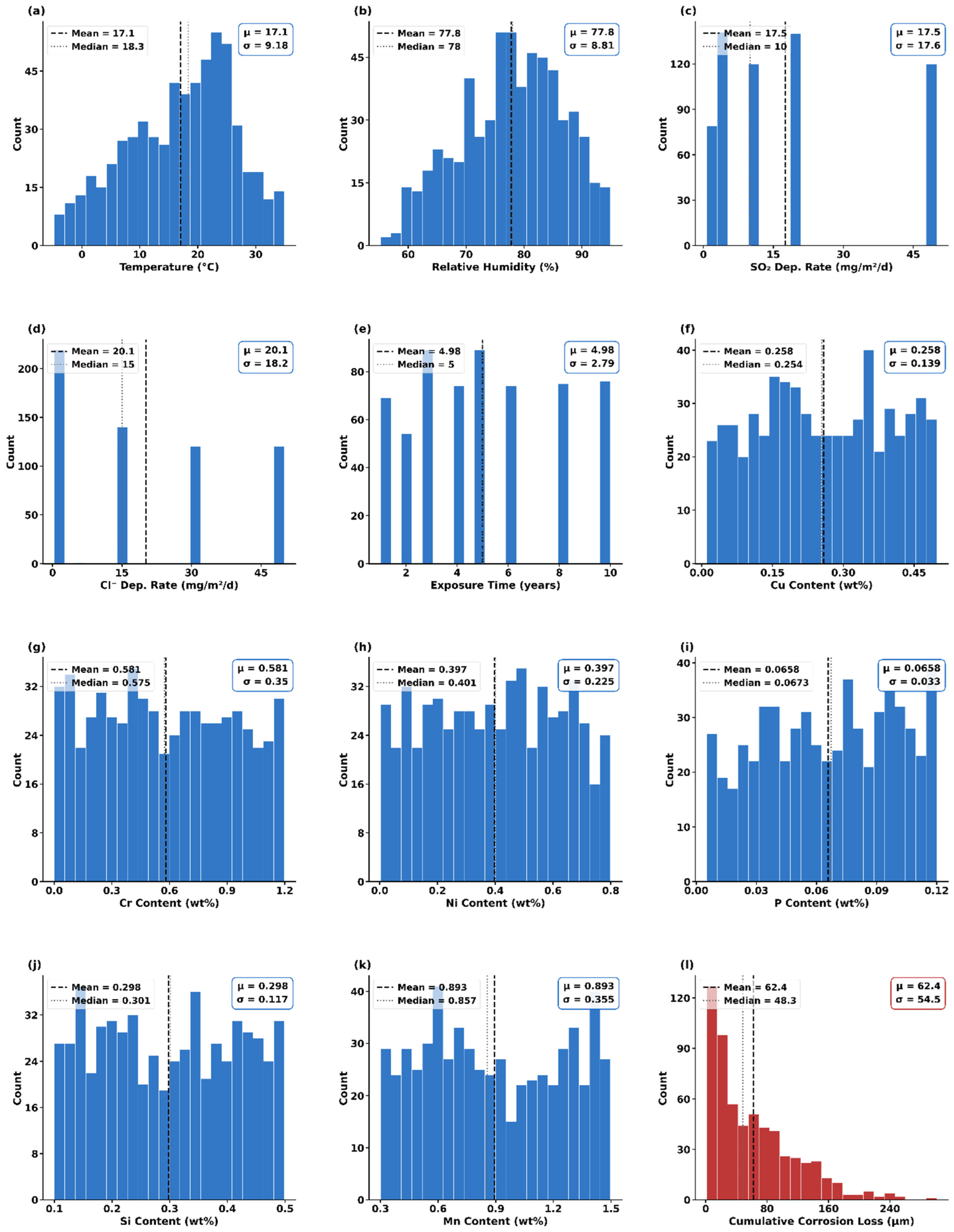
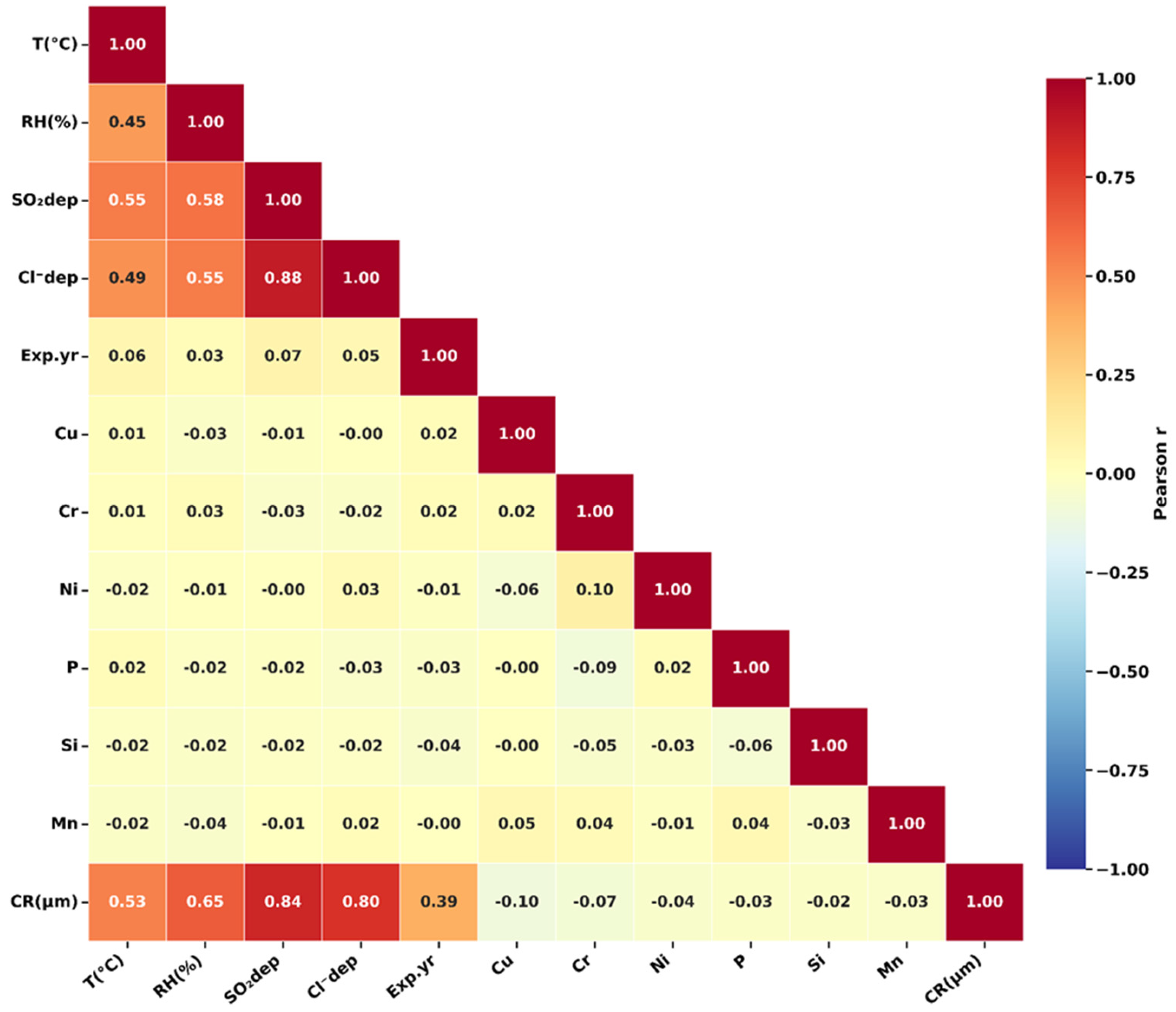
The constructed dataset of 600 samples spans cumulative corrosion losses from 1.3 to 300.8 µm (mean = 62.4 µm, SD = 54.5 µm, median = 48.3 µm). The ISO 9223 category distribution C2 (33%, n = 200), C3 (18%, n = 105), C4 (18%, n = 107), C5 (29%, n = 172), and CX (3%, n = 16) reflects the stratified construction targeting a broad corrosivity range, consistent with the ISOCORRAG global exposure database [23]. Feature distributions and the target variable are shown in Figure 1. Pearson’s correlation analysis with cumulative corrosion loss (Figure 2) yielded the following verified values: SO2 deposition rate (r = 0.843), Cl deposition rate (r = 0.796), relative humidity (r = 0.649), temperature (r = 0.533), and exposure time (r = 0.392). Among the material composition features, Cu showed the strongest negative correlation (r = −0.096), followed by Cr (r = −0.071), Ni (r = −0.040), Mn (r = −0.033), P (r = −0.030), and Si (r = −0.025). The dominance of SO2 and Cl deposition in the linear correlations (r > 0.79) reflects their explicit appearance as power-law terms in the ISO 9223 DRF. The moderate correlations of RH and T (r = 0.649 and 0.533, respectively) reflect their role as exponential modifiers. The weak linear correlations of material features (|r| < 0.10) confirm that composition effects are largely nonlinear and multiplicative, precisely the type of relationship that tree-based ML models are designed to capture [29,30].

3.2. Comparative Model Performance

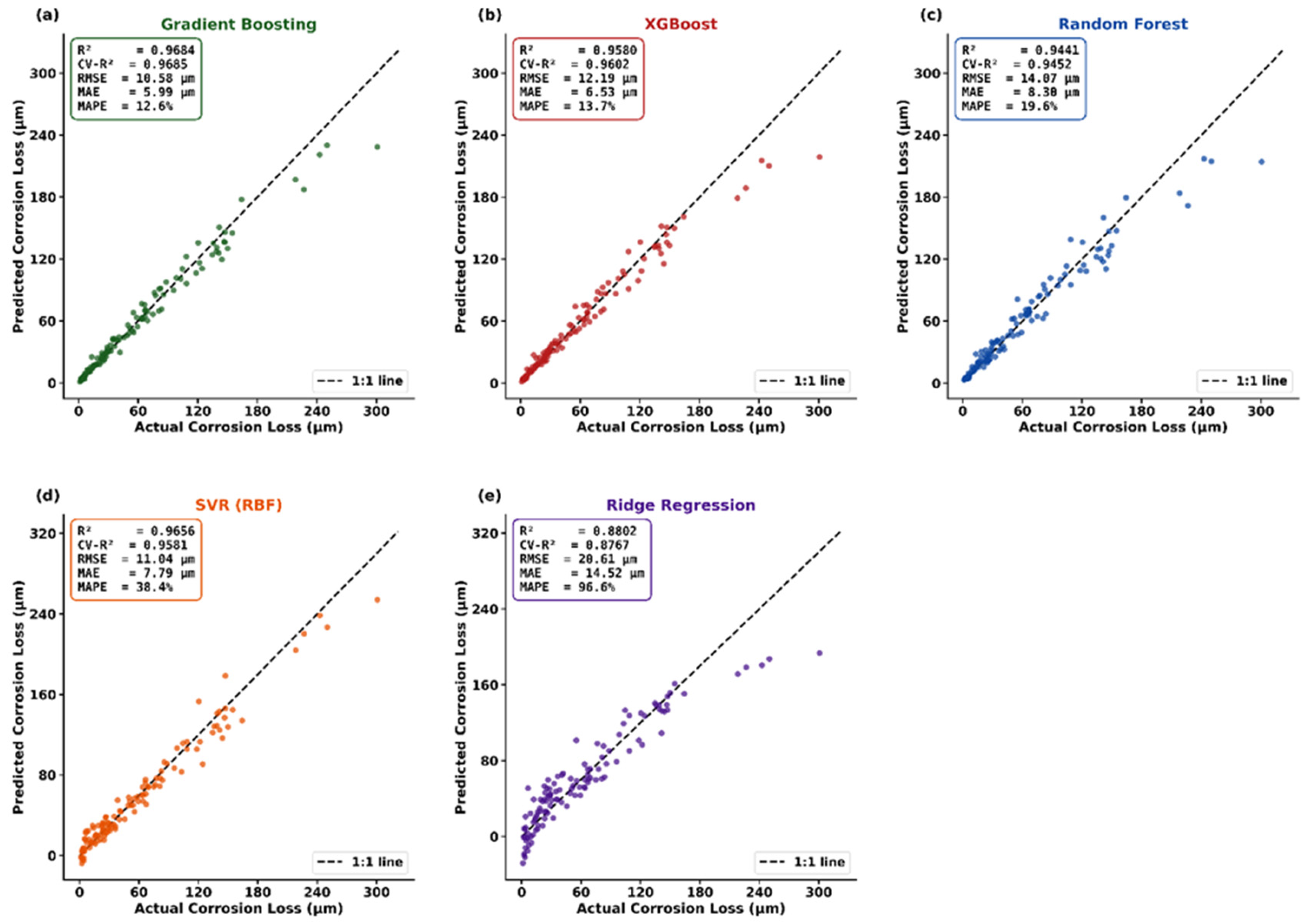
Table 2 presents the complete performance metrics for all five ML models on the held-out test set and five-fold cross-validation. Gradient boosting achieved the highest overall performance, with test set R2 = 0.968, CV-R2 = 0.969, RMSE = 10.58 µm, MAE = 5.99 µm, and MAPE = 12.6%. XGBoost was the close second, with R2 = 0.958 and CV-R2 = 0.960. SVR achieved test set R2 = 0.966; however, it recorded the highest MAPE (38.4%) among all models, reflecting the known structural difficulty of margin-based kernel methods with highly skewed, heavy-tailed target distributions. The high-CCL CX-category samples deviate substantially from the central distribution, which the ε-insensitive loss function of SVR cannot adequately accommodate, regardless of kernel choice. The SVR hyperparameters (C = 500, ε = 1.5, RBF kernel) were selected based on published recommendations for corrosion datasets [13,14,15] and validated by 5-fold cross-validation, representing a well-tuned configuration for this class of problem. RF achieved R2 = 0.944 and CV-R2 = 0.945. Ridge regression underperformed (R2 = 0.880, MAPE = 96.6%), confirming that the nonlinear, multiplicative structure of the ISO 9223 DRF cannot be captured by linear models. The GBR result (CV-R2 = 0.969) is consistent with Kuang and Long [15], who identified Cl and SO2 as primary environmental predictors by using ensemble ML methods, and Dong et al. [18], who reported R2 = 0.918 for RF in steel soil corrosion. The superior ensemble performance relative to linear and kernel methods is consistent with the review by Coelho et al. [13] and the findings of Yan et al. [14] for marine atmospheric corrosion datasets. Figure 3a–e shows the predicted vs. actual corrosion loss scatter plots for all five models, and Figure 4a–c compares te R2 scores, RMSE/MAE, and MAPE, respectively.

3.3. Residual Diagnostics

Before discussing residual diagnostics, it is important to contextualize the model prediction errors against the inherent uncertainty of real atmospheric corrosion measurements. Gravimetric corrosion loss measurements in standardized atmospheric exposure studies typically carry uncertainties of 5%–15%, arising from incomplete corrosion product removal, specimen surface heterogeneity, weighing instrument precision, and environmental fluctuations during exposure [27]. The GBR model achieves a MAE = 5.99 µm and MAPE = 12.6% on the test set. When normalized to the mean corrosion loss of 62.4 µm, the MAE corresponds to approximately 9.6%, which falls well within the 5%–15% range of typical experimental gravimetric uncertainty. This confirms that the model prediction error is not significantly larger than what would be observed between replicate experimental measurements under identical conditions. It is acknowledged that the synthetic nature of the training dataset means that additional, unmodeled environmental variability present in real-world scenarios, including time-varying pollution levels, surface contamination history, and microclimate effects, may result in larger deviations when applied to independently measured field data. Validation against experimental datasets from ISOCORRAG and MICAT is recommended as a critical next step.
Figure 5 presents residual diagnostics for the best-performing gradient boosting model. Figure 5a (residuals vs. predicted) shows a random scatter centered at zero across the full prediction range, with no systematic bias, heteroscedasticity, or trend, confirming that the model captures the main variance structure of the data. Figure 5b (residual frequency histogram) closely approximates a normal distribution centered near zero (μ = 1.50 µm, σ = 10.47 µm). Figure 5c (normal Q-Q plot) shows good alignment with the theoretical quantile line across the central range, with a mild deviation at the tails corresponding to the high-CCL CX-category samples, which is physically expected given the inherently higher variability in extreme marine-industrial environments [23]. Overall, the residual diagnostics confirm that the GBR satisfies the key assumptions of a well-fitting regression model.

3.4. SHAP Feature Importance and Interpretability

Although SHAP analysis was applied to XGBoost rather than the optimal GBR model, the near-identical cross-validation performance of both models (CV-R2: GBR = 0.969, XGBoost = 0.960) confirms they captured equivalent dominant patterns in the data, supporting the consistency of the reported feature importance hierarchy across both gradient boosting frameworks. The SHAP analysis of the XGBoost model (Figure 6) provides a fully interpretable and physically consistent feature importance ranking. The global importance order (mean |SHAP|), shown in Figure 6a, is as follows: SO2 deposition rate (Pd, mean |SHAP| = 26.37 µm) > exposure time (13.67 µm) > relative humidity (RH, 8.07 µm) > Cl deposition rate (Sd, 4.84 µm) > temperature (T, 3.16 µm) > Cu content (3.05 µm) > Cr content (1.96 µm) > Ni content (0.86 µm). The top ranking of the SO2 deposition rate reflects its appearance as a dominant power-law term (Pd^0.52) in the ISO 9223 DRF [10]. The second-highest importance of exposure time above Cl and T reflects the ISO 9224 power-law kinetics; because C(t) = C1·t0.5, the progressive accumulation of corrosion loss over the 1–10-year range creates a large, systematic SHAP contribution that exceeds that of individual environmental variables. The high third-place ranking of RH reflects its exponential role in both DRF terms across the broad 55%–95% range sampled. Material features (Cu, Cr, and Ni) rank below all environmental predictors, consistent with their entry only through the multiplicative material factor [10]. The beeswarm plot (Figure 6b) confirms that high Pd, high Sd, high RH, and high T consistently increase predicted corrosion (positive SHAP values), whereas high Cu and Cr contents consistently decrease predicted corrosion loss (negative SHAP values). These directional effects are exactly predicted by the underlying physical chemistry: high Cu promotes the formation of a dense, protective goethite inner rust layer [25], whereas high Cr contributes to a passive Cr-enriched oxide formation that retards iron dissolution [26].
The environmental predictors, identified by SHAP, are consistent with independent experimental literature: SO2 and Cl deposition, as primary drivers, align with Kuang and Long [15], while the importance of RH and T is consistent with Li et al. [17] (Cl, TOW, and T dominant via ACM sensor data at six Chinese sites) and Yan et al. [14] (Cl and RH as key predictors in Japanese marine atmosphere). The high second-place ranking of exposure time in this study above Cl and T is a direct consequence of the multi-year prediction scope (1–10 years) and the ISO 9224 power-law kinetics embedded in the dataset. It distinguishes this study from single-year corrosion rate studies, in which exposure time is not an input feature. The convergence of environmental SHAP rankings with independent experimental studies and with the explicit physics of ISO 9223 and ISO 9224 provides strong validation of the physical consistency of the learned model. It confirms that the model captures the underlying corrosion physics rather than performing purely statistical fitting.

3.5. Corrosion Loss by ISO 9223 Category and Alloying Element Effects

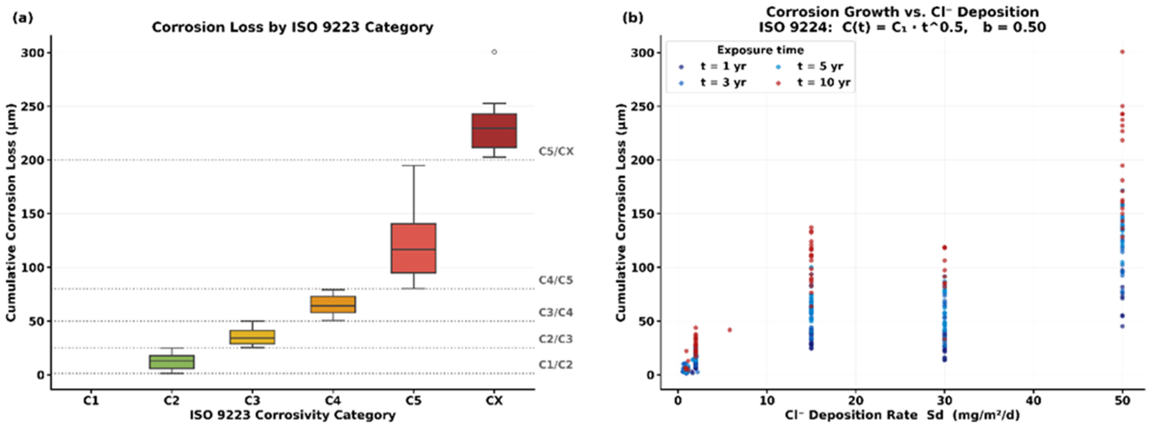
Figure 7 presents the distribution of the cumulative corrosion loss across ISO 9223 corrosivity categories and its dependence on the Cl deposition rate at different exposure times. Figure 7a (the box-and-whisker plot of cumulative corrosion loss distribution by ISO 9223 corrosivity category) confirms the expected severity hierarchy (CX > C5 > C4 > C3 > C2), with verified median CCL values of 229.3, 116.6, 64.3, 34.1, and 12.8 µm for CX, C5, C4, C3, and C2, respectively, which are consistent with the 2012 thresholds [10] and validate the physical consistency of the synthetic dataset. Figure 7b (scatter plot) demonstrates the power-law growth of corrosion with exposure time: for a given Cl deposition level, the cumulative corrosion loss at t = 10 years is approximately √10 ≈ 3.16× higher than that at t = 1 year, which is consistent with the ISO 9224 b = 0.50 exponent [11,24].
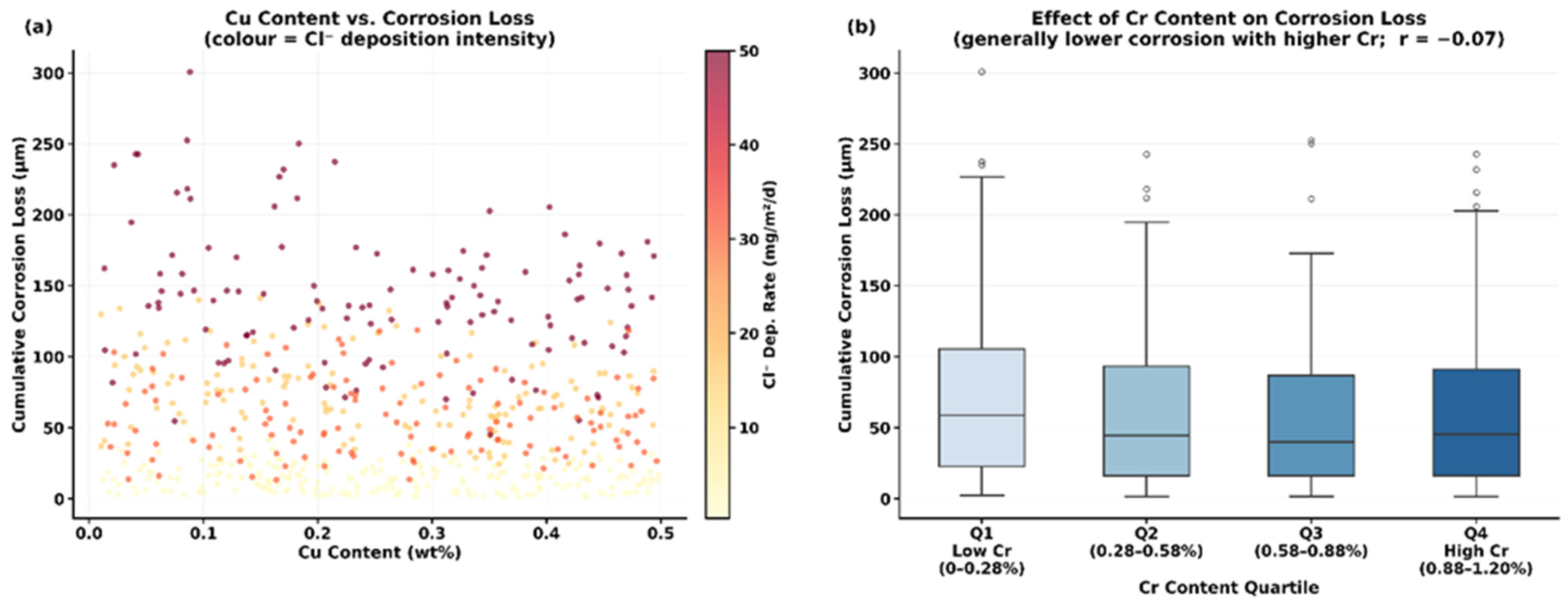
Figure 8 shows the effects of key alloying elements on the cumulative corrosion loss. Figure 8a is a scatter plot of the Cu content versus corrosion loss, colored by the Cl deposition intensity, revealing an overall negative trend (Pearson r = −0.096). This is most visible at high Cl deposition levels, which is consistent with the beneficial role of Cu documented in the weathering steel review by Morcillo et al. [25], where Cu content was identified as a key factor in reducing atmospheric corrosion loss through goethite inner rust layer formation. Figure 8b (quartile boxplot of Cr content) shows a general decrease in the median corrosion loss from Q1 (0–0.28 wt%, median CCL = 58.8 µm) to Q3 (0.58–0.88 wt%, median CCL = 39.9 µm), with Q4 (0.88–1.20 wt%) showing a slight uptick to 45.4 µm. This non-monotonic Q3–Q4 pattern is physically consistent with the weak Pearson correlation (r = −0.07) between Cr and CCL, reflecting the dominant role of environmental factors in this dataset. The overall lower median CCL in Q2–Q4 relative to Q1 is qualitatively consistent with the corrosion-inhibiting role of Cr documented by Díaz et al. [26].

4. Discussion

Table 3 presents a systematic comparison of the present study with the most relevant published ML-based corrosion prediction studies. Yan et al. [14] applied six ML algorithms (RF, GBDT, XGBoost, SVR, MLR, and RR) to predict the annual corrosion rate of low-alloy steels at three Japanese marine atmospheric exposure sites by using the NIMS CoDS experimental database (n = 306), with exposure time included as an explicit input and with SHAP analysis applied to evaluate feature contributions. RF achieved R2 = 0.94 (training) and R2 = 0.73 (test set), and SHAP analysis identified alloying element content, chloride deposition rate, and precipitation as dominant features in early exposure years—directionally consistent with the findings of the present study. Zhi et al. [16] developed an SVR model for atmospheric corrosion of Q235 carbon steel at ten Chinese sites by using a hybrid RF + Spearman coefficient approach to screen 12 environmental factors to six to seven key inputs; separate SVR models were trained per exposure year without exposure time used as an explicit input feature, and prediction accuracy was reported as MAPE rather than R2. Narayana et al. [21] applied a backpropagation ANN (6-11-11-1 architecture, n = 130) to predict single-year carbon steel corrosion rates from six atmospheric inputs, achieving R2 = 0.776 on the test set without exposure time being used as a model input, or SHAP analysis. Dong et al. [18] achieved RF R2 = 0.987 on a soil corrosion dataset (n = 1428), with exposure time used as an explicit feature; SHAP analysis was not performed, and the soil corrosion mechanism and dataset scale differ substantially from atmospheric corrosion. Kuang and Long [15] benchmarked six ML algorithms, including XGBoost, for the atmospheric corrosion rate prediction of low-alloy steels with exposure time and SHAP analysis via a property transformation approach, making their study methodologically the most similar to the present work. The present study advances beyond all these benchmarks by (1) predicting multi-year cumulative corrosion loss (CCL, µm) over 1–10 years within a single trained model rather than single-year rates; (2) constructing a physics-grounded dataset of 600 samples from ISO 9223:2012 and ISO 9224:2012, ensuring full physical self-consistency across C2–CX corrosivity categories; (3) achieving GBR test set R2 = 0.968 and CV-R2 = 0.969; and (4) providing SHAP analysis that quantitatively confirms consistency with both the ISO 9223 dose–response function and ISO 9224 power-law kinetics—a combination of multi-year scope, physics-grounded construction, and SHAP-validated physical consistency, which are not present in any single prior study to the best of our knowledge.
The principal finding of this study is that gradient boosting achieves CV-R2 = 0.969 and test set R2 = 0.968 for the multi-year cumulative atmospheric corrosion loss prediction of low-alloy steels on the original (untransformed) corrosion scale, establishing a new ML benchmark for this specific prediction task. This performance level is consistent with Kuang and Long [15] and Dong et al. [18] and represents a significant improvement over earlier studies that achieved lower test set R2 values by omitting exposure time as a feature [14]. The inclusion of exposure time as an explicit feature, guided by ISO 9224 power-law kinetics, was critical: it enables the model to capture the well-documented progressive accumulation of corrosion loss over multi-year service and makes the model directly applicable to service-life planning over the 1–10-year horizon, which is most relevant to coating maintenance scheduling.
The superiority of GBR and XGBoost over SVR and ridge regression has a clear physical interpretation. The ISO 9223 DRF is inherently multiplicative and nonlinear, is a sum of two power-law terms in Pd and Sd, each multiplied by an exponential function of RH and T, and is a mathematical structure that gradient boosting trees can approximate through recursive splits, which is beyond the capabilities of linear and even kernel models [29,30,32]. The SHAP-validated importance hierarchy (SO2 dep. > Exposure time > RH > Cl dep. > T > Cu > Cr > Ni) is consistent with the explicit structure of both ISO 9223 and ISO 9224: SO2 deposition appears in a power-law exponent (Pd0.52), giving it disproportionate leverage, while exposure time governs multi-year accumulation via C(t) = C1·t0.5, producing large systematic SHAP contributions across the 1–10-year range. The ranking of RH (third) above Cl (fourth) reflects its exponential role in both DRF terms across the broad 55%–95% range sampled. This observation confirms that ML does not merely interpolate data but correctly recovers the dominant physics encoded in both the ISO 9223 dose–response function and the ISO 9224 kinetic model.
The SHAP-validated feature importance hierarchy provides direct mechanistic insight into atmospheric corrosion physics. The dominance of the SO2 deposition rate (mean |SHAP| = 26.37 µm) is consistent with its well-established electrochemical role: SO2 reacts with the rust layer to form hygroscopic iron sulfates (FeSO4·nH2O), which prevent the formation of a stable, protective α-FeOOH (goethite) patina and sustain the electrochemical corrosion cycle by maintaining electrolyte contact at the steel surface [12,15]. The second-place ranking of exposure time (13.67 µm) reflects the ISO 9224 power-law kinetics C(t) = C1·t0.5: initial rapid oxide formation transitions to diffusion-controlled growth as the rust layer thickens, and the ML model correctly learns this nonlinear time-dependence. The third-place ranking of relative humidity (8.07 µm) reflects its exponential role in both ISO 9223 DRF terms, governing the time of wetness and therefore the duration of electrochemical activity at the steel surface. Among material features, Cu (mean |SHAP| = 3.05 µm, negative) promotes the formation of a denser, more adherent inner rust layer dominated by goethite (α-FeOOH), which acts as a diffusion barrier that reduces ionic transport to the steel substrate [25]. Cr (1.96 µm, negative) substitutes into the rust structure and promotes passive Cr-enriched inner oxide formation, retarding iron dissolution [26]. The weak linear Pearson correlations of material features (|r| < 0.10, Figure 2), despite their non-negligible SHAP contributions, confirm that composition effects operate nonlinearly through multiplicative interactions with environmental variables, which is exactly the type of relationship that tree-based ensemble models are designed to capture [29,30].
These results have direct implications for the selection of protective coatings and alloy designs. The SHAP analysis shows that in C5 and CX environments (high Cl and SO2), the environmental factors are so dominant that alloying element effects become secondary, underscoring that barrier coatings (epoxy, polyurethane, zinc-rich primers) providing physical isolation from the aggressive atmosphere are the primary mitigation strategy in such environments [3,4,5,8]. Advanced surface engineering approaches, such as superhydrophobic coatings with intermetallic phase in situ pinning, have further demonstrated enhanced corrosion protection through surface microstructure control [36]. In contrast, in C2–C3 environments, the material features (Cu, Cr) showed larger relative SHAP contributions, suggesting that alloying-based solutions (weathering steels, Corten grades) can be effective alternatives to organic coatings, which is consistent with the recommendations of Morcillo et al. [25] and the coating selection guidance of ISO 12944. The ML framework developed here provides a quantitative basis for environment-specific material selection decisions.
The present approach directly extends the work of Tiwari et al. [20] on ML-based atmospheric corrosion prediction by introducing exposure time as an explicit feature, predicting multi-year cumulative loss rather than single-year rates, and providing full SHAP interpretability, which is not present in that study. It also extends the ANN-based carbon steel corrosion modeling of Narayana et al. [21] by comparing five ML algorithm families under rigorous cross-validation and providing SHAP-validated feature importance rankings. The corrosion-specific ensemble framework presented herein complements the ML-based mechanical property prediction of Xiong et al. [22], demonstrating that tree-based ensembles are equally effective for both the mechanical and degradation property predictions of low-alloy steels. The physics-grounded dataset construction strategy, based on ISO 9223/9224 equations with stratified environmental sampling, addresses a recognized limitation in corrosion ML datasets, noted by Coelho et al. [13], regarding the need for physically consistent training data.
The limitations of this study should be acknowledged for future advanced studies. The dataset was constructed from a physics-grounded synthetic framework (ISO 9223:2012 DRF + ISO 9224:2012 kinetics) with ±5% Gaussian noise rather than direct experimental measurements. While this approach ensures physical consistency, full control over the feature space, and sufficient sample size (n = 600) for reliable ML training factors that are difficult to achieve simultaneously with scarce, heterogeneous field datasets, it cannot capture all sources of variability present in real atmospheric exposure data, including time-varying pollution levels, wet/dry cycling, surface contamination history, and microclimate effects. The ±5% Gaussian noise model further assumes independent, identically distributed errors, whereas real measurement errors in gravimetric corrosion studies arise from multiple sources (incomplete rust removal, specimen surface heterogeneity, weighing precision, environmental fluctuations) and may follow non-Gaussian, heteroscedastic distributions that vary with environmental aggressiveness. Additionally, the power-law exponent b = 0.50, adopted per ISO 9224 as a standardized reference value, is an approximation: in practice, b varies with steel composition (typically 0.3–0.7), environmental aggressivity, and exposure duration, generally decreasing as a more protective rust layer develops [24]. Future work should validate the framework against large experimental datasets from ISOCORRAG/MICAT, incorporate additional features (time of wetness, wind speed, annual precipitation, and protective rust layer maturity indices), and explore transfer learning strategies to adapt the present model to real-world field conditions.

5. Conclusions

This study benchmarked five machine learning algorithms for predicting the multi-year cumulative atmospheric corrosion loss of low-alloy steels by using a 600-sample dataset that was grounded in the exact ISO 9223:2012 dose–response function and ISO 9224:2012 power-law kinetics. The key verified findings are as follows:
(1) Gradient boosting achieved the best overall performance, with a test set R2 of 0.968, CV-R2 of 0.969, RMSE of 10.58 µm, MAE of 5.99 µm, and MAPE of 12.6% on the original-scale cumulative corrosion loss. XGBoost was a close second (R2 = 0.958, CV-R2 = 0.960). Both ensemble methods significantly outperformed SVR, RF, and ridge regression, confirming that the nonlinear physics of atmospheric corrosion requires ensemble tree-based models for accurate prediction.
(2) The inclusion of exposure time as an explicit feature, guided by ISO 9224 power-law kinetics, was critical for achieving an R2 > 0.90 in cumulative loss prediction and for making the model applicable to multi-year service-life planning.
(3) The SHAP analysis identified the SO2 deposition rate and exposure time as the two most influential predictors, followed by relative humidity, Cl deposition rate, and temperature, which is consistent with the ISO 9223:2012 DRF structure and ISO 9224:2012 power-law kinetics.
(4) ISO 9223 category-wise analysis confirmed the expected corrosion severity hierarchy (CX > C5 > C4 > C3 > C2) and validated the ISO 9224 power-law growth trajectory, providing physical sanity checks for the model.
(5) The interpretable physics-consistent ML framework established herein provides a quantitative tool for corrosion-resistant alloy screening, protective coating selection across C2–CX environments, and multi-year service-life planning for low-alloy steel infrastructure. Future work should incorporate a variable power-law exponent b that is informed by steel composition, environmental aggressivity, and exposure duration rather than the fixed ISO 9224 reference value of b = 0.50 so as to improve the physical realism of the kinetic model and extend the framework to a broader range of steel grades and real-world exposure conditions.
Future work should extend SHAP interpretability analysis to the GBR model directly and incorporate pairwise SHAP interaction values, particularly for the SO2 × exposure time and Cu × SO2 feature pairs, to provide deeper mechanistic insight into the nonlinear multi-factor interactions governing long-term atmospheric corrosion.

Supplementary Materials

The following supporting information can be downloaded at: https://www.mdpi.com/article/10.3390/coatings16040488/s1, Table S1: Supplementary_Data Table S1.

Author Contributions

Conceptualization, S.T. and N.P.; methodology, S.T. and S.J.H.; software, S.T.; validation, S.J.H. and S.T.; formal analysis and investigation, S.T. and S.J.H.; resources, N.P. and S.T.; data curation, S.J.H. and S.T.; writing—original draft preparation, S.T.; writing—review and editing, S.T. and N.P.; visualization, S.J.H. and S.T.; supervision, N.P. and S.T.; project administration, and funding acquisition, N.P. All authors have read and agreed to the published version of the manuscript.

Funding

This research was supported by the Regional Innovation System & Education (RISE) program through the Gyeongbuk RISE CENTER, funded by the Ministry of Education (MOE) and the Gyeongsangbuk-do, Republic of Korea (2025-RISE-15-115).

Institutional Review Board Statement

Not applicable.

Informed Consent Statement

Not applicable.

Data Availability Statement

The data supporting the findings of this study are available in the Supplementary File. Additional details are available from the corresponding author upon reasonable request.

Conflicts of Interest

The authors declare no conflicts of interest.

References

  1. Hou, B.; Li, X.; Ma, X.; Du, C.; Zhang, D.; Zheng, M.; Xu, W.; Lu, D.; Ma, F. The Cost of Corrosion in China. npj Mater. Degrad. 2017, 1, 4. [Google Scholar] [CrossRef] [Scilit]
  2. Koch, G.; Varney, J.; Thompson, N.; Moghissi, O.; Gould, M.; Payer, J. International Measures of Prevention, Application, and Economics of Corrosion Technologies Study (IMPACT); NACE International: Houston, TX, USA, 2016. [Google Scholar]
  3. Sørensen, P.A.; Kiil, S.; Dam-Johansen, K.; Weinell, C.E. Anticorrosive Coatings: A Review. J. Coat. Technol. Res. 2009, 6, 135–176. [Google Scholar] [CrossRef] [Scilit]
  4. Dalmora, G.P.V.; Borges Filho, E.P.; Maraschin Conterato, A.A.; Roso, W.S.; Pereira, C.E.; Dettmer, A. Methods of Corrosion Prevention for Steel in Marine Environments: A Review. Results Surf. Interfaces 2025, 18, 100430. [Google Scholar] [CrossRef] [Scilit]
  5. Lazorenko, G.; Kasprzhitskii, A.; Nazdracheva, T. Anti-Corrosion Coatings for Protection of Steel Railway Structures Exposed to Atmospheric Environments: A Review. Constr. Build. Mater. 2021, 288, 123115. [Google Scholar] [CrossRef] [Scilit]
  6. Melchers, R.E. Predicting Long-Term Corrosion of Metal Alloys in Physical Infrastructure. npj Mater. Degrad. 2019, 3, 4. [Google Scholar] [CrossRef] [Scilit]
  7. Chen, W.; Ma, L.; Li, Y.; Wu, D.; Zhou, K.; Wang, J.; Chen, Z.; Guo, X.; Li, Z.; Chowwanonthapunya, T.; et al. Prediction of Coating Degradation Based on “Environmental Factors–Physical Property–Corrosion Failure” Two-Stage Machine Learning. npj Mater. Degrad. 2025, 9, 67. [Google Scholar] [CrossRef] [Scilit]
  8. Liu, C.; Bi, Q.; Leyland, A.; Matthews, A. An Electrochemical Impedance Spectroscopy Study of the Corrosion Behaviour of PVD Coated Steels in 0.5 N NaCl Aqueous Solution: Part II: EIS Interpretation of Corrosion Behaviour. Corros. Sci. 2003, 45, 1257–1273. [Google Scholar] [CrossRef] [Scilit]
  9. López-Ortega, A.; Bayón, R.; Arana, J.L. Evaluation of Protective Coatings for High-Corrosivity Category Atmospheres in Offshore Applications. Materials 2019, 12, 1325. [Google Scholar] [CrossRef] [Scilit]
  10. ISO 9223:2012; Corrosion of Metals and Alloys—Corrosivity of Atmospheres—Classification, Determination and Estimation. ISO: Geneva, Switzerland, 2012.
  11. ISO 9224:2012; Corrosion of Metals and Alloys—Corrosivity of Atmospheres—Guiding Values for the Corrosivity Categories. ISO: Geneva, Switzerland, 2012.
  12. Tidblad, J.; Kreislová, K.; Faller, M.; la Fuente, D.; Yates, T.; Verney-Carron, A.; Grøntoft, T.; Gordon, A.; Hans, U. ICP Materials Trends in Corrosion, Soiling and Air Pollution (1987–2014). Materials 2017, 10, 969. [Google Scholar] [CrossRef] [Scilit]
  13. Coelho, L.B.; Zhang, D.; Van Ingelgem, Y.; Steckelmacher, D.; Nowé, A.; Terryn, H. Reviewing Machine Learning of Corrosion Prediction in a Data-Oriented Perspective. npj Mater. Degrad. 2022, 6, 8. [Google Scholar] [CrossRef] [Scilit]
  14. Yan, L.; Diao, Y.; Lang, Z.; Gao, K. Corrosion Rate Prediction and Influencing Factors Evaluation of Low-Alloy Steels in Marine Atmosphere Using Machine Learning Approach. Sci. Technol. Adv. Mater. 2020, 21, 359–370. [Google Scholar] [CrossRef] [Scilit]
  15. Kuang, J.; Long, Z. Prediction Model for Corrosion Rate of Low-Alloy Steels under Atmospheric Conditions Using Machine Learning Algorithms. Int. J. Miner. Metall. Mater. 2024, 31, 337–350. [Google Scholar] [CrossRef] [Scilit]
  16. Zhi, Y.; Jin, Z.; Lu, L.; Yang, T.; Zhou, D.; Pei, Z.; Wu, D.; Fu, D.; Zhang, D.; Li, X. Improving Atmospheric Corrosion Prediction through Key Environmental Factor Identification by Random Forest-Based Model. Corros. Sci. 2021, 178, 109084. [Google Scholar] [CrossRef] [Scilit]
  17. Li, Q.; Xia, X.; Pei, Z.; Cheng, X.; Zhang, D.; Xiao, K.; Wu, J.; Li, X. Long-Term Corrosion Monitoring of Carbon Steels and Environmental Correlation Analysis via the Random Forest Method. npj Mater. Degrad. 2022, 6, 1. [Google Scholar] [CrossRef] [Scilit]
  18. Dong, Z.; Ding, L.; Meng, Z.; Xu, K.; Mao, Y.; Chen, X.; Ye, H.; Poursaee, A. Machine Learning-Based Corrosion Rate Prediction of Steel Embedded in Soil. Sci. Rep. 2024, 14, 18194. [Google Scholar] [CrossRef] [Scilit]
  19. Liu, Y.; Chen, K.; Kumar, A.; Patnaik, P. Principles of Machine Learning and Its Application to Thermal Barrier Coatings. Coatings 2023, 13, 1140. [Google Scholar] [CrossRef] [Scilit]
  20. Tiwari, S.; Dash, K.; Park, N.; Reddy, N.G.S. Machine Learning-Based Prediction of Atmospheric Corrosion Rates Using Environmental and Material Parameters. Coatings 2025, 15, 888. [Google Scholar] [CrossRef] [Scilit]
  21. Narayana, P.L.; Tiwari, S.; Maurya, A.K.; Ishtiaq, M.; Park, N.; Reddy, N.G.S. Quantitative and Qualitative Analysis of Atmospheric Effects on Carbon Steel Corrosion Using an ANN Model. Metals 2025, 15, 607. [Google Scholar] [CrossRef] [Scilit]
  22. Xiong, J.; Zhang, T.; Shi, S. Machine Learning of Mechanical Properties of Steels. Sci. China Technol. Sci. 2020, 63, 1247–1255. [Google Scholar] [CrossRef] [Scilit]
  23. Chico, B.; la Fuente, D.; Díaz, I.; Simancas, J.; Morcillo, M. Annual Atmospheric Corrosion of Carbon Steel Worldwide. An Integration of ISOCORRAG, ICP/UNECE and MICAT Databases. Materials 2017, 10, 601. [Google Scholar] [CrossRef] [Scilit]
  24. Panchenko, Y.M.; Marshakov, A.I. Long-Term Prediction of Metal Corrosion Losses in Atmosphere Using a Power-Linear Function. Corros. Sci. 2016, 109, 217–229. [Google Scholar] [CrossRef] [Scilit]
  25. Morcillo, M.; Chico, B.; Díaz, I.; Cano, H.; de la Fuente, D. Atmospheric Corrosion Data of Weathering Steels. A Review. Corros. Sci. 2013, 77, 6–24. [Google Scholar] [CrossRef] [Scilit]
  26. Díaz, I.; Cano, H.; Lopesino, P.; de la Fuente, D.; Chico, B.; Jiménez, J.A.; Medina, S.F.; Morcillo, M. Five-Year Atmospheric Corrosion of Cu, Cr and Ni Weathering Steels in a Wide Range of Environments. Corros. Sci. 2018, 141, 146–157. [Google Scholar] [CrossRef] [Scilit]
  27. ISO 8407:2021; Corrosion of Metals and Alloys—Removal of Corrosion Products from Corrosion Test Specimens. ISO: Geneva, Switzerland, 2021.
  28. Strieška, M.; Koteš, P. Sensitivity of Dose-Response Function for Carbon Steel under Various Conditions in Slovakia. Transp. Res. Procedia 2019, 40, 912–919. [Google Scholar] [CrossRef] [Scilit]
  29. Breiman, L. Random Forests. Mach. Learn. 2001, 45, 5–32. [Google Scholar] [CrossRef] [Scilit]
  30. Chen, T.; Guestrin, C. XGBoost: A Scalable Tree Boosting System. In Proceedings of the 22nd ACM SIGKDD International Conference on Knowledge Discovery and Data Mining; (KDD ′16), San Francisco, CA, USA, 13–17 August 2016; Association for Computing Machinery: New York, NY, USA, 2016; pp. 785–794. [Google Scholar]
  31. Pedregosa, F.; Varoquaux, G.; Gramfort, A.; Michel, V.; Thirion, B.; Grisel, O.; Blondel, M.; Prettenhofer, P.; Weiss, R.; Dubourg, V.; et al. Scikit-Learn: Machine Learning in Python. J. Mach. Learn. Res. 2011, 12, 2825–2830. [Google Scholar]
  32. Friedman, J.H. Greedy Function Approximation: A Gradient Boosting Machine. Ann. Stat. 2001, 29, 1189–1232. [Google Scholar] [CrossRef] [Scilit]
  33. Drucker, H.; Burges, C.; Kaufman, L.; Smola, A.; Vapnik, V. Support Vector Regression Machines. Adv. Neural. Inform. Process. Syst. 1997, 28, 779–784. [Google Scholar]
  34. Hoerl, A.E.; Kennard, R.W. Ridge Regression: Biased Estimation for Nonorthogonal Problems. Technometrics 1970, 12, 55–67. [Google Scholar] [CrossRef] [Scilit]
  35. Lundberg, S.M.; Lee, S.-I. A Unified Approach to Interpreting Model Predictions. In Proceedings of the 31st International Conference on Neural Information Processing Systems (NIPS 2017), Long Beach, CA, USA, 4–9 December 2017; Curran Associates Inc.: Red Hook, NY, USA, 2017; pp. 4768–4777. [Google Scholar]
  36. Yang, H.J.; Gao, Y.M.; Qin, W.C.; Sun, J.P.; Huang, Z.F.; Li, Y.F.; Li, B.; Sun, J.L. A Robust Superhydrophobic Surface on AA3003 Aluminum Alloy with Intermetallic Phases In-Situ Pinning Effect for Corrosion Protection. J. Alloys Compd. 2022, 898, 163038. [Google Scholar] [CrossRef] [Scilit]
Figure 1. Statistical distributions of all 11 input features (ak) and target variables (l) for the sample dataset (n = 600). Dashed line: mean; dotted line: median. μ and σ annotated per panel.
Coatings 16 00488 g001
Figure 2. Pearson correlation matrix. Key correlations with CCL: r(SO2) = 0.843; r(Cl) = 0.796; r(RH) = 0.649; r(T) = 0.533; r(Exposure time) = 0.392; |r(material features)| < 0.10.
Coatings 16 00488 g002
Figure 3. Predicted vs. actual cumulative corrosion loss (µm) for all five ML models on the held-out test set (n = 120): (a) GBR; (b) XGBoost; (c) RF; (d) SVR-RBF; (e) Ridge regression. Inset: key performance indicators of the held-out test set R2, CV-R2, RMSE (µm), MAE (µm), and MAPE (%). Dashed line: 1:1 correspondence.
Coatings 16 00488 g003
Figure 4. Performance comparison for all five ML models (ntest = 120): (a) Test R2 and 5-fold CV-R2; dashed line: R2 = 0.90; (b) RMSE and MAE (µm); (c) MAPE (%).
Coatings 16 00488 g004
Figure 5. Residual diagnostics gradient boosting regressor (R2 = 0.968, RMSE = 10.58 µm): (a) Residuals vs. predicted; (b) frequency distribution (μ = 1.50, σ = 10.47 µm); (c) normal Q-Q plot.
Coatings 16 00488 g005
Figure 6. SHAP feature importance XGBoost model (TreeExplainer; ntest = 120). (a) Global feature importance ranked by mean |SHAP value| (µm): SO2 deposition rate (26.37) > Exposure time (13.67) > Relative humidity (8.07) > Cl deposition rate (4.84) > Temperature (3.16) > Cu content (3.05) > Cr content (1.96) > Ni content (0.86). (b) Beeswarm plot for the top 8 features; color encodes feature value magnitude (blue = low, red = high). Positive SHAP values indicate a corrosion-promoting effect (increased predicted cumulative corrosion loss); negative SHAP values indicate a corrosion-inhibiting effect (decreased predicted cumulative corrosion loss).
Coatings 16 00488 g006
Figure 7. Dataset physical consistency validation: (a) CCL distribution by ISO 9223 corrosivity category; n: C2 = 200, C3 = 105, C4 = 107, C5 = 172, CX = 16; medians: 12.8, 34.1, 64.3, 116.6, 229.3 µm. (b) CCL vs. Cl deposition rate at t = 1, 3, 5, 10 yr; √10 ≈ 3.16× growth factor confirmed [11,24].
Coatings 16 00488 g007
Figure 8. Alloying element effects on cumulative corrosion loss (CCL, µm): (a) Cu content vs. CCL (Pearson r = −0.096), colored by Cl deposition rate intensity [25]. (b) CCL distribution by Cr content quartile: Q1 (0–0.28 wt%, median CCL = 58.8 µm), Q2 (0.28–0.58 wt%, 44.2 µm), Q3 (0.58–0.88 wt%, 39.9 µm), and Q4 (0.88–1.20 wt%, 45.4 µm); Pearson r(Cr, CCL) = −0.07 [26].
Coatings 16 00488 g008
Table 2. Performance metrics for all five ML models on the held-out test set (n = 120) and five-fold cross-validation. All values were computed on the original-scale (µm) cumulative corrosion loss. The best values in each column are highlighted.
ModelR2 (Test)CV-R2RMSE (µm)MAE (µm)MAPE (%)Rank
Gradient Boosting0.9680.96910.585.9912.6%1st
XGBoost0.9580.96012.196.5313.7%2nd
SVR (RBF)0.9660.95811.047.7938.4%3rd *
Random Forest0.9440.94514.078.3019.6%4th
Ridge Regression0.8800.87720.6114.5296.6%5th
* SVR ranks third according to R2 (0.966) but has the highest MAPE (38.4%) among tree-based models because of its sensitivity to high-CCL outlier samples. GBR is ranked first, overall, based on CV-R2 = 0.969 and the lowest MAPE (12.6%). R2: coefficient of determination; RMSE: root mean squared error; MAE: mean absolute error; MAPE: mean absolute percentage error.
Table 3. Systematic comparison of the present study with relevant published ML-based atmospheric and soil corrosion prediction studies.
StudyCorrosion TypeDataset TypeSource/nPrediction TargetBest ModelBest R2 (Test)Exp. TimeSHAP
Yan et al. [14]Marine atmosphericExperimentalNIMS CoDS, Japan/n = 306Annual corrosion rate
(mm/a)
RF; also GBDT,
XGBoost, SVR,
MLR, RR
0.73 (test)
0.94 (train)
YesYes
Zhi et al. [16]Atmospheric
(10 Chinese sites)
Experimental
(Q235 steel)
~Q235 steel/n ≈ ~40Single-year corrosion
rate (µm/a)
SVR
(RF + Spearman
key factors)
NR
(MAPE reported)
NoNo
Narayana et al. [21]AtmosphericExperimentaln = 130Single-year corrosion
rate (µm/a)
ANN
(6-11-11-1)
0.776 (test)
0.972 (train)
NoNo
Dong et al. [18]Soil corrosion
(buried steel)
Experimentaln = 1428Corrosion current
density (A/m2)
RF0.987 (test)
0.993 (train)
YesNo
Kuang &
Long [15]
AtmosphericExperimentalNRAnnual corrosion
rate
XGBoost
(best of 6 ML)
NRYesYes
Present
study
Atmospheric
(C2–CX all)
Physics-based
synthetic
(ISO 9223/9224)
n = 600Multi-year cumulative
CCL (µm)
1–10 years
GBR
(best of 5 ML)
0.968 (test)
0.969 (CV-R2)
YesYes
(XGBoost)
NR = not reported. All values verified from published sources. Yan et al. [14] and Zhi et al. [16] verified directly from uploaded published PDFs. Narayana et al. [21] and Dong et al. [18] verified from published papers. Kuang & Long [15] R2 listed as NR as specific value not available for direct citation.
Disclaimer/Publisher’s Note: The statements, opinions and data contained in all publications are solely those of the individual author(s) and contributor(s) and not of MDPI and/or the editor(s). MDPI and/or the editor(s) disclaim responsibility for any injury to people or property resulting from any ideas, methods, instructions or products referred to in the content.