PSO Trajectory Optimization of Robot Arm for Ultrasonic Testing of Complex Curved Surface

Abstract

In ultrasonic nondestructive testing, maintaining the ultrasonic sensor in normal contact with curved surfaces is pivotal for acquiring valid defect signals. Replacing manual operation with a robotic arm ensures stable signal collection, while stable and fast trajectory planning for complex curved-surface tracking remains a key challenge. This research investigates gesture-driven robotic trajectory planning and impact optimization via the particle swarm optimization (PSO) algorithm in the robot joint space for rapid and smooth movement. Gesture trajectories are acquired via a Leap Motion device, with unified mapping established through spatial transformations among gesture, simulation, and experimental robot spaces. PSO is utilized to optimize trajectories, enhancing accuracy and controllability. Median filtering is applied to trajectory coordinate data to suppress errors from hand tremor and sensor limitations, followed by introducing a surface normal offset to generate pose matrices at each trajectory point. Systematic comparison of interpolation methods (polynomial, cubic spline, circular, cubic B-spline) reveals that cubic B-spline interpolation achieves the shortest execution time under angular acceleration constraints. The results show that PSO optimizes point-to-point trajectories based on 5-5-5 polynomial interpolation, with impact force and execution time as objectives, yielding the optimal trajectory with minimal time under acceleration constraints. This research provides valuable methodological references for robotic manipulator trajectory planning and optimization in complex curved-surface ultrasonic testing.

1. Introduction

Nondestructive testing (NDT) refers to a set of technical approaches for identifying internal defects or anomalies in an object through physical, chemical, mechanical, and other testing methods without causing damage to the inspected object. In recent years, research on robotic-arm-based nondestructive testing has achieved notable progress [1,2]. In the process of ultrasonic nondestructive testing, maintaining the ultrasonic detection sensor in contact with the curved surface along the normal attitude is a prerequisite for obtaining the surface and internal defect signals of the inspected material. By using a robotic arm to hold an ultrasonic probe instead of a human arm, stable signal acquisition can be achieved; however, the complex curved surface tracking trajectory planning of the robotic arm is one of the difficulties [3]. Robotic manipulators can perform fully automated inspection tasks according to predefined programs and trajectories, thereby improving inspection efficiency and accuracy while reducing the influence of human factors on testing results. At present, gesture-based control has been introduced into robotic operation. Compared with traditional manual programming, natural gesture teaching for industrial robot control does not require operators to possess extensive expertise in robot programming. However, conventional gesture teaching methods generally suffer from limited posture control capability and high programming difficulty, making it challenging to achieve sufficiently accurate robot position and orientation when applied to ultrasonic testing scenarios. Chen et al. [4] employed Leap Motion sensors to capture gesture coordinate dynamics, enabling robots to execute basic actions such as movement, grasping, and placement; nevertheless, precise posture control could not be realized.

When gesture-based planning is employed for robot trajectory generation, the resulting trajectories often exhibit strong discreteness, leading to prolonged execution times and pronounced dynamic impacts during motion [5,6,7,8,9,10]. To enhance the efficiency and operational stability of inspection robots, it is therefore of significant importance to conduct time–impact optimal trajectory planning based on gesture-derived trajectories. Fu et al. [11] applied genetic algorithms to time-optimal trajectory planning, alternately using two fitness functions to search for the coefficients of 3-5 polynomial interpolation and obtain time-optimal trajectories. However, impact effects were not considered in their optimization objectives, and abrupt acceleration changes occurred at polynomial junctions, resulting in considerable dynamic impact. Prolonged operation under high impact forces not only degrades robotic motion accuracy but may also shorten the service life of robotic systems [12]. To address these limitations, Yang et al. [13] proposed an impact-optimal trajectory planning approach in which B-spline curves were interpolated using S-shaped profiles, achieving a significant reduction in impact. Furthermore, to simultaneously satisfy impact constraints and minimize execution time, Yu et al. [14] investigated time–impact optimal trajectory planning and derived trajectories with minimum execution time. Based on the shortest operational time, an adaptive genetic algorithm was introduced to optimize the impact characteristics, effectively reducing impact while maintaining high execution speed. Dynamic impact is primarily manifested in the robot joint space. Lin et al. [15] employed a particle swarm optimization (PSO) algorithm combined with a clustering-based aggregation method to perform impact optimization in joint space, obtaining optimal impact trajectories by optimizing the positions of interpolation nodes. Additionally, You et al. [16] proposed a GA-PSO hybrid algorithm for robotic welding path planning, demonstrating strong global search capability.

Despite the advantages of robotic arms in nondestructive testing (NDT), several challenges remain, particularly in the inspection of objects with complex geometries, irregular contours, or uneven surfaces. Under such conditions, achieving precise positioning and stable operation of robotic manipulators becomes increasingly difficult. From the perspective of sensor selection and system integration, robotic manipulators must be combined with multiple types of sensors to accomplish NDT tasks; however, different sensors exhibit varying sensitivities and applicability to specific defect types. Consequently, the rational selection of sensors and their effective integration pose significant technical challenges. During nondestructive testing, robotic arms generate large volumes of heterogeneous data, including images, acoustic signals, and vibration information. Efficiently analyzing and processing these data to extract meaningful features and accurately identify defects necessitate the development of advanced detection algorithms and intelligent data analysis techniques. Furthermore, in certain complex application scenarios, robotic arms are required to operate collaboratively with human operators to complete NDT tasks. Ensuring the safety and reliability of human–robot collaboration under such conditions remains a critical issue that must be addressed [17,18,19,20,21,22].

Gesture recognition is one of the key research issues in robotic-arm-aided nondestructive testing (NDT) systems. Mohamed et al. [23] comprehensively reviewed vision-based gesture recognition systems for sign language, highlighting this topic as an active and rapidly developing research area. Shen et al. [24] pointed out that gestures constitute a natural and intuitive mode of interaction between humans and their environment, and can serve as an effective input alternative in human–computer interaction (HCI) systems to enhance usability and interaction naturalness. To address the self-occlusion problems commonly encountered in vision-based systems due to complex finger movements, they proposed a novel angular-velocity-based method. This approach can be directly applied to real-time three-dimensional motion data acquired by sensor-based systems, enabling real-time recognition of both static and dynamic gestures. Two interactive applications were employed to evaluate the recognition accuracy and execution performance of the proposed method. Similarly, Rahman et al. [25] emphasized that gestures represent a natural and intuitive interaction modality. In visual-based gesture recognition systems, it is particularly important to enhance the accuracy and efficiency of gesture detection and recognition depending on the real-time three-dimensional motion data transmitted by sensor-based system.

In the robot system guided by visual-based gesture recognition, the trajectory optimization of the real-time interactive complex-surface ultrasonic detection remains a highly challenging problem. Achieving precise motion control through effective trajectory planning is still an open issue that requires further research. Maintaining an appropriate contact force and probe orientation during the scanning process is of vital importance for obtaining accurate ultrasonic testing results. In addition, maintaining appropriate contact force and probe orientation during scanning is critical for obtaining accurate ultrasonic inspection results. To address these challenges, this research proposes a robot ultrasonic scanning position-pose trajectory planning method based on gesture recognition devices and CAD models. The proposed approach enhances human–robot interaction capability while reducing the complexity of robot motion control and programming. Furthermore, a particle swarm optimization (PSO) algorithm is employed to perform point-to-point trajectory optimization using 5-5-5 polynomial interpolation coefficients, with impact force and trajectory execution time selected as optimization objectives. Under acceleration constraints, the shortest feasible execution trajectory is obtained. The proposed method provides valuable reference and methodological support for further research on trajectory optimization of robotic arms for complex surfaces following ultrasonic testing.

2. PSO Trajectory Optimization Algorithm for Robotic Arms Based on Gesture Recognition

2.1. Gesture Trajectory Coordinate Space Transformation

Gesture trajectories are acquired to realize robot motion control. In the Leap Motion system, the center of the device is defined as the origin of the Cartesian coordinate system, whereas the robot base serves as the reference origin during robot motion control. Therefore, a unified coordinate transformation of the gesture trajectories is required. In this research, only the coordinate trajectory of the index finger was extracted from the gesture data, and an initial position trajectory was generated by tracing the surface of an engine blade model. The gesture data modeling and acquisition process is illustrated in Figure 1. A Leap Motion 2 gesture recognition device was employed for gesture acquisition. The device was connected to a computer via a USB interface, and the coordinate trajectory of the index finger motion was captured using C# programming. To clearly reflect the differences before and after trajectory optimization and to maximize the coverage of the scanning area, S-shaped trajectories encompassing regions with varying surface curvatures from different models were designed and combined to form a fully covered scanning trajectory with a consistent geometric pattern. As the index finger moved along the predefined path on the model, the corresponding trajectory coordinate data were obtained in the internal coordinate space of the Leap Motion device. Based on the finger position data sampled at a fixed frame rate, the instantaneous velocity of the gesture trajectory was calculated, as shown in Figure 1.

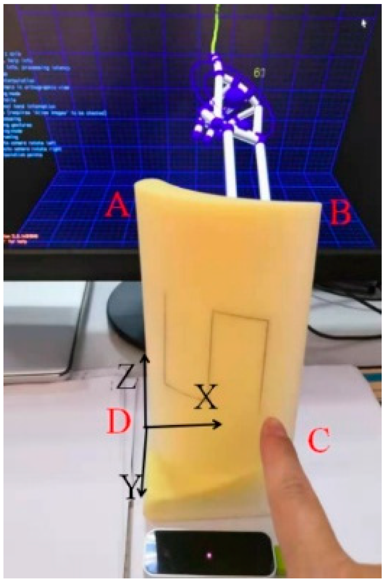
On the surface of the aircraft engine blade model, a Cartesian coordinate system defined by the X, Y, and Z axes is established. With reference to point D (X_D, Y_D, Z_D), four characteristic points on the model surface, namely A (X_A, Y_A, Z_A), B (X_B, Y_B, Z_D), C (X_D, Y_D, Z_D), and D (X_D, Y_D, Z_D), are selected. The Cartesian coordinates of the corresponding gesture points A, B, C, and D are transformed into the robot coordinate system according to Equation (1).

$$\left\{\begin{array}{c}{X}_t=-{\displaystyle \frac{Z_A-Z_D}{Z_{tA}-Z_{tD}}}{Z}_i+{\mathrm{X}}_D\\ \begin{array}{l}{Y}_t=-{\displaystyle \frac{Y_A-Y_C}{Y_{tA}-Y_{tC}}}{Y}_i+Y_D\\ Z_t={\displaystyle \frac{X_A-X_B}{X_{tA}-X_{tB}}}{X}_i+Z_D\end{array}\end{array}\right.$$

(1)

where X_i, Y_i, and Z_i are gesture coordinates, X_tA, Y_tB, and Z_tC are gesture coordinates, and X_t, Y_t, and Z_t are robot coordinate space coordinates. The coordinate units are all in mm.

2.2. Preprocessing of Gesture Trajectories

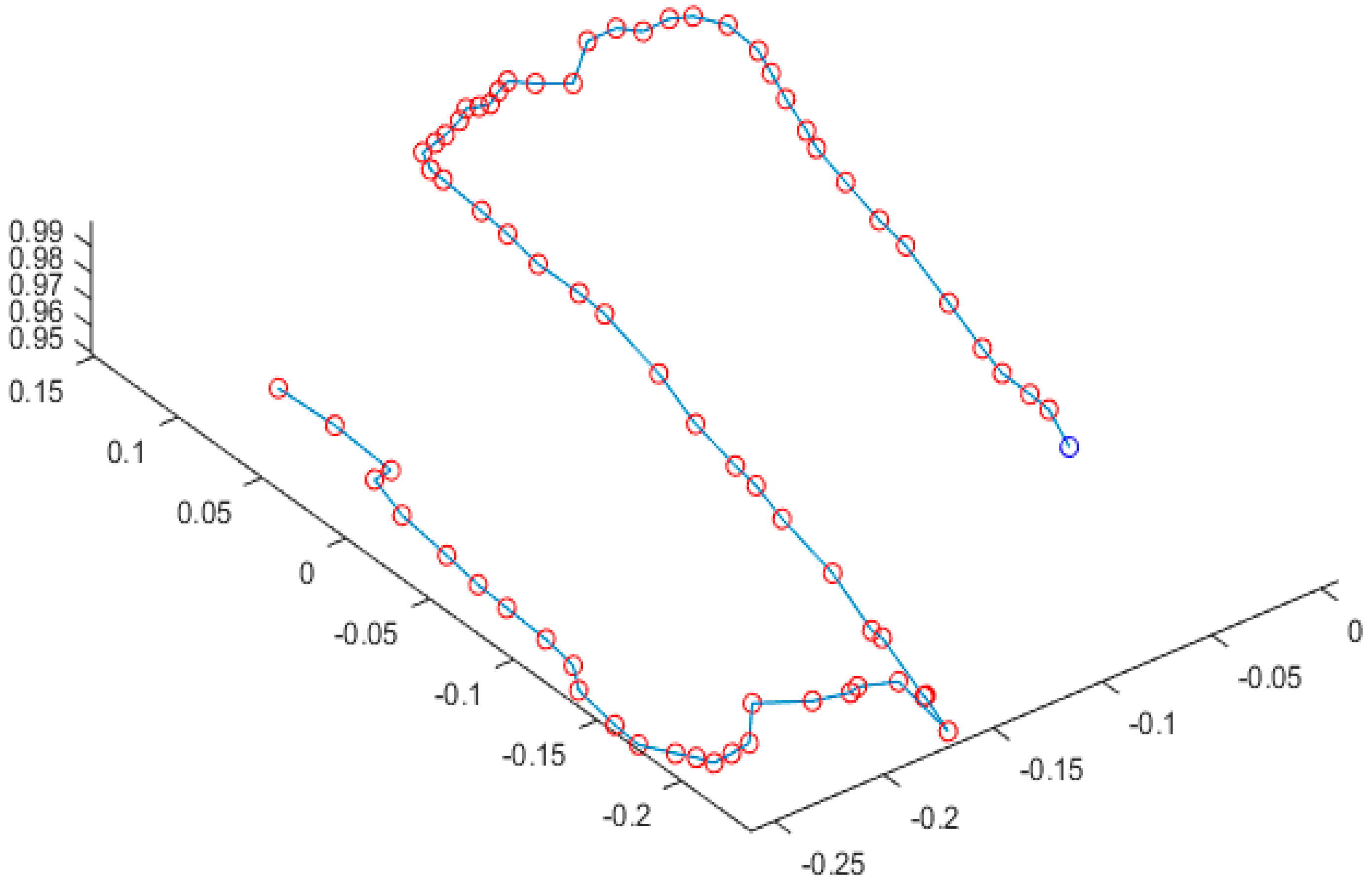
The complete gesture recognition process generally consists of gesture segmentation, tracking, recognition, and subsequent analysis and interpretation. Current research on human–machine interaction based on gesture recognition devices primarily focuses on gesture-to-action mapping for specific robotic tasks. After gesture acquisition, gesture interpretation and analysis are performed, followed by control feedback to realize human–robot interaction, gesture segmentation and recognition, and the execution of different robot actions based on matching results [4]. To investigate robot trajectory tracking based on gesture input, the coordinate information of fingertip trajectories traced along the target surface is extracted, yielding the gesture-derived trajectory shown in Figure 2. During surface tracing, slight finger vibrations can introduce positional offsets and measurement errors. Therefore, it is generally necessary to apply noise filtering to the gesture data to ensure accurate gesture-based robot control. With the advancement of robotic vision technologies, image information acquired by robots can be fed back to servo controllers, enabling online modification of the original trajectory and facilitating the accurate reproduction of complex trajectories.

This research used median filtering and mean filtering to smooth the initial trajectory, as shown in Equations (2) and (3).

$$g(x,y,z)=med\left\{f\right(x-k,y-l,z-m\left)\right\}$$

(2)

where k, l, and m are the three-dimensional coordinate range spaces in the x, y, and z directions, determined by the model. By taking the median or mean of five adjacent numbers on the three axes of each point, the optimal filtering under the minimum absolute error criterion can be obtained.

$$g(x,y,z)={\displaystyle \frac{\sum f(x,y,z)}{m}}$$

(3)

where m represents the spatial size, and the average value of the three-dimensional coordinate information f(x, y, z) is calculated. Process (3) to obtain the original data as shown in Figure 3.

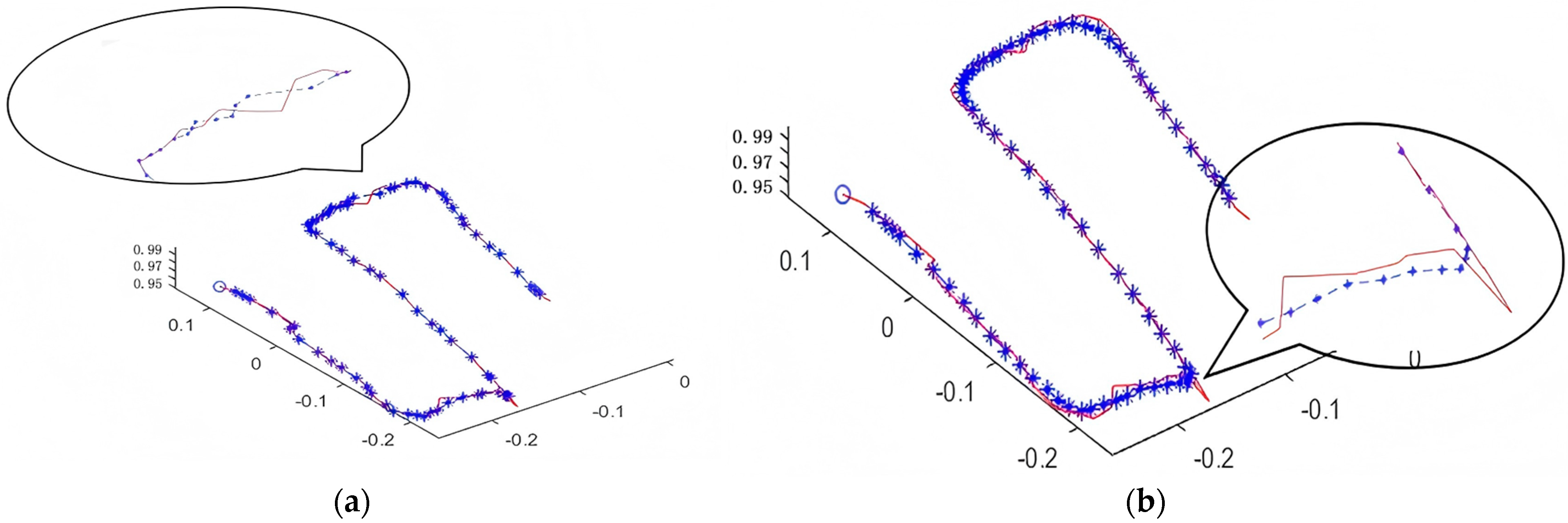
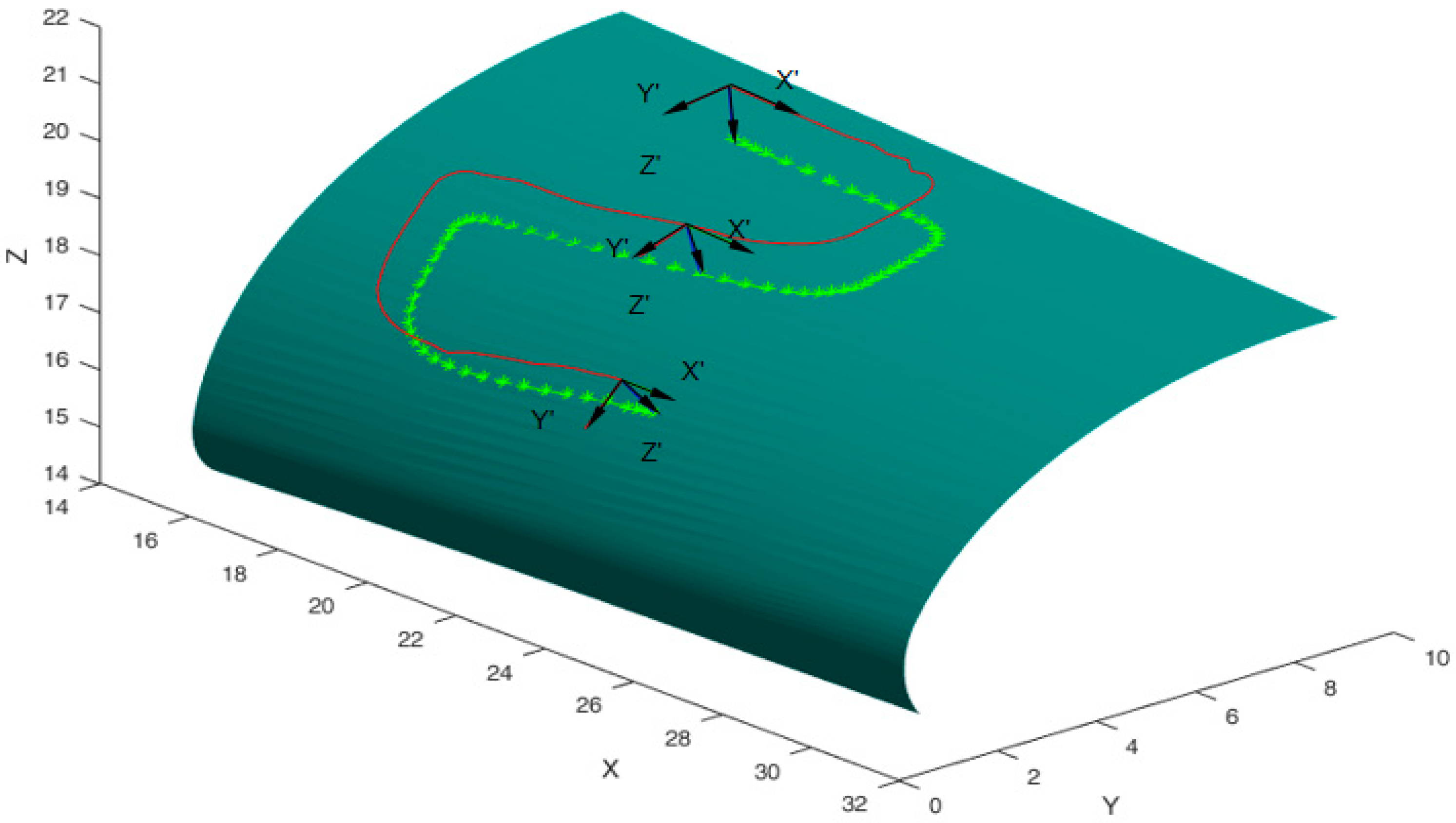
As shown in Figure 4, simple filtering tests demonstrate that median filtering can well preserve the original trajectory characteristics. Mean filtering exhibits stronger smoothing performance at inflection points; however, its overall trajectory matching accuracy at other regions is inferior to that of median filtering. In this research, mean filtering is applied to preprocess the gesture trajectories. After filtering, slight deviations in the trajectory data may still occur, causing certain scanning points to deviate from the actual surface of the inspected object. To eliminate preprocessing-induced errors, the normal projection of each scanning point is calculated based on the CAD model of the inspected object [26,27]. The corrected coordinates are then extended outward by 10 mm along the surface normal direction to obtain the corresponding robot coordinate-space path and robot pose at each trajectory point, as illustrated in Figure 4. After extension along the normal direction, the robot posture and the minimum distance to the surface remain unchanged, and the pose trajectory is subsequently planned accordingly.

2.3. Obtaining the Pose Matrix of Detection Points Based on Gesture Trajectory

Optimal trajectory planning in joint space requires determining the six-axis joint angles through the inverse kinematic solution of the pose matrices corresponding to the detection points. Subsequently, 5-5-5 spline polynomial interpolation is performed based on the joint angles at each detection point to generate smooth joint motion profiles. According to the CAD model surface geometry and its corresponding normal vectors, the scanning posture of the ultrasonic probe at each detection point is computed. The probe orientation is expressed using a direction cosine matrix to ensure that the emitted ultrasonic waves remain normal to the incident surface.

$$\{\begin{array}{c}{}_1{}^{0}T=rot(z_1,{\theta }_1)=\left[\begin{array}{cc}cos{\theta }_1& \begin{array}{ccc}-sin{\theta }_1& 0& 0\end{array}\\ \begin{array}{c}sin{\theta }_1\\ 0\\ 0\end{array}& \begin{array}{ccc}\begin{array}{c}cos{\theta }_1\\ 0\\ 0\end{array}& \begin{array}{c}0\\ 1\\ 0\end{array}& \begin{array}{c}0\\ 0\\ 1\end{array}\end{array}\end{array}\right]\\ {}_2{}^{1}T=rot(x_1,{90}^{°})trans(x_1,100)trans(y_2,100)rot(z_2,{\theta }_2)=\left[\begin{array}{cc}cos{\theta }_2& \begin{array}{ccc}-sin{\theta }_2& 0& 100\end{array}\\ \begin{array}{c}0\\ sin{\theta }_2\\ 0\end{array}& \begin{array}{ccc}\begin{array}{c}0\\ cos{\theta }_2\\ 0\end{array}& \begin{array}{c}-1\\ 1\\ 0\end{array}& \begin{array}{c}0\\ 100\\ 1\end{array}\end{array}\end{array}\right]\\ \begin{array}{c}{}_3{}^{2}T=trans(y_2,250)rot(z_4,{\theta }_4)=\left[\begin{array}{cc}cos{\theta }_3& \begin{array}{ccc}-sin{\theta }_3& 0& 250\end{array}\\ \begin{array}{c}sin{\theta }_3\\ 0\\ 0\end{array}& \begin{array}{ccc}\begin{array}{c}cos{\theta }_3\\ 0\\ 0\end{array}& \begin{array}{c}0\\ 1\\ 0\end{array}& \begin{array}{c}0\\ 0\\ 1\end{array}\end{array}\end{array}\right]\\ {}_4{}^{3}T=rot(y_3,{90}^{°})rot(z_4,{\theta }_4)=\left[\begin{array}{cc}0& \begin{array}{ccc}0& 1& 0\end{array}\\ \begin{array}{c}sin{\theta }_4\\ -cos{\theta }_4\\ 0\end{array}& \begin{array}{ccc}\begin{array}{c}cos{\theta }_4\\ sin{\theta }_4\\ 0\end{array}& \begin{array}{c}0\\ 0\\ 0\end{array}& \begin{array}{c}0\\ 0\\ 1\end{array}\end{array}\end{array}\right]\\ \begin{array}{c}{}_5{}^{4}T=rot(y_4,{-90}^{°})trans(x_4,250)rot(z_5,{\theta }_5)=\left[\begin{array}{cc}0& \begin{array}{ccc}0& -1& 0\end{array}\\ \begin{array}{c}sin{\theta }_4\\ cos{\theta }_5\\ 0\end{array}& \begin{array}{ccc}\begin{array}{c}cos{\theta }_4\\ -sin{\theta }_4\\ 0\end{array}& \begin{array}{c}0\\ 0\\ 0\end{array}& \begin{array}{c}0\\ 250\\ 1\end{array}\end{array}\end{array}\right]\\ {}_6{}^{5}T=rot(x_5,{90}^{°})rot(z_6,{\theta }_6)=\left[\begin{array}{cc}cos{\theta }_6& \begin{array}{ccc}-sin{\theta }_6& 0& 0\end{array}\\ \begin{array}{c}0\\ sin{\theta }_6\\ 0\end{array}& \begin{array}{ccc}\begin{array}{c}0\\ cos{\theta }_6\\ 0\end{array}& \begin{array}{c}-1\\ 0\\ 0\end{array}& \begin{array}{c}0\\ 0\\ 1\end{array}\end{array}\end{array}\right]\\ {}_6{}^{0}T=\left[\begin{array}{cc}{n}_x& \begin{array}{ccc}{o}_x& {\alpha }_x& p_x\end{array}\\ \begin{array}{c}{n}_y\\ n_z\\ 0\end{array}& \begin{array}{ccc}\begin{array}{c}{o}_y\\ o_z\\ 0\end{array}& \begin{array}{c}{\alpha }_y\\ {\alpha }_z\\ 0\end{array}& \begin{array}{c}{p}_y\\ p_z\\ 1\end{array}\end{array}\end{array}\right]\end{array}\end{array}\end{array}$$

(4)

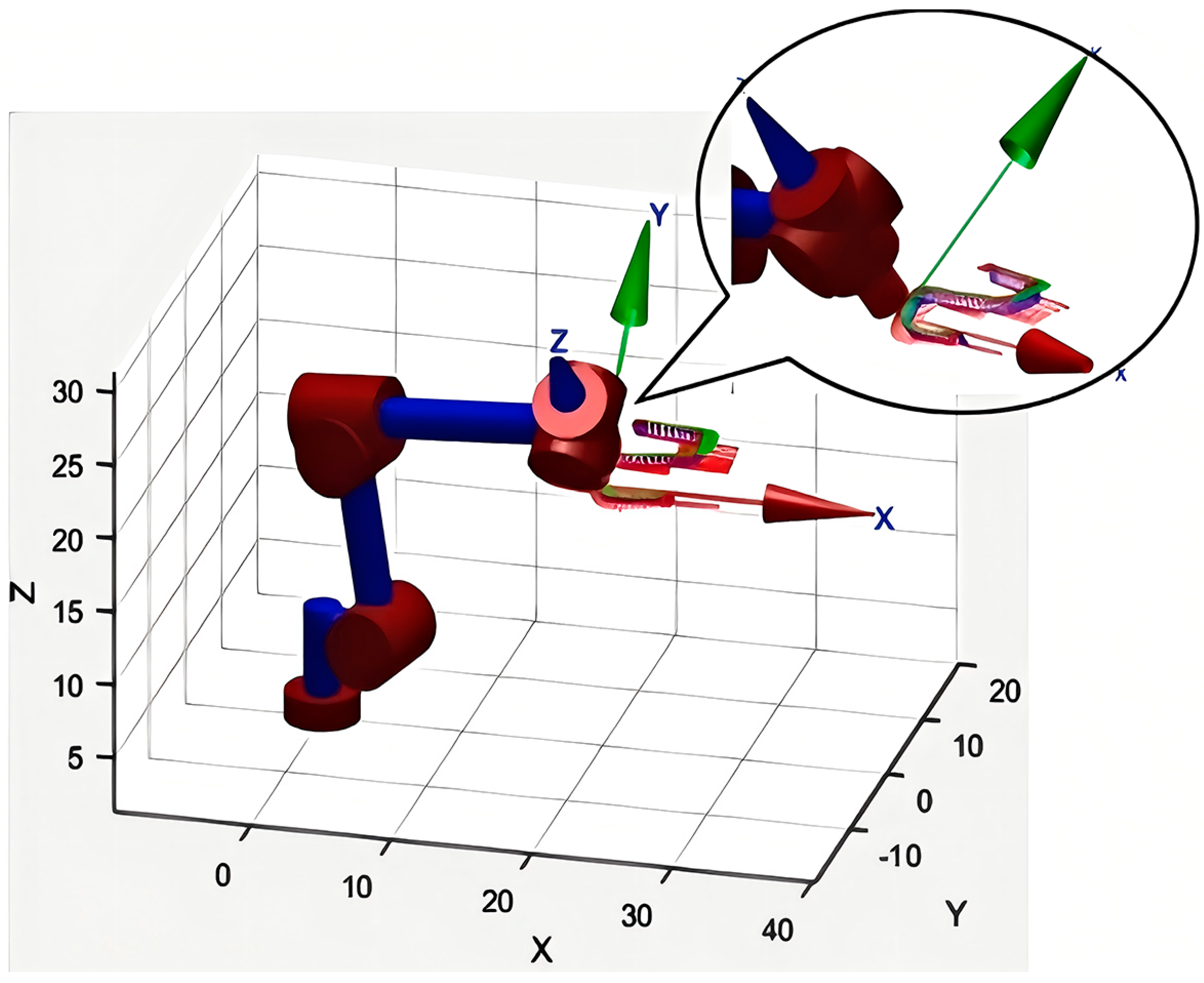
Specifically, the y-axis orientation remains unchanged, while the negative z-axis is aligned to be perpendicular to the surface. Establish a right-hand coordinate system as $\stackrel{⃑}{n}\times \stackrel{⃑}{x}=0$, $\stackrel{⃑}{n}\times \stackrel{⃑}{y}=0$, $\stackrel{⃑}{\tau }\times \stackrel{⃑}{z}=0$, where $\stackrel{⃑}{n}$ is the unit vector of the normal on the corresponding trajectory point on the surface, $\stackrel{⃑}{\tau }$ is the tangent unit vector of the corresponding trajectory point on the surface, and $\stackrel{⃑}{x},\stackrel{⃑}{y},\stackrel{⃑}{z}$ are the coordinate system unit vectors corresponding to the end of the robotic hand. At this point, the pose of the end effector of the robotic arm has not been determined, so the fixed unit vector $\stackrel{⃑}{y}$ is fixed relative to the X-axis of the world coordinate system, that is, in $\stackrel{⃑}{y}=\left[y_x{y}_y{y}_z\right]$, y_x is 0. The pose matrix is determined based on the direction cosine, and its starting, middle, and ending pose matrices are described in Equations (5)–(7). The first axis of the six axis joint angles corresponding to the detection point pose is shown in

Table 1. Six axis angles corresponding to pose matrix of detection point.

	J1	J2	J3	J4	J5	J6
T1	−0.1723	−0.2423	0.3839	0.7305	−0.2375	0.03496
Tmid	0.01786	−0.0450	0.3347	0.4002	−0.2825	−0.1281
Tend	0.2689	−0.0955	0.4786	0.1467	−0.3921	−0.3213

. The robot pose simulation during operation is shown in Figure 5.

The elements in the matrix are shown in Equation (5), where c_i represents cosθ_i and s_i represents sinθ_i.

$$\{\begin{array}{c}{n}_x={cos\theta }_6\left({cos}_5\left({cos}_1{c}_2{c}_3-c_1{s}_2{s}_3\right)+s_5\left(s_1{s}_4-c_4\left(c_1{c}_2{s}_3+c_1{c}_3{s}_2\right)\right)\right)+s_6\left(s_4\left(c_1{c}_2{s}_3+c_1{c}_3{s}_2\right){+c_{4}s}_1\right)\\ n_y=c_6\left(c_5\left(c_2{c}_3{s}_1-s_1{s}_2{s}_3\right)-s_5\left(c_1{s}_4-c_4\left(c_2{s}_1{s}_3+c_3{s}_1{s}_2\right)\right)\right)+s_6\left(s_4\left(c_2{s}_1{s}_3-c_3{s}_1{s}_2\right){+c_{1}s}_4\right)\\ \begin{array}{c}{n}_z=c_6\left(c_5\left(c_2{s}_3-c_3{s}_2\right)+{c_{4}s}_5\left(c_2{s}_3-{s_{2}s}_3\right)\right)-{s_{4}s}_6\left(c_2{s}_3-{s_{2}s}_3\right)\\ o_x={-s}_6\left(c_5\left(c_1{c}_2{c}_3-c_1{s}_2{s}_3\right)+s_5\left(s_1{s}_4-c_4\left(c_1{c}_2{s}_3+c_1{c}_3{s}_2\right)\right)\right)+s_6\left(s_4\left(c_1{c}_2{c}_3+c_1{c}_3{s}_2\right){+c_{4}s}_1\right)\\ \begin{array}{c}{o}_y=s_6\left(c_5\left(c_2{c}_3{s}_1-s_1{s}_2{s}_3\right)-s_5\left(c_1{s}_4-c_4\left(c_2{s}_1{s}_3+c_3{s}_1{s}_2\right)\right)\right)+s_6\left(s_4\left(c_2{s}_1{s}_3+c_3{s}_1{s}_2\right){-c_{1}s}_4\right)\\ o_z=-s_6\left(c_5\left(c_2{c}_3+c_3{s}_2\right)+{c_{4}s}_5\left(c_2{c}_3-{s_{2}s}_3\right)\right)-{s_{4}s}_6\left(c_2{c}_3-{s_{2}s}_3\right)\\ \begin{array}{c}{\alpha }_x=s_5\left(c_1{c}_2{c}_3-c_1{s}_2{s}_3\right)-c_5(s_1{s}_4-c_4\left(c_1{c}_2{s}_3+c_1{c}_3{s}_2\right))\\ n_y=s_5\left(c_2{c}_3{s}_1-s_1{s}_2{s}_3\right)+c_5(c_1{s}_4+c_4\left(c_2{s}_1{s}_3+c_3{s}_1{s}_2\right))\\ \begin{array}{c}{n}_z=s_5\left(c_2{s}_3+c_3{s}_2\right)-{c_{4}s}_5\left(c_2{c}_3-{s_{2}s}_3\right)\\ p_x=250c_1{s}_2{s}_3-250c_1{c}_2{c}_3-250c_1{s}_2+100\\ \begin{array}{c}{p}_y=100s_1-250s_1{s}_2-250c_2{c}_3{s}_1+250c_1{s}_2{s}_3\\ p_z=250c_2-250c_2{c}_3-250c_3{s}_2+100\end{array}\end{array}\end{array}\end{array}\end{array}\end{array}$$

(5)

$$T_1=\left[\begin{array}{cccc}0.9998& 0& 0.0176& 246.7182\\ 0.0116& 0.7500& -0.6614& 9.7164\\ -0.0132& 0.6615& 0.7498& 186.4363\\ 0& 0& 0& 1\end{array}\right]$$

(6)

$$T_{\mathit{mid}}=\left[\begin{array}{cccc}0.9998& 0& 0.0212& 216.4825\\ 0.0079& 0.9275& -0.3738& 33.8021\\ -0.0197& 0.3739& 0.9273& 201.3502\\ 0& 0& 0& 1\end{array}\right]$$

(7)

$$T_{\mathit{end}}=\left[\begin{array}{cccc}0.9988& 0& 0.0481& 205.9462\\ 0.0061& 0.9919& 0.1268& 67.9638\\ -0.0477& 0.1270& 0.9908& 211.1270\\ 0& 0& 0& 1\end{array}\right]$$

(8)

3. Joint-Space Continuous Trajectory Optimization

3.1. Continuous Trajectory Optimization Modeling

Robots are often required to execute repetitive and high-efficiency trajectory tasks, or motion tasks characterized by long execution times and significant dynamic impact. Consequently, optimizing robot motion trajectories to obtain smooth, well-conditioned trajectories is essential. During high-speed operation, joint friction and dynamic impact can reduce robot service life and degrade motion accuracy. Time–impact trajectory optimization is therefore necessary to mitigate these adverse effects and improve overall motion performance. In this research, polynomial interpolation, cubic spline interpolation, and cubic B-spline curve fitting are applied to the detection points, yielding robot trajectories with relatively smooth acceleration profiles. For continuous trajectory optimization, a non-contact ultrasonic scanning trajectory is planned to avoid scanning distance errors introduced by trajectory optimization. First, the surface trajectory is preprocessed based on the CAD model to eliminate geometric errors, and detection points are allocated along the trajectory. Subsequently, the scanning distance is increased along the surface’s normal direction while maintaining a constant offset. The scanning position trajectory is then optimized after distance extension. The resulting optimized trajectory satisfies the scanning requirements at all detection points and exhibits smooth velocity and acceleration characteristics during robot motion.

(1) Polynomial. Polynomial interpolation refers to determining a polynomial function that passes exactly through a given set of data points, as expressed in Equation (9). A polynomial of degree k guarantees continuity of the (k − 1)th derivative at the interpolation points, where the first-, second-, and third-order derivatives correspond to continuous velocity, continuous acceleration, and continuous jerk, respectively. When polynomial interpolation is applied in Cartesian space to fit a trajectory, fitting errors may arise. Moreover, although higher-order polynomials ensure continuity of velocity and acceleration, their fitting performance tends to deteriorate as the complexity and number of trajectory points increase.

$$p_i\left(x\right)=a_{ni}{x}^n+a_{(n-1)i}{x}^{n-1}+\dots +a_{2i}{x}^2+a_{1i}{x}^1+a_{0i}$$

(9)

The accuracy requirements of ultrasonic scanning points impose the constraint that the distance between the detection point position and the ultrasonic incidence point on the surface must remain constant. As the fitting accuracy deteriorates, data points located at the same nominal distance exhibit trajectory deviations. To mitigate these errors, the detection point positions can be corrected by computing the distance between the planned trajectory and the surface geometry.

(2) Cubic spline interpolation. Combining the piecewise functions of multiple cubic polynomials is called a cubic spline function. The cubic spline function curve is a piecewise cubic spline function within the range of $x_i\le x\le x_{i+1}$, where the first and second derivatives of the cubic polynomial in each segment are continuous, that is, the velocity and acceleration of the combined curve are continuous, as shown in Equation (10).

$$g_i\left(x\right)=a_i+b_i(x-x_i)+c_i(x-x_i{)}^2+d_i(x-x_i{)}^3$$

(10)

(3) Arc interpolation. Arc spline interpolation can be categorized into single-arc, double-arc, and triple-arc formulations. A single-arc spline inserts one circular arc segment at each interpolation point. Although a circular arc can be uniquely determined by two points and the tangent direction at one point, its stability is relatively poor; changes in the initial tangent direction require modification of the entire curve. Double-arc splines exhibit improved stability and provide limited capability for regulating curve shape. However, they ensure only G₁ continuity at the interpolation points, meaning that velocity continuity is achieved while curvature continuity is not. Triple-arc splines are constructed by connecting three arc segments end to end, with continuous tangent vectors between adjacent arcs. As a result, curvature continuity is satisfied at the interpolation points. The mathematical formulations of the single-arc, double-arc, and triple-arc splines are given in Equations (11)–(13).

Single arc spline. The midpoints of the curve are all three noncollinear points in space. For each point P_i (the position of the i-th point) passed, an arc is made to make adjacent arcs tangent, resulting in a G₁ continuous curve.

$$\{\begin{array}{c}\Vert O_i-O_{i+1}\Vert =\left|r_i+fla{g}_i\times r_{i+1}\right|,i=0,1,\dots 2n-1\\ \Vert O_i-P_{i+1}\Vert =r_i, \hspace{1em}\hspace{1em}\hspace{1em}\hspace{1em}\hspace{1em}i=0,1,\dots 2n-1\end{array}$$

(11)

where P_i is the type value point, r_i is the radius of the arc, O_i is the center of the circle, and flag represents the tangent of the arc. The arc is determined by the two type value points and the tangent vector.

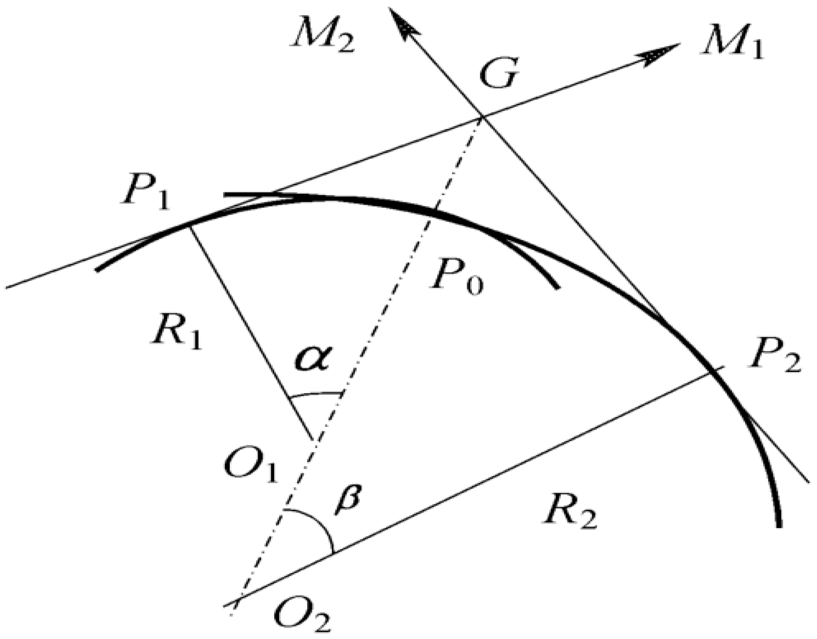
Double arc spline. Given two spatial points and their corresponding unit tangent vectors, two circular arc segments are constructed such that each arc is tangent to the specified tangent vector at its respective point, and the two arcs are mutually tangent to each other. Under these conditions, the formulation given in Equation (12) can be derived [26].

$$\{\begin{array}{c}G{P}_{i+1}\tan {\displaystyle \frac{{\beta }_{i+1}}{2}}=G{P}_i\tan {\displaystyle \frac{a_{i+1}}{2}}\\ a_i+{\beta }_{i+1}=180°-\angle P_{i}G{P}_{i+1}\end{array}$$

(12)

where GP_i is the distance from the intersection point of the tangent lines between the type value point and adjacent type value points, as shown in Figure 6. It is calculated together with $\angle P_{i}G{P}_{i+1}$ through the derivative at the type value point to determine the trajectory of the two arcs.

Cubic spline curve. By using two trajectory points, corresponding tangent vectors, and the center of the curvature circle, a cubic spline curve can be established, expressed in NURBS curve form as shown in (13) [26]:

$$T(t)={\displaystyle \frac{{\displaystyle \sum _{i=0}^6}{N}_{i,p}\left(t\right)w_i{P}_i}{{\displaystyle \sum _{i=0}^6}{N}_{i,p}\left(t\right)w_i}},0\le t\le 1$$

(13)

In this research, only arc interpolation is adopted for continuous trajectory optimization. For ultrasonic scanning applications, the spacing between successive trajectory points is relatively small, and thus continuity of velocity is the primary consideration. Accordingly, a single arc spline is employed to generate the optimized continuous trajectory.

(4) NURBS. In practical applications, NURBS curve or surface planning can be formulated in two ways: determining points on a curve or surface given known control points (the forward problem), or identifying the control points of a curve or surface from known shape points (the inverse problem). In this research, the inverse problem is addressed by interpolating a scanned point cloud to fit a NURBS curve. Specifically, the control points are reconstructed from the available shape points, and non-uniform rational B-spline interpolation is applied to the original point cloud data. The recursive formulation of the B-spline basis functions is given in Equation (14).

$$p(u)={\displaystyle \sum ^n}{d}_i{N}_{i}k\left(u\right)\begin{array}{c}\hspace{1em}\hspace{1em}i=0,1,2,\dots n\end{array}$$

(14)

where d_i is the control vertex, and continuous control vertices are connected to obtain a B-spline control polygon. $N_{i,k}\left(u\right)$ is the k-th B-spline basis function as shown in Equation (15), and $N_{i,0}\left(u\right)$ is shown in Equation (16).

$$N_{i,k}(u)={\displaystyle \frac{u-u_i}{u_{i+k}-u}}{N}_{i,k-1}(u)+{\displaystyle \frac{u_{i+k+1}-u}{u_{i+k+1}-u_{i+1}}}{N}_{i+1,k-1}(u)$$

(15)

$$N_{i,0}(u)=\{\begin{array}{cc}1\hfill & u_i\le u\le u_{i+1}\hfill \\ 0\hfill & another\hfill \end{array}$$

(16)

3.2. Continuous Trajectory Optimization of Joint-Space Surfaces

Surface multi-trajectory point control can be realized using point-to-point trajectory control methods with continuous interpolation and combination; however, this approach is computationally intensive and inefficient. In this research, impact optimization is omitted in the continuous multi-trajectory point optimization process. Instead, cubic spline interpolation, B-spline interpolation, and arc interpolation are employed to interpolate robot joint-space trajectory points and generate optimized motion trajectories. Based on the velocity and acceleration characteristics of the trajectories, the time intervals between successive trajectory points are adaptively adjusted to achieve a reduction in the acceleration at each trajectory point.

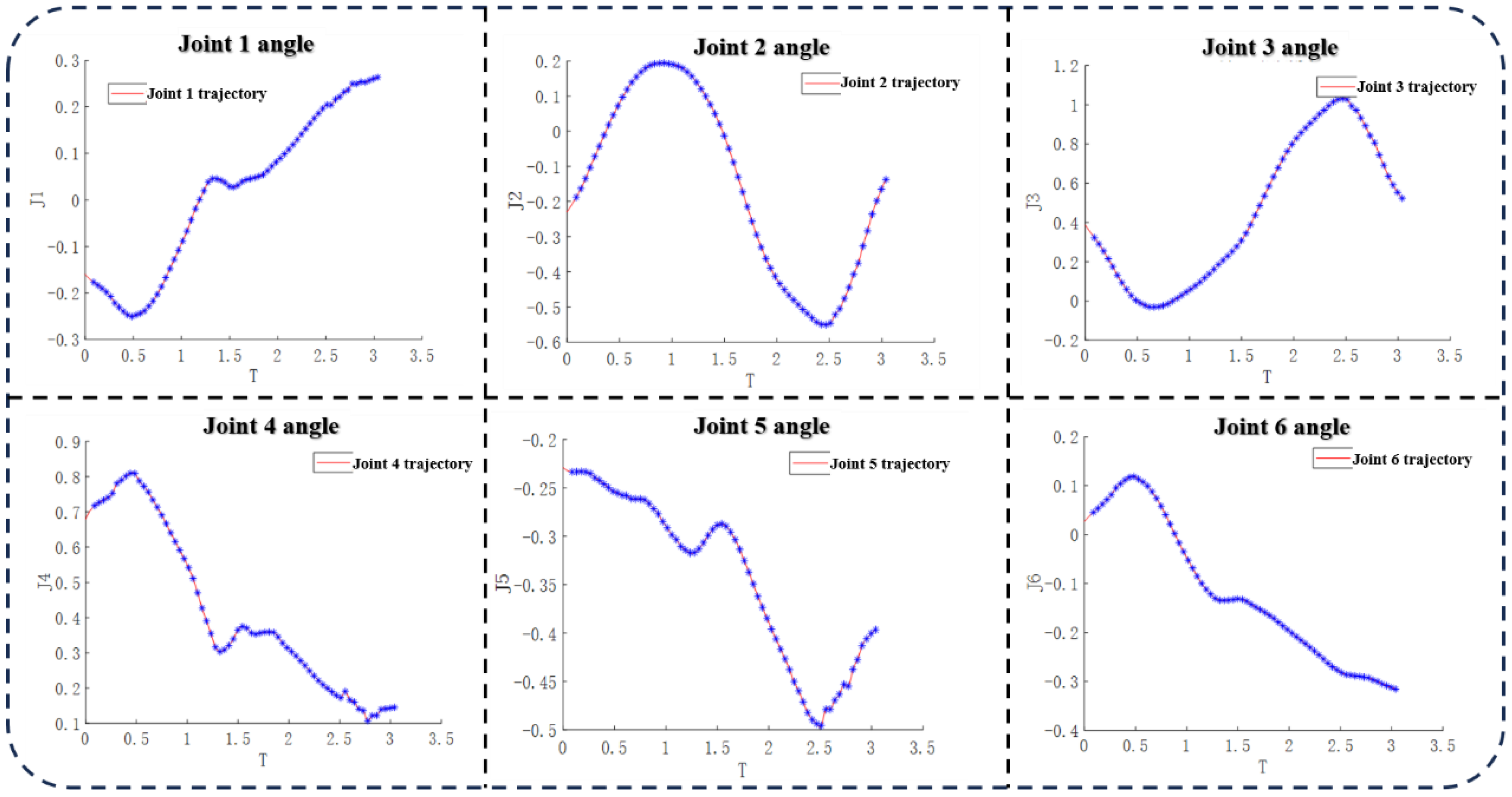
(1) Cubic spline interpolation. Cubic spline interpolation represents a curve composed of multiple cubic polynomial segments. At the junctions between adjacent spline segments, continuity G₀, G₁, and G₂ is ensured, corresponding to the continuity of position, velocity, and acceleration, as expressed in Equation (10). By means of differential coefficients, this method enables control of the maximum angular velocity and maximum angular acceleration of the trajectory. Under the constraints of allowable angular velocity and acceleration, the robot motion parameters are computed, the time intervals between trajectory points are allocated, and the acceleration profile is optimized. Consequently, time information is embedded into the joint-space trajectory points. As shown in Figure 7, the optimized cubic spline trajectories are obtained through interpolation of the trajectory points in each joint space.

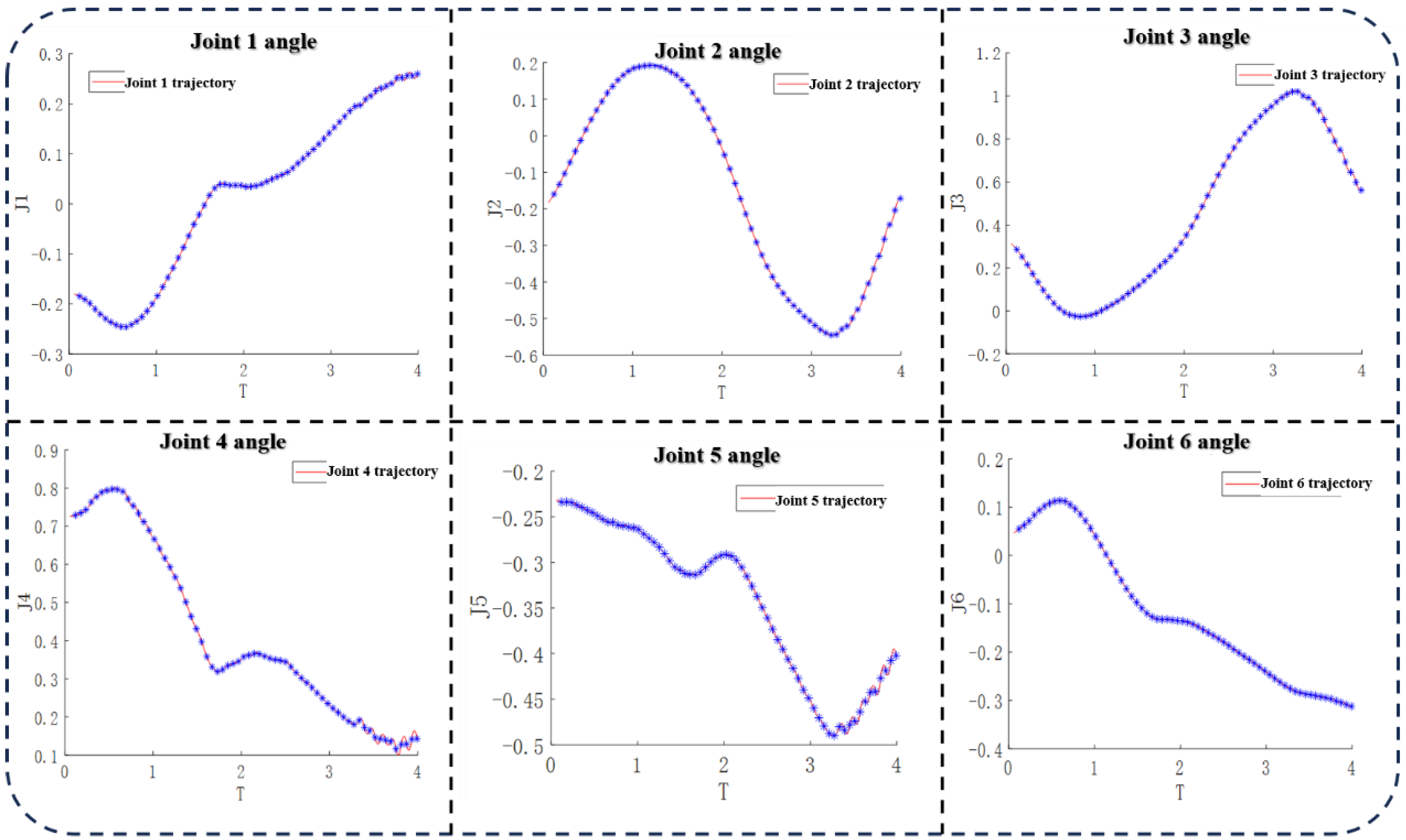
(2) Arc spline interpolation. Arc spline interpolation constructs a motion trajectory by inserting multiple circular arc segments between successive trajectory points. Taking a single arc spline as an illustrative example, continuous interpolation optimization is applied to the joint-space trajectory points of the robot during ultrasonic scanning. The tangent direction at each trajectory point is first determined, and the total number of arc segments in the spline is governed by the number of trajectory points. At the junctions between adjacent trajectory points, continuity of velocity and acceleration is ensured through tangential continuity, as defined in Equation (11). The joint-space trajectory generated using single-arc interpolation is shown in Figure 8.

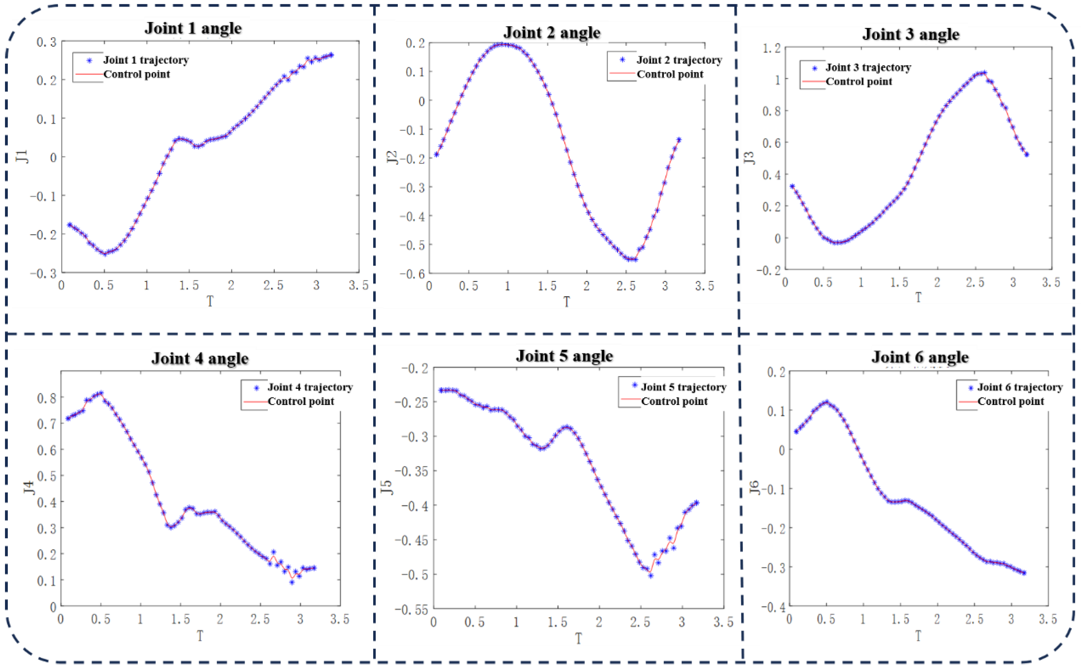
(3) NURBS. Non-uniform rational B-splines (NURBS) employ control vertices to define and manipulate curve geometry, and Equation (16) is used to interpolate and optimize the trajectories of the six-axis joints. In the present research, where the trajectory points are predefined, the control vertices are recursively computed using Equation (15), thereby generating the corresponding interpolation curve. By taking time as the independent variable and the six joint angle values as dependent variables, cubic B-spline interpolation is applied in joint space to optimize the robot trajectory, as illustrated in Figure 9.

3.3. Comparative Analysis of Three Continuous Trajectory Optimization Methods

Using cubic spline interpolation, B-spline interpolation, and arc interpolation, the trajectory points in the robot joint space were interpolated. Based on the maximum speed constraints of the Epson C3 robot produced by Epson Engineering (Shenzhen) Ltd in China listed in

Table 2. Epson C3 six-axis robot maximum speed constraint.

Joint	J1	J2	J3	J4	J5	J6
Maximum speed constraint (rad/s)	450π/180	450π/180	513π/180	555π/180	555π/180	720π/180

, the total motion time of the optimized trajectories for the three interpolation methods was obtained. By imposing maximum acceleration constraints, joint trajectories with explicit time information were generated. The motion times of the six joints were then normalized with respect to the longest joint motion time, allowing the trajectory duration, maximum angular velocity, and maximum angular acceleration for each method to be determined. Under these constraints, the corresponding maximum impact force was calculated. A comparative summary of the trajectory optimization results under the three interpolation schemes is presented in

Table 3. Continuous trajectory optimization of joint space under the constraint of maximum acceleration.

Trajectory Optimization Methods	Time (s)	Maximum Angular Velocity (rad/s)
Cubic spline interpolation	3.0393	1.1612
Single arc spline interpolation	3.9920	1.2368
NURBS interpolation	3.1701	1.0767

. The results indicate that, for continuous trajectories with a large number of trajectory points, cubic spline interpolation yields a shorter total motion time and a lower impact force than the other two methods.

As shown in Table 3, during the optimization of the gesture-based ultrasound scanning trajectory, for continuous trajectory optimization with a small spacing between trajectory points, the trajectory generated using cubic spline interpolation exhibits a shorter execution time, whereas the trajectory obtained via NURBS interpolation demonstrates a lower maximum angular velocity. The latter approach provides superior curve smoothness. Based on these findings, the joint-space trajectory is generated using the NURBS interpolation method, and the corresponding Cartesian-space trajectory is subsequently obtained through forward kinematics, as illustrated in Figure 10a. The resulting trajectory is then imported into the MATLAB R2023b Robotics Toolbox for simulation, yielding the robot motion trajectory shown in Figure 10b.

4. Optimization of Optimal Trajectory for Point-to-Point Impact in Joint Space

In point-to-point scanning trajectory planning for sampling-based inspection, increasing the scanning speed to reduce overall inspection time inevitably introduces impact forces during joint motion, which can lead to scanning point deviations and accelerate mechanical wear, thereby shortening the service life of the robot. Although Cartesian-space trajectory optimization can ensure smooth motion of the robot end effector, the resulting inter-joint impact forces remain difficult to regulate. To address this issue, a fifth-degree polynomial spline is employed to interpolate the inspection points. By imposing constraints on the maximum joint angular velocity, angular acceleration, and angular jerk, the impact forces induced during trajectory execution are effectively limited. A particle swarm optimization algorithm is then applied to search for a fifth-degree polynomial trajectory that satisfies the impact force constraints. After weighted optimization, an optimal time–impact trajectory is obtained.

4.1. A 5-5-5 Interpolation Polynomial

Time–impact optimal trajectory planning is performed for point-to-point motion to ensure accuracy, efficiency, and smoothness throughout the scanning process. A fifth-degree polynomial spline is adopted to interpolate the scanning curve. Fu et al. [10] employed 3-5-3 polynomial interpolation for time-optimal robot path planning; however, the associated formulation did not account for impact, which led to relatively large accelerations at the transition between adjacent time segments. In the present research, impact is explicitly incorporated into joint-space optimization, and a 5-5-5 interpolation scheme is constructed to optimize point-to-point trajectories. The use of fifth-degree polynomials ensures acceleration continuity at segment boundaries, thereby yielding smoother acceleration profiles along the entire trajectory. The polynomial expression is given as follows [6]:

$$X_{ij}=a_{i6}+a_{i5}{t}_j+a_{i4}{t_j}^2+a_{i3}{t_j}^3+a_{i2}{t_j}^4+a_{i1}{t_j}^5$$

(17)

$$X_{i2}=a_{i12}+a_{i11}{t}_2+a_{i10}{t_2}^2+a_{i9}{t_2}^3+a_{i8}{t_2}^4+a_{i7}{t_2}^5$$

(18)

$$X_{i3}=a_{i18}+a_{i17}{t}_3+a_{i16}{t_3}^2+a_{i15}{t_3}^3+a_{i14}{t_3}^4+a_{i13}{t_3}^5$$

(19)

In the formula, X_ij is the angle of the j-th segment of the i-th axis. For each time planning a point-to-point trajectory for four points, three fifth degree polynomials need to be obtained. When the starting and ending points are in a stopped state, the angle, angular velocity, and angular acceleration of the first and last points of the trajectory are 0. After knowing the path points X_i20 and X_i30, the polynomial coefficients are obtained by inputting them into three time periods t₁, t₂, and t₃. Based on the derivative function of the three fifth degree polynomials, the velocity during that period is calculated. Accelerations, according to the correspondence between the three fifth-degree polynomials and the time period, are shown in Equations (20)–(22) [6].

$$\mathrm{A}=\left[\begin{array}{cccccccccccccccccc}{{\mathrm{t}}_1}^5& {{\mathrm{t}}_1}^4& {{\mathrm{t}}_1}^3& {{\mathrm{t}}_1}^2& {{\mathrm{t}}_1}^1& 1& 0& 0& 0& 0& 0& 1& 0& 0& 0& 0& 0& 0\\ 5{{\mathrm{t}}_1}^4& 4{{\mathrm{t}}_1}^3& 3{{\mathrm{t}}_1}^2& 2{{\mathrm{t}}_1}^1& 1& 0& 0& 0& 0& 0& -1& 0& 0& 0& 0& 0& 0& 0\\ 20{{\mathrm{t}}_1}^3& 12{{\mathrm{t}}_1}^2& 6{{\mathrm{t}}_1}^1& 2& 0& 0& 0& 0& 0& -2& 0& 0& 0& 0& 0& 0& 0& 0\\ 60{{\mathrm{t}}_1}^2& 24{{\mathrm{t}}_1}^1& 6& 0& 0& 0& 0& 0& -6& 0& 0& 0& 0& 0& 0& 0& 0& 0\\ 0& 0& 0& 0& 0& 0& {{\mathrm{t}}_2}^5& {{\mathrm{t}}_2}^4& {{\mathrm{t}}_2}^3& {{\mathrm{t}}_2}^2& {{\mathrm{t}}_2}^1& 1& 0& 0& 0& 0& 0& -1\\ 0& 0& 0& 0& 0& 0& 5{{\mathrm{t}}_2}^4& 4{{\mathrm{t}}_2}^3& 3{{\mathrm{t}}_2}^2& 2{{\mathrm{t}}_2}^1& 1& 0& 0& 0& 0& 0& -1& 0\\ 0& 0& 0& 0& 0& 0& 20{{\mathrm{t}}_2}^3& 12{{\mathrm{t}}_2}^2& 6{{\mathrm{t}}_2}^1& 2& 0& 0& 0& 0& 0& -2& 0& 0\\ 0& 0& 0& 0& 0& 0& 60{{\mathrm{t}}_2}^2& 24{{\mathrm{t}}_2}^1& 6& 0& 0& 0& 0& 0& -6& 0& 0& 0\\ 0& 0& 0& 0& 0& 0& 0& 0& 0& 0& 0& 0& {{\mathrm{t}}_3}^1& {{\mathrm{t}}_3}^1& {{\mathrm{t}}_3}^1& {{\mathrm{t}}_3}^1& {{\mathrm{t}}_3}^1& 1\\ 0& 0& 0& 0& 0& 0& 0& 0& 0& 0& 0& 0& 5{{\mathrm{t}}_3}^1& 4{{\mathrm{t}}_3}^1& 3{{\mathrm{t}}_3}^1& 2{{\mathrm{t}}_3}^1& 1& 0\\ 0& 0& 0& 0& 0& 0& 0& 0& 0& 0& 0& 0& 20{{\mathrm{t}}_3}^1& 12{{\mathrm{t}}_3}^1& 6{{\mathrm{t}}_3}^1& 2& 0& 0\\ 0& 0& 0& 0& 0& 0& 0& 0& 0& 0& 0& 0& 60{{\mathrm{t}}_3}^1& 24{{\mathrm{t}}_3}^1& 6& 0& 0& 0\\ 0& 0& 0& 0& 0& 1& 0& 0& 0& 0& 0& 0& 0& 0& 0& 0& 0& 0\\ 0& 0& 0& 0& 1& 0& 0& 0& 0& 0& 0& 0& 0& 0& 0& 0& 0& 0\\ 0& 0& 0& 1& 0& 0& 0& 0& 0& 0& 0& 0& 0& 0& 0& 0& 0& 0\\ 0& 0& 1& 0& 0& 0& 0& 0& 0& 0& 0& 0& 0& 0& 0& 0& 0& 0\\ 0& 0& 0& 0& 0& 0& 0& 0& 0& 0& 0& 0& 0& 0& 0& 0& 0& 1\\ 0& 0& 0& 0& 0& 0& 0& 0& 0& 0& 0& 1& 0& 0& 0& 0& 0& 0\end{array}\right]$$

(20)

$$\mathrm{b}=\left[\begin{array}{cccc}\begin{array}{cccc}0& 0& 0& 0\end{array}& \begin{array}{cccc}0& 0& 0& 0\end{array}& \begin{array}{cccc}r3& 0& 0& 0\end{array}& \begin{array}{cccc}r0& v0& a0& \begin{array}{ccc}0& r2& r1\end{array}\end{array}\end{array}\right]$$

(21)

$$A\cdot a=b$$

(22)

To determine the maximum angular velocity along the trajectory, an S-shaped acceleration-deceleration profile is employed to construct polynomial splines for each set of four inspection points. For any two adjacent groups of inspection points, continuity constraints are imposed such that the joint angle, angular velocity, angular acceleration, and angular jerk at the initial and terminal points are identical, thereby ensuring smooth motion transitions and minimizing dynamic impact throughout the trajectory.

4.2. Impact-Optimal Trajectory Planning Based on Particle Swarm Optimization Algorithm

In studies on time–impact optimal trajectory planning, Gasparetto et al. [12] assigned weighting factors to two optimization objectives, execution time and impact, and converted the multi-objective problem into a single-objective formulation. By adjusting the weights at different stages, the optimization priority between time and impact was varied, ultimately achieving reduced execution time while maintaining low impact levels. Xiao et al. [27] similarly adopted time, acceleration, and impact as optimization objectives to perform hybrid optimal trajectory planning. In the present research, a particle swarm optimization (PSO) algorithm is employed to search for the coefficients of fifth-degree polynomials, which exhibit fewer local optima. For each inspection point, PSO is used to identify polynomial coefficients that minimize execution time while satisfying impact constraints. Specifically, the fitness value is constructed as a weighted combination of time and impact [28]. The process of continuously searching for the minimum execution time under acceleration constraints is formulated using two fitness functions: an objective function and a constraint function, as defined in Equations (22) and (23) [6].

$$f_1={\mathrm{W}}_t(t1+t2+t3)+{\mathrm{W}}_{\mathrm{j}}\cdot |j_{\max }-\max j|$$

(23)

$$f_2={\mathrm{W}}_t(*(t1+t2+t3)+W_j*\left|\max j\right|$$

(24)

where W is the weight, j is the acceleration, (23) finds the configuration with the closest acceleration to the constraint and less time, and (24) modifies the configuration that exceeds the constraint to optimize its particle swarm velocity in the direction of reducing the impact force, achieving the shortest time local optimal solution that meets the constraint conditions. The specific algorithm process is as follows:

(1) Initialize particles. Set the number and dimension of particles by taking three periods of time t as their positions.

(2) Calculate the acceleration of particles. Substitute three periods of time t into Equations (20)–(22) to obtain the coefficient vector a. Based on the obtained polynomial coefficients, apply them to Equations (17)–(19) to obtain the maximum acceleration of the three polynomial curves. Using Equation (23) as the fitness function, calculate the initial individual extremum p-best and the initial global extremum g-best.

(3) Calculate particle fitness. Determine whether the maximum acceleration of the global optimal solution exceeds the maximum constraint. If it does not exceed the acceleration constraint, calculate the fitness value using the fitness function in Equation (23), and iterate over three periods of time using Equations (1) and (2) to obtain new particles. If the acceleration constraint exceeds the maximum constraint, the fitness of the single dimensional particle over three time periods exceeding the maximum constraint is calculated using Equation (24) as the fitness function, and a new global optimal solution that satisfies the constraint is iteratively selected.

(4) Determine whether the termination condition has been met. If not, return step (2) and eventually converge to the solution space with a slightly lower acceleration than the maximum constraint.

4.3. Optimization of Point-to-Point Trajectories on Surfaces

Several representative points are selected on the surface, such as the four points listed in

Table 4. Select four points on the surface.

	X	Y	Z
A	24.6542	1.63295	17.8938
B	18.6055	3.1178	19.063
C	25.6276	5.72161	19.672
D	20.5465	6.92312	20.122

. Points A and D correspond to the start and end positions, respectively, with both joint velocity and acceleration set to zero. Points B and C represent the minimum and maximum positions of the surface along the X-axis in Figure 11. The inverse kinematics solutions for these four points are first computed, after which the corresponding trajectory points are optimized. By prescribing the joint angle, angular velocity, and angular acceleration at the four points as boundary conditions, three segments of fifth-degree polynomial curves are constructed. Taking zero velocity and acceleration at the initial and terminal points as constraints, trajectory optimization is performed with the objective of minimizing the total execution time.

During ultrasonic point scanning, the intermediate trajectories associated with non-target positions can be disregarded. To reduce overall trajectory execution time while limiting impact forces and thereby minimizing scanning errors, the trajectory is optimized by constraining the joint velocity, acceleration, and jerk at the corresponding trajectory points. Conventional interpolation methods, including polynomial interpolation, cubic spline interpolation, circular arc interpolation, and NURBS interpolation, provide limited flexibility in directly regulating trajectory acceleration profiles. Therefore, an improved GA-PSO hybrid algorithm is applied to the six-axis joints of the robot, subject to constraints of a maximum joint velocity of π rad/s, a maximum joint acceleration of 10 rad/s², and a maximum joint jerk of 50 rad/s³. The weighting ratio between execution time and impact is set to W_t:W_v = 3:7. The six joint axes and the three trajectory segments are jointly optimized to obtain the optimal execution time for each segment, as summarized in

Table 5. The optimal time interval under the constraint of four-point trajectory of six joints.

	J1	J2	J3	J4	J5	J6
t1 (s)	0.6538	1.1539	1.0208	0.7457	0.4598	0.5128
t2 (s)	0.3083	1.1516	1.0306	0.3933	0.5497	0.2615
t3 (s)	0.5189	1.7335	1.7839	0.4893	0.6690	0.7240

.

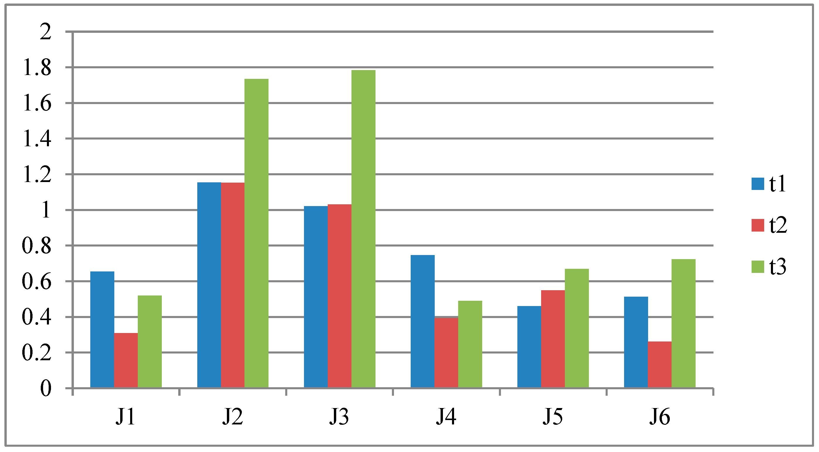
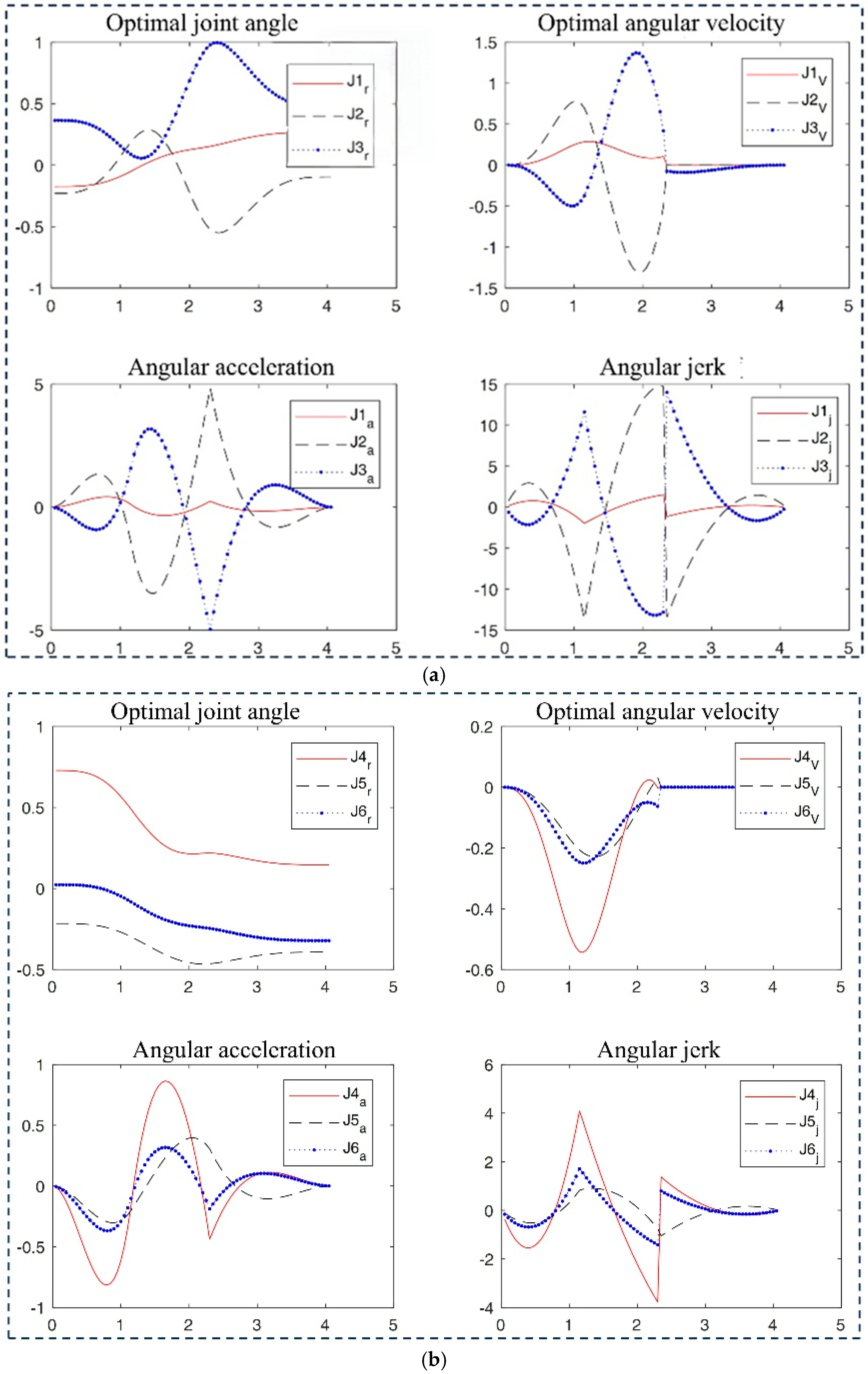
For each motion segment, the longest execution time among the six joint axes is selected, yielding three segment durations of 1.1539 s, 1.1516 s, and 1.7839 s, respectively, with a total execution time of 4.0894 s, as shown in Figure 12. Based on these segment durations, the joint angular velocity, angular acceleration, and angular jerk of the six joints are recalculated for each segment. The final results of the optimization iterations are illustrated in Figure 13, where the joint angles are expressed in radians. When extracting the trajectories of the four key trajectory points, particular attention must be paid to the acceleration and impact characteristics during interpolation. The effectiveness of the trajectory optimization is clearly demonstrated, and the corresponding maximum angular velocity, angular acceleration, and angular jerk are summarized in

Table 6. Maximum angular velocity, angular acceleration and angular jerk.

Point-to-Point Trajectory Optimization	Time (s)	Maximum Angular Velocity (rad/s)	Maximum Angular Acceleration (rad/s2)	Maximum Angular Jerk (rad/s3)
5-5-5 interpolation	4.0894 s	1.3707	4.8531	14.7562

.

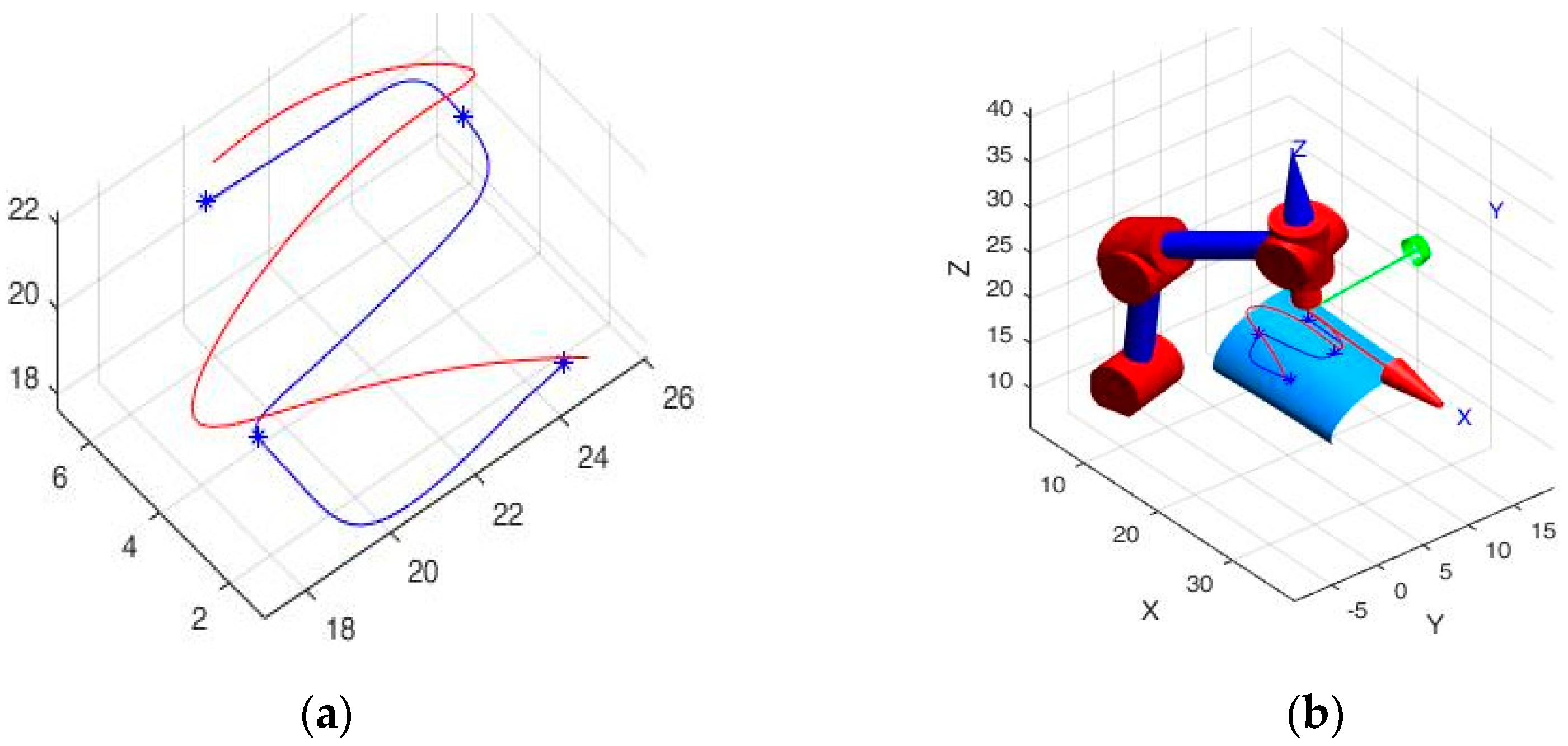
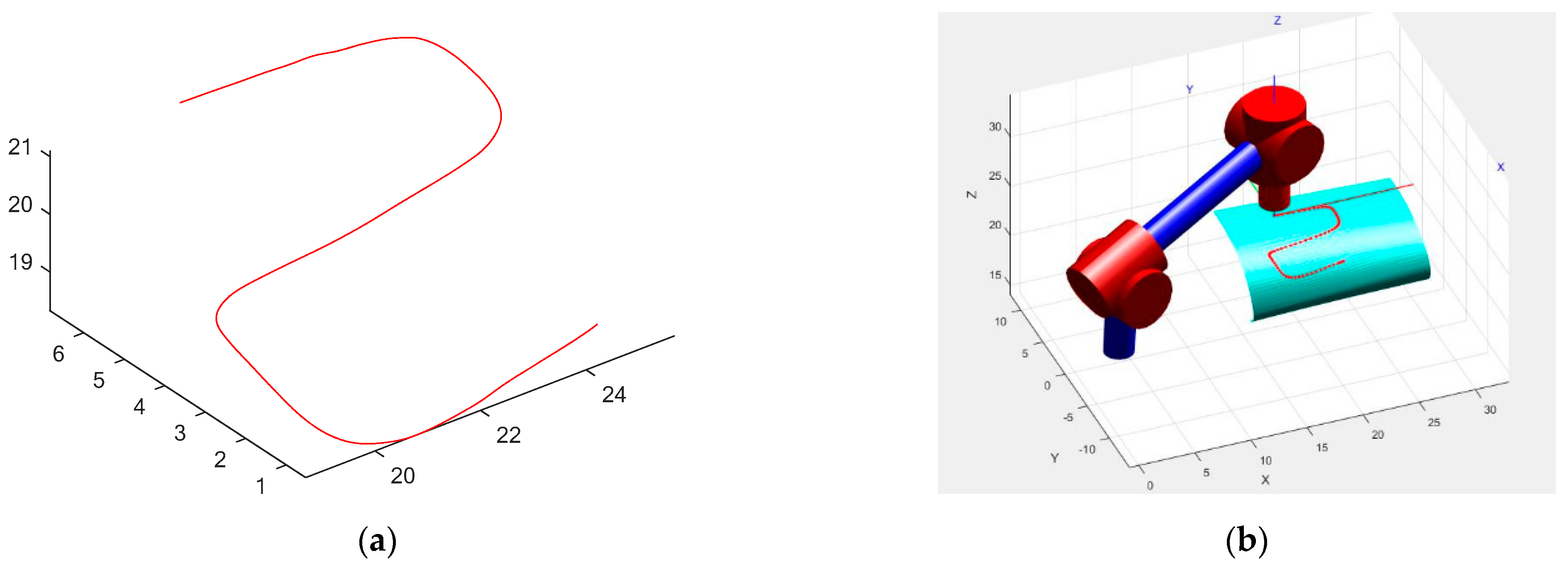
As shown in Figure 13, the velocities, accelerations, and jerks of all six axes remain within the prescribed constraints. The fourth axis exhibits no variation in angular motion, while a sudden change in acceleration is observed at the third key point; however, the corresponding jerk does not exceed 15 rad/s³, indicating a relatively low dynamic impact. By substituting the three optimal time intervals into Equations (15)–(17), the final trajectory of the six-axis robot in Cartesian space is obtained. The end-effector trajectory is illustrated in Figure 14. Specifically, Figure 14a shows the original pose trajectory of the robot end effector, which lies in a single plane. The red curve in Figure 14a represents the optimized trajectory with a surface impact depth of 10 mm, forming a spatial curve. The motion of this spatial trajectory is further simulated using the MATLAB Robotics Toolbox, and the corresponding results are presented in Figure 14b.

4.4. Experiment

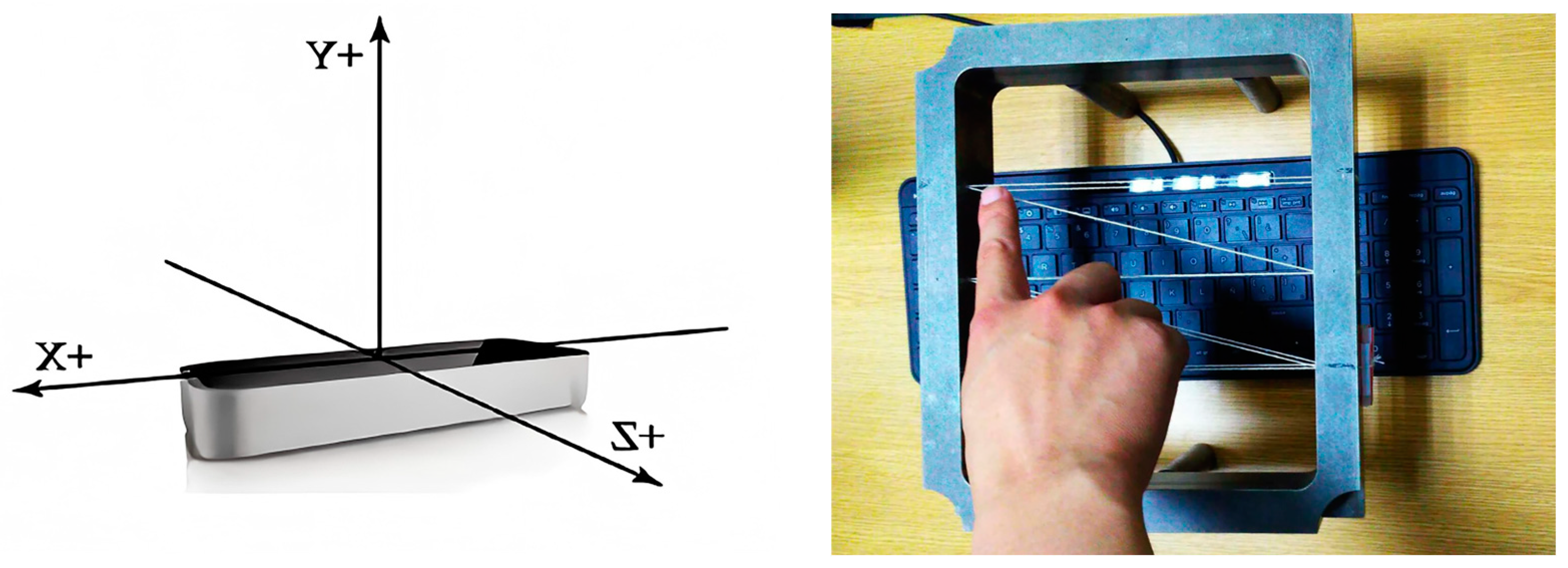
(1) Leap Motion gesture recognition device. Leap Motion employs infrared imaging and vision-based tracking technology to capture hand motion data. By means of infrared sensors and cameras, it tracks hands and fingers, or tools to acquire the spatial positions, gestures, and motion states of the detected objects. The system provides both static and dynamic interaction information to users, and its external structure and internal coordinate system are illustrated in Figure 15. Hand posture information is obtained by computing the spatial coordinates of the palm and fingers. However, when this posture acquisition method is applied to robotic interaction, it introduces inherent inaccuracies, particularly in trajectory planning tasks that require high-precision pose information for robotic end effectors.

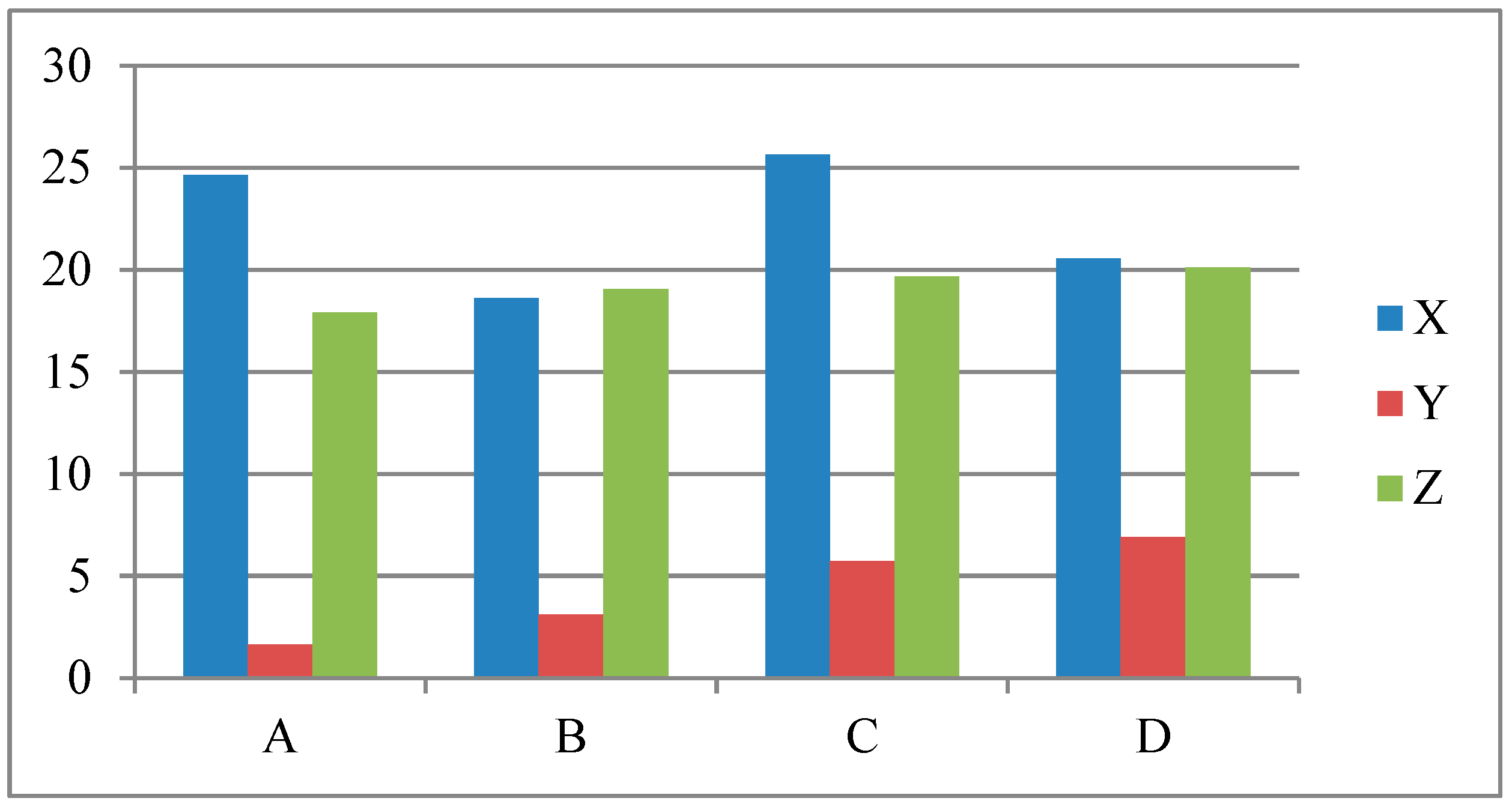
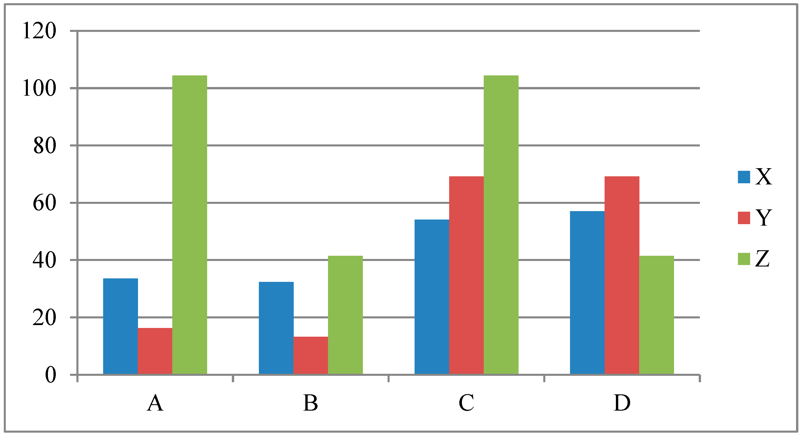
(2) Comparative analysis of experimental data. The obtained data is shown in

Table 7. ABCD four-point robot simulation space coordinates.

	X	Y	Z
A	33.5663	16.2312	104.4131
B	32.3663	13.2312	41.4131
C	54.0663	69.2312	104.4131
D	57.0663	69.23121	41.4131

.

And the variation pattern is shown in Figure 16.

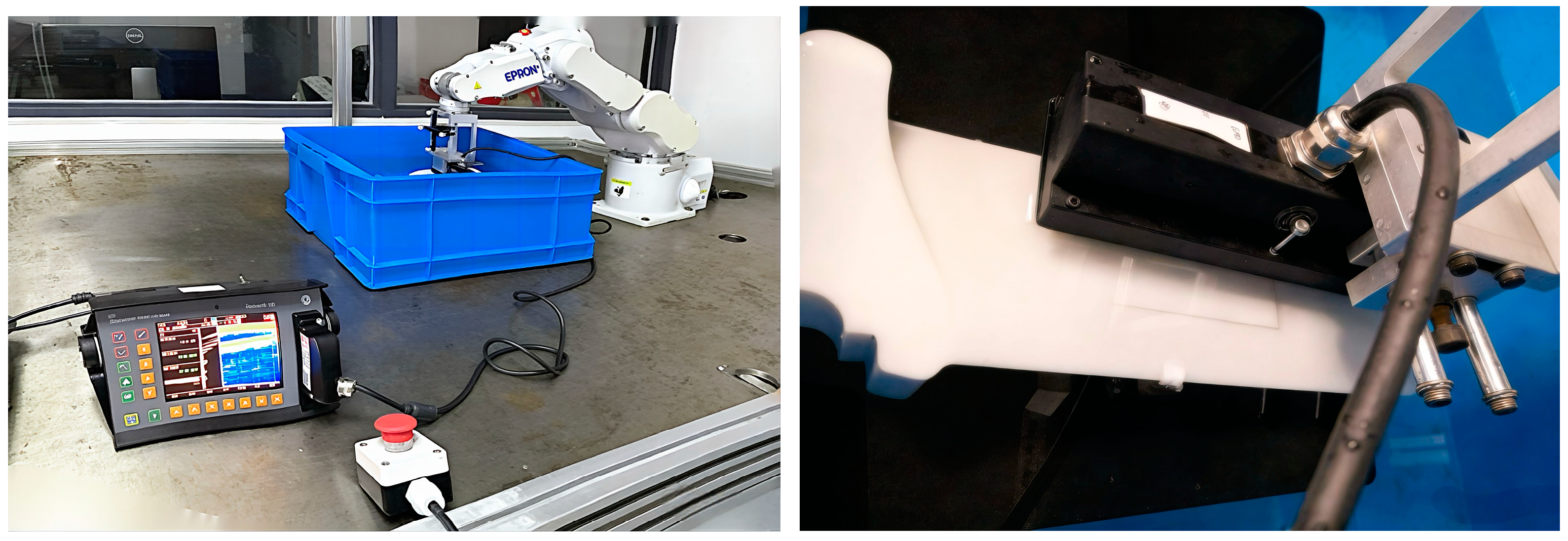
The experiment used an Epson C3 six-axis robot to carry an ultrasonic probe for scanning. The water immersion method was employed to conduct ultrasonic flaw detection on the engine blade model, as shown in Figure 17. The end of the robot hand carried the ultrasonic probe and was submerged in the water to perform vertical incidence ultrasonic flaw detection on the aircraft engine blades.

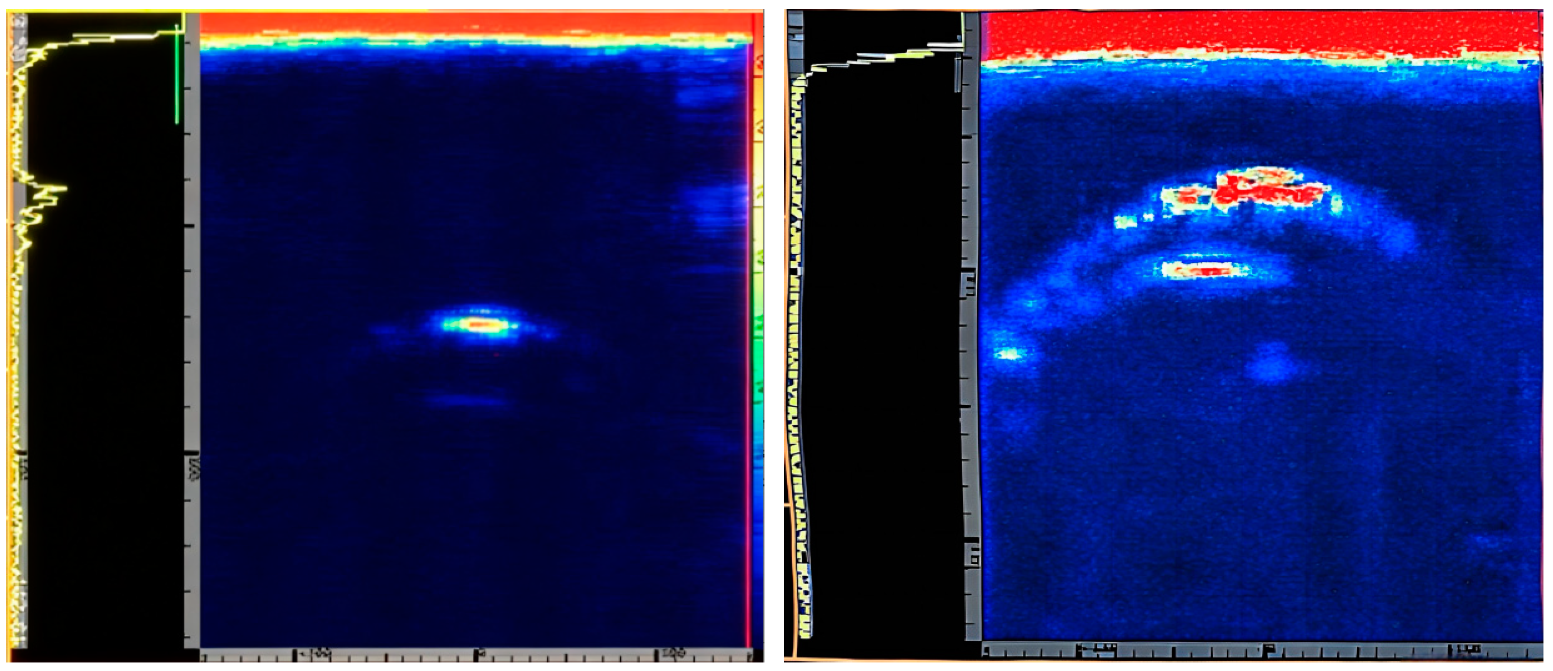
At the scanning position, an ultrasonic image is obtained based on the coordinate variation in the width direction of the engine blade. By moving relatively by −10° to +10°, an ultrasonic image can be obtained in Figure 18. It can be observed that when the curve deviates by 1°, the average gray value image feature is reduced by 1.71%; when it deviates by 2°, the average gray value image feature is reduced by 7.81%; and when it deviates by 5°, the average reduction is 16.77%.

5. Conclusions

This paper investigates trajectory planning for six-axis robotic-arm-aided nondestructive testing (NDT). Surface paths are specified through gesture input, enabling the automatic generation of trajectories for applications such as ultrasonic nondestructive testing and surface welding. By employing a Leap Motion-based gesture recognition device, the programming complexity associated with sophisticated robot motion trajectories is significantly reduced, and both point-to-point and continuous trajectories are optimized. The proposed approach not only realizes gesture-based robot trajectory control but also mitigates gesture-induced errors during trajectory processing, adapts to varying scanning speeds corresponding to different surface curvatures, and smooths trajectories to effectively reduce dynamic impact forces.

(1) Kinematic modeling and gesture-based trajectory generation. Taking the Epson C3 robot as a representative example, a six-degree-of-freedom kinematic model was established. An engine blade CAD model was imported into the robot workspace, and a Leap Motion gesture recognition device was used to acquire the initial gesture trajectory along the target surface. The CAD model, gesture trajectory, and human–robot coordinate spaces were unified within the robot coordinate system to obtain the robot pose trajectory corresponding to the gesture path. Based on a PSO hybrid algorithm, inverse kinematic solutions in the robot joint space were derived. Interpolation fitting and time–impact optimization were performed on the joint angles corresponding to each trajectory pose point, preventing excessive joint velocities caused by normal-direction extension in regions of high surface curvature. The time intervals between successive trajectory points were subsequently replanned.

(2) Continuous trajectory optimization under acceleration constraints. In continuous trajectory planning, the spacing between adjacent trajectory points is relatively small, resulting in limited effectiveness of acceleration control. Therefore, trajectory optimization was conducted under explicit acceleration constraints. Cubic spline interpolation, circular arc interpolation, and non-uniform rational B-spline (NURBS) interpolation were applied to interpolate and optimize the joint-space trajectory point sequence. The results indicate that cubic spline interpolation achieved the shortest execution time of 8.9970 s, while the maximum and minimum angular velocities obtained using NURBS interpolation were 1.0767 rad/s.

(3) Point-to-point trajectory optimization using 5-5-5 polynomial interpolation. For point-to-point trajectory planning involving four trajectory points, a 5-5-5 polynomial interpolation scheme was adopted. Intelligent optimization algorithms were employed to optimize three time intervals under constraints on velocity, acceleration, and jerk, yielding the corresponding fifth-degree polynomial coefficients. The optimized trajectory achieved a total execution time of 4.0894 s, with a maximum angular velocity of 1.3707 rad/s, a maximum angular acceleration of 4.8531 rad/s², and a maximum angular jerk of 14.7562 rad/s³. The resulting trajectory is smooth, with a short execution time and favorable dynamic performance.

6. Prospect

This research introduced jitter/acceleration constraints to ensure the performance of the trajectory movement and found the quantification of impact and tracking accuracy is highly inspiring for verifying the laws that affect the quality of ultrasonic detection signals. Furthermore, by comparing peak acceleration, cumulative acceleration, and the root mean square error of posture with the normal values from CAD, as well as evaluating the deviation of the end effector against the reference value, we found the correlations and scientific laws between the quality of ultrasonic detection signals and these parameters. This approach will also enable decreasing the noise impact of the Leap Motion device, which will be further mitigated, overcoming real-time limitations and the resolution of the coupling and force control issues associated with UT.

References

1. Gupta, M.; Khan, M.A.; Butola, R.; Singari, R.M. Advances in applications of Non-Destructive Testing (NDT): A review. Adv. Mater. Process. Technol. 2022, 8, 2286–2307. [Google Scholar] [CrossRef] [Scilit]
2. Abdollahi-Mamoudan, F.; Ibarra-Castanedo, C.; Maldague, X.P.V. Non-destructive testing and evaluation of hybrid and advanced structures: A comprehensive review of methods, applications, and emerging trends. Sensors 2025, 25, 3635. [Google Scholar] [CrossRef] [Scilit]
3. Cheng, L.; Gao, H.B.; Sun, W.F.; Chen, C.; Xu, X. An integrated method for predictive state assessment and path planning for inspection robots in island-based unmanned substations. Eksploat. Niezawodn. Maint. Reliab. 2025, 27, 203994. [Google Scholar] [CrossRef] [Scilit]
4. Chen, C.; Chen, L.; Zhou, X. Design and implementation of industrial robot teaching system based on natural gesture interaction. Manuf. Autom. 2018, 40, 21–25. [Google Scholar]
5. Gao, L.F.; Wang, W.D.; Ke, D.Y. Energy Optimization for Autonomous Mobile Robot Path Planning Based on Deep Reinforcement Learning. Comput. Mater. Contin. 2025, 86, 1–15. [Google Scholar] [CrossRef] [Scilit]
6. Lv, Y.H.; Yao, R.; Yan, Y.L. The Optimal Trajectory Planning of Industrial Robot Based on Gesture Recognition. Modul. Mach. Tool Autom. Manuf. Tech. 2019, 9, 50–54. [Google Scholar]
7. Liu, Y.; Xiao, F.; Tong, X.; Tao, B.; Xu, M.; Jiang, G.; Chen, B.; Cao, Y.; Sun, N. Manipulator trajectory planning based on work subspace division. Concurr. Comput. Pract. Exp. 2022, 34, e6710. [Google Scholar] [CrossRef] [Scilit]
8. Yu, X.; Dong, M.; Yin, W. Time-optimal trajectory planning of manipulator with simultaneously searching the optimal path. Comput. Commun. 2022, 181, 446–453. [Google Scholar] [CrossRef] [Scilit]
9. Zhang, T.; Zhang, M.; Zou, Y. Time-optimal and smooth trajectory planning for robot manipulators. Int. J. Control. Autom. Syst. 2021, 19, 521–531. [Google Scholar] [CrossRef] [Scilit]
10. Jin, R.; Rocco, P.; Geng, Y. Cartesian trajectory planning of space robots using a multi-objective optimization. Aerosp. Sci. Technol. 2021, 108, 106360. [Google Scholar] [CrossRef] [Scilit]
11. Fu, R.; Ju, H. Time optimal trajectory planning algorithm for robotic arms based on AGA. Comput. Appl. Res. 2011, 28, 3275–3278. [Google Scholar]
12. Gasparetto, A.; Lanzutti, A.; Vidoni, R.; Zanotto, V. Experimental validation and comparative analysis of optimal time-jerk algorithms for trajectory1 planning. Robot. Comput. Integr. Manuf. 2012, 28, 164–181. [Google Scholar] [CrossRef] [Scilit]
13. Yang, J.; Jiang, W.; Lin, Y. An Optimal Trajectory Planning Algorithm for Industrial Robot Impact. Sci. Technol. Eng. 2014, 14, 64–69. [Google Scholar]
14. Yu, Y.; Lin, M.; Lin, Y. Optimal trajectory planning of industrial robots based on hybrid genetic algorithm. Comput. Eng. Des. 2012, 33, 1574–1580. [Google Scholar]
15. Lin, H.I. A Fast and Unified Method to Find a Minimum-Jerk Robot Joint Trajectory Using Particle Swarm Optimization. J. Intell. Robot. Syst. 2014, 75, 379–392. [Google Scholar] [CrossRef] [Scilit]
16. You, T.; Zhang, W.; Ge, L. Research on path planning for welding robots based on GA-PSO algorithm. J. Liaoning Univ. Petrochem. Technol. 2018, 38, 85–89. [Google Scholar]
17. Akiyoshi, T.; Sumioka, H.; Nakanishi, J.; Kato, H.; Shiomi, M. Modeling and implementation of intra-hug gestures during dialogue for a huggable robot. IEEE Robot. Autom. Lett. 2025, 10, 3498697. [Google Scholar] [CrossRef] [Scilit]
18. Madridano, A.; Al-Kaff, A.; Martín, D.; De La Escalera, A. Trajectory planning for multi-robot systems: Methods and applications. Expert Syst. Appl. 2021, 173, 114660. [Google Scholar] [CrossRef] [Scilit]
19. Dai, Y.; Xiang, C.; Zhang, Y.; Jiang, Y.; Qu, W.; Zhang, Q. A Review of spatial robotic arm trajectory planning. Aerospace 2022, 9, 361. [Google Scholar] [CrossRef] [Scilit]
20. Song, Q.; Li, S.; Bai, Q.; Yang, J.; Zhang, A.; Zhang, X.; Zhe, L. Trajectory planning of robot manipulator based on RBF neural network. Entropy 2021, 23, 1207. [Google Scholar] [CrossRef] [Scilit] [PubMed]
21. Roda-Sanchez, L.; Olivares, T.; Garrido-Hidalgo, C.; de la Vara, J.L.; Fernandez-Caballero, A. Human-robot interaction in Industry 4.0 based on an Internet of Things real-time gesture control system. Integr. Comput. Aided Eng. 2021, 28, 159–175. [Google Scholar] [CrossRef] [Scilit]
22. Salman, A.E.; Roman, M.R. Augmented reality-assisted gesture-based teleoperated system for robot motion planning. Ind. Robot. Int. J. Robot. Res. Appl. 2023, 50, 765–780. [Google Scholar] [CrossRef] [Scilit]
23. Mohamed, N.; Mustafa, M.B.; Jomhari, N. A review of the hand gesture recognition system: Current progress and future directions. IEEE Access 2021, 9, 157422–157436. [Google Scholar] [CrossRef] [Scilit]
24. Shen, J.; Chen, L. Application of human posture recognition and classification in performing arts education. IEEE Access 2024, 12, 125906–125919. [Google Scholar] [CrossRef] [Scilit]
25. Rahman, M.M.; Uzzaman, A.; Khatun, F.; Aktaruzzaman, M.; Siddique, N. A comparative study of advanced technologies and methods in hand gesture analysis and recognition systems. Expert Syst. Appl. 2025, 266, 125929. [Google Scholar]
26. Lozer, F.; Scalera, L.; Boscariol, P.; Gasparetto, A. Planning optimal minimum-jerk trajectories for redundant robots. Robot. Auton. Syst. 2025, 192, 105049. [Google Scholar] [CrossRef] [Scilit]
27. Xiao, Z.Y.; Sun, D.F.; Zhu, D.L.; Wang, Y.; Yan, Y.; Wu, H. Time-torque coordinated optimization for trajectory planning of industrial robots. Robot. Comput. Integr. Manuf. 2026, 99, 103199. [Google Scholar] [CrossRef] [Scilit]
28. Hazem, Z.B.; Saidi, F.; Guler, N.; Altaif, A.H. A hybrid reinforcement learning framework combining td3 and PID control for robust trajectory tracking of a 5-dof robotic arm. Automation 2025, 6, 56. [Google Scholar] [CrossRef] [Scilit]
Figure 1. Gesture data modeling and collection. A, B, C, D are the four endpoints of the curve surface in the Cartesian coordinate system. D is the calculate reference for coordinate transformation.
Coatings 16 00332 g001
Figure 2. Initial gesture coordinate trajectory. The red circles represent the gesture sampling points; the blue lines represent the gesture trajectories.
Coatings 16 00332 g002
Figure 3. Filtering processing. (a) Median filtering processing; (b) mean filtering processing. The red line represents the original trajectory; the blue * represents the filtered trajectory.
Coatings 16 00332 g003
Figure 4. Coordinates of robot space orbital points.
Coatings 16 00332 g004
Figure 5. Attitude simulation of robot motion process.
Coatings 16 00332 g005
Figure 6. Tangent double circular arc splines.
Coatings 16 00332 g006
Figure 7. Cubic spline interpolation for joint-space trajectory with continuous trajectory optimization. Blue * represents the control vertex.
Coatings 16 00332 g007
Figure 8. Single-arc interpolation for joint-space trajectory with continuous trajectory optimization. Blue * represents the control vertex.
Coatings 16 00332 g008
Figure 9. Three-dimensional B-spline interpolation for joint-space trajectory with continuous trajectory optimization. Blue * represents the control vertex.
Coatings 16 00332 g009
Figure 10. Cartesian space coordinate trajectory and robot trajectory simulation. (a) NURBS interpolation positive solution cartesian space trajectory. (b) MATLAB robot toolbox simulation.
Coatings 16 00332 g010
Figure 11. Find the inverse kinematics solution for the four points and optimize the four trajectory points.
Coatings 16 00332 g011
Figure 12. The optimal time interval under the constraint of four-point trajectory of six joints.
Coatings 16 00332 g012
Figure 13. Optimal time for six-axis curve of four trajectory points under constraints. (a) The optimal curve for the angle, velocity, acceleration, and jerk of the first three axes; (b) the optimal curve for the angle, velocity, acceleration, and jerk of the rear three axes.
Coatings 16 00332 g013
Figure 14. Manipulator end trajectory. (a) Original gesture trajectory and optimized trajectory; (b) path points in simulation. The blue line represents the original trajectory; the red line represents the optimized trajectory.
Coatings 16 00332 g014
Figure 15. Leap Motion device.
Coatings 16 00332 g015
Figure 16. Experimental data.
Coatings 16 00332 g016
Figure 17. Ultrasonic scanning equipment and attitude.
Coatings 16 00332 g017
Figure 18. Ultrasonic images before and after planning (engine blade width direction). The red area represents the outline of the engine blade surface.
Coatings 16 00332 g018