Non-Monotonic Effect of Substrate Inhibition in Conjunction with Diffusion Limitation on the Response of Amperometric Biosensors

Abstract

The non-monotonic behavior of amperometric enzyme-based biosensors under uncompetitive and noncompetitive (mixed) substrate inhibition is investigated computationally using a two-compartment model consisting of an enzyme layer and an outer diffusion layer. The model is based on a system of reaction–diffusion equations that includes a nonlinear term associated with non-Michaelis–Menten kinetics of the enzymatic reaction and accounts for the partitioning between layers. In addition to the known effect of substrate inhibition, where the maximum biosensor current differs from the steady-state output, it has been determined that external diffusion limitations can also cause the appearance of a local minimum in the current. At substrate concentrations greater than both the Michaelis–Menten constant and the uncompetitive substrate inhibition constant, and in the presence of external diffusion limitation, the transient response of the biosensor, after immersion in the substrate solution, may follow a five-phase pattern depending on the model parameter values: it starts from zero, reaches a global or local maximum, decreases to a local minimum, increases again, and finally decreases to a steady intermediate value. The biosensor performance is analyzed numerically using the finite difference method.

1. Introduction

Enzyme-based amperometric biosensors were the first type of biosensors developed and remain the most popular due to their simplicity, ease of production, and low cost [1,2,3]. They measure changes in the output current at the working electrode caused by the direct oxidation or reduction of biochemical reaction products. The amperometric response is typically proportional to the analyte (substrate) concentration in a buffer solution [2,4,5,6]. These devices have found widespread applications in clinical, environmental, industrial, toxin detection, and other fields [3,7,8,9,10,11].

Most biosensors operate according to the Michaelis–Menten kinetics scheme,

$$\mathrm{E}+\mathrm{S}\underset{k_{-1}}{\overset{k_1}{\rightleftharpoons }}\mathrm{ES}\stackrel{k_2}{\to }\mathrm{E}+\mathrm{P},$$

(1)

where E is an enzyme, S is a substrate, $\mathrm{ES}$ is an enzyme–substrate complex, $\mathrm{P}$ is a reaction product, and $k_1$, $k_{-1}$ and $k_2$ are the rate constants [2,4,5,7].

Often, the kinetics of the enzyme-based biosensors are much more complicated than in the simplest scheme (1). Different substances may act as inhibitors and cause a reduction in the rate of an enzyme-catalyzed reaction [6,8,12,13]. The substrate in many enzyme-catalyzed reactions behaves as an inhibitor. In addition to the scheme (1), the interaction of the enzyme–substrate complex (ES) with other substrate molecules (S), resulting in the formation of a non-active inhibitory complex (ESS), can give rise to one of the simplest non-Michaelis–Menten mechanisms of enzyme action—uncompetitive substrate inhibition:

$$\mathrm{ES}+\mathrm{S}\underset{k_{-3}}{\overset{k_3}{\rightleftharpoons }}\mathrm{ESS},$$

(2)

where $k_3$ and $k_{-3}$ are the rate constants [2,3,6,8,14].

A second substrate molecule can also bind to a regulatory site on the free enzyme (E), leading to the formation of an inactive or less active complex (ESI). This phenomenon is referred to as competitive substrate inhibition:

$$\mathrm{E}+\mathrm{S}\underset{k_{-4}}{\overset{k_4}{\rightleftharpoons }}\mathrm{ESI},$$

(3)

where $k_4$ and $k_{-4}$ are the rate constants [2,3,6,8,15,16].

In more complex systems involving noncompetitive (mixed) substrate inhibition, excess substrate can bind to both the free enzyme (E) and the enzyme–substrate complex (ES), resulting in the formation of inactive complexes in both pathways [12,14,17,18].

Understanding the kinetic properties of biosensors is crucial for their design and optimization [19,20,21]. Mathematical modeling has proven to be a useful tool to study the effect of enzyme inhibition [10,11,15,17,22,23,24,25]. Various approaches have been applied for the biosensor modeling [26,27,28,29,30]. Actual biosensors with substrate inhibition have already been modeled at various, often steady-state, conditions [16,18,31,32,33,34]. The amperometric biosensors utilizing the enzyme with the substrate inhibition have also been modeled at the external diffusion limitation and the steady-state [10,22] as well as the transition conditions [30,35,36].

In particular, Kulys showed that a multi-steady-state response can be generated at the electrode surface under external diffusion limitations when the substrate concentration is much greater than the Michaelis–Menten constant, assuming an extremely thin enzyme layer [22]. However, to the best of our knowledge, only non-monotonic transient responses featuring a maximum followed by a final steady-state current have been simulated [24,31,35,36,37,38]. In such cases, the response typically follows a three-phase pattern: starting from zero, reaching a maximum, and finally decreasing to a steady value.

When modeling practical biosensors, multi-layer models are usually required to achieve sufficient accuracy of the model [31,39,40]. Nevertheless, even mono-layer models that neglect external mass transport by diffusion have still been used in various applications in recent years due to the model’s simplicity [14,15,24,38,41,42,43,44,45]. However, external mass transport by diffusion significantly influences the dynamics of the catalytic processes in enzyme-loaded systems in general and biosensor response and sensitivity in particular [9,46,47,48,49,50]. Fortunately, mass transport through several outer diffusion layers can be rather effectively approximated by a single diffusion layer with effective diffusion coefficients [51,52,53]. As a result, two-compartment models have been widely used in biosensor modeling [10,39,54,55,56,57,58,59].

The aim of this work was to investigate in detail the influence of substrate inhibition, in conjunction with internal and external diffusion limitations, on the transient response of enzyme-based amperometric biosensors under uncompetitive, competitive, and noncompetitive (mixed) substrate inhibition. This study focuses on the conditions under which the transient response of the biosensor, after being immersed in a substrate solution, exhibits a complex, multi-phase pattern, characterized by the appearance of a local minimum, a local maximum, or even both.

Under transient conditions, a biosensor is mathematically modeled using a two-compartment model comprising a mono-enzyme layer, where both the enzymatic reaction and mass transport by diffusion occur, and a diffusion-limiting region, where only mass transport by diffusion takes place. The model is based on a system of reaction–diffusion equations that includes a nonlinear term associated with non-Michaelis–Menten kinetics of the enzymatic reaction and accounts for partitioning between layers. The performance of the treated system is analyzed numerically using the finite difference technique [60,61], and the simulation results are compared with previous studies on biosensors under substrate inhibition [22,24,31,35,36].

2. Mathematical and Computational Modeling

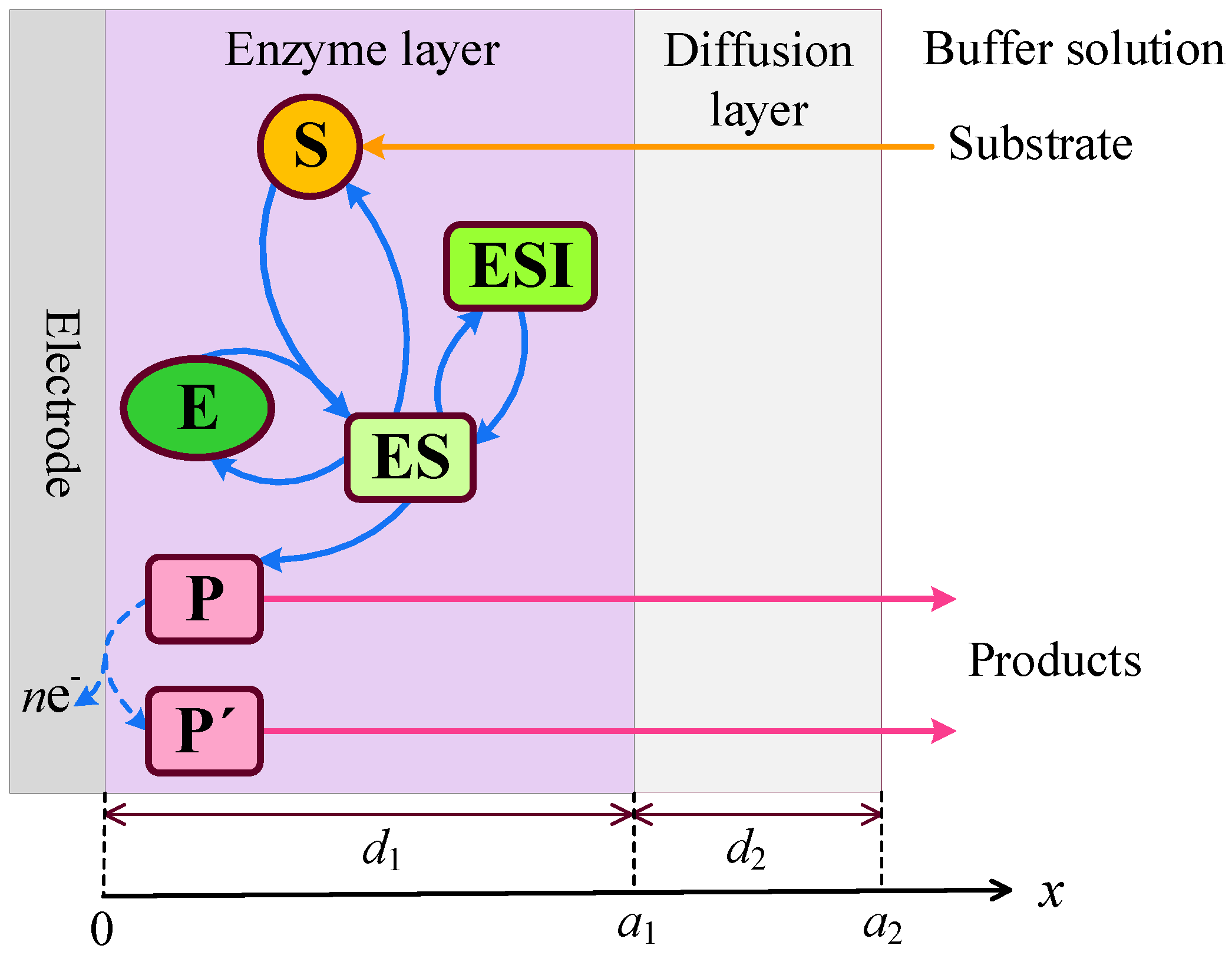
2.1. Biosensor Principal Structure

An amperometric biosensor consists of an electrode coated with a relatively thin enzyme layer, also referred to as the enzyme membrane [2,4,6,7,9]. The model describes three distinct regions: the enzyme layer, where both enzymatic reactions and diffusion-driven mass transport occur; a diffusion-limiting region, where only diffusion-based mass transport takes place; and a convective region, where the analyte concentration remains constant [35,36]. A schematic representation of the biosensor model is shown in Figure 1, where $d_1$ and $d_2$ denote the thicknesses of the enzyme layer and the outer diffusion layer, respectively.

In the enzyme layer, we account for the enzyme-catalyzed reactions described by Equations (1)–(3). At the electrode surface, the electro-active product $\mathrm{P}$ is converted into a non-interfering species ${\mathrm{P}}^{\prime }$, releasing electrons in the process,

$$\mathrm{P}\to {\mathrm{P}}^{\prime }\pm n{\mathrm{e}}^{-}$$

(4)

where n is the number of electrons transferred in the reaction.

Some reactions in the network (1)–(4) occur very rapidly, while others proceed much more slowly [2,4,6,7,9]. This wide disparity in reaction timescales complicates both the simulation of the network dynamics and the understanding of its fundamental behavior. To address these challenges, the quasi-steady-state approximation (QSSA) is commonly employed [62,63].

Under the assumption of the QSSA, the concentrations of the enzyme (E) and the intermediate complexes (ES, ESS, and ESI) remain constant over time. As a result, the rate of the biochemical reaction is described by the following equation, which does not follow Michaelis–Menten kinetics:

$$\begin{array}{cc}\hfill & V\left(S\right)={\displaystyle \frac{V_{max}S}{K_M(1+S/K_I^{\prime })+S(1+S/K_I)}},\hfill \\ \hfill V_{max}=k_2{E}_0,& K_M=(k_{-1}+k_2)/k_1,K_I=k_{-3}/k_3,K_I^{\prime }=k_{-4}/k_4,\hfill \end{array}$$

(5)

where S is the substrate concentration, $V_{max}$ is the maximal enzymatic rate, $E_0$ is the total enzyme concentration, $K_M$ is the Michaelis constant, and $K_I$ and $K_I^{\prime }$ are the inhibition (dissociation) constants [4,14,16,17,64,65].

At very low substrate concentrations, where $S\ll K_M$, $S\ll K_I$ and $S\ll K_I^{\prime }$, the nonlinear reaction rate given in (5) simplifies to the first-order reaction rate $V_{max}S/K_M$. At high substrate concentrations such that $S\gg K_M$ but still $S\ll K_I$ and $S\ll K_I^{\prime }$, the rate becomes independent of the substrate concentration, exhibiting zero-order kinetics. The influence of inhibition on the overall biochemical process decreases as the inhibition constants $K_I$ and $K_I^{\prime }$ increase, and the kinetics gradually approach the standard Michaelis–Menten kinetics form as $K_I\to \infty$ and $K_I^{\prime }\to \infty$.

In the case of uncompetitive substrate inhibition ($K_I^{\prime }\to \infty$), where only two enzymatic reactions (1) and (2) occur, the reaction rate reduces to:

$$V\left(S\right)={\displaystyle \frac{V_{max}S}{K_M+S+S^2/K_I}},K_I^{\prime }\to \infty .$$

(6)

When $S>K_I$, the inhibitory term $S^2/K_I$ in the denominator becomes significant, and the reaction rate begins to decline despite the increasing substrate concentration [4,64].

When the biosensor operates under competitive substrate inhibition (with $K_I\to \infty$), the reaction rate can be rewritten in Michaelis–Menten form,

$$\begin{array}{cc}\hfill & V\left(S\right)={\displaystyle \frac{V_{max}S}{K_M(1+S/K_I^{\prime })+S}}={\displaystyle \frac{V_{max}^{\mathrm{eff}}S}{K_M^{\mathrm{eff}}+S}},K_I\to \infty ,\hfill \\ \hfill & V_{max}^{\mathrm{eff}}={\displaystyle \frac{V_{max}}{1+K_M/K_I^{\prime }}},K_M^{\mathrm{eff}}={\displaystyle \frac{K_M}{1+K_M/K_I^{\prime }}}.\hfill \end{array}$$

(7)

Here, $V_{max}^{\mathrm{eff}}$ and $K_M^{\mathrm{eff}}$ represent the apparent or effective kinetic parameters under competitive substrate inhibition. They correspond to the effective maximal enzymatic rate and Michaelis constant, respectively. Thus, the behavior of enzyme-based biosensors under competitive substrate inhibition can be described using modified kinetic expressions that extend beyond the classical Michaelis–Menten model.

The biochemical reactions occurring in practical biosensors are influenced by various important biosensor-related factors such as pH, enzyme concentration, cofactor availability, temperature, enzyme degradation over time, and others [2,4,5,7,12,15,25]. Under certain conditions, these factors are commonly incorporated into the Michaelis–Menten parameters and inhibition constants. Although they are not part of the original Michaelis–Menten derivation, they are often embedded empirically through experimental observations. In biosensor modeling, these adjusted parameters are typically referred to as the “apparent” or “effective” $V_{max}^{\mathrm{eff}}$ and $K_M^{\mathrm{eff}}$ [8,9,12,14,30,58].

This work focuses on the impact of uncompetitive and noncompetitive substrate inhibition and is restricted to substrate concentrations greater than at least one of the inhibition constants, $K_I$ or $K_I^{\prime }$.

In the two-compartment (or two-layer) model, the diffusion layer is commonly considered to be the Nernst diffusion layer [9,60,66]. However, if the external Nernst diffusion layer is neglected, the diffusion layer can instead be modeled as a semi-permeable (diffusion-limiting) membrane [30,39,48,60,67]. It is important to note, though, that a Nernst layer with zero thickness cannot be realized in practice [68].

Mathematical models of biosensors sometimes account for both the outer membrane and the Nernst diffusion layer [31,52,53,69]. However, the mass transport across multiple diffusion layers can often be effectively approximated by a single layer with adjusted diffusion coefficients, allowing a complex multi-compartment model to be simplified into a two-compartment one [51,52,53]. As a result, the effects examined in this study are also applicable to amperometric biosensors modeled with several diffusion layers, including both the outer membrane and the Nernst layer.

2.2. Mathematical Model

Assuming symmetrical geometry of the electrode, enzymatic, and diffusion layers, as well as uniform distribution of the immobilized enzyme within the enzyme membrane, leads to a two-compartment mathematical model defined in a one-dimensional spatial domain. This model is expressed as an initial boundary value problem that captures the dynamics of substrate and product concentrations [8,30,39,70].

2.2.1. Governing Equations

The changes in the concentrations of the substrate S and product P within the enzyme layer over time are governed by a system of reaction–diffusion equations ($t>0$),

$$\begin{array}{cc}\hfill {\displaystyle \frac{\partial S_1}{\partial t}}& =D_{S_1}{\displaystyle \frac{{\partial }^2{S}_1}{\partial x^2}}-{\displaystyle \frac{V_{max}{S}_1}{K_M(1+S_1/K_I^{\prime })+S_1(1+S_1/K_I)}},\hfill \\ \hfill {\displaystyle \frac{\partial P_1}{\partial t}}& =D_{P_1}{\displaystyle \frac{{\partial }^2{P}_1}{\partial x^2}}+{\displaystyle \frac{V_{max}{S}_1}{K_M(1+S_1/K_I^{\prime })+S_1(1+S_1/K_I)}},x\in (0,a_1),\hfill \end{array}$$

(8)

where $S_1(x,t)$ and $P_1(x,t)$ are the concentrations of the substrate and the product in the enzyme layer, $D_{S_1}$ and $D_{P_1}$ are the diffusion coefficients, $d_1=a_1$ is the thickness of the enzyme layer, and $V\left(S_1\right)$ is the reaction rate, as defined in (5) [8,39,64].

In the diffusion layer, both compounds are transported solely by diffusion ($t>0$),

$$\begin{array}{cc}\hfill {\displaystyle \frac{\partial S_2}{\partial t}}& =D_{S_2}{\displaystyle \frac{{\partial }^2{S}_2}{\partial x^2}},\hfill \\ \hfill {\displaystyle \frac{\partial P_2}{\partial t}}& =D_{P_2}{\displaystyle \frac{{\partial }^2{P}_2}{\partial x^2}},x\in (a_1, a_2),\hfill \end{array}$$

(9)

where $S_2(x,t)$ and $P_2(x,t)$ are the concentrations of the substrate and the reaction product, $D_{S_2}$, $D_{P_2}$ are the diffusion coefficients, $a_2=a_1+d_2$, and $d_2$ is the thickness of the diffusion layer [8,30,39].

2.2.2. Boundary Conditions

During biosensor operation, the concentrations of the substrate and product remain constant in the bulk solution ($t>0$),

$$S_2(a_2,t)=S_0,P_2(a_2,t)=0,$$

(10)

where $S_0$ is the concentration of the substrate in the bulk.

At the boundary between adjacent layers, the fluxes of the substrate and product are assumed to be equal; that is, the outgoing flux from one layer equals the incoming flux to the next. However, the concentrations on either side of the interface differ and are related by the formal partition coefficients ${\theta }_S$ for the substrate and ${\theta }_P$ for the product ($t>0$) [69,70,71,72,73],

$$\begin{array}{cc}\hfill & D_{S_1}{\displaystyle \frac{\partial S_1}{\partial x}}{|}_{x=a_1}=D_{S_2}{\displaystyle \frac{\partial S_2}{\partial x}}{|}_{x=a_1},S_1(a_1,t)={\theta }_S{S}_2(a_1,t),\hfill \\ \hfill & D_{P_1}{\displaystyle \frac{\partial P_1}{\partial x}}{|}_{x=a_1}=D_{P_2}{\displaystyle \frac{\partial P_2}{\partial x}}{|}_{x=a_1},P_1(a_1,t)={\theta }_P{P}_2(a_1,t).\hfill \end{array}$$

(11)

The partition coefficients are generally different for different species [72,74], but they are often assumed to be identical [10,53,58,69,71].

Due to the electrochemical reaction (4), the concentration of the reaction product decreases at the electrode surface. The substrate is considered electrically inactive, and no concentration flux is assumed for it ($t>0$) [8,39,75],

$$P_1(0,t)=0,D_{S_1}{\displaystyle \frac{\partial S_1}{\partial x}}{|}_{x=0}=0,t>0.$$

(12)

2.2.3. Initial Conditions

Two different initial conditions corresponding to two modes of biosensor operation are considered.

In the first mode, the biosensor is assumed to be permanently immersed in a buffer solution, and its operation begins when the analyte (substrate) is introduced at $t=0$ into the buffer solution,

$$\begin{array}{cc}\hfill & S_1(x,0)=0,P_1(x,0)=0,x\in [0,a_1],\hfill \\ \hfill & S_2(x,0)=0,P_2(x,0)=0,x\in [a_1,a_2),\hfill \\ \hfill & S_2(a_2,0)=S_0,P_2(a_2,0)=0.\hfill \end{array}$$

(13)

This setup simulates injection analysis (IA) or real-time monitoring, where the analyte arrival initiates the biosensor transient response [8,9,10,15,31,56,76].

The second type of operation is common in batch analysis (BA), when the biosensor is directly immersed in a buffer solution containing the analyte [8,9,25,58,77]. The biosensor operation starts responding to the analyte from the moment of immersion. In this case, the initial conditions (13) have to be replaced with the following:

$$\begin{array}{cc}\hfill & S_1(x,0)=0,P_1(x,0)=0,x\in [0,a_1),\hfill \\ \hfill & S_1(a_1,0)={\theta }_S{S}_0,P_1(a_1,0)=0,\hfill \\ \hfill & S_2(x,0)=S_0,P_2(x,0)=0,x\in [a_1,a_2].\hfill \end{array}$$

(14)

Let us notice that both initial conditions, (13) and (14), result in the same steady-state solution for the problem (8)–(12). Only the transient solution is affected by the initial conditions [8,30,39,60].

The two-compartment model defined by Equations (8)–(14) converges to the corresponding one-compartment model as $a_2\to a_1$ ($d_2\to 0$) [15,38,41,42,44,45].

2.3. Biosensor Response

The amperometric electrode detects the faradaic current, whether anodic or cathodic in nature [2,8,64]. The current density $I\left(t\right)$ at time t can be explicitly derived using Faraday’s and Fick’s laws,

$$I\left(t\right)=nF{D}_{P_1}{\displaystyle \frac{\partial P_1}{\partial x}}{|}_{x=0},$$

(15)

where n is the number of electrons involved in a charge transfer at the electrode surface, and F is the Faraday constant [8,39,75].

As $t\to \infty$, the system (8)–(12) approaches a steady state [8,39,64],

$$I_{\mathrm{ss}}=\underset{t\to \infty }{lim}I\left(t\right),$$

(16)

where $I_{\mathrm{ss}}$ is the density of the steady-state output current.

Since the transient current in the case of the enzyme inhibition can be a non-monotonic function of time, the maximal current has also been used as a characteristic for this kind of biosensor [24,31,35,36,37,38]. Aiming to determine conditions under which biosensor response follows a multi-phase pattern, the number $N_{\mathrm{ext}}$ of extrema in transient output current $I\left(t\right)$ was studied. A local or global maximum of output current $I\left(t\right)$ occurs at time $t=t_e$ if $I\left(t_e\right)\ge I\left(t\right)$ for all t near $t_e$, while a local minimum occurs at that time $t=t_e$ if $I\left(t_e\right)\le I\left(t\right)$ for all t near $t_e$. $N_{\mathrm{ext}}$ is considered as the total count of maxima and minima that the function $I\left(t\right)$ has at $t>0$,

$$N_{\mathrm{ext}}=\left|\left\{t>0|{\displaystyle \frac{\mathrm{d}I\left(t\right)}{\mathrm{d}t}}=0\mathrm{and}{\displaystyle \frac{{\mathrm{d}}^{2}I\left(t\right)}{\mathrm{d}{t}^2}}\ne 0\right\}\right|,$$

(17)

where $\left|·\right|$ denotes the set cardinality and the condition for defining the set.

In the specific case of a monotonic output current, $I\left(t\right)$, $N_{\mathrm{ext}}$ = 0. In the case of a three-phase pattern, when the output current starts from zero, reaches a maximum, and then decreases to a steady value, $N_{\mathrm{ext}}$ = 1. $N_{\mathrm{ext}}$ = 2 when the biosensor response approaches a four-phase pattern, exhibiting a local minimum in addition to the maximum.

2.4. Dimensionless Model Parameters

To identify the key governing parameters of the mathematical model, a dimensionless form is typically derived [66,69]. The two-compartment model (8)–(12) was transformed into a dimensionless form by rescaling time and space [30,36,48]. This process yielded the following dimensionless governing parameters:

$$\begin{array}{cc}\hfill x^{*}={\displaystyle \frac{x}{a_1}},t^{*}& ={\displaystyle \frac{D_{S_1}t}{a_1^2}},S_0^{*}={\displaystyle \frac{S_0}{K_M}},K_I^{*}={\displaystyle \frac{K_I}{K_M}},K_I^{\prime }*={\displaystyle \frac{K_I^{\prime }}{K_M}},\hfill \\ \hfill S_i^{*}& ={\displaystyle \frac{S_i}{K_M}},P_i^{*}={\displaystyle \frac{P_i}{K_M}},i=1,2,\hfill \\ \hfill {\sigma }^2={\displaystyle \frac{V_{max}{d}_1^2}{K_M{D}_{S_1}}}& ,{\beta }_S={\displaystyle \frac{D_{S_2}{d}_1}{{\theta }_S{D}_{S_1}{d}_2}},{\beta }_P={\displaystyle \frac{D_{P_2}{d}_1}{{\theta }_P{D}_{P_1}{d}_2}},\hfill \\ \hfill I^{*}\left(t^{*}\right)& ={\displaystyle \frac{I\left(t\right)d_1}{n_{e}F{D}_{S_1}{K}_M}},I_{ss}^{*}=\underset{t^{*}\to \infty }{lim}{I}^{*}\left(t^{*}\right),\hfill \end{array}$$

(18)

where ${\sigma }^2$ is the dimensionless Damköhler number (the Thiele modulus squared) or the diffusion module, and ${\beta }_S$ and ${\beta }_P$ are the Biot numbers for the substrate and product, respectively [39,75,78,79]. Equations (8)–(12) in dimensionless form are presented in the Appendix A. All of the dimensional and dimensionless model parameters are listed in

Table A1. Dimensional and dimensionless parameters.

Parameter	Dimensional	Dimensionless
Time	t, s	$t^{*}=D_{S_1}t/a_1^2$
Distance from electrode	$x,\mathrm{\mu }\mathrm{m}$	$x^{*}=x/a_1$
Enzyme layer thickness	$d_1,\mathrm{\mu }\mathrm{m}$	$d_1^{*}=d_1/a_1=1$
Diffusion layer thickness	$d_2,\mathrm{\mu }\mathrm{m}$	$d_2^{*}=d_2/a_1$
Substrate concentration in enzyme layer	$S_1,\mathrm{\mu }\mathrm{M}$	$S_1^{*}=S_1/K_M$
Product concentration in enzyme layer	$P_1,\mathrm{\mu }\mathrm{M}$	$P_1^{*}=P_1/K_M$
Substrate concentration in diffusion layer	$S_2,\mathrm{\mu }\mathrm{M}$	$S_2^{*}=S_2/K_M$
Product concentration in diffusion layer	$P_2,\mathrm{\mu }\mathrm{M}$	$P_2^{*}=P_2/K_M$
Substrate concentration in bulk	$S_0,\mathrm{\mu }\mathrm{M}$	$S_0^{*}=S_0/K_M$
Michaelis constant	$K_M,\mathrm{\mu }\mathrm{M}$	$K_M^{*}=K_M/K_M=1$
Uncompetitive substrate inhibition constant	$K_I,\mathrm{\mu }\mathrm{M}$	$K_I^{*}=K_I/K_M$
Competitive substrate inhibition constant	$K_I^{\prime },\mathrm{\mu }\mathrm{M}$	${K_I^{\prime }}^{*}=K_I^{\prime }/K_M$
Maximal enzymatic rate	$V_{max},\mathrm{\mu }\mathrm{M}/\mathrm{s}$
Current density	$I,\mathrm{\mu }\mathrm{A}/\mathrm{c}{\mathrm{m}}^2$	$I^{*}=I{d}_1/\left(n_{e}F{D}_{S_1}{K}_M\right)$
Steady-state current density	$I_{\mathrm{ss}},\mathrm{\mu }\mathrm{A}/\mathrm{c}{\mathrm{m}}^2$	$I_{\mathrm{ss}}^{*}=I_{\mathrm{ss}}{d}_1/\left(n_{e}F{D}_{S_1}{K}_M\right)$
Diffusion coefficient of substrate in enzyme layer	$D_{S_1},\mathrm{\mu }{\mathrm{m}}^2/\mathrm{s}$	$D_{S_1}^{*}=D_{S_1}/D_{S_1}=1$
Diffusion coefficient of product in enzyme layer	$D_{P_1},\mathrm{\mu }{\mathrm{m}}^2/\mathrm{s}$	$D_{P_1}^{*}=D_{P_1}/D_{S_1}$
Diffusion coefficient of substrate in diffusion layer	$D_{S_2},\mathrm{\mu }{\mathrm{m}}^2/\mathrm{s}$	$D_{S_2}^{*}=D_{S_2}/D_{S_1}$
Diffusion coefficient of product in diffusion layer	$D_{P_2},\mathrm{\mu }{\mathrm{m}}^2/\mathrm{s}$	$D_{P_2}^{*}=D_{P_2}/D_{S_1}$
Partition coefficient for substrate		${\theta }_S$
Partition coefficient for product		${\theta }_P$
Biot number for substrate		${\beta }_S=D_{S_2}{d}_1/\left({\theta }_S{D}_{S_1}{d}_2\right)$
Biot number for product		${\beta }_P=D_{P_2}{d}_1/\left({\theta }_P{D}_{P_1}{d}_2\right)$
Diffusion module		${\sigma }^2=V_{max}{d}_1^2/\left(K_M{D}_{S_1}\right)$
External diffusion module		${\sigma }_{\mathrm{ext}}^2={\sigma }^2/{\beta }_S$

.

The dimensionless parameter ${\sigma }^2$ represents the ratio between the intrinsic enzyme reaction rate ($V_{max}/K_M$) and the rate of substrate diffusion through the enzyme layer ($D_{S_1}/d_1^2$). When ${\sigma }^2\ll 1$, the biosensor response is governed primarily by enzyme kinetics. In contrast, when ${\sigma }^2\gg 1$, internal diffusion becomes the limiting factor in the response [2,8,39,47,79]. By rearranging the expression for ${\sigma }^2$, one can derive the characteristic timescales for both the enzymatic reaction and internal diffusion.

The Biot number is a dimensionless parameter commonly used to compare the relative resistances to mass transport caused by external and internal diffusion processes [9,46,47,49,50,78]. Because the diffusion characteristics of the substrate and product typically differ, separate Biot numbers are often defined for each. However, these are frequently assumed to be equal for simplicity [46,48,49,50,53,80]. A high Biot number suggests that diffusion within the enzyme layer is slower than in the surrounding diffusion layer, whereas a low Biot number indicates that diffusion is more restricted in the diffusion layer than in the enzyme layer [9,47,78].

2.5. Numerical Simulation

Due to the nonlinearity of the governing Equation (8), the initial boundary value problem (8)–(14) can be analytically solved only for specific values of the model parameters [10,39,60]. Hence, the problem was solved numerically.

To find a numerical solution to the problem (8)–(14), a non-uniform discrete grid was introduced in space and time. A semi-implicit linear finite difference scheme has been built as a result of the difference approximation of the model equations [30,36,81]. The resulting system of linear algebraic equations was solved efficiently using the Thomas (the tridiagonal matrix) algorithm [60]. To have an accurate and stable result, it was required to use a small step size in the x direction at the boundaries $x=0$, $x=a_1$, and $x=a_2$, where the concentration gradients are larger than the gradients away from those boundaries. Further from these boundaries, an exponentially increasing step size was used [30,53,80].

Although the time step is restricted by the partition conditions (11) [82,83,84], it was reasonable to apply an increasing step size in the time direction [85], as the biosensor action follows the steady-state assumption as $t\to \infty$. The final step size in time was a few orders of magnitude higher than the first one [48]. The density $I_{\mathrm{ss}}$ of the steady-state output current was approximated by the output current calculated at the moment, when the normalized absolute current slope value fell below a given small value $0.001$ [30,39].

The numerical simulator has been programmed in Java [86]. The numerical solution was validated using exact analytical solutions known for specific cases of the first and zero-order reaction rates at the steady-state conditions [39,48] and numerical solutions derived for a two-compartment model of amperometric biosensors at transient conditions [10,36,39]. Approximate analytical solutions, obtained for the corresponding one-compartment model of biosensors with substrate inhibition at steady-state [33,41,42] and transient conditions [38], were also used for validation of the numerical solution.

The simulation results were visualized using Origin [87].

3. Results and Discussion

To investigate the non-monotonic behavior of amperometric enzyme-based biosensors under substrate inhibition, in conjunction with internal and external diffusion limitations, the biosensor action was simulated across a wide range of key dimensionless model parameter values, using the following typical assumptions for the parameter values [1,35,36,48,53]:

$$\begin{array}{c}{D}_{P_1}=D_{S_1}=400\mathrm{\mu }{\mathrm{m}}^2/\mathrm{s},D_{P_2}=D_{S_2}=600\mathrm{\mu }{\mathrm{m}}^2/\mathrm{s},\\ {\theta }_P={\theta }_S=\theta ,{\beta }_P={\beta }_S=\beta ,\\ d_1=20\mathrm{\mu }\mathrm{m},d_2=300\mathrm{\mu }\mathrm{m},K_M=100\mathrm{\mu }\mathrm{M},n_e=1.\end{array}$$

(19)

The biosensor response behavior is primarily analyzed under uncompetitive substrate inhibition ($K_I^{\prime }=\infty$). Additionally, the response is examined in the case of mixed (noncompetitive) substrate inhibition.

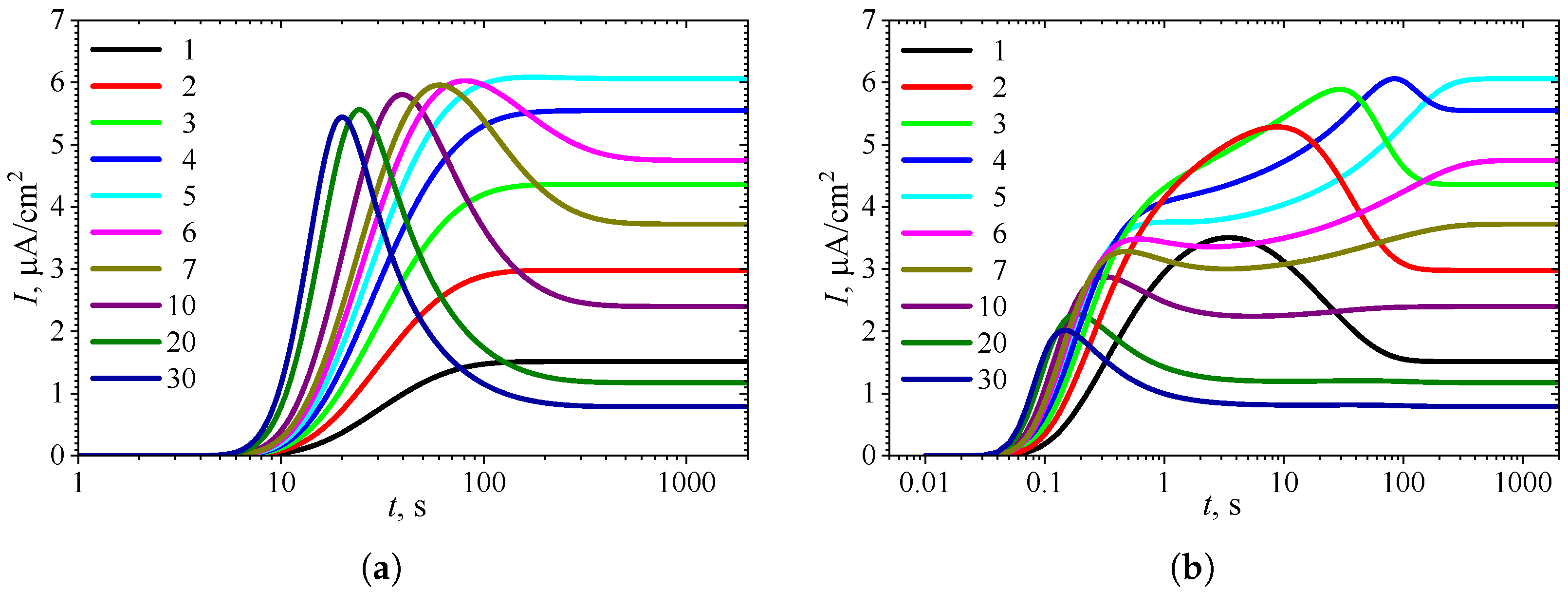
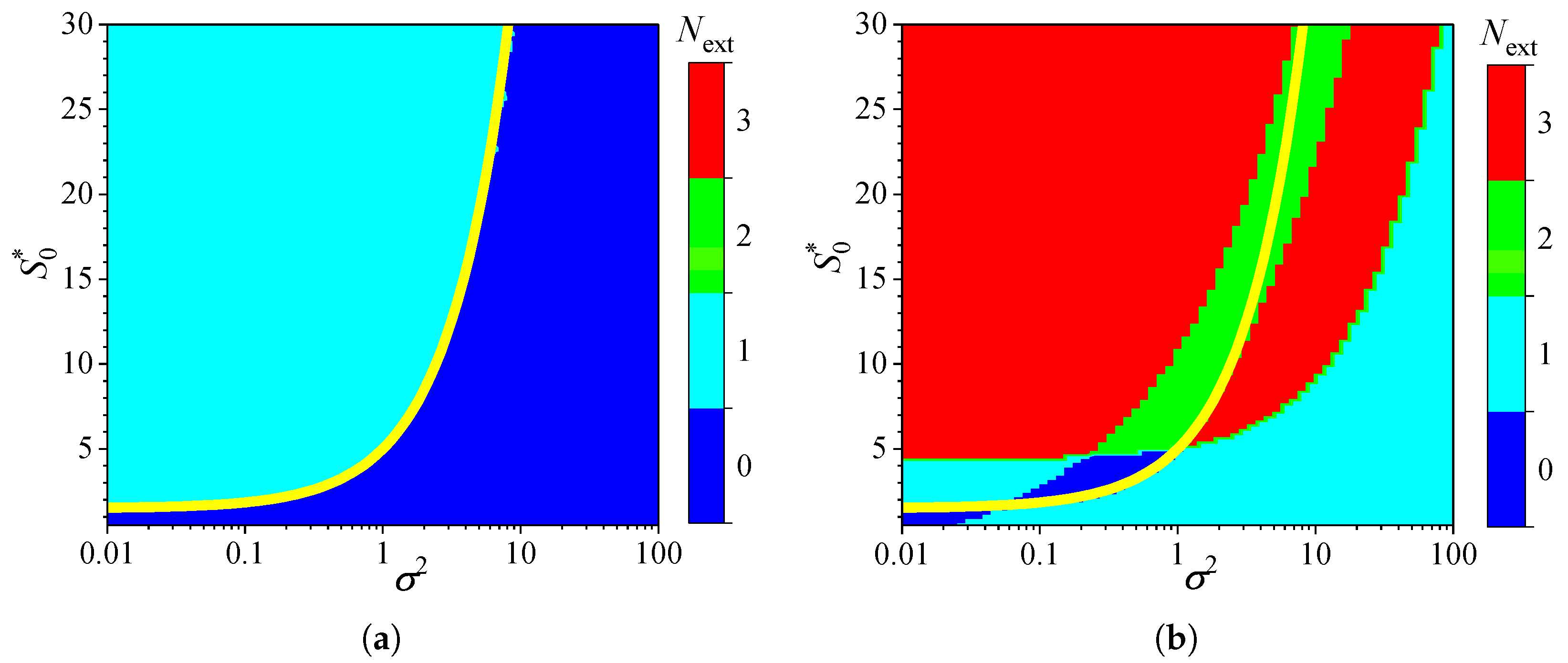
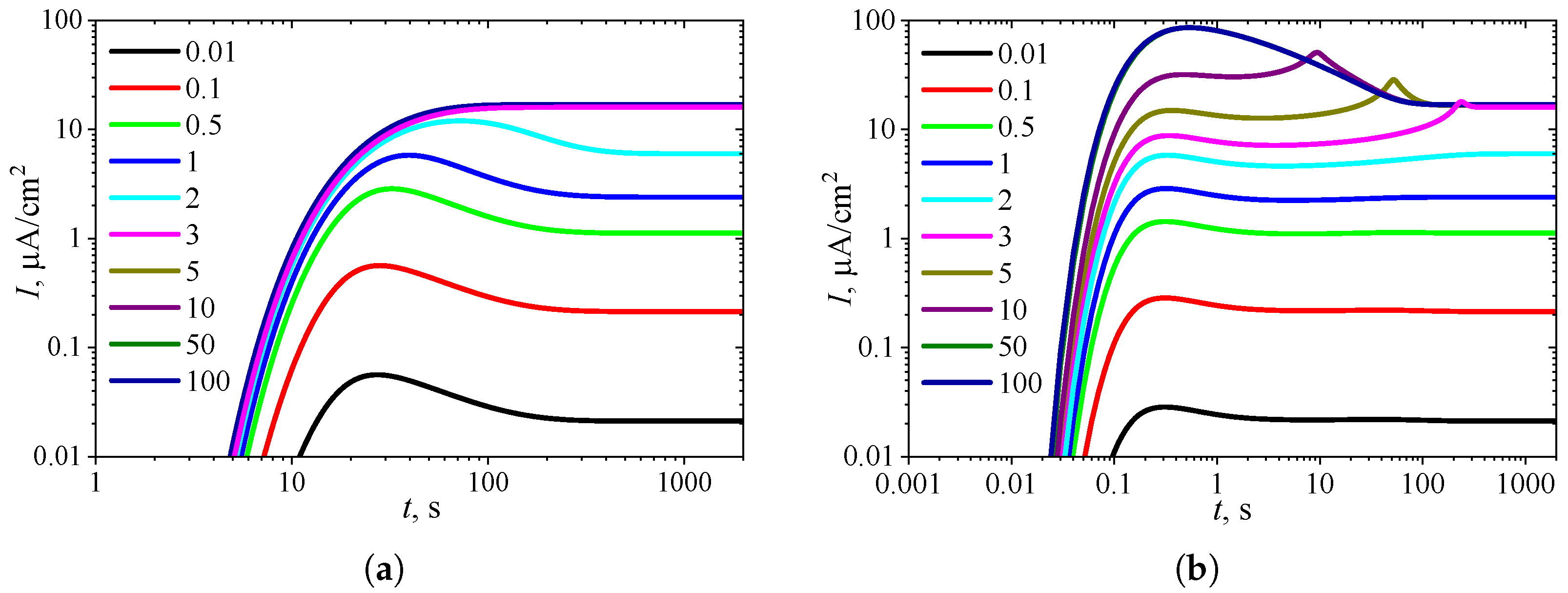
3.1. Temporal Dynamics of Biosensor Response

Figure 2 shows the typical temporal dynamics of the biosensor current I, simulated under uncompetitive substrate inhibition ($K_I^{\prime }=\infty$) at the following ten initial substrate concentrations $S_0$: 0.1, 0.2, 0.3, 0.4, 0.5, 0.6, 0.7, 1, 2, and 3 $\mathrm{mM}$. The simulations were performed using fixed parameters: $V_{max}$ = $100\mathrm{\mu }\mathrm{M}/\mathrm{s}$, $\theta$ = $0.75$, and $K_I=K_M$, in both types of analysis, injection analysis (IA) and batch analysis (BA). The corresponding normalized values $S_0^{*}=S_0/K_M$ of the substrate concentration are indicated on the curves in Figure 2. All the other model parameters were defined in (19). These simulations were performed under mixed control, involving both enzyme kinetics and internal diffusion (${\sigma }^2=1$). On the other hand, mass transport in the outer diffusion layer was slower than in the enzyme layer, as indicated by $\beta =0.13$.

One can see a noticeable difference in the dynamics of the biosensor response in Figure 2 when changing the substrate concentration $S_0$. The shape of the curves also depends significantly on the mode of analysis, i.e., on the initial conditions (13) or (14). However, the steady-state response is independent of the analysis mode, as the steady-state solution of the initial boundary value problem (8)–(11) is unaffected by those initial conditions [8,30,39,60].

At the beginning of biosensor operation, the output current becomes noticeably slower in IA mode than in BA mode. The delay consists of about 6–10 s. This delay in the transient response can be attributed to the diffusion time required for the substrate to pass through the outer diffusion layer and reach the enzyme layer in IA mode [4,34,64]. In contrast, in BA, the substrate contacts the enzyme layer immediately at $t=0$. The corresponding steady-state times are approximately the same, though they noticeably depend on the substrate concentration.

In IA (Figure 2a), at relatively high substrate concentrations ($S_0^{*}>5$), the response follows a three-phase pattern: starting from zero, reaching a maximum, and finally decreasing to a steady value. The output current, after reaching its maximum, enters the descending limb of the bell-shaped curve characteristic of uncompetitive substrate inhibition. In the case of low and moderate substrate concentrations ($S_0^{*}\le 5$ in Figure 2a), the biosensor current monotonically approaches steady-state. On the other hand, Figure 2a shows nonmonotonic behavior of the steady-state current. At substrate concentrations corresponding to the three-phase pattern ($S_0^{*}>5$), the steady-state current decreases with increasing $S_0^{*}$, whereas at lower concentrations ($S_0^{*}\le 5$), it increases with increasing $S_0^{*}$. These aspects of the biosensor with uncompetitive substrate inhibition are well known [24,31,35,36,37,38].

In particular, Forastiere et al. determined that the maximal steady-state current can be achieved at relatively low substrate concentration due to substrate inhibition, and that it can be several times greater than the current observed at extremely high substrate concentrations [24], consistent with the simulation results presented in Figure 2. Rafat et al. have demonstrated a nonmonotonic dependence of the biosensor response and sensitivity on the substrate concentration and mass transfer for IBE biosensors and an amperometric electrochemical immunosensor [10,58]. Sánchez-Trasviña et al. demonstrated how the appearance of substrate inhibition transforms the monotonically increasing reaction rate versus luminol concentration into a nonmonotonic behavior [65].

Figure 2b shows noticeably more complex dynamics of the biosensor current in BA mode than in IA. Even at relatively low substrate concentrations ($1\le S_0^{*}\le 4$), the output current is nonmonotonic. At a slightly greater concentration $S_0^{*}=5$, the output current becomes a monotonously increasing function of time t, butit has an extra inflection point ($t\approx 2$ s) where the curve changes from concave down to concave up.

In the case of relatively high substrate concentrations ($6\le S_0^{*}\le 10$), the biosensor response exhibits a local minimum and follows a four-phase pattern. At higher concentrations $S_0^{*}\ge 20$, the response even approaches a five-phase pattern, although the oscillations at $t>10$ are only slight. Specifically, at $S_0^{*}=20$, the transient current $I\left(t\right)$ starts from zero, reaches a global maximum of $2.27\mathrm{\mu }\mathrm{A}/\mathrm{c}{\mathrm{m}}^2$ at $t=0.18$ s, decreases to a local minimum of $1.196\mathrm{\mu }\mathrm{A}/\mathrm{c}{\mathrm{m}}^2$ at $t=10.5$ s, increases to a local maximum of $1.206\mathrm{\mu }\mathrm{A}/\mathrm{c}{\mathrm{m}}^2$ at $t=42$ s, and finally decreases to a steady value of $1.17\mathrm{\mu }\mathrm{A}/\mathrm{c}{\mathrm{m}}^2$. Thus, the variation between the local extrema and the steady value is only 2–3%. At a higher concentration of $S_0^{*}=30$, this variation is even smaller.

3.2. Effect of Internal Diffusion Limitation

Figure 2 shows the influence of substrate concentration on the dynamics of output current at a fixed maximal enzymatic rate of $V_{max}$ = $100\mathrm{\mu }\mathrm{M}/\mathrm{s}$, which corresponds to a diffusion module equal to unity (${\sigma }^2=1$). To investigate the effect of the diffusion module on the transient response of the amperometric biosensors, the response was simulated at very different values of $V_{max}$. This allowed the transition from enzyme kinetics control (${\sigma }^2\ll 1$) to internal diffusion control (${\sigma }^2\gg 1$) to be observed, while keeping all other parameters the same as those used in the simulations depicted in Figure 2. Figure 3 shows the number $N_{\mathrm{ext}}$ of extrema calculated from the simulated responses in both modes of analysis, IA and BA.

As shown in Figure 3a, the transient output current exhibits one or even no local extrema in IA, when the diffusion module changes in four orders of magnitude, from $0.01$ to 100, and the dimensionless substrate concentration $S_0^{*}$ changes from 1 to 30. When the biosensor acts under the internal diffusion limitation (${\sigma }^2\gg 1$), the response follows a two-phase pattern ($N_{\mathrm{ext}}=0$): starting from zero increases to a steady value. A three-phase pattern ($N_{\mathrm{ext}}=1$) is observed when the biosensor response is governed by enzyme kinetics or mixed control (${\sigma }^2\lesssim 10$), although it also depends on the substrate concentration. The yellow line in Figure 3 represents an approximate boundary between the two values of $N_{\mathrm{ext}}$, 0 and 1, i.e., between model parameter values that result in either two-phase or three-phase patterns. This yellow line is a linear approximation of the boundary,

$$S_0^{*}=1.5+3.5{\sigma }^2.$$

(20)

The relationship (20) between the substrate concentration and the diffusion module ${\sigma }^2$, resulting in changes in the number of response phases, is approximately linear when the biosensor operates in IA mode, as defined by (20) (Figure 3a). Similar dependencies of the substrate concentration on the diffusion module have already been observed [31,36,38,44,45]. In particular, it was found that the minimum dimensionless substrate concentration at which the response reaches its maximum is a monotonically increasing function of ${\sigma }^2$ [36]. In the case of BA (Figure 3b), that relation is noticeably more complicated as the number $N_{\mathrm{ext}}$ of extrema varies between zero and three, indicating that the number of phases in the response pattern ranges between two and five. In particular, at ${\sigma }^2=1$, increasing the normalized substrate concentration $S_0^{*}$ from 1 to 30 results in the number $N_{\mathrm{ext}}$ of extrema changing in the following sequence: 1, 0, 1, 2, 3. This can also be noticed in Figure 2b.

Although the variation in the number of extrema $N_{\mathrm{ext}}$ differs noticeably among the analysis modes, at relatively low substrate concentrations ($S_0^{*}\lesssim 4.5$) and very low values of the diffusion module (${\sigma }^2\lesssim 0.03$), the number $N_{\mathrm{ext}}$ is practically invariant across the analysis mode, as observed in the lower left corners of Figure 3a,b.

To observe the effect of the diffusion module ${\sigma }^2$ on the shape of the transient response, the biosensor action was simulated at different values of ${\sigma }^2$ while keeping the substrate concentration fixed at a relatively high level ($S_0^{*}$ = $10K_I^{*}$ = 10, $S_0=10K_I$), where the uncompetitive inhibition plays a significant role in the biosensor response. The simulation results are shown in Figure 4.

One can see in Figure 4a that in IA, the transient output current exhibits a global maximum for ${\sigma }^2<3$, whereas it is a monotonously increasing function of time t for greater values of the diffusion module ${\sigma }^2$, as predicted in Figure 3a. In BA (Figure 4b), for ${\sigma }^2<3$, the shape of $I\left(t\right)$ is similar to that observed in the IA mode (Figure 4a), although the function $I\left(t\right)$ in BA has additional local extrema, which are close to steady values. However, at slightly greater values of ${\sigma }^2$ ($3\le {\sigma }^2\le 10$), the transient current $I\left(t\right)$ exhibits a noticeable peak in BA. At high values of the diffusion module (${\sigma }^2>20$), when the response is governed by internal diffusion control, the output current exhibits only a global maximum, following a two-phase pattern.

On the other hand, at high values of the diffusion module (${\sigma }^2>5$), the transient response in IA becomes practically invariant to ${\sigma }^2$, whereas in BA, the response dynamics still noticeably depend on ${\sigma }^2$. Maintaining the analytical capability of biosensors for as long as possible is very important [2,4,7]. Typically, the maximal enzymatic rate $V_{max}$ decreases over time due to enzyme inactivation [76,88]. Therefore, ensuring the stability of the biosensor response (the biosensor resistance) across a range of $V_{max}$ values is crucial [30,38,42,44,45,88]. Since $V_{max}$ directly influences ${\sigma }^2$, it is essential to maintain a stable response even when ${\sigma }^2$ undergoes slight variations.

In particular, at two significantly different values of ${\sigma }^2$, namely $0.5$ and 5, the response of a biosensor operating under BA conditions follows a five-phase pattern ($N_{\mathrm{ext}}$ = 3). However, in the case of ${\sigma }^2=0.5$ (and for ${\sigma }^2<0.5$ as well), the local minimum is barely noticeable, whereas for ${\sigma }^2=5$, all extrema and all five phases are clearly observable. This is particularly important in practical applications of amperometric biosensors, as oscillations in the biosensor response may complicate the use of the calibration curve [21,22]. On the other hand, analyzing both the steady-state and the maximal biosensor currents can significantly extend the calibration curve when using intelligent biosensors [21,35,36,89].

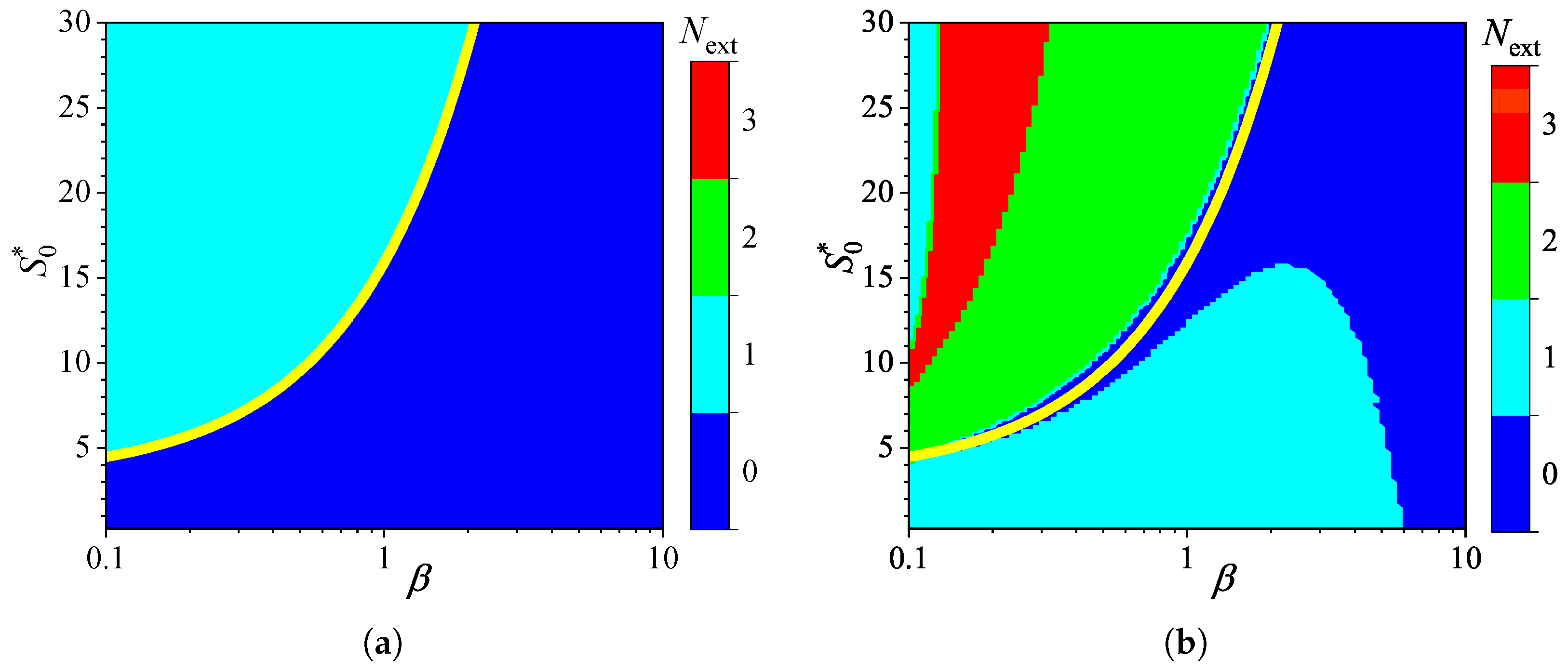
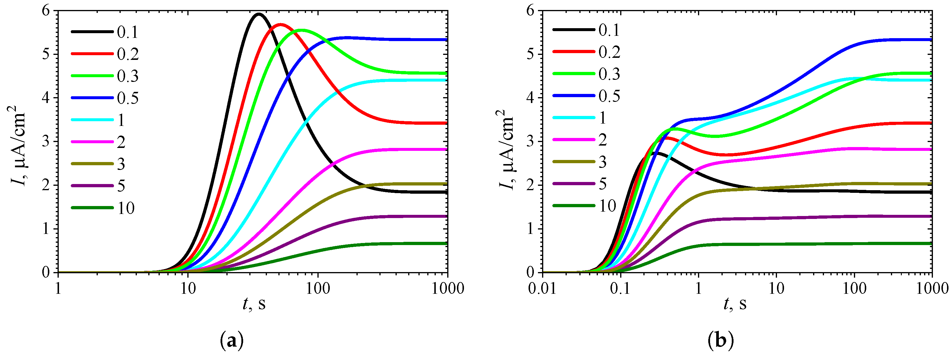
3.3. Effect of External Diffusion Limitation

To investigate the influence of external diffusion limitations on the behavior of amperometric enzyme-based biosensors, the biosensor response was simulated by varying the partition coefficient $\theta$ over two orders of magnitude, from $0.01$ to $1.0$. This variation caused the governing dimensionless Biot number $\beta$ to change from $0.1$ to 10, representing a shift from external to internal mass transfer dominance [9,78]. The substrate concentration $S_0$ was also independently varied from 0.025 to 3 mM. Simulations were conducted for both types of analysis, injection (IA) and batch (BA), using fixed parameters of $V_{max}$ = $100\mathrm{\mu }\mathrm{M}/\mathrm{s}$ and $K_I=K_M$. Figure 5 shows the number $N_{\mathrm{ext}}$ of extrema calculated from the simulated responses.

As one can see in Figure 5a, in IA, the dependence of the number $N_{\mathrm{ext}}$ of extrema of the transient current on the Biot number is rather similar in shape to that on the diffusion module ${\sigma }^2$. In IA, when the mass transport by diffusion in the diffusion layer is notably faster than in the enzyme layer ($\beta \gtrsim 2$), the response follows a two-phase pattern ($N_{\mathrm{ext}}=0$). At smaller values of $\beta$, when the diffusion in the outer diffusion layer is comparable with or slower than that in the enzyme layer ($\beta \lesssim 1$), the response follows a three-phase pattern ($N_{\mathrm{ext}}=1$), although it also depends on the substrate concentration. The yellow line in Figure 5a represents an approximate boundary between the two values of $N_{\mathrm{ext}}$, 0 and 1,

$$S_0^{*}=3.2+12.7\beta .$$

(21)

In the case of BA (Figure 5b), the relationship between the number $N_{\mathrm{ext}}$ of extrema, the Biot number $\beta$, and the substrate concentration is noticeably more complex. The number $N_{\mathrm{ext}}$ varies between zero and three, and the boundary between the regions where $N_{\mathrm{ext}}=0$ and $N_{\mathrm{ext}}=1$ is clearly nonlinear. Nevertheless, the boundary (yellow line) between areas indicated as $N_{\mathrm{ext}}=0$ and $N_{\mathrm{ext}}=2$ is similar to that observed in IA (Figure 5a) between $N_{\mathrm{ext}}=0$ and $N_{\mathrm{ext}}=1$. At relatively high substrate concentrations ($S_0^{*}\gtrsim 15$), the number of response phases is the same in both modes of analysis, IA and BA, except when $0.15\lesssim \beta \lesssim 2$, where the number of phases in BA is greater than in IA.

To observe the effect of the Biot number $\beta$ on the shape of the transient response, the biosensor performance was simulated at nine values of $\beta$, while keeping the substrate concentration fixed at a relatively high level ($S_0^{*}$ = $10K_I^{*}$ = 10). The simulation results are shown in Figure 6.

Figure 6a shows that in IA at $S_0^{*}=10$, the transient biosensor current exhibits a global maximum for $\beta \le 0.5$, whereas it is a monotonously increasing function of time t for greater values of the Biot number $\beta$, as also shown in Figure 5a.

In BA (Figure 6b), three extrema can be observed only for the smallest value of the Biot number of $\beta =0.1$. However, a local minimum and local maximum differ by less than 1 percent. At $\beta =0.5$, no local extrema are observed, but an extra inflection point ($t\approx 2$ s) is observed where the curve changes from concave down to concave up. When $1\le \beta \le 3$, the transient output current has only one global maximum ($N_{\mathrm{ext}}=1$), which occurs noticeably later (at $t\approx 100$ s) than the global maximum observed for small values of $\beta$ (at $t<1$ s), and is close to the steady-state value. For larger values of $\beta$ ($\beta >3$), the global maximum decreasingly approaches the steady-state value.

In addition to the Biot number $\beta$, the external Thiele modulus ${\sigma }_{\mathrm{ext}}$ (also known as the external Damköhler number and the external diffusion module) is used to compare external and internal mass transport resistances. It relates the characteristic timescale of the enzymatic reaction within the enzyme layer to that of external mass transfer, i.e., it represents the ratio between the first-order surface reaction rate ($V_{max}{\theta }_S/K_M{d}_1$) and the rate of the mass transfer through the external diffusion layer ($D_{S_2}/d_2$) [22,35,49,50]. If ${\sigma }_{\mathrm{ext}}^2\ll 1$, then the external mass transfer is fast, and the system acts in a reaction-limited regime. The enzymatic reaction is fast, and the external diffusion is limiting when ${\sigma }_{\mathrm{ext}}^2\gg 1$. The internal and external Thiele moduli are related through the Biot number for the mass transfer,

$${\sigma }_{\mathrm{ext}}^2={\displaystyle \frac{V_{max}{\theta }_S{d}_1{d}_2}{K_M{D}_{S_2}}}={\displaystyle \frac{{\sigma }^2}{{\beta }_S}}.$$

(22)

The effect of the external Thiele modulus on the behavior of amperometric enzyme-based biosensors was not investigated separately, as it is represented through two other dimensionless parameters: the diffusion module ${\sigma }^2$ and the Biot number $\beta$ = ${\beta }_S$.

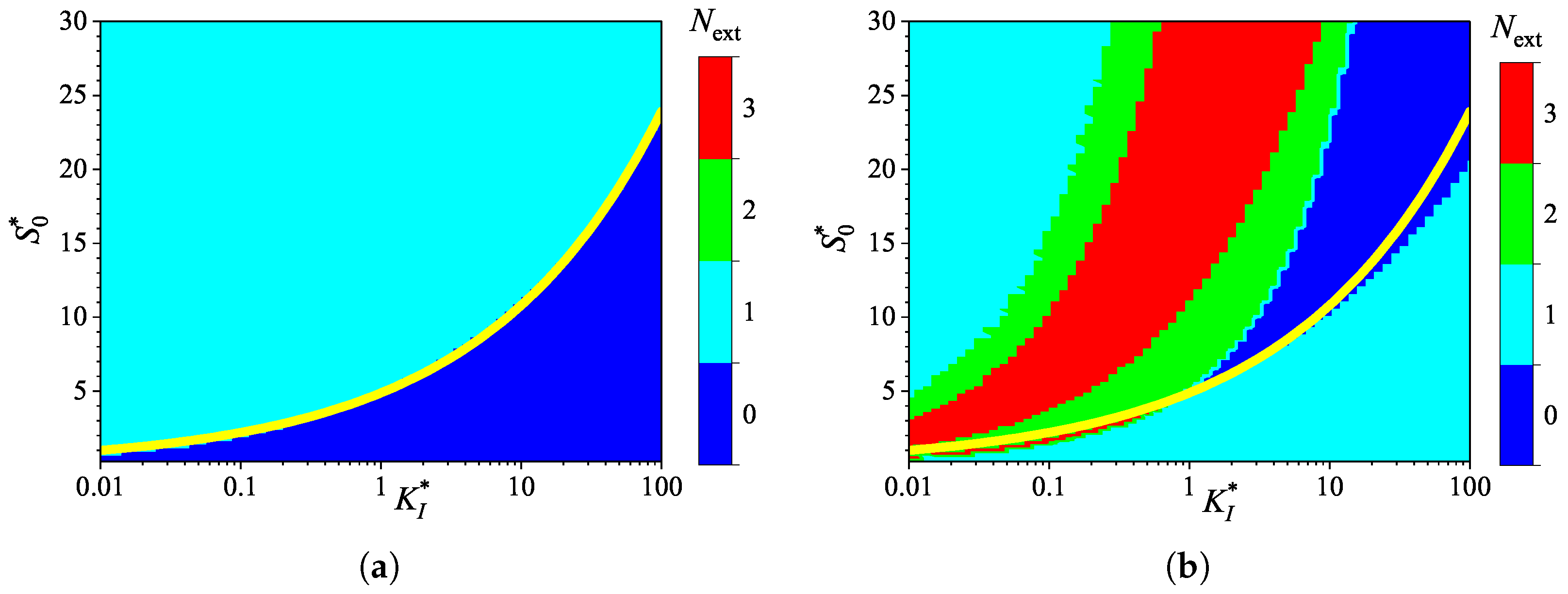
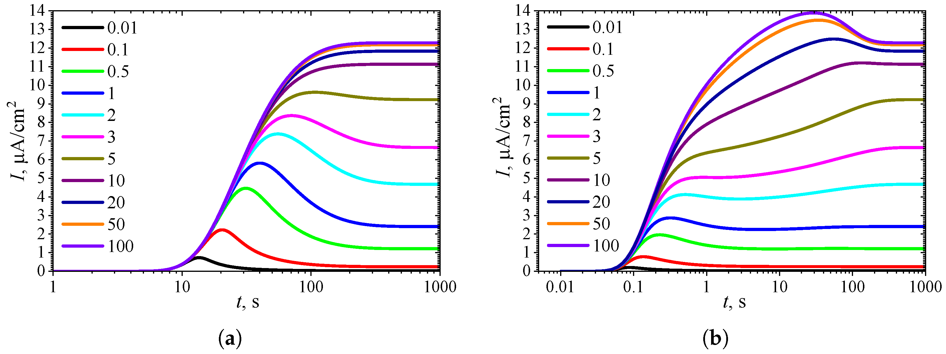
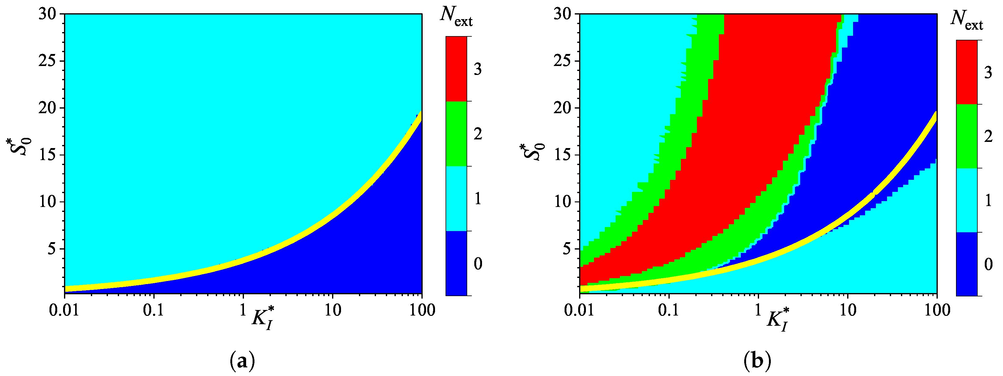
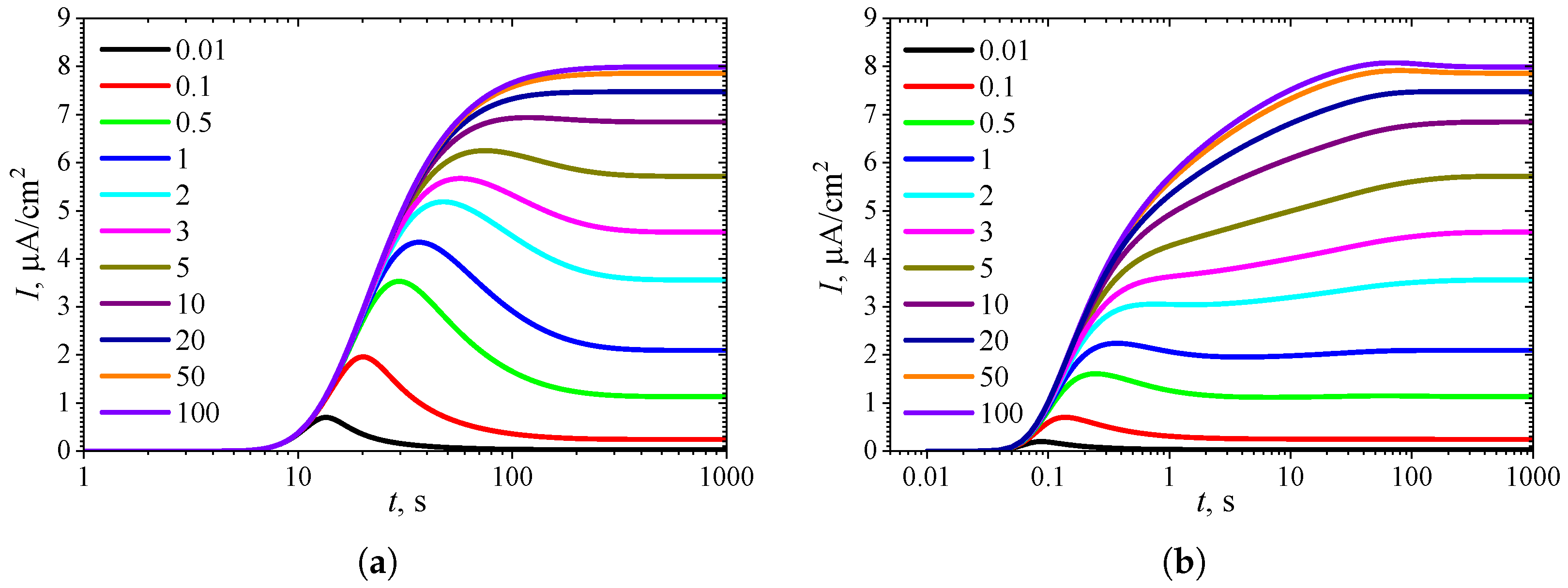
3.4. Effect of Uncompetitive Substrate Inhibition

To investigate the effect of uncompetitive substrate inhibition ($K_I^{\prime }=\infty$) on the behavior of the biosensor transient current, the biosensor response was simulated by varying the inhibition constant $K_I$ over four orders of magnitude, from $1\mathrm{\mu }\mathrm{M}$ to $10\mathrm{m}\mathrm{M}$, thereby changing the normalized inhibition constant $K_I^{*}$ from $0.01$ to 100. The substrate concentration $S_0$ was independently varied from 0.025 to 3 mM, as in the numerical experiments discussed above. Simulations were conducted for both types of analysis, injection (IA) and batch (BA), using fixed parameters of $V_{max}$ = $100\mathrm{\mu }\mathrm{M}/\mathrm{s}$ and $\theta =0.75$. At these parameter values, the diffusion module ${\sigma }^2=1$, and the Biot number $\beta =0.13$. Figure 7 shows the calculated number $N_{\mathrm{ext}}$ of extrema.

As shown in Figure 7, the dependence of the number $N_{\mathrm{ext}}$ of extrema of the transient current on the inhibition constant $K_I^{*}$ differs noticeably from those on the diffusion module ${\sigma }^2$ (Figure 3) and the Biot number $\beta$ (Figure 5).

In IA (Figure 7a), the response follows a three-phase pattern ($N_{\mathrm{ext}}=1$) in most of the entire region of parameter values, $(S_0^{*},K_I^{*})\in$$[0.25,30]\times [0.01,100]$. Only at relatively low substrate concentrations and large values of the inhibition constant, the response follows a two-phase pattern ($N_{\mathrm{ext}}=0$), as in the Michaelis–Menten kinetics. This behavior is reasonable because the influence of inhibition decreases with an increasing inhibition constant $K_I^{*}$. Nevertheless, an increase in the inhibition constant can be compensated for by an increase in the substrate concentration. In a particular case of $K_I^{*}=10$, the inhibitory term $S^2/K_I$ in the reaction rate Equation (5) becomes significant when $S_0^{*}\ge K_I^{*}$. The relationship between $S_0^{*}$ and $K_I^{*}$ is nonlinear. The yellow line in Figure 7a represents an approximate boundary between the two values of $N_{\mathrm{ext}}$, 0 and 1. This line is a power-law (allometric) approximation of the boundary,

$$S_0^{*}=4.9\times {K_I^{*}}^{0.345}.$$

(23)

As shown in Figure 7, in the region parameter values $S_0^{*}$ and $K_I^{*}$ where $N_{\mathrm{ext}}=0$ in IA (i.e., below the yellow line), $N_{\mathrm{ext}}=1$ in BA.

Figure 7a shows that, in the particular case of $K_I^{*}=1$, the transient output current in IA is a monotonically increasing function of time for concentrations $S_0^{*}\lesssim 5$, and become a non-monotonic function (with $N_{\mathrm{ext}}=1$) at higher concentrations. In the corresponding BA (Figure 7b), the number $N_{\mathrm{ext}}$ changes with increasing substrate concentration in the following sequence: 1, 0, 2, 3. Notably, $N_{\mathrm{ext}}=0$ occurs in the specific case of $S_0^{*}=5$. The current dynamics in these cases are also illustrated in Figure 2.

To observe the effect of the inhibition constant $K_I^{*}$ on the dynamics of the transient current, the biosensor action was simulated at eleven different $K_I^{*}$ values, with the constant substrate concentration held at $S_0^{*}$ = 10. The simulation results are depicted in Figure 8.

As seen in Figure 7a and Figure 8a, in IA at $S_0^{*}=10$, the transient current exhibits a global maximum for all values of the inhibition constant $K_I^{*}$ less than 8. Only when $K_I^{*}$ becomes comparable to or greater than the concentration $S_0^{*}$ ($K_I^{*}\gtrsim S_0^{*}$) does the output current become a monotonically increasing function of time t.

In BA (Figure 6b and Figure 7b), the transient current at $S_0^{*}=10$ is monotonic only within a relatively narrow range of the inhibition constant $K_I^{*}$, approximately between 3 and 8. The number of extrema $N_{\mathrm{ext}}=3$ is observed when $K_I^{*}$ varies approximately between 0.1 and 0.9. However, the local minimum and maximum differ from the steady-state by only 1–2%, although the global maximum is noticeably more pronounced. Such small deviations in local extrema from the steady value can be considered perturbations of the response, influencing the response analysis procedure [21,35,36,89].

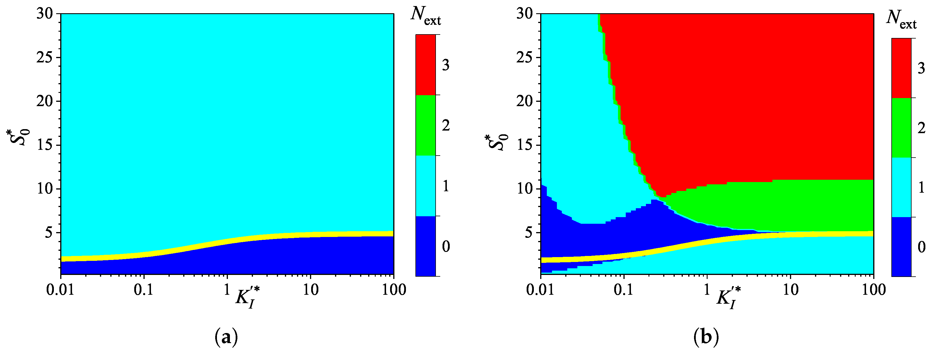
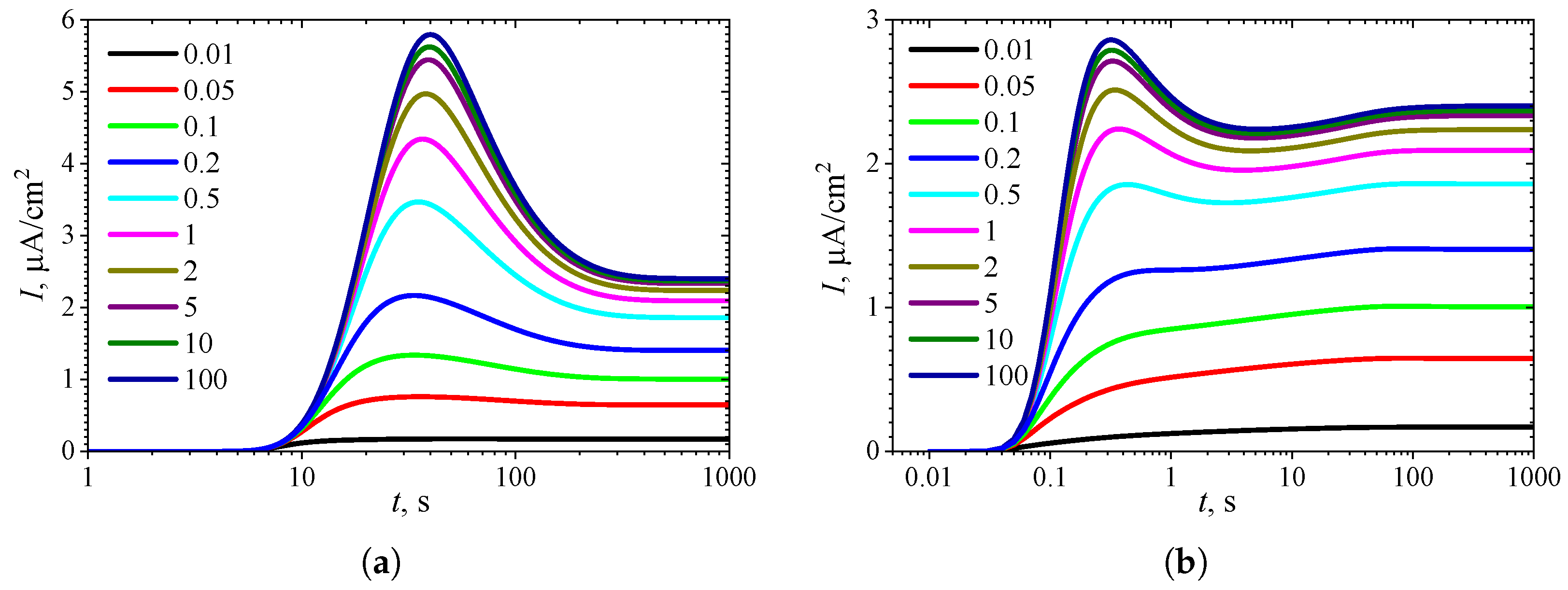
3.5. Effect of Noncompetitive Substrate Inhibition

To examine the impact of noncompetitive substrate inhibition on the transient current behavior of the biosensor, the response was simulated by varying both the uncompetitive ($K_I$ ) and competitive ($K_I^{\prime }$) inhibition constants. All other parameters were the same as those used in the analysis of uncompetitive substrate inhibition presented earlier in this section. The simulation results are presented in Figure 9, Figure 10, Figure 11 and Figure 12. Figure 9 and Figure 11 display the computed number $N_{\mathrm{ext}}$ of extrema, while Figure 10 and Figure 12 show the dynamics of the output current $I\left(t\right)$.

The numerical experiments whose results are presented in Figure 9 and Figure 10 differ from those shown in Figure 7 and Figure 8 only in the values of the competitive inhibition constant $K_I^{\prime }$. Figure 9 and Figure 10 illustrate how the response of the biosensor, operating under uncompetitive substrate inhibition, is influenced by the addition of competitive substrate inhibition at a fixed moderate rate $K_I^{\prime }=K_M$; that is, how the competitive substrate inhibition reaction (3) affects the response of the biosensor governed by reactions (1) and (2).

One can observe similar shapes in the evolution of output current $I\left(t\right)$ in Figure 8 and Figure 10, but there is a noticeable difference in its absolute values. However, this difference becomes significant only when the uncompetitive inhibition constant $K_I$ exceeds the Michaelis constant ($K_I>K_M$, $K_I^{*}>1$). At $K_I^{*}=0.1$ ($K_I=0.1K_M$), the steady-state output current $I_{\mathrm{ss}}$ in the case of noncompetitive substrate inhibition (Figure 10) is only about 1% lower than that for uncompetitive substrate inhibition (Figure 8). This difference increases with increasing substrate concentration $S_0$, reaching 12% at $K_I^{*}=1$ and 35% at $K_I^{*}=100$. This property is valid for both IA and BA analysis modes.

The increasing influence of the competitive inhibition constant $K_I^{\prime }$ while increasing the uncompetitive inhibition constant $K_I$ can also be observed in the dependence of the number $N_{\mathrm{ext}}$ of extrema in the biosensor current on the normalized inhibition constant $K_I^{*}$ and the substrate concentration $S_0^{*}$ (Figure 7 and Figure 9). The corresponding regions with the same number $N_{\mathrm{ext}}$ have very similar shapes for $K_I^{*}<1$, but they diverge for larger values of $K_I^{*}$. Similar to the case of uncompetitive inhibition, the boundary between the two values of $N_{\mathrm{ext}}$, 0 and 1, observed in the IA mode for noncompetitive inhibition and indicated by the yellow line in Figure 9a, is also approximated by a power-law (allometric) relationship,

$$S_0^{*}=3.81\times {K_I^{*}}^{0.354}.$$

(24)

The increasing effect of the competitive inhibition constant $K_I^{\prime }$ with an increasing uncompetitive inhibition constant $K_I$ can be explained by the reaction rate expression (5). At a fixed value of $K_I^{\prime }$, the rate of the noncompetitive (mixed) inhition $V\left(S\right)$ approaches the rate of competitive inhibition, as defined in (7), when $K_I\gg K_I^{\prime }$.

To extend the study of the impact of noncompetitive substrate inhibition on the transient current behavior of the biosensor, the response was simulated by varying the competitive ($K_I^{\prime }$), keeping the uncompetitive ($K_I$ ) inhibition constants unchanged. Figure 11 shows the dependence of the number $N_{\mathrm{ext}}$ of extrema in the biosensor current on the normalized inhibition constant $K_I^{*}$ and the normalized substrate concentration $S_0^{*}$, with a fixed competitive substrate inhibition constant $K_I^{\prime }=K_M$ for the IA (a) mode and BA (b) mode.

As one can see in Figure 11a, in IA, the dependence of the number $N_{\mathrm{ext}}$ of extrema of the transient current on the normalized competitive inhibition constant ${K_I^{\prime }}^{*}$ noticeably differs in shape from the dependencies observed earlier in this section. The yellow line in Figure 11a, representing an approximate boundary between the two values of $N_{\mathrm{ext}}$, 0 and 1, saturates as ${K_I^{\prime }}^{*}\to \infty$ and is expressed as a rational function,

$$S_0^{*}=4.9-{\displaystyle \frac{1.3}{0.44+{K_I^{\prime }}^{*}}}.$$

(25)

Figure 11b shows a relatively large region where $N_{\mathrm{ext}}=3$ in BA. However, this region corresponds to only relatively high substrate concentrations ($S_0^{*}\gtrsim 10$). At $S_0^{*}=10$, Figure 12b clearly shows local minima and maxima for ${K_I^{\prime }}^{*}>0.2$ ($N_{\mathrm{ext}}=2$). The difference in maximal currents between the analysis modes is among the most significant differences observed, as shown in (Figure 12), compared to the other cases presented in Figure 2, Figure 4, Figure 6, Figure 8 and Figure 10.

When ${K_I^{\prime }}^{*}\gg 1$, at a fixed value of $K_I^{*}$, the rate of noncompetitive (mixed) inhibition $V\left(S\right)$ approaches the rate of uncompetitive inhibition, as defined in (6). Thus, at ${K_I^{\prime }}^{*}=100$, the simulation results shown in Figure 11 and Figure 12 for ${K_I^{\prime }}^{*}=100$ coincide with the results presented in Figure 7 and Figure 8 for the specific value $K_I^{*}=1$. In particular, the output currents in Figure 12, labeled with 100, coincide with the currents in Figure 8, labeled with 1, as in both cases $K_I^{*}=1$ ($K_I=K_M$).

4. Conclusions

The two-compartment mathematical model (8)–(14) of amperometric enzyme-based biosensors is useful for investigating the influence of noncompetitive (mixed) substrate inhibition, in conjunction with internal and external diffusion limitations, on the biosensor response. Deriving the corresponding dimensionless form of the model (A1)–(A7) reveals the main governing dimensionless parameters (18).

The dynamics of the enzymatic system shown in Figure 1 are highly sensitive to internal and external diffusion limitations, enzyme inhibition, and, most notably, the mode of analysis. In injection analysis (IA, real-time monitoring), where the arrival of the analyte initiates the biosensor transient response, the response follows a two- or three-phase pattern. In batch analysis (BA), where the biosensor is directly immersed in a buffer solution containing the analyte, the response may exhibit up to five phases. The number $N_{\mathrm{ext}}$ of extrema in the transient output current, as defined by Equation (17), is useful for determining the conditions under which the biosensor response follows a multi-phase pattern. The steady-state biosensor current is invariant with respect to the analysis mode (Figure 2, Figure 4, Figure 6, Figure 8, Figure 10 and Figure 12).

The non-monotonic (three-phase, $N_{\mathrm{ext}}=1$) transient output current of biosensors operating in IA is observed only when the enzyme kinetics predominate in the biosensor response, compared to the internal diffusion, or when the operation is under mixed control (diffusion module ${\sigma }^2\lesssim 10$) (Figure 3a), the diffusion in the outer diffusion layer is comparable to or slower than that in the enzyme layer (the Biot number $\beta \lesssim 1$) (Figure 5a), and the substrate concentration is comparable to or greater than the inhibition constant (Figure 7a), where the current shows a global maximum greater than a steady value (Figure 4a, Figure 6a and Figure 8a).

In BA, the monotonic (two-phase, $N_{\mathrm{ext}}=0$) transient current is observed only when the biosensor response is notably governed by enzyme kinetics (${\sigma }^2<1$), mass transport by diffusion in the diffusion layer is faster than in the enzyme layer ($\beta \gtrsim 1$), and under specific values of other parameters. Under conditions where biosensors operating in IA follow a three-phase pattern, the transient current in BA can exhibit a maximum five-phase pattern ($N_{\mathrm{ext}}=3$) (Figure 3b, Figure 5b, and Figure 7b), where the current shows a global maximum, a local minimum, and a local maximum. The global maximum may occur either before or after a local minimum (Figure 4b, Figure 6b, and Figure 8b).

The effect of the competitive substrate inhibition constant $K_I^{\prime }$ on the response dynamics of biosensors operating under noncompetitive (mixed) substrate inhibition increases with increasing uncompetitive inhibition constant $K_I$ (Figure 9, Figure 10, Figure 11 and Figure 12).

Oscillations in the transient biosensor response, caused by substrate inhibition and both internal and external diffusion limitations, should be taken into consideration when using the biosensor calibration curve.

References

1. Bisswanger, H. Enzyme Kinetics: Principles and Methods, 2nd ed.; Wiley-Blackwell: Weinheim, Germany, 2008. [Google Scholar]
2. Malhotra, B.D.; Pandey, C.M. Biosensors: Fundamentals and Applications; Smithers Rapra: Shawbury, UK, 2017. [Google Scholar]
3. Patra, S.; Kundu, D.; Gogoi, M. (Eds.) Enzyme-based Biosensors: Recent Advances and Applications in Healthcare; Springer: Singapore, 2023. [Google Scholar]
4. Scheller, F.W.; Schubert, F. Biosensors; Elsevier Science: Amsterdam, The Netherlands, 1992. [Google Scholar]
5. Sadana, A.; Sadana, N. Handbook of Biosensors and Biosensor Kinetics; Elsevier: Amsterdam, The Netherlands, 2011. [Google Scholar]
6. Cornish-Bowden, A. Fundamentals of Enzyme Kinetics, 3rd ed.; Portland Press: London, UK, 2004. [Google Scholar]
7. Turner, A.P.F.; Karube, I.; Wilson, G.S. (Eds.) Biosensors: Fundamentals and Applications; Oxford University Press: Oxford, UK, 1990. [Google Scholar]
8. Bartlett, P.N. Bioelectrochemistry: Fundamentals, Experimental Techniques and Applications; John Wiley & Sons: Chichester, UK, 2008. [Google Scholar]
9. Banica, F.G. Chemical Sensors and Biosensors: Fundamentals and Applications; John Wiley & Sons: Chichester, UK, 2012. [Google Scholar]
10. Rafat, N.; Satoh, P.; Worden, R.M. Electrochemical Biosensor for Markers of Neurological Esterase Inhibition. Biosensors 2021, 11, 459. [Google Scholar] [CrossRef] [PubMed]
11. Gullo, L.; Brunelleschi, B.; Duranti, L.; Fiore, L.; Mazzaracchio, V.; Arduini, F. 3D printed shamrock-like electrochemical biosensing tool based on enzymatic inhibition for on-line nerve agent measurement in drinking water. Biosens. Bioelectron. 2025, 282, 117471. [Google Scholar]
12. Cornish-Bowden, A. The origins of enzyme kinetics. FEBS Lett. 2013, 587, 2725–2730. [Google Scholar] [PubMed]
13. Dixon, M.; Webb, E.; Thorne, C.; Tipton, K. Enzymes, 3rd ed.; Longman: London, UK, 1979. [Google Scholar]
14. Yoshino, M.; Murakami, K. Analysis of the substrate inhibition of complete and partial types. SpringerPlus 2015, 4, 292. [Google Scholar]
15. Attaallah, R.; Amine, A. The Kinetic and Analytical Aspects of Enzyme Competitive Inhibition: Sensing of Tyrosinase Inhibitors. Biosensors 2021, 11, 322. [Google Scholar] [CrossRef]
16. Stoica, L.; Ruzgas, T.; Gorton, L. Electrochemical evidence of self-substrate inhibition as functions regulation for cellobiose dehydrogenase from Phanerochaete chrysosporium. Bioelectrochemistry 2009, 76, 42–52. [Google Scholar]
17. Musser, S.M.; Stowell, M.H.B.; Lee, H.K.; Rumbley, J.N.; Chan, S.I. Uncompetitive substrate inhibition and noncompetitive inhibition by 5-n-undecyl-6-hydroxy-4,7-dioxobenzothiazole (UHDBT) and 2-n-Nonyl-4-hydroxyquinoline-N-oxide (NQNO) is observed for the cytochrome bo(3) complex: Implications for a Q(H-2)-loop proton translocation mechanism. Biochemistry 1997, 36, 894–902. [Google Scholar]
18. Staniszewski, M. Theoretical analysis of inhibition effect on steady states of enzymatic membrane reactor with substrate and product retention for reaction producing weak acid. Desalination 2009, 249, 1190–1198. [Google Scholar]
19. Croce, R.A.J.; Vaddiraju, S.; Papadimitrakopoulos, F.; Jain, F.C. Theoretical analysis of the performance of glucose sensors with layer-by-layer assembled outer membranes. Sensors 2012, 12, 13402–13416. [Google Scholar]
20. Dagan, O.; Bercovici, M. Simulation tool coupling nonlinear electrophoresis and reaction kinetics for design and optimization of biosensors. Anal. Chem. 2014, 86, 7835. [Google Scholar]
21. Baronas, R.; Kulys, J.; Lančinskas, A.; Žilinskas, A. Effect of diffusion limitations on multianalyte determination from biased biosensor response. Sensors 2014, 14, 4634–4656. [Google Scholar] [CrossRef] [PubMed]
22. Kulys, J. Biosensor response at mixed enzyme kinetics and external diffusion limitation in case of substrate inhibition. Nonlinear Anal. Model. Control. 2006, 11, 385–392. [Google Scholar]
23. Mirón, J.; González, M.P.; Vázquez, J.A.; Pastrana, L.; Murado, M.A. A mathematical model for glucose oxidase kinetics, including inhibitory, deactivant and diffusional effects, and their interactions. Enzyme Microb. Technol. 2004, 34, 513–522. [Google Scholar]
24. Forastiere, D.; Falasco, G.; Esposito, M. Strong current response to slow modulation: A metabolic case-study. J. Chem. Phys. 2020, 152, 134101. [Google Scholar] [PubMed]
25. Boshagh, F.; Rostami, K.; van Niel, E.W. Application of kinetic models in dark fermentative hydrogen production—A critical review. Int. J. Hydrogen Energy 2022, 47, 21952–21968. [Google Scholar]
26. Meraz, M.; Alvarez-Ramirez, J.; Vernon-Carter, E.J.; Reyes, I.; Hernandez-Jaimes, C.; Martinez-Martinez, F. A Two Competing Substrates Michaelis-Menten Kinetics Scheme for the Analysis of In Vitro Starch Digestograms. Starch-Starke 2020, 72, 1900170. [Google Scholar]
27. Meriç, S.; Tünay, O.; San, H.A. A new approach to modelling substrate inhibition. Environ. Technol. 2002, 23, 163–177. [Google Scholar]
28. Meriç, S.; Tünay, O.T.; San, H.A. Modelling approaches in substrate inhibition. Fresenius Environ. Bull. 1998, 7, 183–189. [Google Scholar]
29. Zhang, S.; Zhao, H.; John, R. Development of a quantitative relationship between inhibition percentage and both incubation time and inhibitor concentration for inhibition biosensors-theoretical and practical considerations. Biosens. Bioelectron. 2001, 16, 1119–1126. [Google Scholar]
30. Baronas, R.; Ivanauskas, F.; Kulys, J. Mathematical Modeling of Biosensors; Springer Series on Chemical Sensors and Biosensors; Springer: Cham, Switzerland, 2021; Volume 9, p. 456. [Google Scholar]
31. Achi, F.; Bourouina-Bacha, S.; Bourouina, M.; Amine, A. Mathematical model and numerical simulation of inhibition based biosensor for the detection of Hg(II). Sens. Actuator B Chem. 2015, 207, 413–423. [Google Scholar]
32. Kernevez, J. Enzyme Mathematics. Studies in Mathematics and Its Applications; Elsevier Science: Amsterdam, The Netherlands, 1980. [Google Scholar]
33. Manimozhi, P.; Subbiah, A.; Rajendran, L. Solution of steady-state substrate concentration in the action of biosensor response at mixed enzyme kinetics. Sensor. Actuator B-Chem. 2010, 147. [Google Scholar]
34. Murray, J.D. Mathematical Biology: I. An Introduction, 3rd ed.; Springer: New York, NY, USA, 2002. [Google Scholar]
35. Kulys, J.; Baronas, R. Modelling of amperometric biosensors in the case of substrate inhibition. Sensors 2006, 6, 1513–1522. [Google Scholar] [CrossRef]
36. Šimelevičius, D.; Baronas, R. Computational modelling of amperometric biosensors in the case of substrate and product inhibition. J. Math. Chem. 2010, 47, 430–445. [Google Scholar]
37. Reed, M.C.; Lieb, A.; Nijhout, H.F. The biological significance of substrate inhibition: A mechanism with diverse functions. BioEssays 2010, 32, 422–429. [Google Scholar] [PubMed]
38. Mohanasundaraganesan, M.; Luis, J.; Guirao, G.; Rathinama, S. Theoretical Analysis of Amperometric Biosensor with Substrate and Product Inhibition Involving non-Michaelis-Menten Kinetics. MATCH Commun. Math. Comput. Chem. 2025, 93, 319–347. [Google Scholar]
39. Schulmeister, T. Mathematical modelling of the dynamic behaviour of amperometric enzyme electrodes. Sel. Electrode Rev. 1990, 12, 203–260. [Google Scholar]
40. Romero, M.R.; Baruzzi, A.M.; Garay, F. Mathematical modeling and experimental results of a sandwich-type amperometric biosensor. Sens. Actuators B 2012, 162, 284–291. [Google Scholar]
41. Devi, M.C.; Pirabaharan, P.; Rajendran, L.; Abukhaled, M. Amperometric biosensors in an uncompetitive inhibition processes: A complete theoretical and numerical analysis. React. Kinet. Mech. Catal. 2021, 133, 655–668. [Google Scholar]
42. Swaminathan, R.; Devi, M.C.; Rajendran, L.; Venugopal, K. Sensitivity and resistance of amperometric biosensors in substrate inhibition processes. J. Electroanal. Chem. 2021, 895, 115527. [Google Scholar]
43. Vinayagan, J.A.; Krishnan, S.M.; Rajendran, L.; Eswari, A. Incorporating different enzyme kinetics in amperometric biosensor for the steady-state conditions: A complete theoretical and numerical approach. Int. J. Electrochem. Sci. 2024, 19, 100693. [Google Scholar]
44. Reena, A.; Karpagavalli, S.; Swaminathan, R. Mathematical analysis of urea amperometric biosensor with Non-Competitive inhibition for Non-Linear Reaction-Diffusion equations with Michaelis-Menten kinetics. Results Chem. 2024, 7, 101320. [Google Scholar]
45. Mallikarjuna, M.; Senthamarai, R. An amperometric biosensor and its steady state current in the case of substrate and product inhibition: Taylors series method and Adomian decomposition method. J. Electroanal. Chem. 2023, 946, 117699. [Google Scholar]
46. Al-Shannag, M.; Al-Qodah, Z.; Herrero, J.; Humphrey, J.A.; Giralt, F. Using a wall-driven flow to reduce the external mass-transfer resistance of a bio-reaction system. Biochem. Eng. J. 2008, 39, 554–565. [Google Scholar]
47. Skrzypacz, P.; Kabduali, B.; Golman, B.; Andreev, V. Dead-core solutions and critical Thiele modulus for slabs with a distributed catalyst and external mass transfer. React. Chem. Eng. 2023, 8, 758–762. [Google Scholar]
48. Baronas, R. Nonlinear effects of diffusion limitations on the response and sensitivity of amperometric biosensors. Electrochim. Acta 2017, 240, 399–407. [Google Scholar]
49. Fang, Y.; Govid, R. New Thiele’s Modulus for the Monod Biofilm Model. Chin. J. Chem. Eng. 2008, 16, 277–286. [Google Scholar]
50. Gómez-Barea, A.; Leckner, B. Modeling of biomass gasification in fluidized bed. Prog. Energy Combust. Sci. 2010, 36, 444–509. [Google Scholar]
51. Hickson, R.I.; Barry, S.I.; Mercer, G.N.; Sidhu, H.S. Finite difference schemes for multilayer diffusion. Math. Comput. Model. 2011, 54, 210–220. [Google Scholar]
52. Ašeris, V.; Baronas, R.; Petrauskas, K. Computational modelling of three-layered biosensor based on chemically modified electrode. Comp. Appl. Math. 2016, 35, 405–421. [Google Scholar]
53. Baronas, R. Nonlinear effects of partitioning and diffusion-limiting phenomena on the response and sensitivity of three-layer amperometric biosensors. Electrochim. Acta 2024, 478, 143830. [Google Scholar]
54. Blaedel, W.J.; Kissel, T.R.; Boguslaski, R.C. Kinetic behavior of enzymes immobilized in artificial membranes. Anal. Chem. 1972, 44, 2030–2037. [Google Scholar] [PubMed]
55. Jochum, P.; Kowalski, B.R. A coupled two-compartment model for immobilized enzyme electrodes. Anal. Chim. Acta 1982, 144, 25–38. [Google Scholar]
56. Ivanauskas, F.; Baronas, R. Modeling an amperometric biosensor acting in a flowing liquid. Int. J. Numer. Meth. Fluids 2008, 56, 1313–1319. [Google Scholar]
57. Do, T.Q.N.; Varnićic, M.; Hanke-Rauschenbach, R.; Vidakovic-Koch, T.; Sundmacher, K. Mathematical modeling of a porous enzymatic electrode with direct electron transfer mechanism. Electrochim. Acta 2014, 137, 616–629. [Google Scholar]
58. Rafat, N.; Satoh, P.; Worden, R.M. Integrated Experimental and Theoretical Studies on an Electrochemical Immunosensor. Biosensors 2021, 10, 144. [Google Scholar]
59. Saranya, J.; Rajendran, L.; Wang, L.; Fernandez, C. A new mathematical modelling using Homotopy perturbation method to solve nonlinear equations in enzymatic glucose fuel cells. Chem. Phys. Let. 2016, 662, 317–326. [Google Scholar]
60. Britz, D.; Strutwolf, J. Digital Simulation in Electrochemistry, 4th ed.; Springer: Berlin/Heidelberg, Germany, 2016; p. 492. [Google Scholar]
61. Samarskii, A. The Theory of Difference Schemes; Marcel Dekker: New York, NY, USA, 2001. [Google Scholar]
62. Gunawardena, J. Time-scale separation: Michaelis and Menten’s old idea, still bearing fruit. FEBS J. 2014, 281, 473–488. [Google Scholar]
63. Li, B.; Shen, Y.; Li, B. Quasi-steady-state laws in enzyme kinetics. J. Phys. Chem. A 2008, 112, 2311–2321. [Google Scholar]
64. Gutfreund, H. Kinetics for the Life Sciences; Cambridge University Press: Cambridge, UK, 1995. [Google Scholar]
65. Sánchez-Trasviña, C.; Galindo-Estrada, J.D.; Tinoco-Valencia, R.; Serrano-Carreón, L.; Rito-Palomares, M.; Willson, R.C.; Mayolo-Deloisa, K. Laccase–luminol chemiluminescence system: An investigation of substrate inhibition. Luminescence 2023, 38, 341–349. [Google Scholar]
66. Lyons, M.E.G. Transport and kinetics at carbon nanotube—Redox enzyme composite modified electrode biosensors. Int. J. Electrochem. Sci. 2009, 4, 77–103. [Google Scholar]
67. Schulmeister, T. Mathematical treatment of concentration profiles and anodic current of amperometric enzyme electrodes with chemically amplified response. Anal. Chim. Acta. 1987, 201, 305–310. [Google Scholar]
68. Wang, J. Analytical Electrochemistry, 3rd ed.; Wiley: New York, NY, USA, 2006. [Google Scholar]
69. Velkovsky, M.; Snider, R.; Cliffel, D.E.; Wikswo, J.P. Modeling the measurements of cellular fluxes in microbioreactor devices using thin enzyme electrodes. J. Math. Chem. 2011, 49, 251–275. [Google Scholar] [PubMed]
70. Jobst, G.; Moser, I.; Urban, G. Numerical simulation of multi-layered enzymatic sensors. Biosens. Bioelectron. 1996, 11, 111–117. [Google Scholar]
71. Coche-Guerente, L.; Labbé, P.; Mengeaud, V. Amplification of amperometric biosensor responses by electrochemical substrate recycling. 3. Theoretical and experimental study of the phenol-polyphenol oxidase system immobilized in laponite hydrogels and layer-by-layer self-assembled structures. Anal. Chem. 2001, 73, 3206–3218. [Google Scholar] [PubMed]
72. Trevelyan, P.M.J.; Strier, D.E.; Wit, A.D. Analytical asymptotic solutions of nA+mBC reaction-diffusion equations in two-layer systems: A general study. Phys. Rev. E 2008, 78, 026122. [Google Scholar]
73. Rumsey, T.R.; McCarthy, K.L. Modeling oil migration in two-layer chocolate-almond confectionery products. J. Food Eng. 2012, 111, 149–155. [Google Scholar]
74. Lauverjat, C.; de Loubens, C.; Déléris, I.; Tréléa, I.C.; Souchon, I. Rapid determination of partition and diffusion properties for salt and aroma compounds in complex food matrices. J. Food Eng. 2009, 93, 407–415. [Google Scholar]
75. Kulys, J. The development of new analytical systems based on biocatalysts. Anal. Lett. 1981, 14, 377–397. [Google Scholar]
76. Ruzicka, J.; Hansen, E. Flow Injection Analysis; John Wiley & Sons: New York, NY, USA, 1988. [Google Scholar]
77. Baronas, R.; Ivanauskas, F.; Kulys, J. Modelling dynamics of amperometric biosensors in batch and flow injection analysis. J. Math. Chem. 2002, 32, 225–237. [Google Scholar]
78. Lyons, M.E.G.; Bannon, T.; Hinds, G.; Rebouillat, S. Reaction/diffusion with Michaelis-Menten kinetics in electroactive polymer films. Part 2. The transient amperometric response. Analyst 1998, 123, 1947–1959. [Google Scholar]
79. Fink, D.; Na, T.; Schultz, J.S. Effectiveness factor calculations for immobilized enzyme catalysts. Biotechnol. Bioeng. 1973, 15, 879–888. [Google Scholar]
80. Baronas, R. Nonlinear effects of partitioning and diffusion limitation on the efficiency of three-layer enzyme bioreactors and potentiometric biosensors. J. Electroanal. Chem. 2024, 974, 118698. [Google Scholar]
81. Britz, D.; Baronas, R.; Gaidamauskaitė, E.; Ivanauskas, F. Further comparisons of finite difference schemes for computational modelling of biosensors. Nonlinear Anal. Model. Control 2009, 14, 419–433. [Google Scholar]
82. Carr, E.J.; March, N.G. Semi-analytical solution of multilayer diffusion problems with time-varying boundary conditions and general interface conditions. Appl. Math. Comput. 2018, 333, 286–303. [Google Scholar]
83. March, N.G.; Carr, E.J. Finite volume schemes for multilayer diffusion. J. Comput. Appl. Math. 2019, 345, 206–223. [Google Scholar]
84. Lemke, K. Mathematical simulation of an amperometric enzyme-substrate electrode with a pO2 basic sensor. Part 2. Mathematical simulation of the glucose oxidase glucose electrode. Med. Biol. Eng. Comput. 1988, 26, 533–540. [Google Scholar] [PubMed]
85. Bieniasz, L.; Britz, D. Recent developments in digital simulation of electroanalytical experiments. Pol. J. Chem. 2004, 78, 1195–1219. [Google Scholar]
86. Moreira, J.E.; Midkiff, S.P.; Gupta, M.; Artigas, P.V.; Snir, M.; Lawrence, R.D. Java programming for high-performance numerical computing. IBM Syst. J. 2000, 39, 21–56. [Google Scholar]
87. Moberly, J.; Bernards, M.; Waynant, K. Key features and updates for Origin 2018. J. Cheminform. 2018, 10, 5. [Google Scholar]
88. Kulys, J.; Hansen, H. Carbon-paste biosensors array for long-term glucose measurement. Biosens. Bioelectron. 1994, 9, 491–500. [Google Scholar]
89. Cui, F.; Yue, Y.; Zhang, Y.; Zhang, Z.; Zhou, H.S. Advancing Biosensors with Machine Learning. ACS Sens. 2020, 5, 3346–3364. [Google Scholar] [PubMed]
Figure 1. Schematic representation of the amperometric biosensor. The figure is not to scale.
Biosensors 15 00441 g001
Figure 2. Dynamics of the output current I ( t ) at ten values of the normalized substrate concentration S 0 * , with fixed parameters V max = 100 μ M / s , θ = 0.75 , K I = K M and K I = , in IA (a) and BA (b) modes. Other parameters are defined in (19).
Biosensors 15 00441 g002
Figure 3. Number N ext of extrema of the output current vs. the diffusion module σ 2 and the normalized substrate concentration S 0 * , with fixed parameters θ = 0.75 , K I = K M and K I = , for IA (a) mode and BA (b) mode. Other parameters are defined in (19). The yellow line is defined in (20).
Biosensors 15 00441 g003
Figure 4. Dynamics of the output current I ( t ) at ten values of the diffusion module σ 2 , with fixed substrate concentration S 0 * = 10 and K I = , in IA (a) mode and BA (b) mode. Other parameters are the same as in Figure 3.
Biosensors 15 00441 g004
Figure 5. Number N ext of extrema of the biosensor current vs. the Biot number β and the normalized substrate concentration S 0 * , with fixed parameters V max = 100 μ M / s , K I = K M and K I = , for IA (a) mode and BA (b) mode. Other parameters are defined in (19). The yellow line is defined in (21).
Biosensors 15 00441 g005
Figure 6. Dynamics of the output current I ( t ) at nine values of the Biot number β , with fixed substrate concentration S 0 * = 10 and K I = , in IA (a) mode and BA (b) mode. Other parameters are the same as in Figure 5.
Biosensors 15 00441 g006
Figure 7. Number N ext of extrema of the biosensor current vs. the normalized inhibition constant K I * and the normalized substrate concentration S 0 * , with fixed parameters V max = 100 μ M / s , θ = 0.75 and K I = , for IA (a) mode and BA (b) mode. Other parameters are defined in (19).
Biosensors 15 00441 g007
Figure 8. Dynamics of the output current I ( t ) at eleven values of the normalized inhibition constant K I * , with fixed substrate concentration S 0 * = 10 and K I = , in IA (a) mode and BA (b) mode. Other parameters are the same as in Figure 7.
Biosensors 15 00441 g008
Figure 9. Number N ext of extrema of the biosensor current vs. the normalized inhibition constant K I * and the normalized substrate concentration S 0 * , with a fixed competitive substrate inhibition constant K I = K M for IA (a) mode and BA (b) mode. Other parameters are the same as in Figure 7.
Biosensors 15 00441 g009
Figure 10. Dynamics of the output current I ( t ) at eleven values of the normalized inhibition constant K I * , with fixed substrate concentration S 0 * = 10 and K I = K M , in IA (a) and BA (b) modes. Other parameters are the same as in Figure 7 and Figure 9.
Biosensors 15 00441 g010
Figure 11. Number N ext of extrema for the biosensor current vs. the normalized inhibition constant K I * and the normalized substrate concentration S 0 * , with a fixed uncompetitive substrate inhibition constant K I = K M for IA (a) and BA (b) modes. Other parameters are the same as in Figure 9.
Biosensors 15 00441 g011
Figure 12. Dynamics of the output current I ( t ) for ten values of the normalized inhibition constant K I * , with fixed S 0 * = 10 and K I = K M , in IA (a) and BA (b) modes. Other parameters are the same as in Figure 11.
Biosensors 15 00441 g012
Disclaimer/Publisher’s Note: The statements, opinions and data contained in all publications are solely those of the individual author(s) and contributor(s) and not of MDPI and/or the editor(s). MDPI and/or the editor(s) disclaim responsibility for any injury to people or property resulting from any ideas, methods, instructions or products referred to in the content.