
Optical Force on a Metal Nanorod Exerted by a Photonic Jet


Abstract
:1. Introduction
2. Materials and Methods
2.1. Discrete Dipole Approximation
2.2. Optical Force on a Nanorod
3. Results
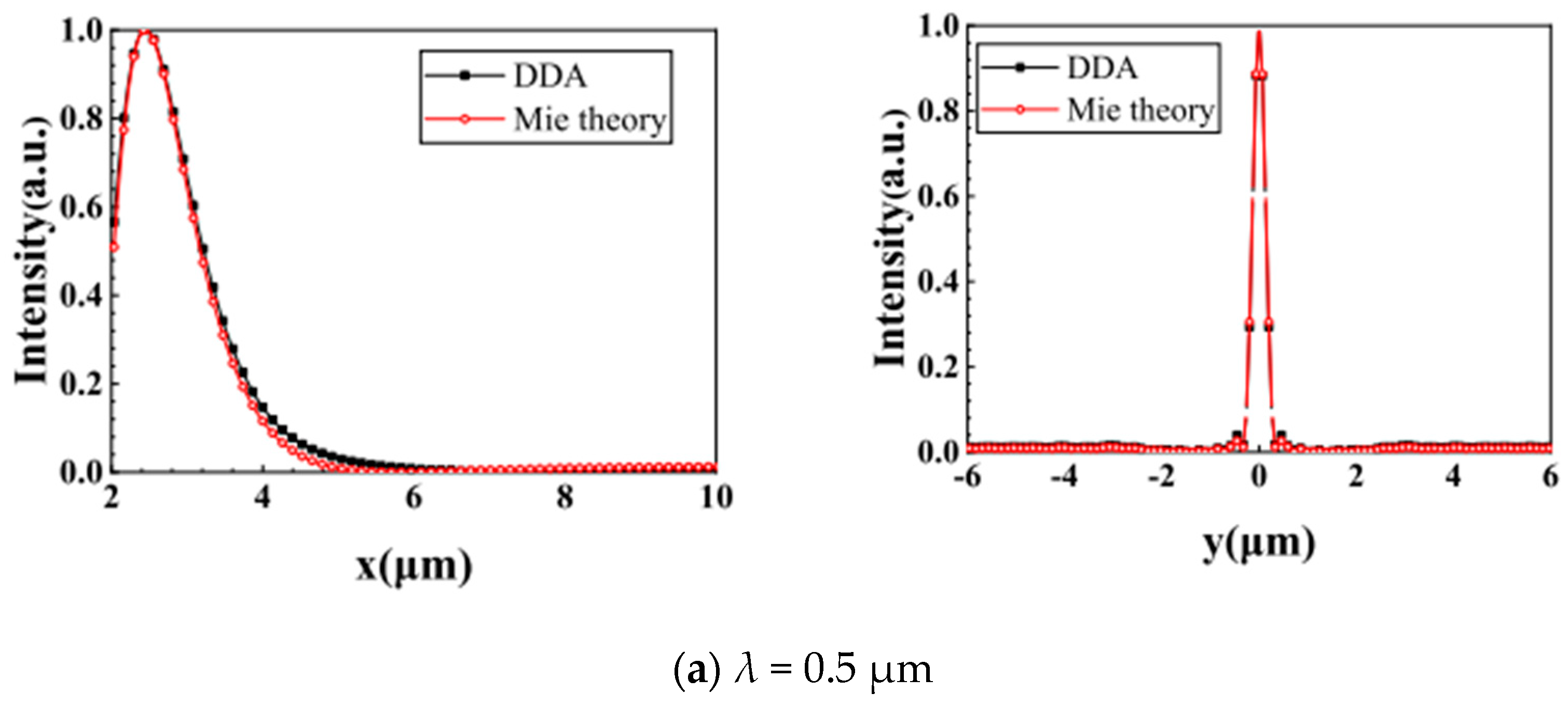
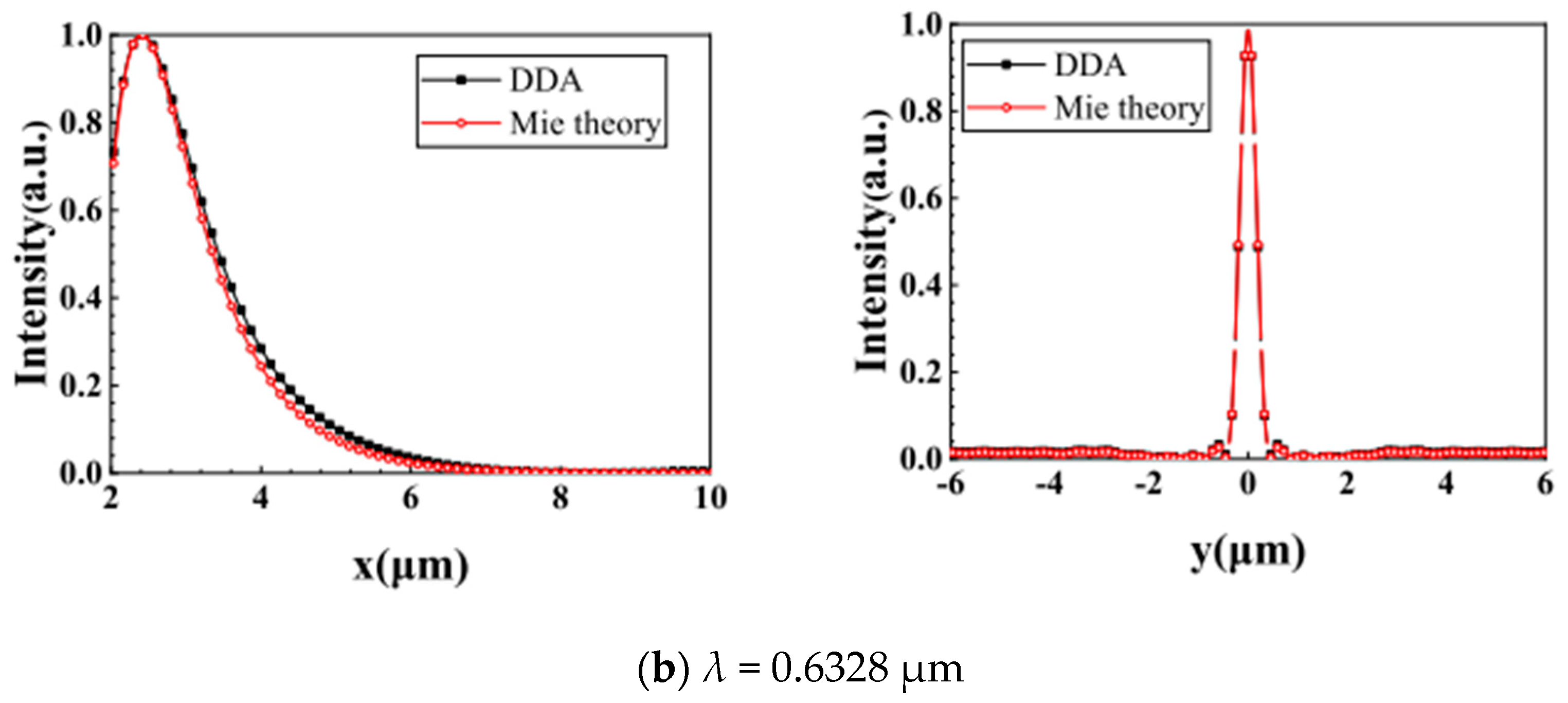
3.1. Numerical Validation
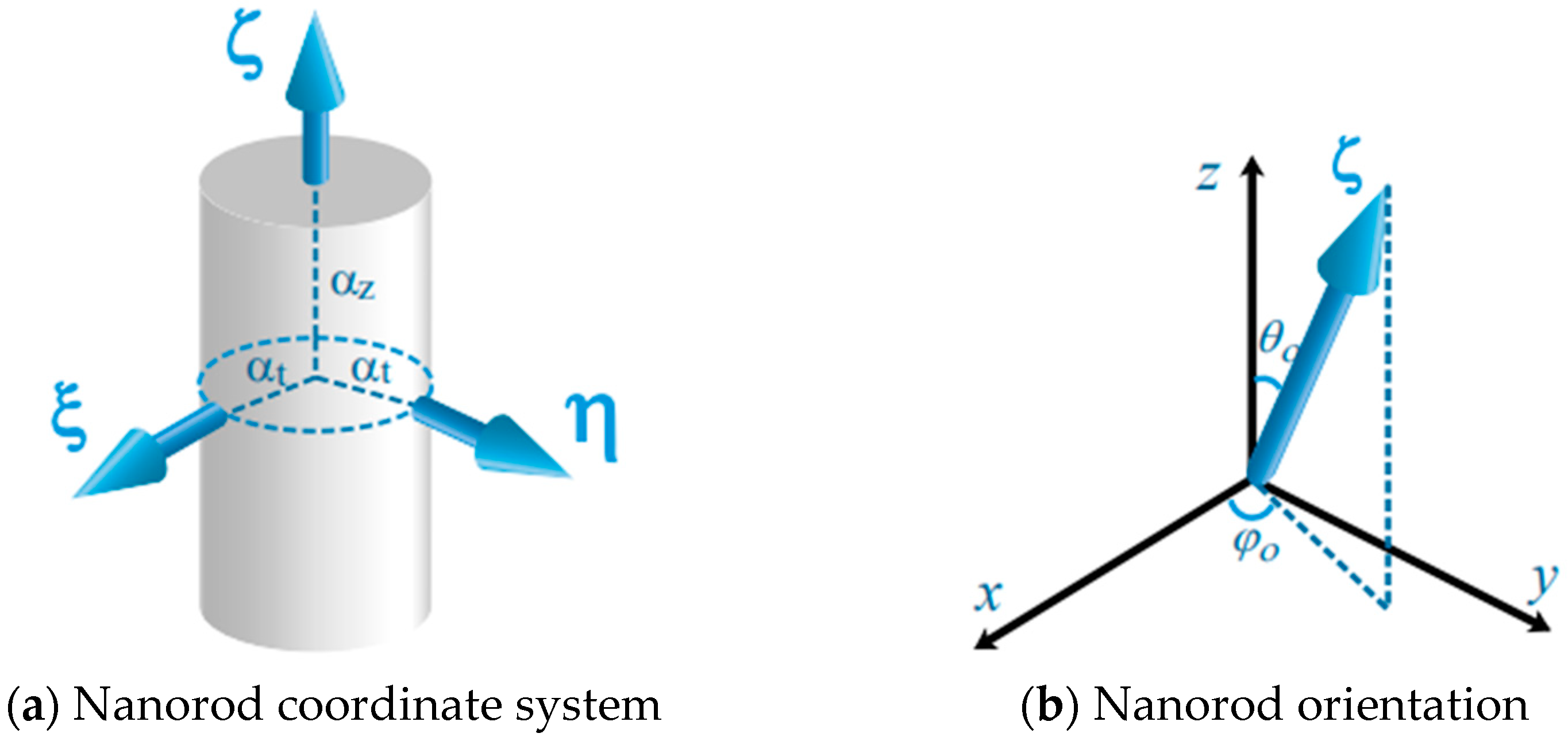
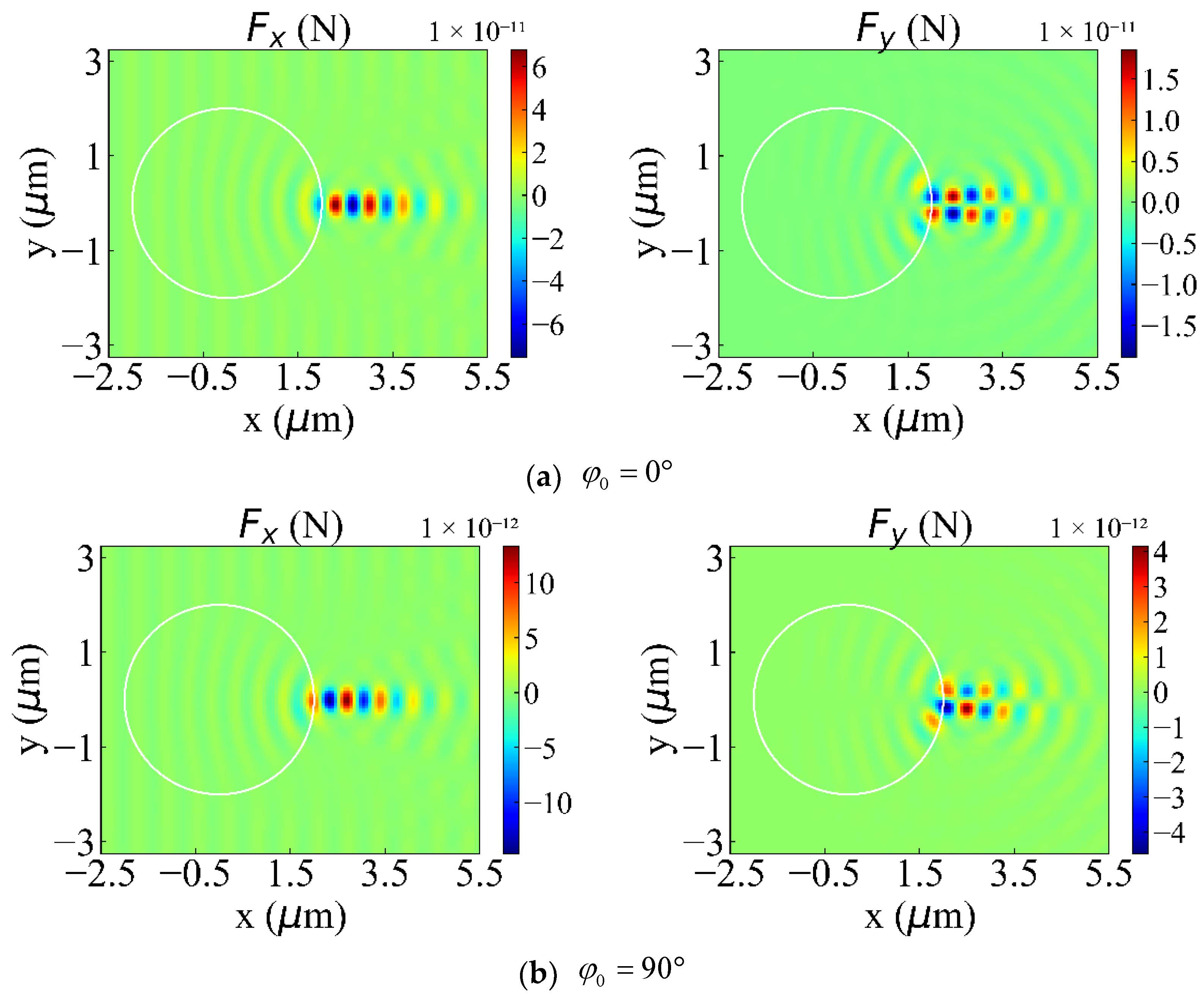
3.2. Orientation of Nanorods
3.2.1. Orientation of Nanorods
3.2.2. Orientation of Nanorods
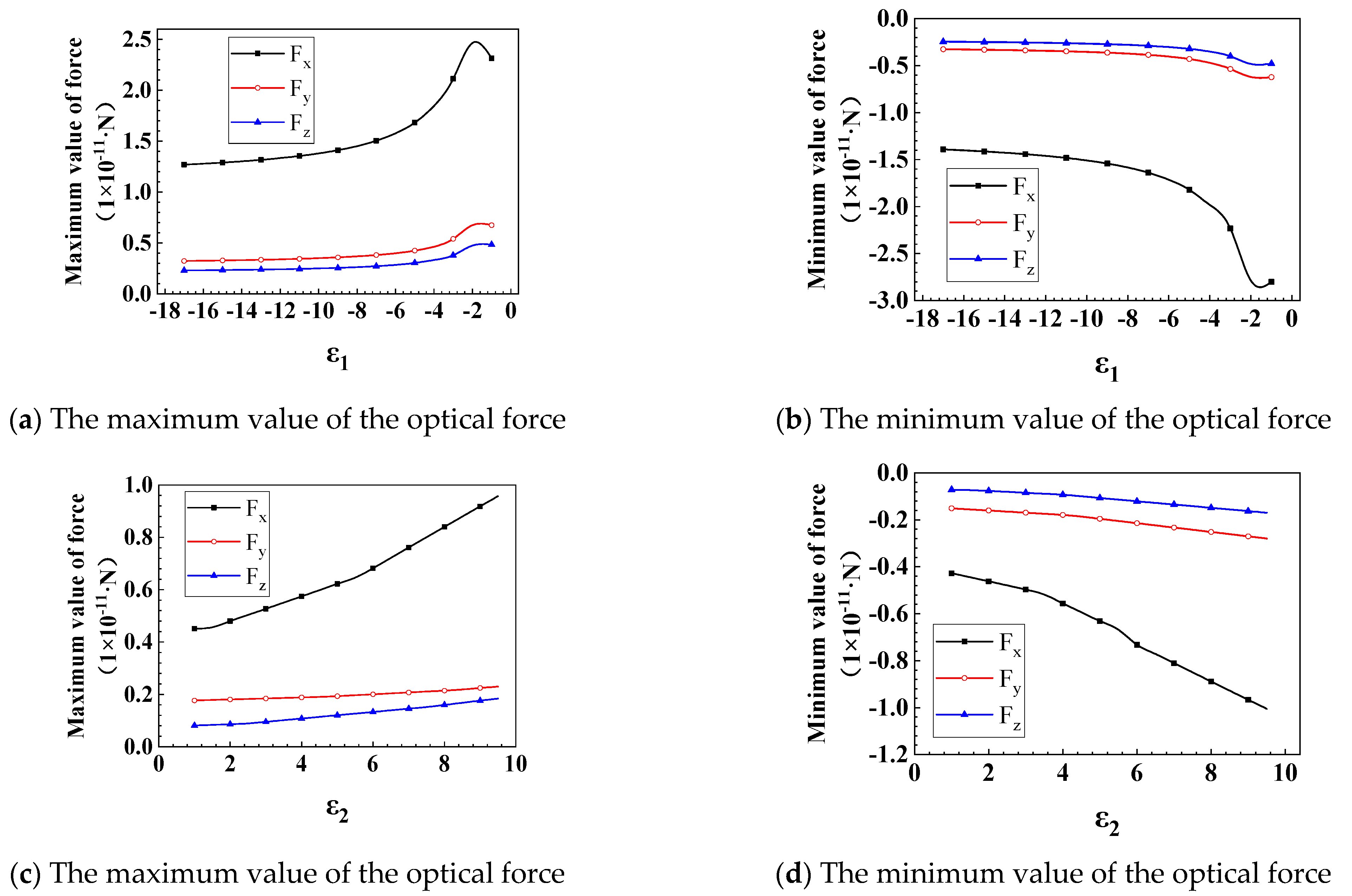
3.3. Dielectric Constant
4. Conclusions
Author Contributions
Funding
Data Availability Statement
Acknowledgments
Conflicts of Interest
Abbreviations
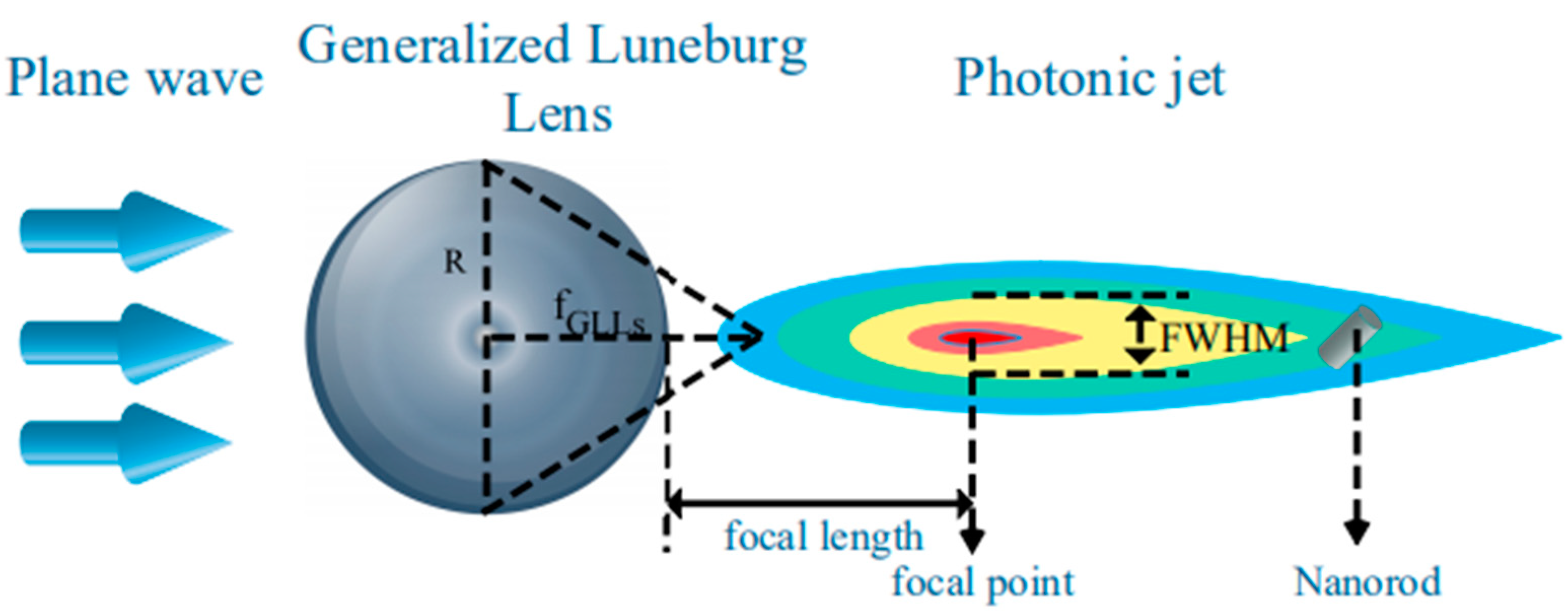
| PJ | Photonic jet |
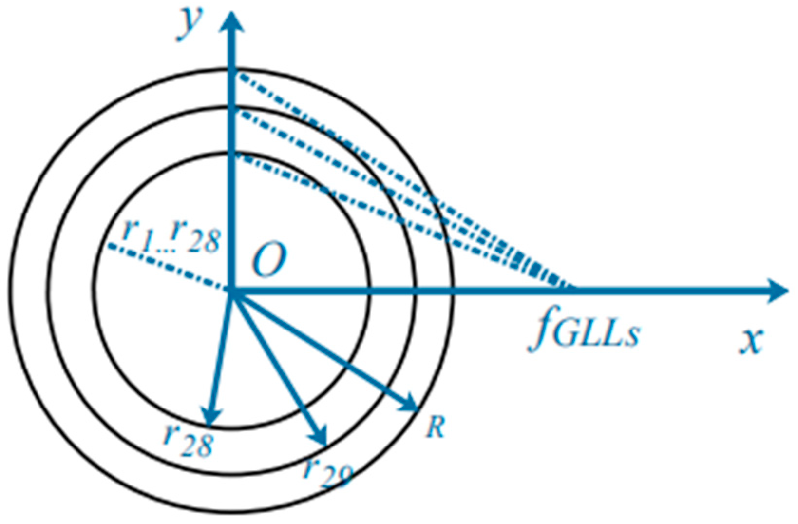
| GLLs | Generalized Luneburg Lens |
| DDA | Discrete Dipole Approximation |
| FWHM | Full Width at Half Maxima |
References
- Ashkin, A. Atomic-beam deflection by resonance-radiation pressure. Phys. Rev. Lett. 1970, 25, 1321–1324. [Google Scholar] [CrossRef]
- Ambardekar, A.A.; Li, Y.Q. Optical levitation and manipulation of stuck particles with pulsed optical tweezers. Opt. Lett. 2005, 301, 797–1799. [Google Scholar] [CrossRef] [PubMed]
- Oroszi, L.; Galajda, P.; Kirei, H.; Bottka, S.; Ormos, P. Direct measurement of torque in an optical trap and its application to double-strand dna. Phys. Rev. Lett. 2006, 97, 058301. [Google Scholar] [CrossRef]
- Ponelies, N.; Scheef, J.; Harim, A.; Leitz, G.; Greulich, K. Laser micromanipulators for biotechnology and genome research. J. Biotechnol. 1994, 35, 109–120. [Google Scholar] [CrossRef]
- Yao, J.; Li, L.; Li, P.; Yang, M. Quantum dots: From fluorescence to chemiluminescence, bioluminescence, electrochemiluminescence, and electrochemistry. Nanoscale 2017, 9, 13364–13383. [Google Scholar] [CrossRef] [PubMed]
- Fang, M.; Han, N.; Wang, F.; Yang, Z.X.; Yip, S.; Dong, G.; Hou, J.J.; Chueh, Y.; Ho, J.C. Cheminform abstract: Iii—v nanowires: Synthesis, property manipulations, and device applications. ChemInform 2015, 46. [Google Scholar] [CrossRef]
- Huang, X.; El-Sayed, I.H.; Qian, W.; El-Sayed, M.A. Cancer cell imaging and photothermal therapy in the near-infrared region by using gold nanorods. J. Am. Chem. Soc. 2006, 1282, 115–2120. [Google Scholar] [CrossRef]
- Maragò, O.M.; Jones, P.H.; Gucciardi, P.G.; Volpe, G.; Ferrari, A.C. Optical trapping and manipulation of nanostructures. Nat. Nanotechnol. 2013, 88, 07–819. [Google Scholar] [CrossRef] [Green Version]
- Pelton, M.; Liu, M.; Kim, H.Y.; Smith, G.; Guyot-Sionnest, P.; Scherer, N.F. Optical trapping and alignment of single gold nanorods by using plasmon resonances. Opt. Lett. 2006, 312, 2075–2077. [Google Scholar] [CrossRef]
- Selhuber-Unkel, C.; Zins, I.; Schubert, O.; Sönnichsen, C.; Oddershede, L.B. Quantitative optical trapping of single gold nanorods. Nano Lett. 2008, 82, 998–3003. [Google Scholar] [CrossRef]
- Tong, L.; Miljkovi´c, V.D.; Käll, M. Alignment, rotation, and spinning of single plasmonic nanoparticles and nanowires using polarization dependent optical forces. Nano Lett. 2010, 102, 68–273. [Google Scholar] [CrossRef]
- Ruijgrok, P.V.; Verhart, N.R.; Zijlstra, P.; Tchebotareva, A.L.; Orrit, M. Brownian fluctuations and heating of an optically aligned gold nanorod. Phys. Rev. Lett. 2011, 107, 037401. [Google Scholar] [CrossRef] [PubMed] [Green Version]
- Liaw, J.W.; Lo, W.J.; Kuo, M.K. Wavelength-dependent longitudinal polarizability of gold nanorod on optical torques. Opt. Express 2014, 221, 0858–10867. [Google Scholar] [CrossRef] [PubMed]
- Fick, J.; Leménager, G.; Thiriet, M.; Lallid, K.; Gacoin, T.; Valdivia-Valero, F.; Colas des Francs, G. Trapping of rare earth-doped nanorods with high aspect ratios using optical fiber-tip nano-tweezers. In Proceedings of the 2017 Conference on Lasers and Electro-Optics Europe European Quantum Electronics Conference, Munich, Germany, 25–29 June 2017. [Google Scholar]
- Huang, W.H.; Li, S.F.; Xu, H.T.; Xiang, Z.X.; Long, Y.B.; Deng, H.D. Tunable optical forces enhanced by plasmonic modes hybridization in optical trapping of gold nanorods with plasmonic nanocavity. Opt. Express 2018, 266, 202–6213. [Google Scholar] [CrossRef]
- Kong, S.C.; Sahakian, A.; Taflove, A.; Backman, V. Photonic nanojet-enabled optical data storage. Opt. Express 2008, 161, 3713–13719. [Google Scholar] [CrossRef] [PubMed]
- Chen, L.; Zhou, Y.; Li, Y.; Hong, M. Microsphere enhanced optical imaging and patterning: From physics to applications. Appl. Phys. Rev. 2019, 60, 21304. [Google Scholar] [CrossRef]
- Upputuri, P.K.; Wu, Z.; Gong, L.; Ong, C.K.; Wang, H. Super-resolution coherent anti-stokes raman scattering microscopy with photonic nanojets. Opt. Express 2014, 221, 2890–12899. [Google Scholar] [CrossRef]
- Minin, I.; Minin, O. Recent trends in optical manipulation inspired by mesoscale photonics and diffraction optics. J. Biomed. Photonics Eng. 2020, 6, 020301. [Google Scholar] [CrossRef]
- Minin, I.V.; Minin, O.V.; Liu, Y.Y.; Tuchin, V.V.; Liu, C.Y. Concept of photonic hook scalpel generated by shaped fiber tip with asymmetric radiation. J. Biophotonics 2021, 14, e202000342. [Google Scholar] [CrossRef]
- Ferrari, H.; Renner, G.; Luebrecht, S.; Love, G. High-frequency jet ventilation: Applications for endoscopy and surgery of the airway. South. Med. J. 1986, 799, 41–943. [Google Scholar] [CrossRef]
- Darafsheh, A.; Fardad, A.; Fried, N.M.; Antoszyk, A.N.; Ying, H.S.; Astratov, V.N. Contact focusing multimodal microprobes for ultraprecise laser tissue surgery. Opt. Express 2011, 193, 440–3448. [Google Scholar] [CrossRef]
- Mao, X.; Yang, Y.; Dai, H.; Luo, D.; Yao, B.; Yan, S. Tunable photonic nanojet formed by Generalized Luneburg Lens. Opt. Express 2015, 232, 6426–26433. [Google Scholar] [CrossRef]
- DeVoe, H. Optical properties of molecular aggregates. I. classical model of electronic absorption and refraction. J. Chem. Phys. 1964, 413, 93–400. [Google Scholar] [CrossRef]
- DeVoe, H. Optical properties of molecular aggregates. II. Classical theory of the refraction, absorption, and optical activity of solutions and crystals. J. Chem. Phys. 1965, 433, 199–3208. [Google Scholar] [CrossRef]
- Yon, J.; Liu, F.; Morán, J.; Fuentes, A. Impact of the primary particle polydispersity on the radiative properties of soot aggregates. Proc. Combust. Inst. 2019, 371, 151–1159. [Google Scholar] [CrossRef]
- Yurkin, M.A.; de Kanter, D.; Hoekstra, A.G. Accuracy of the discrete dipole approximation for simulation of optical properties of gold nanoparticles. J. Nanophotonics 2010, 4, 041585. [Google Scholar]
- Gordon, J.P. Radiation forces and momenta in dielectric media. Phys. Rev. A 1973, 8, 14–21. [Google Scholar] [CrossRef]
- Li, M.; Yan, S.; Yao, B.; Lei, M.; Yang, Y.; Min, J.; Dan, D. Trapping of rayleigh spheroidal particles by highly focused radially polarized beams. J. Opt. Soc. Am. B 2015, 324, 468–472. [Google Scholar] [CrossRef]
- Draine, B.T.; Flatau, P.J. Discrete-dipole approximation for scattering calculations. J. Opt. Soc. Am. A 1994, 111, 491–1499. [Google Scholar] [CrossRef]
- Yang, W.; Schatz, G.C.; Van Duyne, R.P. Discrete dipole approximation for calculating extinction and raman intensities for small particles with arbitrary shapes. J. Chem. Phys. 1995, 1038, 869–875. [Google Scholar] [CrossRef] [Green Version]
- Hoekstra, A.G.; Frijlink, M.; Waters, L.; Sloot, P. Radiation forces in the discrete-dipole approximation. JOSA A 2001, 181, 944–1953. [Google Scholar] [CrossRef] [Green Version]
- Amendola, V. Surface plasmon resonance of silver and gold nanoparticles in the proximity of graphene studied using the discrete dipole approximation method. Phys. Chem. Chem. Phys. 2016, 18, 2230–2241. [Google Scholar] [CrossRef] [PubMed]
- Jensen, T.; Kelly, L.; Lazarides, A.; Schatz, G. Electrodynamics of noble metal nanoparticles and nanoparticle clusters. J. Clust. Sci. 1999, 102, 95–317. [Google Scholar]
- Collinge, M.J.; Draine, B.T. Discrete-dipole approximation with polarizabilities that account for both finite wavelength and target geometry. JOSA A 2004, 212, 2023–2028. [Google Scholar] [CrossRef] [Green Version]
- Yurkin, M.A.; Maltsev, V.P.; Hoekstra, A.G. The discrete dipole approximation for simulation of light scattering by particles much larger than the wavelength. J. Quant. Spectrosc. Radiat. Transf. 2007, 106, 546–557. [Google Scholar] [CrossRef] [Green Version]
- Loke, V.L.; Mengüç, M.P.; Nieminen, T.A. Discrete-dipole approximation with surface interaction: Computational toolbox for matlab. J. Quant. Spectrosc. Radiat. Transf. 2011, 1121, 1711–1725. [Google Scholar] [CrossRef]
- Draine, B.T.; Goodman, J. Beyond Clausius-Mossotti: Wave Propagation on a Polarizable Point Lattice and the Discrete Dipole Approximation. Astrophys. J. 1993, 405, 685. [Google Scholar] [CrossRef]
- Wei, B.; Xu, Q.; Li, R.; Zhang, S.; Gong, S.; Sun, H.; Song, N. Optical torque on a rayleigh particle by photonic jet. J. Quant. Spectrosc. Radiat. Transf. 2021, 272, 107775. [Google Scholar] [CrossRef]
- Chaumet, P.C.; Rahmani, A. Efficient iterative solution of the discrete dipole approximation for magnetodielectric scatterers. Opt. Lett. 2009, 349, 917–919. [Google Scholar] [CrossRef] [PubMed]
- Yurkin, M.; Hoekstra, A. The discrete dipole approximation: An overview and recent developments. J. Quant. Spectrosc. Radiat. Transf. 2007, 1065, 558–589. [Google Scholar] [CrossRef] [Green Version]
- Spector, M.; Ang, A.S.; Minin, O.V.; Minin, I.V.; Karabchevsky, A. Photonic hook formation in near-infrared with Mxene Ti3C2 nanoparticles. Nanoscale Adv. 2020, 2, 5312–5318. [Google Scholar] [CrossRef]
- Li, M.; Yan, S.; Yao, B.; Liang, Y.; Han, G.; Zhang, P. Optical trapping force and torque on spheroidal rayleigh particles with arbitrary spatial orientations. J. Opt. Soc. Am. A 2016, 331, 341–1347. [Google Scholar] [CrossRef]
- Trojek, J.; Chvátal, L.; Zemánek, P. Optical alignment and confinement of an ellipsoidal nanorod in optical tweezers: A theoretical study. J. Opt. Soc. Am. A 2012, 291, 224–1236. [Google Scholar] [CrossRef]
- Mitri, F.G. Adjustable vector Airy light-sheet single optical tweezers: Negative radiation forces on a subwavelength spheroid and spin torque reversal. Eur. Phys. J. D 2018, 722, 1–14. [Google Scholar] [CrossRef]
- Schäfer, J.P. Implementierung und Anwendung Analytischer und Numerischer Verfahren zur Lösung der Maxwellgleichungen für die Untersuchung der Lichtausbreitung in Biologischem Gewebe. Ph.D. Thesis, Univerität Ulm, Ulm, Germany, 2011. [Google Scholar]
- Schäfer, J.; Lee, S.C.; Kienle, A. Calculation of the near fields for the scattering of electromagnetic waves by multiple infinite cylinders at perpendicular incidence. J. Quant. Spectrosc. Radiat. Transf. 2012, 1132, 2113–2123. [Google Scholar] [CrossRef]
- Bohren, C.F.; Huffman, D.R. Absorption and Scattering of Light by Small Particlesl; John Wiley & Sons: Hoboken, NJ, USA, 2008. [Google Scholar]
- Lee, S. Dependent scattering of an obliquely incident plane wave by a collection of parallel cylinders. J. Appl. Phys. 1990, 684, 952–4957. [Google Scholar] [CrossRef]
- Kerker, M. Electromagnetic scattering (book reviews: The scattering of light and other electromagnetic radiation). Science 1970, 167, 861. [Google Scholar]
- Dobler, C.P.; Rosoff, J. SPSS for Introductory Statistics: Use and Interpretation/SPSS for Intermediate Statistics: Use and Interpretation. Am. Stat. 2005, 59, 352. [Google Scholar]
- Minin, O.V.; Minin, I.V. Optical phenomena in mesoscale dielectric particles. Photonics 2021, 8, 591. [Google Scholar] [CrossRef]


Publisher’s Note: MDPI stays neutral with regard to jurisdictional claims in published maps and institutional affiliations. |
© 2022 by the authors. Licensee MDPI, Basel, Switzerland. This article is an open access article distributed under the terms and conditions of the Creative Commons Attribution (CC BY) license (https://creativecommons.org/licenses/by/4.0/).
Share and Cite
Wei, B.; Gong, S.; Li, R.; Minin, I.V.; Minin, O.V.; Lin, L. Optical Force on a Metal Nanorod Exerted by a Photonic Jet. Nanomaterials 2022, 12, 251. https://doi.org/10.3390/nano12020251
Wei B, Gong S, Li R, Minin IV, Minin OV, Lin L. Optical Force on a Metal Nanorod Exerted by a Photonic Jet. Nanomaterials. 2022; 12(2):251. https://doi.org/10.3390/nano12020251
Chicago/Turabian StyleWei, Bojian, Shuhong Gong, Renxian Li, Igor V. Minin, Oleg V. Minin, and Leke Lin. 2022. "Optical Force on a Metal Nanorod Exerted by a Photonic Jet" Nanomaterials 12, no. 2: 251. https://doi.org/10.3390/nano12020251
APA StyleWei, B., Gong, S., Li, R., Minin, I. V., Minin, O. V., & Lin, L. (2022). Optical Force on a Metal Nanorod Exerted by a Photonic Jet. Nanomaterials, 12(2), 251. https://doi.org/10.3390/nano12020251