A High-Order Hybrid Approach Integrating Neural Networks and Fast Poisson Solvers for Elliptic Interface Problems

Abstract

A new high-order hybrid method integrating neural networks and corrected finite differences is developed for solving elliptic equations with irregular interfaces and discontinuous solutions. Standard fourth-order finite difference discretization becomes invalid near such interfaces due to the discontinuities and requires corrections based on Cartesian derivative jumps. In traditional numerical methods, such as the augmented matched interface and boundary (AMIB) method, these derivative jumps can be reconstructed via additional approximations and are solved together with the unknown solution in an iterative procedure. Nontrivial developments have been carried out in the AMIB method in treating sharply curved interfaces, which, however, may not work for interfaces with geometric singularities. In this work, machine learning techniques are utilized to directly predict these Cartesian derivative jumps without involving the unknown solution. To this end, physics-informed neural networks (PINNs) are trained to satisfy the jump conditions for both closed and open interfaces with possible geometric singularities. The predicted Cartesian derivative jumps can then be integrated in the corrected finite differences. The resulting discrete Laplacian can be efficiently solved by fast Poisson solvers, such as fast Fourier transform (FFT) and geometric multigrid methods, over a rectangular domain with Dirichlet boundary conditions. This hybrid method is both easy to implement and efficient. Numerical experiments in two and three dimensions demonstrate that the method achieves fourth-order accuracy for the solution and its derivatives.

1. Introduction

This paper addresses a two-dimensional (2D) or three-dimensional (3D) elliptic interface problem for the Poisson equation with a smooth function $\lambda$:

$$\Delta u\left(\mathbf{x}\right)+\lambda \left(\mathbf{x}\right)u\left(\mathbf{x}\right)=f\left(\mathbf{x}\right),\mathbf{x}\in {\Omega }^{-}\cup {\Omega }^{+}.$$

(1)

It is subject to the Dirichlet boundary condition, given as follows:

$$u\left(\mathbf{x}\right)=u_b\left(\mathbf{x}\right),\mathbf{x}\in \partial \Omega .$$

(2)

The domain $\Omega$ is assumed to be rectangular and is partitioned into subdomains $\Omega ={\Omega }^{+}\cup {\Omega }^{-}$ by an interface $\Gamma$. We denote the solution in each subdomain by $u^{+}$ and $u^{-}$. Across the interface $\Gamma$, the solution exhibits jump discontinuities governed by the following jump conditions:

$$\left[\left[u\left(\mathbf{x}\right)\right]\right]=\gamma \left(\mathbf{x}\right),\left[\left[u_n\left(\mathbf{x}\right)\right]\right]=\rho \left(\mathbf{x}\right),\mathbf{x}\in \Gamma ,$$

(3)

where the notation $\left[\right[·\left]\right]$ denotes the difference between the values of a quantity as it approaches $\Gamma$ from ${\Omega }^{+}$ and ${\Omega }^{-}$ (i.e., the value from the ${\Omega }^{+}$ side minus the value from the ${\Omega }^{-}$ side). The term $u_n$ represents the normal derivative $\nabla u·\mathbf{n}$, where $\mathbf{n}$ is the unit normal vector pointing from ${\Omega }^{-}$ to ${\Omega }^{+}$. The source term is piecewise continuous with $\left[\left[f\left(\mathbf{x}\right)\right]\right]={\left[f^{+}\left(\mathbf{x}\right)\right]}_{\Gamma }-{\left[f^{-}\left(\mathbf{x}\right)\right]}_{\Gamma }\ne 0$.

Interface problems pose significant challenges for traditional numerical methods due to the loss of solution regularity across the interface. To address this issue and recover numerical accuracy near the interface, various methods have been developed by enforcing the jump conditions given in (3) and (4) into the numerical discretization. These approaches enable the design of accurate and robust numerical algorithms, including the coupling interface method [1], the piecewise-polynomial interface method [2], the kernel-free integral equation method [3], the finite volume method [4], and the immersed finite element method (IFEM) [5,6].

Over the past few decades, finite difference methods using Cartesian grids have been intensively studied for elliptic interface problems. Notable examples include the immersed interface method (IIM) [7,8,9], the ghost fluid method (GFM) [10], and the matched interface and boundary (MIB) method [11,12]. Building on the MIB methods, the augmented matched interface and boundary (AMIB) method has recently been developed for two- and three-dimensional elliptic interface problems [13,14,15]. In the AMIB method, finite difference discretizations near an irregular interface are corrected by Cartesian derivative jumps defined on the interface, which are reconstructed via additional approximations. Moreover, such jumps are treated as auxiliary variables in an augmented system, so that they can be solved together with the unknown solution in an iterative procedure. By using fast Poisson solvers including the fast Fourier transform [13,14] and multigrid method [15] to invert the discrete Laplacian operator, the AMIB method is highly efficient, achieving fourth-order accuracy for both the solution and its gradient. Nontrivial developments have been carried out in the AMIB method [14,16] in treating sharply curved interfaces. Nevertheless, the fourth-order AMIB method assumes the interface is $C^1$ continuous, so that it may not be applicable to $C^0$ continuous interfaces involving geometric singularities.

In recent years, the application of neural networks, both shallow and deep, to solve elliptic interface problems has gained significant attention in the scientific computing community. Unlike traditional grid-based methods, neural networks are inherently mesh-free, making them highly effective for handling complex interfaces and irregular domains. Prominent approaches like the Deep Ritz method [17] and physics-informed neural networks (PINNs) [18] have been widely used for solving partial differential equations (PDEs) with smooth solutions. Building on these foundations, various neural network models have been developed specifically for elliptic interface problems [19,20,21,22,23,24]. While many of these methods utilize deep network architectures, recent advances have demonstrated that shallow networks can also effectively address interface problems, such as the discontinuity capturing shallow neural network (DCSNN) [25] and the cusp-capturing PINNs [22]. Despite their promise, these mesh-free neural network approaches face ongoing challenges in ensuring stability and achieving robust convergence rates. To address these limitations, a hybrid method combining neural network-based machine learning with the traditional FFT Poisson solver was developed in [26]. This approach incorporates interface conditions into a learned function while using regular finite difference discretizations, achieving second-order accuracy and effectively handling complex geometries.

In this work, we propose a novel fourth-order hybrid method, referred to as the corrected hybrid method, for solving the Poisson interface problem (1)–(3). This method combines neural network learning with corrected finite difference schemes, integrating elements from the machine learning framework of the hybrid method [26] and the corrected finite difference discretization with high-order fast Poisson solvers from the AMIB method [14]. The corrected hybrid method retains the advantages of the hybrid method, such as its implementation simplicity and ability to handle complex interface geometries, while preserving the high-order accuracy of the AMIB method.

In the AMIB method, the standard fourth-order finite difference scheme for the Laplacian operator is corrected using Cartesian derivative jumps, which require additional approximation treatments. To simplify this process, the corrected hybrid method employs neural networks to predict these derivative jumps directly. This approach reduces implementation complexity while maintaining accuracy. Unlike the original hybrid method, which uses shallow neural networks to approximate solution components with second-order accuracy, the corrected hybrid method utilizes neural networks to predict high-order jump quantities. These predictions are incorporated into a corrected finite difference scheme, enabling fourth-order accuracy.

It is important to emphasize that the objective of the corrected hybrid method is not to replace traditional numerical methods such as the AMIB or IIM or to compete with them across all dimensions. Instead, the goal is to provide an alternative approach that is particularly advantageous for its high accuracy and ease of implementation when addressing Poisson interface problems with non-homogeneous jump conditions. By leveraging fast Poisson solvers and machine learning, the corrected hybrid method achieves both computational efficiency and high-order accuracy. Moreover, the use of the correct hybrid method for solving an open interface problem will also be explored.

The rest of the paper is organized as follows. In Section 2, a high-order hybrid method is proposed to solve the elliptic interface problems. The incorporation of FFT and multigrid solvers will be discussed in treating elliptic equations with constant coefficients and variable coefficients. Section 3 is dedicated to the numerical results to demonstrate the performance of the proposed algorithm in 2D and 3D. The generalization of the corrected hybrid method will be considered in Section 4, so that one can solve an open interface problem. Finally, this paper ends with a summary in Section 5.

2. Theory and Algorithm

To solve the Possion interface problem, we first define a small region ${\Omega }_{\Gamma }\subset \Omega$ that encloses the interface $\Gamma$. This region consists of all points within a certain distance d from $\Gamma$, where d is small. Here, the distance between a point $\mathbf{x}\in \Omega$ and $\Gamma$ is defined as $\parallel \mathbf{x}-{\mathbf{x}}_{\Gamma }{\parallel }_2$ where ${\mathbf{x}}_{\Gamma }\in \Gamma$ and the line passing these two points is perpendicular to $\Gamma$. We assume that $u^{+}$, $u^{-}$, $f^{+}$, and $f^{-}$ are smooth extensions of the solution u and the source term f to ${\Omega }_{\Gamma }$, ensuring they are valid throughout this region. These extensions satisfy the Poisson equations for $\mathbf{x}\in {\Omega }_{\Gamma }$:

$$\begin{array}{c}\hfill \Delta u^{+}\left(\mathbf{x}\right)+\lambda u^{+}\left(\mathbf{x}\right)=f^{+}\left(\mathbf{x}\right),\mathbf{x}\in {\Omega }_{\Gamma },\end{array}$$

(4)

$$\begin{array}{c}\hfill \Delta u^{-}\left(\mathbf{x}\right)+\lambda u^{-}\left(\mathbf{x}\right)=f^{-}\left(\mathbf{x}\right),\mathbf{x}\in {\Omega }_{\Gamma }.\end{array}$$

(5)

In the present study, $u^{+}$ and $u^{-}$ are assumed to be $C^6$ continuous in ${\Omega }_{\Gamma }$. In other words, the original solution u to the Poisson interface problem (1)–(3) is piecewise $C^6$ continuous. The same regularity requirement is also assumed in the fourth-order AMIB method [13,14,15,27], which is essentially required for achieving the fourth order of accuracy in solving second-order PDEs by using the corrected finite difference.

2.1. Neural Network Approximation for the Difference Function

We will not seek to solve $u^{+}\left(\mathbf{x}\right)$ and $u^{-}\left(\mathbf{x}\right)$ over ${\Omega }_{\Gamma }$. Instead, we will consider the difference function, defined as $D\left(\mathbf{x}\right)=u^{+}\left(\mathbf{x}\right)-u^{-}\left(\mathbf{x}\right)$. By subtracting Equation (5) from Equation (4) and using the jump conditions in Equation (3), we derive that $D\left(\mathbf{x}\right)$ satisfies the following conditions along the interface $\Gamma$:

$$\begin{array}{c}\hfill D\left(\mathbf{x}\right)=\gamma \left(\mathbf{x}\right),{\partial }_{n}D\left(\mathbf{x}\right)=\rho \left(\mathbf{x}\right),\Delta D\left(\mathbf{x}\right)+\lambda \left(\mathbf{x}\right)D\left(\mathbf{x}\right)=\left[\left[f\left(\mathbf{x}\right)\right]\right],\mathbf{x}\in \Gamma .\end{array}$$

(6)

Based on the regularity assumption for $u^{+}$ and $u^{-}$, $D\left(\mathbf{x}\right)$ is $C^6$ continuous over ${\Omega }_{\Gamma }$. According to the universal approximation theory, such a smooth function can be approximated by a shallow, fully connected neural network. We thus propose using a simple neural network with one hidden layer to approximate $D\left(\mathbf{x}\right)$. The network parameters are optimized using machine learning. Training data are collected at M points on the interface, ${\{\left({\mathbf{x}}_i^{\Gamma }\right)\in \Gamma \}}_{i=1}^M$, where the target values are $\gamma \left({\mathbf{x}}_i^{\Gamma }\right)$, $\rho \left({\mathbf{x}}_i^{\Gamma }\right)$, and $\left[\left[f\left({\mathbf{x}}_i^{\Gamma }\right)\right]\right]$. The proposed physics-informed neural network (PINN) minimizes the following mean squared error loss function:

$$\begin{array}{cc}\hfill \mathrm{Loss}\left(\mathbf{p}\right)=& {\displaystyle \frac{1}{M}}{\displaystyle \sum _{i=1}^M}[{\left(D(\left({\mathbf{x}}_i^{\Gamma }\right);\mathbf{p})-\gamma \left({\mathbf{x}}_i^{\Gamma }\right)\right)}^2+{\left({\partial }_{n}D(\left({\mathbf{x}}_i^{\Gamma }\right);\mathbf{p})-\rho \left({\mathbf{x}}_i^{\Gamma }\right)\right)}^2\hfill \\ \hfill & +{\left(\Delta D(\left({\mathbf{x}}_i^{\Gamma }\right);\mathbf{p})+\lambda \left({\mathbf{x}}_i^{\Gamma }\right)D(\left({\mathbf{x}}_i^{\Gamma }\right);\mathbf{p})-\left[\left[f\left({\mathbf{x}}_i^{\Gamma }\right)\right]\right]\right)}^2],\hfill \end{array}$$

(7)

where $\mathbf{p}$ denotes the trainable parameters (weights and biases) of the NN. The Levenberg–Marquardt (LM) method [28] is used to minimize this loss function.

Unlike the hybrid method presented in [26], which decomposes the solution $u\left(\mathbf{x}\right)$ into singular and regular components, the proposed corrected hybrid method directly solves for the solution $u\left(\mathbf{x}\right)$. This is achieved by incorporating the Cartesian derivative jumps across the interface, as predicted by the NN function $D\left(\mathbf{x}\right)$. These predicted jump quantities are then utilized within a corrected finite difference discretization, enabling the accurate computation of $u\left(\mathbf{x}\right)$ while satisfying the necessary boundary conditions.

2.2. Prediction of Cartesian Derivative Jumps

For the finite difference discretization, we assume a uniform mesh spacing h in a 2D rectangular domain $\Omega =[a,b]\times [c,d]$. The grid points are defined as follows:

$$\begin{array}{c}\hfill x_i=a+ih,y_j=c+jh,i=0,\dots ,n_x,j=0,\dots ,n_y.\end{array}$$

(8)

The standard fourth-order finite difference discretization becomes invalid near interfaces due to the presence of jump discontinuities. To address this issue, corrections based on Cartesian derivative jumps can be used. For any interface point $({\alpha }_x,{\alpha }_y)\in \Gamma$, the jump in the k-th derivative of u is defined as follows:

$$\left[{\displaystyle \frac{{\partial }^{k}u}{\partial x^k}}\right]{|}_{({\alpha }_x,{\alpha }_y)}=\underset{(x,{\alpha }_y)\to ({\alpha }_x^{+},{\alpha }_y)}{lim}{\displaystyle \frac{{\partial }^{k}u}{\partial x^k}}-\underset{(x,{\alpha }_y)\to ({\alpha }_x^{-},{\alpha }_y)}{lim}{\displaystyle \frac{{\partial }^{k}u}{\partial x^k}},$$

(9)

where $k=0,1,\dots ,4$. Here, $(x,{\alpha }_y)\to ({\alpha }_x^{+},{\alpha }_y)$ denotes the right-hand limit, and $(x,{\alpha }_y)\to ({\alpha }_x^{-},{\alpha }_y)$ denotes the left-hand limit. Note that the jump notation $[·]$ here is distinct from $\left[\right[·\left]\right]$, which is used in the jump conditions in Equation (3).

In the proposed corrected hybrid method, the approach to determine the Cartesian derivative jumps differs from the previous AMIB method [13,14,15,27]. For the case $k=0$, the zeroth-order Cartesian derivative jump is directly derived from the zeroth-order jump condition. For $k>1$, instead of relying on fictitious values generated by MIB schemes to reconstruct the Cartesian derivative jumps, the higher-order Cartesian derivative jumps are obtained with the aid of the difference function $D\left(\mathbf{x}\right)$ in this work.

Once the NN function $D\left(\mathbf{x}\right)$ is determined, the Cartesian derivative jump $\left[{\displaystyle \frac{{\partial }^{k}u}{\partial x^k}}\right]$ can be expressed in terms of the partial derivatives of the difference function ${\displaystyle \frac{{\partial }^{k}D}{\partial x^k}}$ at each interface point, scaled by a factor c:

$$\left[{\displaystyle \frac{{\partial }^{k}u}{\partial x^k}}\right]=c{\displaystyle \frac{{\partial }^{k}D}{\partial x^k}}.$$

(10)

The partial derivatives of the neural network approximation $D\left(\mathbf{x}\right)$ are efficiently computed using automatic differentiation [29]. The scaling factor c depends on the orientation of the interface crossing at the interface point. Specifically, $c=1$ if the grid line crosses the interface $\Gamma$ from ${\Omega }^{+}$ to ${\Omega }^{-}$, and $c=-1$ otherwise. This formulation applies equivalently to y- and z-grid lines.

By leveraging machine learning to predict these derivative jumps, the implementation is significantly simplified compared to the series of numerical approximations required by AMIB methods [13,14,15,27]. These predicted Cartesian derivative jumps are directly incorporated into the fourth-order corrected central differences, as detailed in the following subsection.

2.3. Fourth-Order Corrected Central Differences

We denote the standard fourth-order central difference operator for the second-order derivatives along the x-direction as follows:

$${\delta }_{xx}\left(x_i\right)=-{\displaystyle \frac{1}{12h^2}}u\left(x_{i-2}\right)+{\displaystyle \frac{4}{3h^2}}u\left(x_{i-1}\right)-{\displaystyle \frac{5}{2h^2}}u\left(x_i\right)+{\displaystyle \frac{4}{3h^2}}u\left(x_{i+1}\right)-{\displaystyle \frac{1}{12h^2}}u\left(x_{i+2}\right).$$

In the AMIB methods [13,14,15,27], such a standard central difference needs to be corrected near the interface. The corrected fourth-order central difference includes correction terms that incorporate the Cartesian derivative jumps at points where grid lines intersect the interface $\Gamma$. To simplify the discussion, we temporarily ignore the dependence of the solution on y and z, assuming $u=u\left(x\right)$. As in the AMIB methods [13,14,15,27], the solution u is assumed to be piecewise $C^6$ continuous, i.e., $C^6[x_i-h,\alpha )\cup C^6(\alpha ,x_{i+1}+h]$, with $x_i\le \alpha \le x_{i+1}$ and its derivatives extending continuously to the interface point $\alpha$.

When a jump discontinuity exists at the interface, the central difference operator must be adjusted locally. Using fourth-order corrected central differences, the Laplacian in the x-direction can be approximated as follows [13]:

$$\begin{array}{cc}\hfill u_{xx}\left(x_{i-1}\right)& \approx {\delta }_{xx}\left(x_{i-1}\right)+{\displaystyle \frac{1}{12h^2}}{\displaystyle \sum _{k=0}^K}{\displaystyle \frac{{\left(h^{+}\right)}^k}{k!}}\left[{\displaystyle \frac{{\partial }^{k}u}{\partial x^k}}\right],\hfill \end{array}$$

(11)

$$\begin{array}{cc}\hfill u_{xx}\left(x_i\right)& \approx {\delta }_{xx}\left(x_i\right)-{\displaystyle \frac{4}{3h^2}}{\displaystyle \sum _{k=0}^K}{\displaystyle \frac{{\left(h^{+}\right)}^k}{k!}}\left[{\displaystyle \frac{{\partial }^{k}u}{\partial x^k}}\right]+{\displaystyle \frac{1}{12h^2}}{\displaystyle \sum _{k=0}^K}{\displaystyle \frac{{(h+h^{+})}^k}{k!}}\left[{\displaystyle \frac{{\partial }^{k}u}{\partial x^k}}\right],\hfill \end{array}$$

(12)

$$\begin{array}{cc}\hfill u_{xx}\left(x_{i+1}\right)& \approx {\delta }_{xx}\left(x_{i+1}\right)+{\displaystyle \frac{4}{3h^2}}{\displaystyle \sum _{k=0}^K}{\displaystyle \frac{{\left(h^{-}\right)}^k}{k!}}\left[{\displaystyle \frac{{\partial }^{k}u}{\partial x^k}}\right]-{\displaystyle \frac{1}{12h^2}}{\displaystyle \sum _{k=0}^K}{\displaystyle \frac{{(h^{-}-h)}^k}{k!}}\left[{\displaystyle \frac{{\partial }^{k}u}{\partial x^k}}\right],\hfill \end{array}$$

(13)

$$\begin{array}{cc}\hfill u_{xx}\left(x_{i+2}\right)& \approx {\delta }_{xx}\left(x_{i+2}\right)-{\displaystyle \frac{1}{12h^2}}{\displaystyle \sum _{k=0}^K}{\displaystyle \frac{{\left(h^{-}\right)}^k}{k!}}\left[{\displaystyle \frac{{\partial }^{k}u}{\partial x^k}}\right],\hfill \end{array}$$

(14)

where $h^{-}=x_i-\alpha$, $h^{+}=x_{i+1}-\alpha$, and the Cartesian derivative jumps $\left[{\displaystyle \frac{{\partial }^{k}u}{\partial x^k}}\right]$ are provided by Equation (10). These corrections focus on the x-direction, with analogous formulations for the y and z directions. The correction terms are designed to vanish at regular points but are specifically applied near interfaces at irregular points. By combining corrected differences across all directions, the Laplacian operator is effectively approximated. For fourth-order accuracy, we set $K=4$, resulting in a third-order local truncation error, $O\left(h^3\right)$, at irregular points while maintaining a global fourth-order convergence rate. However, correcting fourth-order central differences along Cartesian directions near interfaces introduces challenges related to corners. These corner cases, which arise during the correction process, are rigorously addressed in Theorems 1–4 of [15].

2.4. Fast Poisson Solvers

We introduce a 1D column vector Q of size $5N_2\times 1$ to represent the Cartesian derivative jumps $\left[{\displaystyle \frac{{\partial }^{k}u}{\partial x^k}}\right]$ and $\left[{\displaystyle \frac{{\partial }^{k}u}{\partial y^k}}\right]$ at the $N_2$ intersection points between grid lines and the interface. The unknown function values at the $N_1$ interior grid points within the domain $\Omega$ are organized in a 1D column vector U of dimension $N_1\times 1$.

Let $U_{i,j}$ denote the discrete solution corresponding to the analytical solution $u(x_i,y_j)$ at $(x_i,y_j)$. Based on the fourth-order corrected difference analysis discussed in the previous subsection, the resulting discretized Poisson equation in matrix form is expressed as follows:

$$\begin{array}{cc}\hfill (L_h+{\lambda }_{i,j})U_{i,j}+C_{i,j}=f_{i,j},& \mathrm{for}1\le i\le n_x-1,1\le j\le n_y-1,\hfill \end{array}$$

(15)

where $C_{i,j}$ represents the correction term, and $L_h{U}_{i,j}$ denotes the standard fourth-order finite difference approximation to the Laplace operator.

The matrix form of the discretized system (15) can be written as $\widehat{A}U+BQ=F$, where $\widehat{A}=A+D$, with A representing an $N_1$-by-$N_1$ discrete Laplacian matrix and D being an $N_1$-by-$N_1$ diagonal matrix containing the entries ${\lambda }_{i,j}$. B is an $N_1$-by-$5N_2$ matrix containing coefficients from the correction terms, and F represents the known right-hand side after applying boundary conditions. Moving the known correction term $BQ$ to the right-hand side yields

$$\widehat{A}U=F-BQ.$$

(16)

The inversion of the matrix $\widehat{A}$ can be efficiently performed using fast Poisson solvers, such as the Fast Fourier Transform (FFT) method [13,14,27], geometric multigrid methods [15], or other fast techniques. By leveraging corrected central differences and Cartesian derivative jumps, these solvers ensure that solution discontinuities near the interface do not compromise accuracy or efficiency.

The fast Poisson solvers discussed in this work, with slight variations in the fourth-order finite difference schemes used for the Laplace operator and the discrete matrix $\widehat{A}$, have been employed in our previous studies [13,14,15,27]. These solvers are designed to handle the PDE (1) with different cases of the coefficient $\lambda$.

• Fast Fourier Transform (FFT):
  The FFT solver is applied for Poisson problems with a constant coefficient $\lambda$. In this case, the discrete matrix $\widehat{A}$ is constructed using a fourth-order central difference scheme. Following the approach outlined in [13,14,27], the matrix $\widehat{A}$ is efficiently inverted using the FFT algorithm. This method requires the solution to exhibit either an anti-symmetric property across the boundaries of the rectangular domain or periodic boundary conditions to ensure compatibility with the FFT framework.
• Geometric Multigrid Method:
  The geometric multigrid method is employed for Possion problems involving a variable coefficient $\lambda$. To maintain accuracy, a fourth-order geometric multigrid approach is applied to invert the matrix $\widehat{A}$. As described in [15], the standard fourth-order central difference scheme is utilized at interior grid points far from the boundaries, while fourth-order one-sided finite difference approximations are employed near boundary-adjacent points to ensure high-order accuracy near the domain boundaries.

Let us summarize the proposed fourth-order hybrid neural network and corrected finite difference method for solving the Poisson interface problem, as described in Algorithm 1.

Algorithm 1 Fourth-Order Hybrid Neural Network and Corrected Finite Difference Method

1: Step 1: Train the neural network function D by minimizing the loss function (7) using the Levenberg–Marquardt (LM) optimizer and compute the partial derivatives ${\displaystyle \frac{{\partial }^{n}D}{\partial x^n}}$ and ${\displaystyle \frac{{\partial }^{n}D}{\partial y^n}}$ at intersection points of grid lines with the interface $\Gamma$ using automatic differentiation. 2: Step 2: Calculate the Cartesian derivative jumps at each intersection point on $\Gamma$ using Equation (9) and store these values in a vector Q, then determine the coefficients of the correction terms in Equation (10) and store them in a matrix B. 3: Step 3: Apply a fast Poisson solver to solve the corrected finite difference equation, yielding the solution U.

2.5. Comparison Remarks

A comparison of the proposed corrected hybrid method with the existing high-order numerical methods for elliptic interface problems is in order.

The proposed fourth-order corrected hybrid method is designed to solve a simple Poisson interface problem (1)–(3), and is inapplicable to more general interface problems considered in the fourth-order AMIB method [13,14,15,27], in which the derivative jump condition involves discontinuous material coefficients. However, the corrected hybrid method offers notable advantages for Poisson interface problems and is potentially easier to implement. Due to the mesh-free nature of the neural network component, the proposed corrected hybrid method can handle complex interface geometries with minimal effort. Implementing machine learning for Cartesian derivative jump approximation only requires providing the interface description, such as its parametric form and normal vector. In contrast, the AMIB methods [14,15,16] require introducing fictitious values to construct Cartesian derivative jumps. A recent AMIB development allows for representing a fictitious value by function values away from the interface and other previously solved fictitious values [16], so that a more complex geometry can be handled. However, the fictitious value generation becomes very challenging when using coarse meshes or dealing with geometric singularities [16]. The proposed corrected hybrid method eliminates the need for fictitious value generation, making it more straightforward and robust for handling complicated interface geometries. It is important to note that the neural network function $D\left(x\right)$ is trained only once and can be evaluated at any interface location, allowing it to be applied across multiple grid resolutions, independent of discretization. Furthermore, the proposed method retains the advantageous features of the AMIB method, including the use of fast Poisson solvers and corrected finite difference schemes to ensure both efficiency and solution accuracy.

We note that for the present Poisson interface problem (1)–(3), the Cartesian derivative jumps can be calculated by the immersed interface method (IIM) [7,8,9]. In the context of handling interface conditions, the tangential jump $\left[\left[u_{\tau }\right]\right]$ can be computed based on the condition $\left[\right[u\left]\right]=\gamma \left(\mathbf{x}\right)$. Coupled with the normal jump $\left[\left[u_n\left(\mathbf{x}\right)\right]\right]=\rho \left(\mathbf{x}\right)$, this allows for the analytical derivation of first-order Cartesian derivative jumps, namely, $\left[u_x\right]$ and $\left[u_y\right]$. For second-order derivative jumps, such as $\left[u_{xx}\right]$ and $\left[u_{yy}\right]$, the IIM [30] provides a framework for computing these values. This approach relies on the second-order tangential and normal derivative jumps $\left[\left[u_{\tau \tau }\right]\right]$ and $\left[\left[u_{nn}\right]\right]$. However, the implementation of this method can be complex due to the involvement of curvature terms. In contrast, the high-order IIM formulation [31] facilitates the derivation of higher-order derivative jumps. Nevertheless, the proposed neural network-based method presents an alternative approach that is both more straightforward and efficient, offering a simpler means to approximate Cartesian derivative jumps, including higher-order derivatives.

3. Numerical Results

In this section, we analyze the accuracy of the proposed corrected hybrid method in solving two- and three-dimensional Poisson interface problems. For a comparison, we also examine the performance of the second-order hybrid method [26]. Additionally, we evaluate the ray-casting AMIB scheme introduced in [14,15], where Cartesian derivative jumps are constructed using fictitious values generated via the ray-casting MIB scheme. For both the AMIB method and the proposed corrected hybrid method, either the fourth-order FFT solver or the geometric multigrid is employed to invert the discrete matrix $\widehat{A}$ in solving the resulting linear Equation (16).

In each test, the neural network function $D\left(\mathbf{x}\right)$ is represented using a shallow network with a sigmoid activation function. This network employs only a single hidden layer, which simplifies the architecture and ensures efficiency by requiring the training of only a few hundred parameters across all numerical examples. A few hundred training points are randomly sampled along the interface to effectively capture its physical features. However, for more complex problems, particularly in three-dimensional cases or those involving complex geometric features, a larger number of training points may be necessary to maintain accuracy. The source code accompanying this manuscript is available on GitHub (visited on 22 March 2025): https://github.com/szhao-ua/fourth-order-hybrid-method.

The accuracy of approximating solution gradients or fluxes is explored through several numerical examples. The discrete gradient $\nabla u=(u_x,u_y)$ is computed using a fourth-order corrected central difference scheme. This method incorporates the predicted Cartesian derivative jumps provided by the neural network along with the computed solution to achieve high accuracy. For instance, the fourth-order central difference for the x component of the gradient, denoted as ${\delta }_x$, is given by

$${\delta }_x\left(x_i\right)={\displaystyle \frac{1}{12h}}u\left(x_{i-2}\right)-{\displaystyle \frac{2}{3h}}u\left(x_{i-1}\right)+{\displaystyle \frac{2}{3h}}u\left(x_{i+1}\right)-{\displaystyle \frac{1}{12h}}u\left(x_{i+2}\right).$$

The corrected gradients are then computed as follows:

$$\begin{array}{cc}\hfill u_x\left(x_{i-1}\right)\approx & {\delta }_x\left(x_{i-1}\right)+{\displaystyle \frac{1}{12h}}{\displaystyle \sum _{k=0}^K}{\displaystyle \frac{{\left(h^{+}\right)}^k}{k!}}\left[{\displaystyle \frac{{\partial }^{k}u}{\partial x^k}}\right],\hfill \end{array}$$

(17)

$$\begin{array}{cc}\hfill u_x\left(x_i\right)\approx & {\delta }_x\left(x_i\right)-{\displaystyle \frac{2}{3h}}{\displaystyle \sum _{k=0}^K}{\displaystyle \frac{{\left(h^{+}\right)}^k}{k!}}\left[{\displaystyle \frac{{\partial }^{k}u}{\partial x^k}}\right]+{\displaystyle \frac{1}{12h}}{\displaystyle \sum _{k=0}^K}{\displaystyle \frac{{(h+h^{+})}^k}{k!}}\left[{\displaystyle \frac{{\partial }^{k}u}{\partial x^k}}\right],\hfill \end{array}$$

(18)

$$\begin{array}{cc}\hfill u_x\left(x_{i+1}\right)\approx & {\delta }_x\left(x_{i+1}\right)-{\displaystyle \frac{2}{3h}}\left(x_{i+1}\right){\displaystyle \sum _{k=0}^K}{\displaystyle \frac{{\left(h^{-}\right)}^k}{k!}}\left[{\displaystyle \frac{{\partial }^{k}u}{\partial x^k}}\right]+{\displaystyle \frac{1}{12h}}{\displaystyle \sum _{k=0}^K}{\displaystyle \frac{{(h^{-}-h)}^k}{k!}}\left[{\displaystyle \frac{{\partial }^{k}u}{\partial x^k}}\right],\hfill \end{array}$$

(19)

$$\begin{array}{cc}\hfill u_x\left(x_{i+2}\right)\approx & {\delta }_x\left(x_{i+2}\right)+{\displaystyle \frac{1}{12h}}{\displaystyle \sum _{k=0}^K}{\displaystyle \frac{{\left(h^{-}\right)}^k}{k!}}\left[{\displaystyle \frac{{\partial }^{k}u}{\partial x^k}}\right],\hfill \end{array}$$

(20)

The correction of fourth-order central differences for the gradient in all corner cases is addressed in detail in Theorems 1–4 of [15].

For simplicity, the computational domain $\Omega$ is assumed to be either a square (2D) or a cubic domain (3D), uniformly partitioned into subintervals in each direction $(n=n_x=n_y=n_z)$. The accuracy and convergence of the numerical solutions are assessed for 2D problems by measuring errors in the maximum norm defined as follows:

$$L_{\infty }(u-u_h)=\underset{(x_i,y_j)\in {\Omega }^{-}\cup {\Omega }^{+}}{max}|u(x_i,y_j)-u_h(x_i,y_j)|,$$

where $u(x_i,y_j)$ and $u_h(x_i,y_j)$ are, respectively, the analytical and numerical solution. Similarly, error norms for the derivatives in the gradient can be defined using the same maximum norm. These definitions naturally extend to 3D problems.

The successive error, which measures the difference between solutions at two levels of grid refinement, is defined as

$$L_{\infty }(u_h-u_{h/2})=\underset{(x_i,y_j)\in {\Omega }^{-}\cup {\Omega }^{+}}{max}|u_h(x_i,y_j)-u_{h/2}(x_i,y_j)|,$$

where $u_h$ and $u_{h/2}$ are the numerical solutions on the coarse and finer grids, respectively.

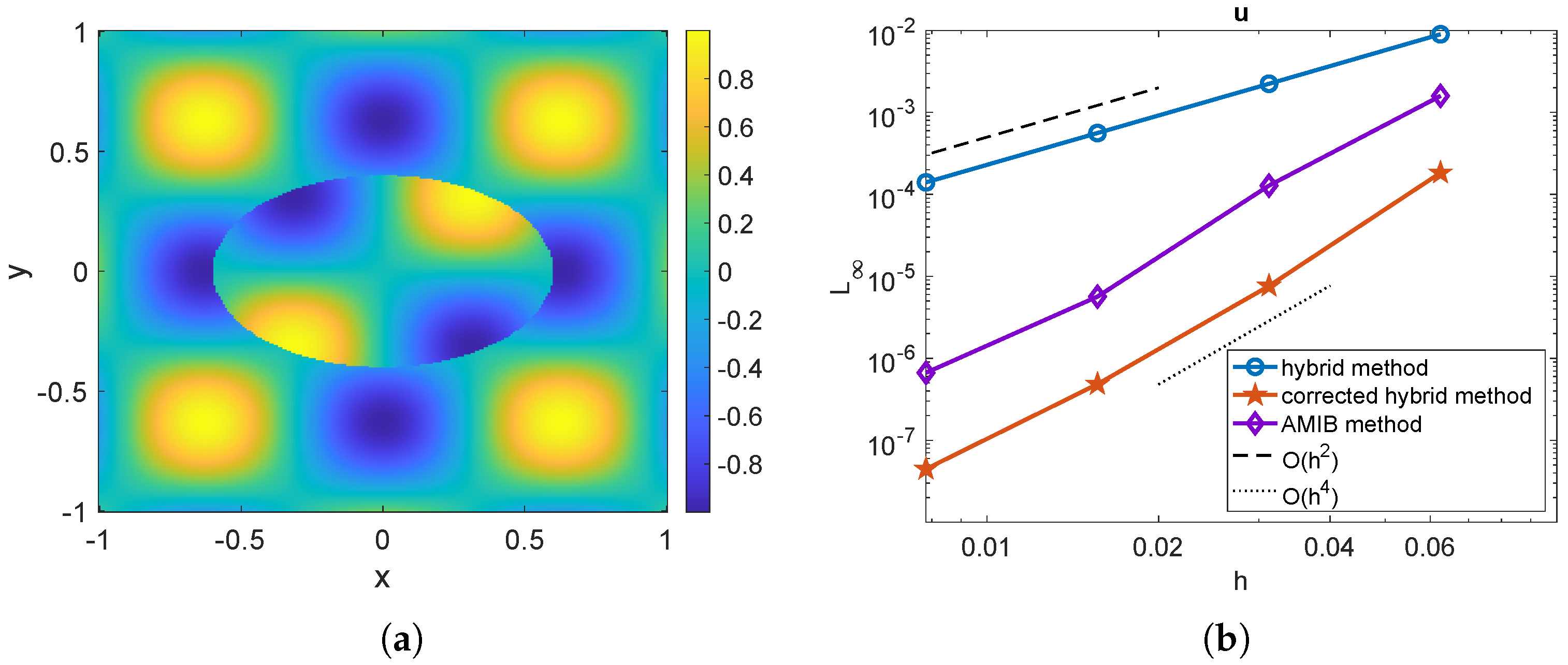
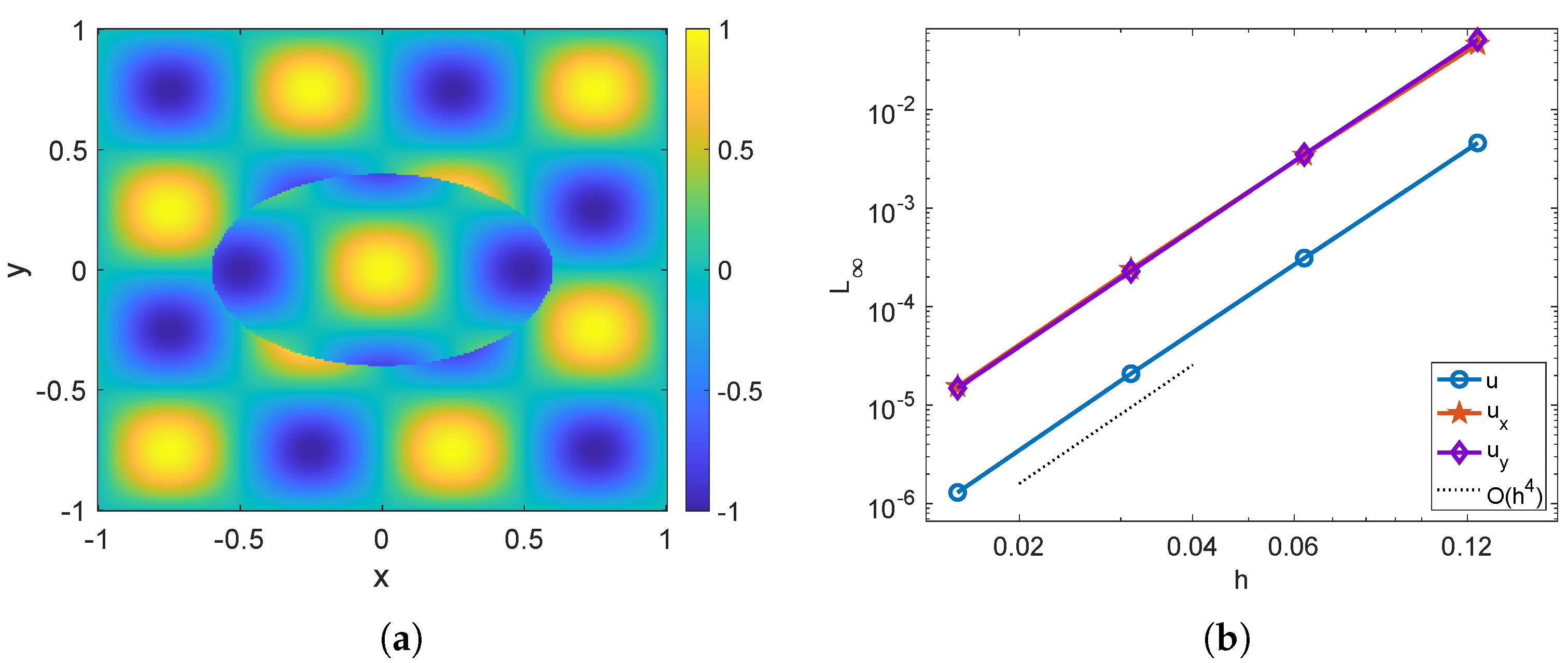
Example 1.

We begin by solving a two-dimensional Poisson interface problem and comparing the results of the proposed corrected hybrid method with those obtained using the AMIB method [15] and the original hybrid method [26]. The problem is defined on the square domain $\Omega ={[-1,1]}^2$, with the embedded interface represented by an ellipse:

$$\Gamma :{\left({\displaystyle \frac{x}{0.6}}\right)}^2+{\left({\displaystyle \frac{y}{0.4}}\right)}^2=1.$$

The exact solution is given by the following:

$$u(x,y)=\left\{\begin{array}{cc}sin\left(5x\right)sin\left(5y\right),\hfill & \mathit{if}(x,y)\in {\Omega }^{-},\hfill \\ cos\left(5x\right)cos\left(5y\right),\hfill & \mathit{if}(x,y)\in {\Omega }^{+},\hfill \end{array}\right.$$

from which the corresponding right-hand side $f(x,y)$, and jump conditions $\gamma (x,y)$ and $\rho (x,y)$ used in the loss function can be calculated accordingly. In this example, the geometric multigrid method is used to invert the matrix $\widehat{A}$ in both the proposed scheme and the AMIB scheme [15].

The same neural network setup is employed for both the present and the original hybrid methods. The network for $D\left(\mathbf{x}\right)$ is designed with 40 neurons in the hidden layer and trained using 200 randomly sampled training points on the interface $\Gamma$. The training process terminates when the stopping condition $\mathrm{Loss}\left(p\right)<{10}^{-12}$ is met or the maximum number of iterations (epoch = 1000) is reached.

The numerical solution for a mesh size of $h=1/128$ is displayed in Figure 1a. In Figure 1b, we present the mesh refinement study, showing the maximum norm error $L_{\infty }(u-u_h)$ as a function of the mesh size h. The results indicate that the original hybrid method (solid blue line with circular markers) achieves a second-order convergence rate, whereas both the proposed hybrid method (solid red line with pentagram markers) and the AMIB method (solid purple line with diamond markers) achieve a fourth-order convergence rate. 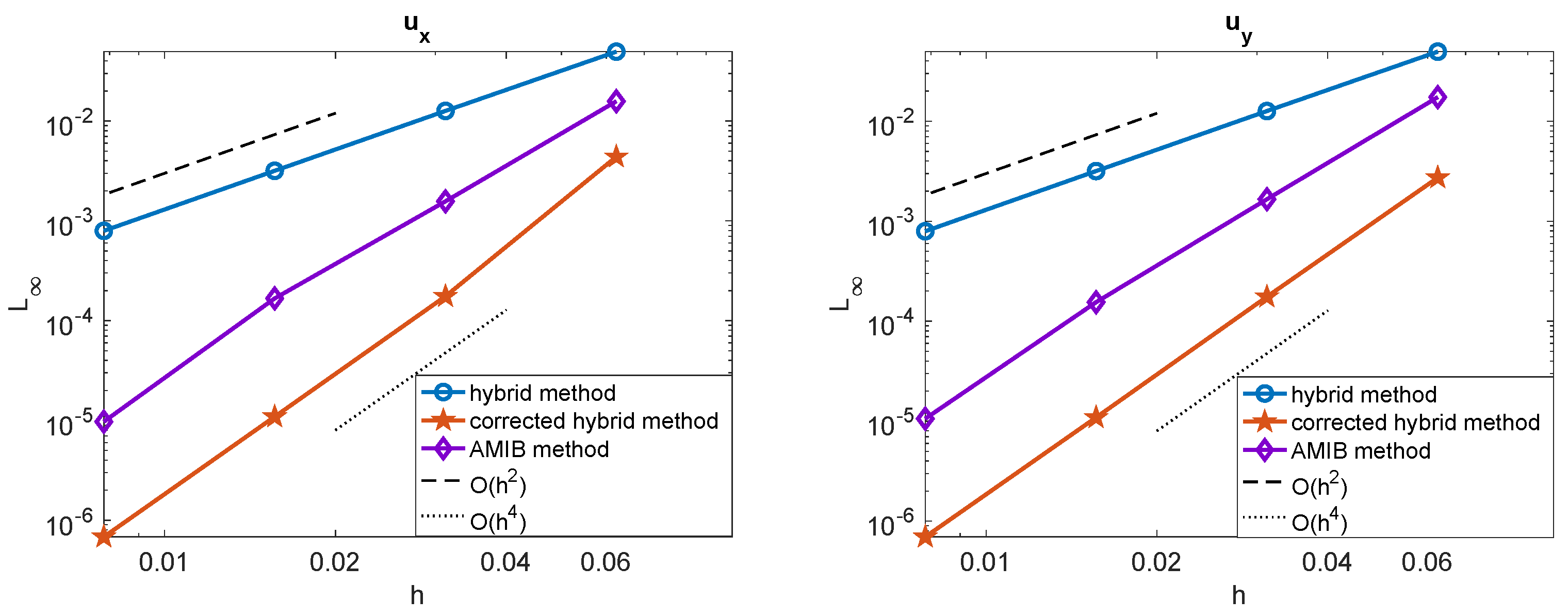In the present hybrid method, the computed solution is used to determine $\nabla u=(u_x,u_y)$ by applying the corrected finite difference scheme (17)–(20) with the predicted Cartesian derivative jumps. The gradients are also tested among these three methods, shown in Figure 2. The maximum errors of the gradients computed using the original hybrid method attain a second-order convergence rate, while the proposed hybrid method and the AMIB method achieve fourth-order convergence in the gradients.

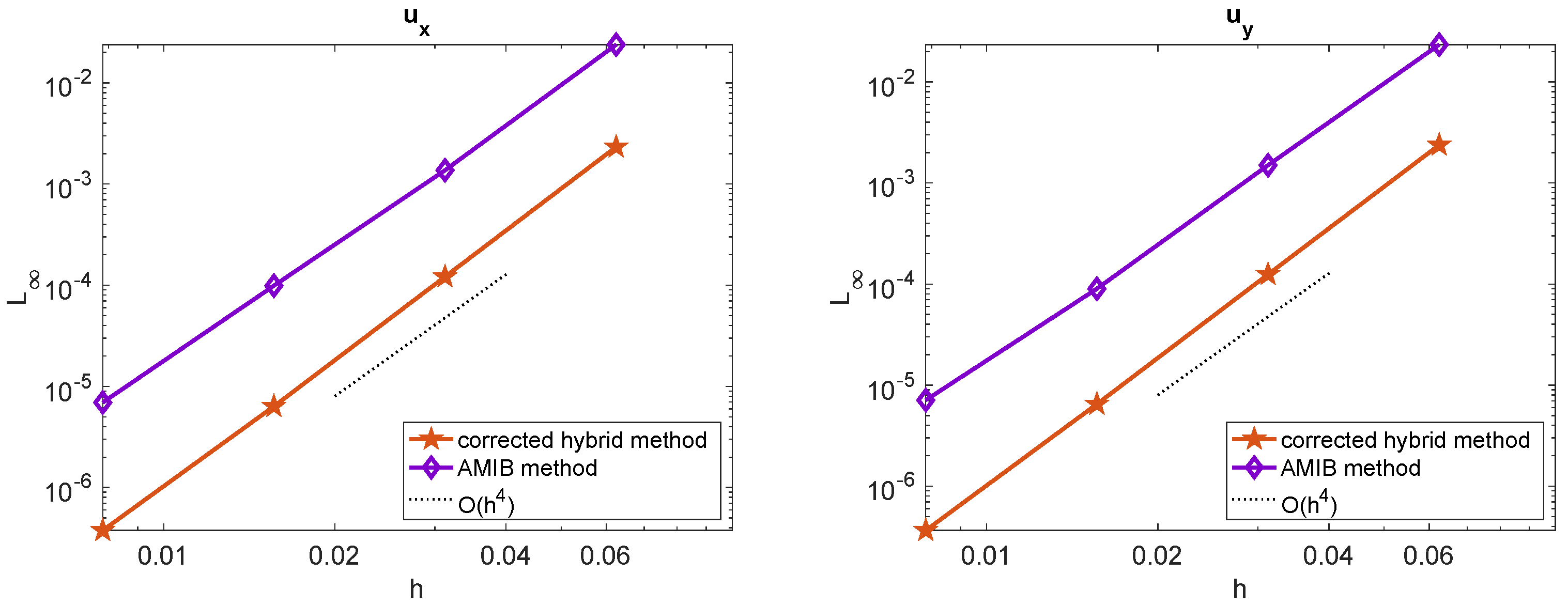
Next, we evaluate the performance of the proposed corrected method in solving the PDE (1) in the case of a variable coefficient $\lambda (x,y)$. The coefficient is set as $\lambda (x,y)=sin(x+y)+1$. The comparison of maximum errors for the solutions and gradients obtained using the AMIB method and the corrected hybrid method is presented in Figure 3 and Figure 4. The results demonstrate that both methods achieve a fourth-order convergence rate for both solutions and gradients.

The induced numerical error arises from two primary sources: the neural network approximation and the finite difference approximation. Although detailed results are not presented here, the final loss value achieved is approximately ${10}^{-12}$∼${10}^{-14}$. This corresponds to a predictive error, denoted as ${ϵ}^{\left(0\right)}$, of ${10}^{-6}$∼${10}^{-7}$ for the target function D. However, the predictive error ${ϵ}^{\left(k\right)}$ for higher-order (k-th) derivatives of D can grow exponentially with k, as seen in (10), which is used in the corrected finite difference schemes (11)–(14). To maintain fourth-order accuracy, the predictive error of the correction terms in (11)–(14), given by ${\displaystyle \frac{1}{h^2}}{ϵ}^{\left(0\right)}+{\displaystyle \frac{1}{h}}{ϵ}^{\left(1\right)}+{ϵ}^{\left(2\right)}+h{ϵ}^{\left(3\right)}+h^2{ϵ}^{\left(4\right)}$, must be smaller than the local truncation error $O\left(h^3\right)$. This indicates that the error is primarily dominated by the neural network approximation when the mesh size h is very small. To verify this observation, we conducted additional numerical tests with finer mesh widths. As expected, further refining the mesh did not lead to any significant reduction in the overall error, confirming that the neural network approximation is the limiting factor. A deeper or wider neural network architecture may achieve smaller predictive errors in the finer mesh.

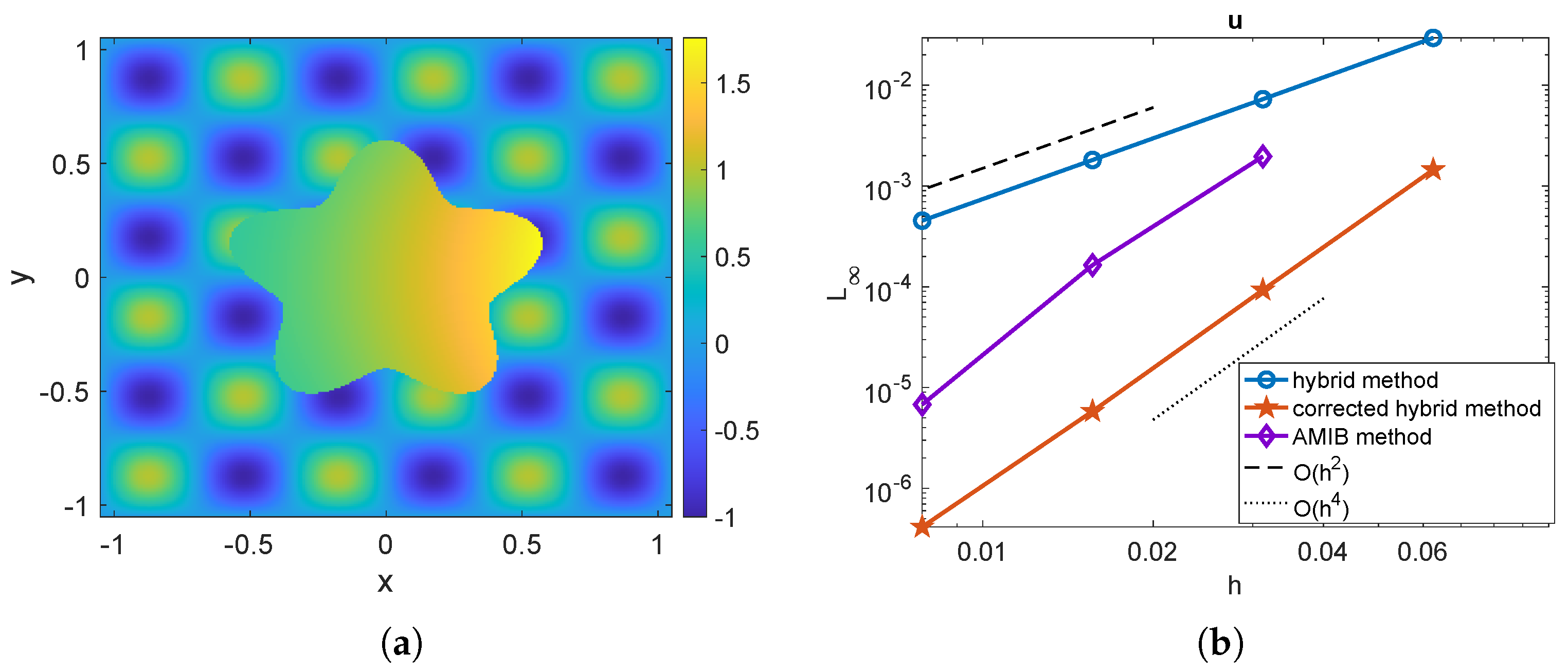
Example 2.

The second example concerns the Poisson equation and compares the performances of the three methods on a square domain $\Omega ={[-\pi /3,\pi /3]}^2$, with the embedded interface represented by a five-headed curve:

$$\Gamma :r\left(\theta \right)=0.5+0.1sin\left(\theta \right).$$

The exact solution is chosen as

$$u(x,y)=\left\{\begin{array}{cc}exp\left(x\right)cos\left(y\right),\hfill & \mathit{if}(x,y)\in {\Omega }^{-},\hfill \\ sin\left(kx\right)sin\left(ky\right),\hfill & \mathit{if}(x,y)\in {\Omega }^{+},\hfill \end{array}\right.$$

from which the corresponding jump information used in the loss function can be calculated accordingly. With $k=6$, a periodic boundary condition is imposed so that the FFT is employed to invert the matrix $\widehat{A}$ in both the proposed corrected hybrid scheme and the AMIB scheme [14]. The same neural network setup as in Example 1 is employed.

In Figure 5a, the numerical solution of the proposed scheme is shown for a mesh size of $h=1/128$, where the discontinuity is sharply captured across the interface. The mesh refinement results for the numerical solution and its gradient among the three methods are tested again and presented in Figure 5b and Figure 6, respectively. These results demonstrate that the original hybrid method achieves a second-order convergence rate for both the solution and the gradient. In contrast, both the proposed hybrid method and the AMIB method achieve a fourth-order convergence rate for both the solution and the gradient.

In Figure 5b and Figure 6, the AMIB method fails to produce numerical solutions and gradients on a coarse grid, whereas the corrected hybrid method remains robust. This discrepancy arises because, on coarse meshes, the AMIB method encounters difficulties in generating fictitious values and constructing accurate Cartesian derivative jumps. In contrast, the corrected hybrid method bypasses this challenge by leveraging its mesh-free neural network component, which ensures stability and accuracy even on coarser grids.

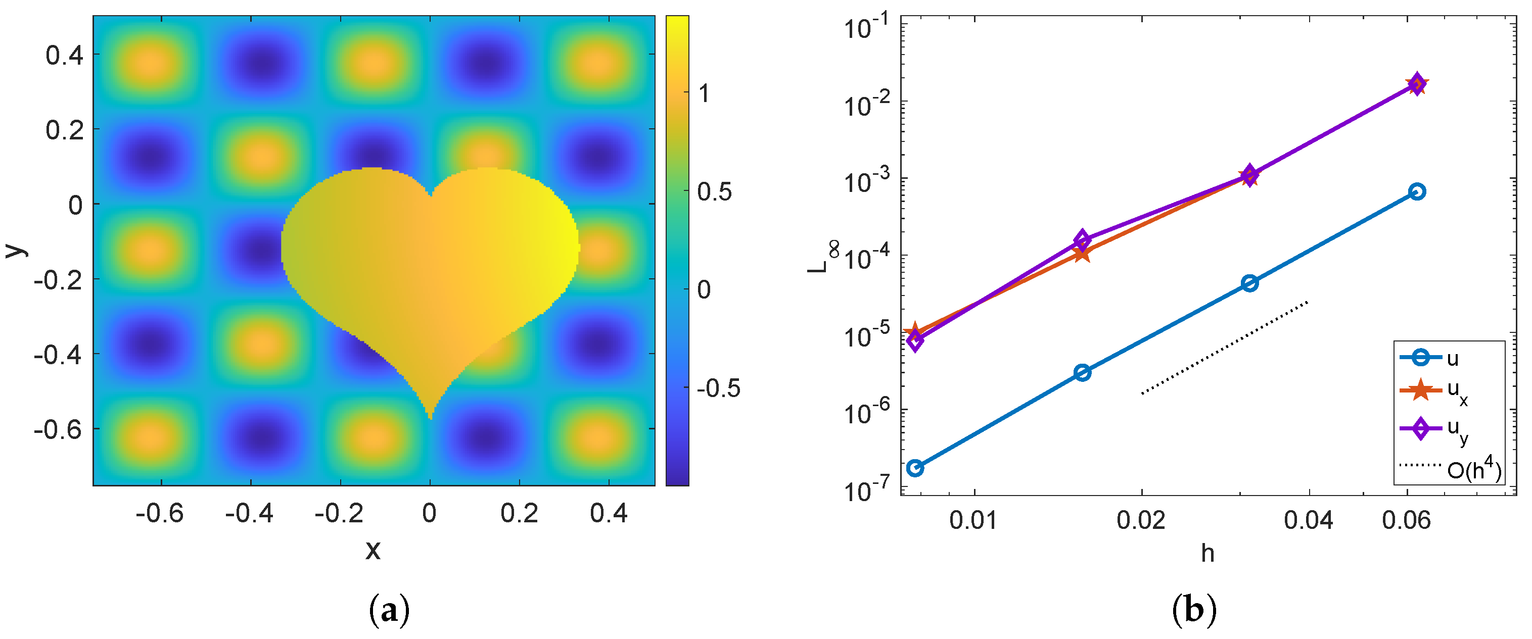
Example 3.

In this example, we consider a complex geometry with geometric singularities, which are beyond the capability of AMIB methods [13,14,15,16]. The problem is defined on the square domain $\Omega ={[-0.75,0.5]}^2$, with the embedded interface given by the heart-shaped curve:

$$\Gamma :r\left(\theta \right)=0.3-0.3sin\theta +0.3{\displaystyle \frac{sin\theta \sqrt{|cos\theta |}}{2sin\theta +2.8}}.$$

The heart-shaped interface features a singularity at the origin and the bottom tip, making it computationally challenging. The analytical solution and setup are identical to those in Example 2, except that $k=4$ is used. In Figure 7a, the numerical solution is shown for a mesh size of $h=5/1024$, demonstrating sharp discontinuity across the interface. Figure 7b presents the mesh refinement results for the numerical solution and its gradient. The proposed method exhibits fourth-order convergence for both the solution and the gradient.

Example 4.

To assess the reliability of the hybrid method, we consider a scenario where the exact solution is unavailable. The problem is defined on the square domain $\Omega ={[-1,1]}^2$, with the interface Γ embedded as an ellipse described by the following:

$$\Gamma :{\left({\displaystyle \frac{x}{0.6}}\right)}^2+{\left({\displaystyle \frac{y}{0.4}}\right)}^2=1.$$

The right-hand side function for the Poisson interface problem is chosen as follows:

$$f(x,y)=\left\{\begin{array}{cc}-2{\pi }^{2}cos\left(kx\right)cos\left(ky\right),\hfill & \mathit{if}(x,y)\in {\Omega }^{-},\hfill \\ -2{\pi }^{2}sin\left(kx\right)sin\left(ky\right),\hfill & \mathit{if}(x,y)\in {\Omega }^{+},\hfill \end{array}\right.$$

where $k=2\pi$. The Dirichlet boundary condition $u(x,y)=0$ is imposed along the boundary of Ω. With an unknown solution, the fourth-order geometric multigrid method is employed in this corrected hybrid method to invert $\widehat{A}$. At the interface Γ, the following jump conditions are prescribed:

$$\left[\right[u(x,y)\left]\right]=\gamma (x,y)=-cos\left(k\right(x+y\left)\right),$$

$$\left[\left[{\partial }_{n}u(x,y)\right]\right]=\rho (x,y)=ksin\left(k(x+y)\right)(n_1+n_2),$$

where $(n_1,n_2)$ represents the outward normal direction of Γ pointing from ${\Omega }^{-}$ to ${\Omega }^{+}$.

For this test, the neural network $D\left(\mathbf{x}\right)$ is configured with 150 neurons in a single hidden layer and is trained on 300 randomly sampled points along the interface $\Gamma$. Since the exact solution is unavailable, we evaluate the maximum error by computing the successive error $L^{\infty }(u_h-u_{h/2})$, where $u_h$ denotes the solution obtained with grid size h. In Figure 8a, we display the numerical solution u at the finest resolution $h=1/128$. In Figure 8b, the maximum norm errors for u and its gradient are presented. As anticipated, all quantities exhibit fourth-order convergence.

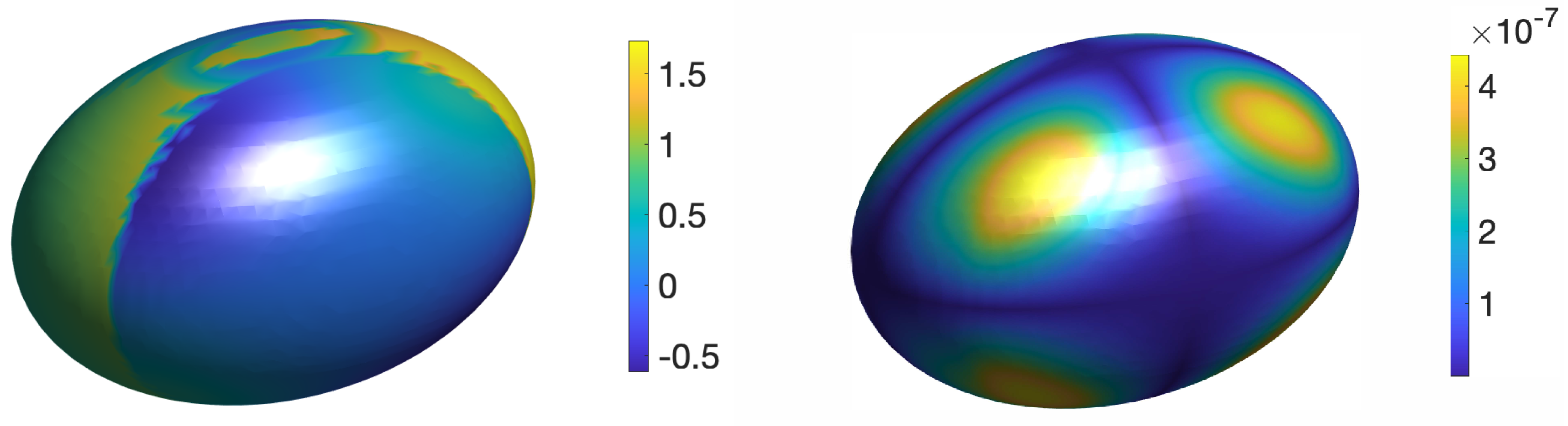
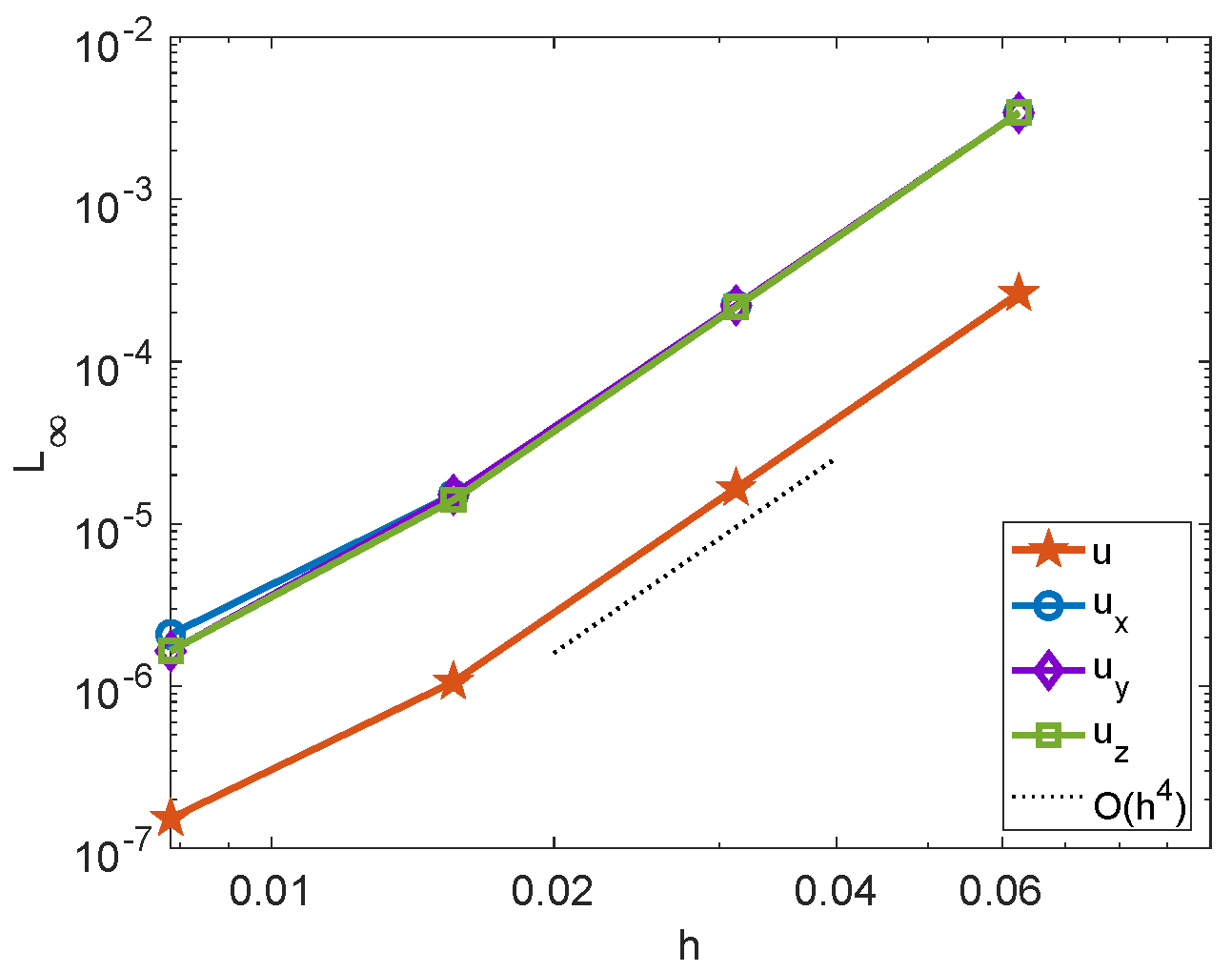
Example 5.

We consider a three-dimensional Poisson interface problem given in (1) with $\lambda =1$, where the interface is defined as an ellipsoid,

$$\Gamma :{\left({\displaystyle \frac{x}{0.5}}\right)}^2+{\left({\displaystyle \frac{y}{0.3}}\right)}^2+{\left({\displaystyle \frac{z}{0.2}}\right)}^2=1,$$

embedded in a cubic domain $\Omega ={\left[-\pi /3,\pi /3\right]}^3$. The exact solution is given by

$$u(x,y)=\left\{\begin{array}{cc}exp(x+y+z)\hfill & \mathit{if}(x,y,z)\in {\Omega }^{-},\hfill \\ sin\left(kx\right)sin\left(ky\right)sin\left(kz\right),\hfill & \mathit{if}(x,y,z)\in {\Omega }^{+},\hfill \end{array}\right.$$

So, the corresponding right-hand side $f(x,y,z)$, and the jump information $\gamma (x,y,z)$ and $\rho (x,y,z)$ are derived accordingly. We use the same shallow network structure as in the 2D examples: a single hidden layer containing 40 neurons. The network is trained using 200 points randomly sampled on the interface $\Gamma$ to learn the neural network function $D(x,y,z)$.

With $k=6$, the anti-symmetry property is satisfied at the boundary, allowing the use of the 3D FFT solver in both the corrected hybrid method and the 3D AMIB solver [14]. The numerical solutions and the maximum errors of the proposed corrected hybrid method are visualized in Figure 9, where the solutions and errors are mapped onto the ellipsoid surface $\Gamma$ from both the interior and exterior. 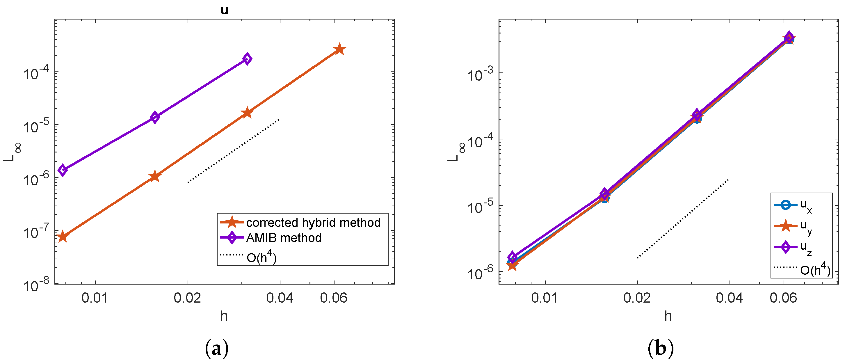Figure 10a presents the mesh refinement results, demonstrating that both the corrected hybrid method and the 3D AMIB solver [14] achieve fourth-order accuracy for the numerical solution. Notably, the proposed hybrid method exhibits higher accuracy than the AMIB solver. The corrected hybrid method utilizes a neural network to predict Cartesian derivative jumps in a straightforward, mesh-free manner, making it more robust and effective for handling complex interface geometries, especially in 3D. Similar to the 2D case, the AMIB solver fails for this 3D scenario with a mesh size of $h=1/16$, whereas the corrected hybrid method remains robust. Additionally, Figure 10b shows that the gradient of the proposed hybrid method also achieves fourth-order convergence.

Example 6.

We aim to solve a three-dimensional Poisson interface problem with geometric singularities. The interface is defined as an apple-shaped surface:

$$\Gamma :\rho =0.2375(1-cos\varphi ),$$

where $\rho =\sqrt{x^2+y^2+z^2}$ and $\varphi =arccos(z/\rho )$, embedded in a cubic domain $\Omega ={[-1,1]}^3$. The same neural network architecture and analytical solution with $k=2\pi$ as in Example 5 are employed.

The apple-shaped interface exhibits a singularity at the origin, which poses notable computational difficulties. The numerical solution and corresponding error of the corrected hybrid method on a mesh with $n=129$ are shown in Figure 11. The mesh refinement results for the numerical solution and its gradient are presented in Figure 12. These results demonstrate that the proposed corrected hybrid method achieves fourth-order convergence for both the solution and its gradient, even in the presence of geometric singularities.

4. Elliptic Interface Problem with Open Interface

To further explore the potential of the proposed corrected hybrid method, we will consider an elliptic interface problem with an open interface. Unlike a closed interface, an open interface extends to the boundary of the computational domain (see Figure 13a), introducing additional challenges for both neural network and numerical methods. In particular, open interface problems have not been studied before by using the original hybrid method [26] and the fourth-order AMIB method [13,14,15].

Since the proposed corrected hybrid method relies on a neural network trained to approximate the difference function $D\left(\mathbf{x}\right)$, we first further examine the mathematical definitions behind $D\left(\mathbf{x}\right)$ for interface problems. We first note that in Equations (4) and (5), we assume the governing equation can be extended over a small band ${\Omega }_{\Gamma }\subset \Omega$ containing all points within a certain distance d from $\Gamma$. Thus, the third jump condition for $D\left(\mathbf{x}\right)$ in Equation (6) is not only valid on the interface $\Gamma$. It can actually be extended to the subdomain ${\Omega }_{\Gamma }$ as follows:

$$\Delta D\left(\mathbf{x}\right)+\lambda \left(\mathbf{x}\right)D\left(\mathbf{x}\right)=f^{+}\left(\mathbf{x}\right)-f^{-}\left(\mathbf{x}\right),\mathbf{x}\in {\Omega }_{\Gamma }.$$

(21)

We note that in Equation (21), $f^{+}\left(\mathbf{x}\right)$ and $f^{-}\left(\mathbf{x}\right)$ are unavailable, respectively, in ${\Omega }^{-}\cap {\Omega }_{\Gamma }$ and ${\Omega }^{+}\cap {\Omega }_{\Gamma }$, according to the original elliptic interface (1)–(3). In the present study, we assume that the function expressions of $f^{+}\left(\mathbf{x}\right)$ and $f^{-}\left(\mathbf{x}\right)$ are given so that we can extend them to the other hand side of the interface $\Gamma$. When only nodal values of $f^{+}\left(\mathbf{x}\right)$ and $f^{-}\left(\mathbf{x}\right)$ are known, one can extrapolate these values to the other hand side of the interface $\Gamma$. Such approximations will be of high precision, because the band-width d is assumed to be small.

For a closed interface $\Gamma$, the three jump conditions given in Equation (6) over $\Gamma$ provide sufficient constraints for training $D\left(\mathbf{x}\right)$, since $D\left(\mathbf{x}\right)$ is implicitly influenced by neighboring points from all directions around the interface. Note that the interface information enforced in the loss function (7) is defined over a lower-dimensional set ($\Gamma$ is 1D in 2D problems). Such information becomes stand-alone only when $\Gamma$ is closed. However, in the case of an open interface, the three jump conditions no longer yield sufficient constraints in all directions near the interface because information is lost at the open ends.

For open interface problems, we propose using Equation (21) to replace the third jump condition in Equation (6) for predicting $D\left(\mathbf{x}\right)$. This provides more numerical stability for approximating higher-order derivatives of $D\left(\mathbf{x}\right)$. In fact, the present treatment aligns with the fundamental principle of finite difference stencils, where high-order derivative approximations achieve greater accuracy when computed over multiple points instead of a single location. To approximate $D\left(\mathbf{x}\right)$, training data are collected from $M_{\Gamma }$ interface points ${\{{\mathbf{x}}_i^{\Gamma }\in \Gamma \}}_{i=1}^{M_{\Gamma }}$ and $M_{{\Omega }_{\Gamma }}$ points in the small region ${\Omega }_{\Gamma }$, ${\{{\mathbf{x}}_i^{{\Omega }_{\Gamma }}\in {\Omega }_{\Gamma }\}}_{i=1}^{M_{{\Omega }_{\Gamma }}}$, where the target values are $\gamma \left({\mathbf{x}}_i^{\Gamma }\right)$, $\rho \left({\mathbf{x}}_i^{\Gamma }\right)$, and $f^{+}\left({\mathbf{x}}_i^{{\Omega }_{\Gamma }}\right)$, $f^{-}\left({\mathbf{x}}_i^{{\Omega }_{\Gamma }}\right)$. The neural network is trained by minimizing the following MSE loss function:

$$\begin{array}{cc}\hfill \mathrm{Loss}\left(\mathbf{p}\right)=& {\displaystyle \frac{1}{M_{\Gamma }}}{\displaystyle \sum _{i=1}^{M_{\Gamma }}}\left[{\left(D({\mathbf{x}}_i^{\Gamma };\mathbf{p})-\gamma \left({\mathbf{x}}_i^{\Gamma }\right)\right)}^2+{\left({\partial }_{n}D({\mathbf{x}}_i^{\Gamma };\mathbf{p})-\rho \left({\mathbf{x}}_i^{\Gamma }\right)\right)}^2\right]\hfill \\ \hfill & +{\displaystyle \frac{1}{M_{{\Omega }_{\Gamma }}}}{\displaystyle \sum _{i=1}^{M_{{\Omega }_{\Gamma }}}}\left[{\left(\Delta D({\mathbf{x}}_i^{{\Omega }_{\Gamma }};\mathbf{p})+\lambda \left({\mathbf{x}}_i^{{\Omega }_{\Gamma }}\right)D({\mathbf{x}}_i^{{\Omega }_{\Gamma }};\mathbf{p})-f^{+}\left({\mathbf{x}}_i^{{\Omega }_{\Gamma }}\right)+f^{-}\left({\mathbf{x}}_i^{{\Omega }_{\Gamma }}\right)\right)}^2\right],\hfill \end{array}$$

(22)

To minimize the loss function, we employ the LM method. Once the neural network function is obtained, the subsequent computational procedures remain the same as in the corrected hybrid method.

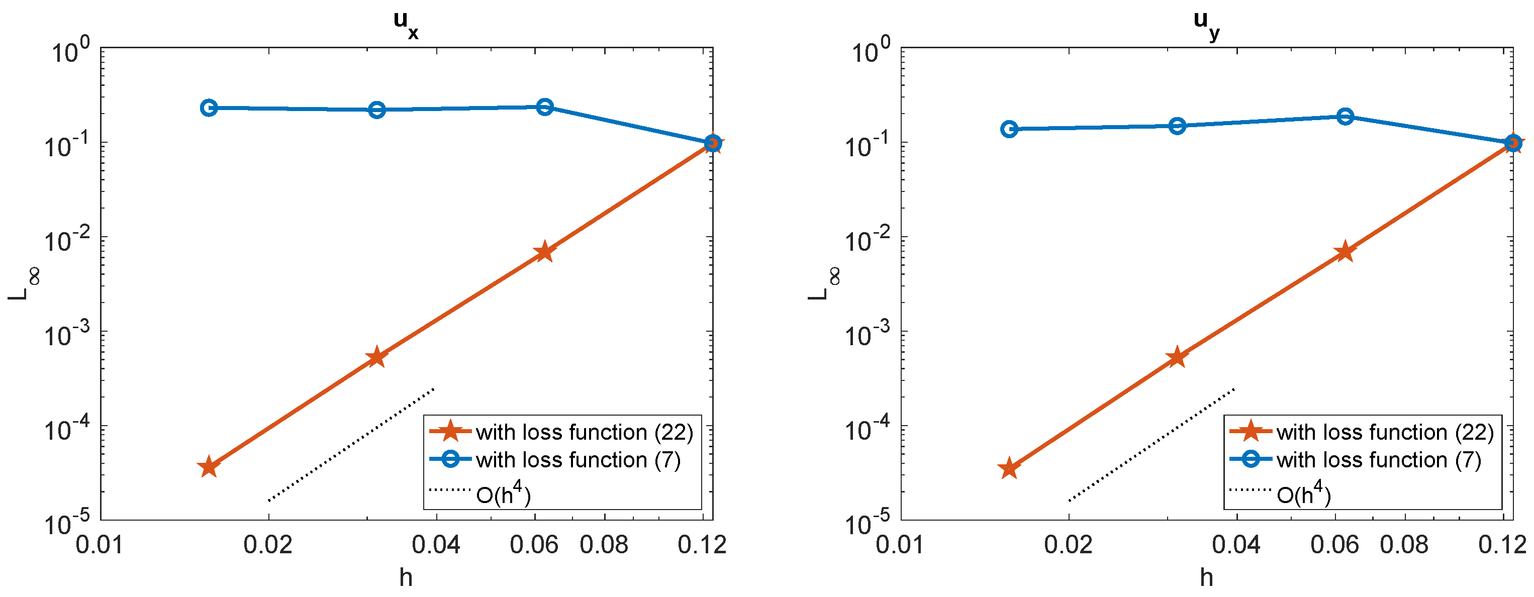
Example 7.

Consider an open interface given by the following equation:

$$\Gamma \left(x\right)=0.15tanh\left(exp\left({\displaystyle \frac{1}{1-x}}\right)exp\left({\displaystyle \frac{1}{1+x}}\right)\right),$$

defined on the domain $[-1,1]\times [-1,1]$ (see Figure 13a). The exact solution is the same as in Example 2 with $k=2\pi$.

For the neural network training, we employ a shallow network structure with $M_{\Gamma }=200$ points on the interface and $M_{{\Omega }_{\Gamma }}=200$ points in the small region ${\Omega }_{\Gamma }$. The solution of the corrected hybrid method, where the neural network is trained with the loss function in (22), is plotted in Figure 13a. The performance of the corrected hybrid method is evaluated by comparing the maximum errors of the solutions and gradients with the loss functions in (7) and (22). These comparisons are presented in Figure 13b and Figure 14, respectively. Using 40 neurons in the hidden layer, we observe that the loss function in (7) (with the third constraint applied directly on the interface) results in a lack of numerical stability of the high-order Cartesian derivative jumps, and consequently, the solution is inaccurate. In contrast, when the loss function in (22) is employed to train $D\left(\mathbf{x}\right)$, and the third constraint is applied in the small region ${\Omega }_{\Gamma }$, the solution and gradient achieve fourth-order convergence. This example demonstrates that the present corrected hybrid method is effective in solving elliptic interface problems with open interfaces.

However, extending the original hybrid method [26] to open interfaces might be challenging. Specifically, the neural network function is defined in ${\Omega }^{-}$, and since the open interface extends to the boundary of the domain, the information around the interface is incomplete. The missing information at the open ends makes it difficult to apply the jump conditions accurately, as there is no neighboring domain to provide the necessary context or constraints beyond the interface. Additionally, the region ${\Omega }_{\Gamma }$ around the open interface may not have a well-defined structure to enforce the smoothness conditions of the regular solution.

5. Conclusions

In this paper, we introduced a novel numerical method for solving elliptic interface problems, where the solution and its derivatives exhibit jump discontinuities across an interface. The proposed approach leverages machine learning to predict Cartesian derivative jumps by incorporating the given jump information into the loss function of a neural network. These predicted derivative jumps are then integrated into a corrected finite difference discretization of the Laplace operator. The resulting linear system is efficiently solved using a fast direct solver based on this corrected discretization.

We conducted numerical comparisons among the proposed corrected hybrid method, the original hybrid method [26], and the AMIB methods [14,15] for solving Poisson interface problems. Both the AMIB methods and the corrected hybrid method achieve fourth-order accuracy for both the solution and its derivatives, while the original hybrid method delivers a second-order convergence rate for both the solution and its derivatives. Notably, the corrected hybrid method demonstrated the highest accuracy among the three approaches. The corrected hybrid method excels in handling interfaces with geometric singularities, a capability not supported by AMIB methods, due to its mesh-free neural network framework. Additionally, it can be extended to open interfaces, where the interface extends to the boundary of the domain—an area where the original hybrid method might face challenges. Thus, the proposed method not only maintains high accuracy but also effectively addresses the challenges posed by geometric singularities and open interfaces.

However, as the mesh size h decreases, the overall error of the corrected hybrid method becomes primarily dominated by the neural network approximation. Further mesh refinement does not lead to a significant reduction in error, indicating that the neural network serves as the limiting factor in achieving higher-order accuracy.

Although the examples presented focus on cases with a single embedded interface, the method can be readily extended to accommodate multiple interfaces. Future work will explore extending this methodology to general elliptic interface problems with discontinuous material coefficients involved in the flux jump condition.