Ensemble of Filter-Based Rankers to Guide an Epsilon-Greedy Swarm Optimizer for High-Dimensional Feature Subset Selection

Abstract

The main purpose of feature subset selection is to remove irrelevant and redundant features from data, so that learning algorithms can be trained by a subset of relevant features. So far, many algorithms have been developed for the feature subset selection, and most of these algorithms suffer from two major problems in solving high-dimensional datasets: First, some of these algorithms search in a high-dimensional feature space without any domain knowledge about the feature importance. Second, most of these algorithms are originally designed for continuous optimization problems, but feature selection is a binary optimization problem. To overcome the mentioned weaknesses, we propose a novel hybrid filter-wrapper algorithm, called Ensemble of Filter-based Rankers to guide an Epsilon-greedy Swarm Optimizer (EFR-ESO), for solving high-dimensional feature subset selection. The Epsilon-greedy Swarm Optimizer (ESO) is a novel binary swarm intelligence algorithm introduced in this paper as a novel wrapper. In the proposed EFR-ESO, we extract the knowledge about the feature importance by the ensemble of filter-based rankers and then use this knowledge to weight the feature probabilities in the ESO. Experiments on 14 high-dimensional datasets indicate that the proposed algorithm has excellent performance in terms of both the error rate of the classification and minimizing the number of features.

1. Introduction

Results obtained by studies in machine learning show that feature subset selection can improve the performance of learning algorithms. The focus of feature subset selection is to remove irrelevant and redundant features from a certain dataset and choose a subset of features which give us the most information about the dataset [1]. From the machine learning point of view, if a system uses irrelevant features, it will use this information to predict the unseen data and, therefore, will guide the learning algorithm toward poor generalization. In addition to increasing the prediction accuracy of the learning algorithm, the feature subset selection has two other benefits: reducing the cost of collecting unnecessary data and reducing the learning and prediction time. However, dimensionality reduction by a feature subset selection algorithm, especially for high-dimensional datasets, is one of the most attractive branches of computer science and artificial intelligence.

Various algorithms have already been proposed to solve the feature subset selection problem. The simplest algorithm is to test all subsets by an exhaustive search algorithm, such as tree search algorithms, and select the best subset. Although this algorithm has a simple logic, directly evaluating all the feature subsets becomes a difficult optimization problem [2,3], because there are $2^d$ different feature subsets when we have a feature set with size d. Therefore, there are very few feature subset selection methods that use an exhaustive search in the feature space [1]. It is noteworthy that exhaustive search algorithms can only solve small- and medium-sized datasets and cannot be used for high-dimensional datasets because an exhaustive search in high-dimensional space is practically impossible. In this case, an approximate algorithm must be used which can remove redundant and irrelevant features with tractable and reasonable computations [2]. The approximate feature subset selection algorithms can be classified into three categories: filter methods, wrapper methods, and embedded methods [1]. Filter methods act as a preprocessing phase to rank all features wherein the top-ranked features are selected and used by a learning algorithm. In wrapper methods, the feature subset selection criterion is the performance of a learning algorithm, i.e., the learning algorithm is wrapped on a search algorithm which will find a subset that gives the highest learning algorithm performance. In other words, wrapper methods use the learning algorithm as a black box and the learning algorithm performance as the objective function to evaluate the feature subsets. Embedded methods try to use the advantages of both filter and wrapper methods.

Although the filter algorithms for feature subset selection are computationally efficient than wrapper algorithms, but they suffer severely from the “feature interaction problem”. We can generally define the feature interaction as a situation in which the optimization of a feature is affected by the values of other features. These interactions can be in two-way, three-way, or complex multi-way interactions among different features. For example, a feature that, individually, lacks meaningful relevance with the target, could dramatically increase the predictive accuracy of the learning algorithm if it is used in combination with other complementary features. In contrast, a feature that, individually, has good relevance to the target, may be a redundant feature in combination with other features. It should be noted that deleting or selecting these features, which is a highly probable task by the filter algorithms, can prevent us from finding the optimal feature subset. To avoid the feature interaction problem, we need to evaluate a subset of features as a whole with wrapper algorithms.

The wrapper methods were classified into two categories: sequential selection algorithms and meta-heuristic search algorithms [1,4]. The sequential selection algorithms start with an empty set (or a full set) and add features (or remove features) until the maximum value of objective function is obtained. Typical examples for sequential selection algorithms are sequential forward selection (SFS) [5] and sequential backward selection (SBS) [5]. Since sequential selection algorithms use the greedy approach, they suffer from the so-called “nesting effect” because a feature that is added or removed cannot be removed or added in later stages [6]. In the feature subset selection problem, the interaction between the features has a great impact on the accuracy of learning algorithm, so that a feature can be good on its own, but cannot produce good performance for learning algorithms in interaction with other features. Therefore, to find an optimal subset of features, the ability of removing and adding the features over time should be given [4]. In contrast to the sequential selection algorithms, meta-heuristic search algorithms evaluate different subsets to optimize the objective function [7]. Different subsets are generated either by searching around in a search space or by generating solutions to the optimization problem. The class of meta-heuristic search algorithms includes, but is not restricted to, Genetic Algorithms (GAs) [8], Particle Swarm Optimization (PSO) [9], Competitive Swarm Optimization (CSO) [10], Gravitational Search Algorithm (GSA) [11], and Ant Colony Optimization [12].

Although the accuracy of features obtained by the wrappers is better than the accuracy of the features obtained by the filters, in general, most of the wrappers do not perform well for high-dimensional feature subset selection [4]. There are two main reasons for this ineffectiveness. First, most algorithms perform the search in the high-dimensional feature space without any domain knowledge about the feature importance. Second, the most of existing algorithms are designed for continuous optimization problems, but the feature subset selection is essentially a binary optimization problem. Based on Xue et al. [4], one of the most important research fields for the feature subset selection problem is to propose new binary algorithms for solving the high-dimensional feature subset selection problem.

In this paper, we propose a novel hybrid filter-wrapper algorithm, called the Ensemble of Filter-based Rankers to guide an Epsilon-greedy Swarm Optimizer (EFR-ESO), for solving high-dimensional feature subset selection. Experiments on 14 high-dimensional datasets indicate that the proposed algorithm has a great performance both in terms of the error rate of the classification and in terms of minimizing the number of features. The two main contributions of this paper can be summarized as follows:

• A novel binary swarm intelligence algorithm, called the Epsilon-greedy Swarm Optimizer (ESO), is proposed as a new wrapper algorithm. In each iteration of the ESO, a particle is randomly selected, then the nearest-better neighbor of this particle in the swarm is found, and finally a new particle is created based on these particles using a new epsilon-greedy method. If the quality of new particle is better than the randomly-selected particle, the new particle is replaced in the swarm, otherwise the new particle is discarded.
• A novel hybrid filter-wrapper algorithm is proposed for solving high-dimensional feature subset selection, where the knowledge about the feature importance obtained by the ensemble of filter-based rankers is used to weight the feature probabilities in the ESO. The higher the feature importance, the more likely it is to be chosen in the next generation. In the best of our knowledge, no empirical research has been conducted on the using feature importance obtained by the ensemble of filter-based rankers to weight the feature probabilities in the wrapper algorithms.

The structure of this paper is organized as follows. In Section 2, the literature review of the paper is presented. In Section 3, the proposed EFR-ESO algorithm for the high-dimensional feature subset selection is introduced. Section 4 presents the theoretical global convergence analysis of EFR-ESO. Section 5 contains the experimental results of the paper, in which the numerical performance of the proposed algorithm for high-dimensional feature subset selection is evaluated and its results are compared with results of other feature subset selection algorithms. Finally, in Section 6 the conclusion and future work are given.

2. Literature Review

Research on meta-heuristic algorithms for feature subset selection began around the 1990s. However, these methods did not come to fame until around 2007, when the size of datasets became relatively large. In the best of our knowledge, Genetic Algorithms (GAs) are the first meta-heuristic widely used for feature subset selection. The results of the first research in the field of feature subset selection by GA was published in 1989 [13]. After that, many studies were done to improve the GA for feature subset selection. For example, Li et al. [14] suggested a GA with multiple populations for feature subset selection in which every two-neighbor population exchanged two solutions to share their obtained knowledge. In [15] a hybrid genetic algorithm (HGA) is proposed for feature subset selection, where the GA is combined with a local search.

Particle Swarm Optimization (PSO) is another meta-heuristic widely used for feature subset selection. Both continuous PSO and binary PSO have been used for solving this problem [4]. When using the continuous PSO for feature subset selection, a threshold λ is applied to specify the selection statues of a feature. If the feature value of a particle is larger than λ, the corresponding feature is selected. Otherwise, if the feature value of a particle is smaller than λ, the corresponding feature is not selected. In [16], the PSO is hybridized with Support Vector Machines (SVM) for simultaneous feature subset selection and parameter optimization and a framework, called the PSO–SVM, is proposed to increase the prediction ability. In [17], two different chaotic maps are injected into binary PSO to specify its inertia weight in order for feature subset selection. Zhang et al. [18] proposed a binary PSO with mutation operator to feature subset selection in spam detection. In [19], a novel version of PSO, called Competitive Swarm Optimizer (CSO), was proposed for high-dimensional feature subset selection. The other studies on feature subset selection using PSO can be found in [20,21,22].

In the previous literature, some researchers model the feature subset selection as a multi-objective optimization problem which has two main objectives: (1) minimizing the classification error rate; and (2) minimizing the number of features. For example, research on PSO for multi-objective feature subset selection started only in the last four years, where Xue et al. [23] conducted the first work to optimize the classification performance and the number of features as two separate objectives.

There are many more recent works on other algorithms for feature subset selection. Zhou et al. [24] proposed a computer-assisted diagnosis method based on wavelet entropy and feature subset selection to detect abnormal magnetic resonance images of brain. Emary et al. [25] proposed two novel binary versions of Ant Lion Optimizer (ALO) for feature subset selection. Zawbaa et al. [26] proposed a chaotic version of ALO for feature subset selection, where a chaotic system try to improve the balance between exploration and exploitation. Shunmugapriya and Kanmani [27] proposed a hybrid algorithm which combines ACO and Artificial Bee Colony (ABC) algorithms for feature subset selection in classification, where each ant exploit by the bees to find the best ant of the colony and each bee adapts their food source by the ants.

All the algorithms mentioned above have good performance only for small-dimensional or medium-dimensional feature subset selection. For this reason, they are not able to find the optimal feature subset in high-dimensional datasets. Most of existing methods for high-dimensional feature subset selection apply a two-stage algorithm. In the first stage, one or multiple filter algorithms are used to evaluate the relevance of each feature with the target, then ranks them according to the relevance value. In the second stage, only the top-ranked features are used as the candidate features for the wrapper algorithm. In [28] a PSO-based feature subset selection algorithm is proposed for the classification of high-dimensional cancer microarray data. In the first stage, the dataset is clustered by the k-means algorithm, then a filter algorithm is applied to rank each gene in every cluster. The high-ranked genes of each cluster are selected and a feature pool is constructed. In the second stage, the PSO attempts to find a near optimal feature subset from this feature pool. In [29] a hybrid genetic algorithm for feature subset selection is proposed to increase the classification prediction in credit risk assessment. In the first stage, multiple filter algorithms are applied to determine irrelevant features of a dataset. Then, the GA is prevented from spending time to explore the irrelevant regions of the feature space. In [30] a genetic algorithm (GA) is proposed for feature subset selection in which it combines various existing feature subset selections. In the first stage, multiple filter algorithms are used to select the high-ranked features of dataset. Then the feature subsets obtained from filter algorithms generate a feature pool. In the second stage, the GA will attempt to find a near optimal feature subset from this feature pool. As a fundamental weakness, the first stage of these algorithms removes lowly-ranked features without considering their interaction with other features. As previously stated, a lowly-ranked feature could dramatically increase the predictive accuracy of the learning algorithm if it is used in combination with other complementary features. To solve this weakness, novel hybrid filter-wrapper algorithms are needed to solve high-dimensional feature subset selection. In this paper, we propose a novel two-stage algorithm which does not remove any lowly-ranked features from the dataset to find the optimal feature subset, but it weights lowly-ranked features with a small probability. By doing this, these lowly-ranked features are not removed from the search process, but they are given a small chance of being selected. Therefore, those lowly-ranked features, which could dramatically increase the predictive accuracy of the learning algorithm, have a chance to be selected during the feature subset selection process.

3. The Proposed Algorithm

Algorithm 1 shows the general steps of proposed algorithm, the Ensemble of Filter-based Rankers to guide an Epsilon-greedy Swarm Optimizer (EFR-ESO). As can be seen, the proposed algorithm is a steady-state swarm optimization algorithm that only one solution of the swarm is updated in each iteration. The steps of the proposed algorithm are discussed in more detail below.

Algorithm 1: General outline of EFR-ESO.

t = 0; Randomly generate the initial swarm ${\overrightarrow{X}}_i\left(t\right), i=1,\dots ,N$; Evaluate the initial swarm with the evaluation function; Calculate the rank of each feature by ensemble of filter rankers; Calculate the feature probabilities; While stopping criterion is not satisfied Do   Randomly select a particle in the swarm, named ${\overrightarrow{X}}_r\left(t\right)$.   Find the nearest-better neighbor of ${\overrightarrow{X}}_r\left(t\right)$, named ${\overrightarrow{X}}_{NB}\left(t\right)$.   Generate a new particle ${\overrightarrow{X}}_{new}\left(t\right)$ based on ${\overrightarrow{X}}_r\left(t\right)$ and ${\overrightarrow{X}}_{NB}\left(t\right)$ by Epsilon-greedy algorithm.   Evaluate the fitness of ${\overrightarrow{X}}_{new}\left(t\right)$.   If the fitness of ${\overrightarrow{X}}_{new}\left(t\right)$ is better than ${\overrightarrow{X}}_r\left(t\right)$, then replace ${\overrightarrow{X}}_{new}\left(t\right)$ in the swarm.    t = t + 1; End while Output: The best solution found.

3.1. Solution Representation

To design a meta-heuristic, representation is necessary to encode each solution of the problem. The representation used in the proposed algorithm is the well-known binary representation [7]. Suppose ${\overrightarrow{X}}_i\left(t\right)$ be the position of the ith member of population as follows:

$${\overrightarrow{X}}_i\left(t\right)=\left(x_i^1\left(t\right),x_i^2\left(t\right),\dots ,x_i^d\left(t\right),\dots ,x_i^n\left(t\right)\right),$$

(1)

where n is the number of features and $x_i^d\left(t\right)$ is defined as follows:

$$x_i^d(t)=\{\begin{array}{cc}1,& if dth feature is selected\\ 0,& otherwise\end{array}.$$

(2)

In the other words, the ith solution will be encoded by a vector ${\overrightarrow{X}}_i\left(t\right)$ of n binary variables where the dth decision variable of ${\overrightarrow{X}}_i\left(t\right)$ denotes the presence or absence of the dth feature of the dataset in the solution.

3.2. Nearest-Better Neighborhood

As can be seen in Algorithm 1, we must find the nearest-better neighbor for each arbitrary selected particle in the swarm. Here, this process is done by the concept of nearest-better neighborhood in which each particle i is connected to a particle j so that: (1) the objective function value of particle j is better than particle i; and (2) in the decision space, particle j is at least as close to particle i, based on a distance measurement function, as any other particle k that its quality is better than particle i. For the distance function, we use the Hamming distance [31] which is one of the most famous distance measurement functions for binary spaces. Note that the nearest-better neighborhood helps the proposed algorithm to escape from premature convergence in local optimum feature subsets. The reason for this is that moving towards the nearest-better neighbor can satisfy two important criteria, i.e., convergence and diversity [7,32,33]. We can gain the convergence because the nearest-better neighbor encourages a particle to move toward a better solution; and we can gain the diversity because the nearest-better neighbor encourages a particle to move toward as near a solution as possible. Algorithm 2 shows how to find the nearest-better neighbor for each particle r.

Algorithm 2: Outline of finding the nearest-better neighbor for particle r.

Inputs: ${\overrightarrow{X}}_i\left(t\right),i=1,\dots ,N$.   $NB\left(t\right)=0$; $minDist=\infty$; For i = 1 to N Do   If $f\left({\overrightarrow{X}}_i\left(t\right)\right)<f\left({\overrightarrow{X}}_r\left(t\right)\right) \mathit{A}\mathit{N}\mathit{D} Distance\left({\overrightarrow{X}}_r\left(t\right),{\overrightarrow{X}}_i\left(t\right)\right)<minDist$     $NB\left(t\right)=i$;     $minDist=Distance\left({\overrightarrow{X}}_i\left(t\right),{\overrightarrow{X}}_r\left(t\right)\right)$;   End if End for   If $NB\left(t\right)==0$   $NB\left(t\right)=r$; End if   Output: $NB\left(t\right)$.

3.3. Particle Generation by the Epsilon-Greedy Algorithm

Suppose ${\overrightarrow{X}}_r\left(t\right)$ is a randomly-selected particle in the current iteration and ${\overrightarrow{X}}_{NB}\left(t\right)$ is the nearest-better neighbor of ${\overrightarrow{X}}_r\left(t\right)$ in the swarm. In the particle generation step of Algorithm 1, there are two different situations for determining the value of each feature of new particle ${\overrightarrow{X}}_{new}\left(t\right)$. The first situation is that both parent solutions, i.e., ${\overrightarrow{X}}_r\left(t\right)$ and ${\overrightarrow{X}}_{NB}\left(t\right)$, have the same value for the ith feature. In this case, the value that is the same as parents is selected with probability $1-{ϵ}_1$, and the value that is the opposite of the parents is selected with a probability of ${ϵ}_1$. The second situation is that the parent solutions do not have the same value for the ith feature. In this case, for the ith feature the value 0 is selected with the probability $1-{ϵ}_2$, and the value 1 is selected with the probability of ${ϵ}_2$.

According to the above descriptions, the bit value $x_{new}^d\left(t\right)$ is generated based on the values of $x_r^d\left(t\right)$, $x_{NB}^d\left(t\right)$, ${ϵ}_1$, and ${ϵ}_2$ as follows:

$$x_{new}^d(t)=\{\begin{array}{llll} x_r^d(t),& if\hspace{0.17em}{x}_r^d(t)==x_{NB}^d(t)\hspace{1em}& and& \hspace{1em}rand>{ϵ}_1\\ ~x_r^d(t),& if\hspace{0.17em}{x}_r^d(t)==x_{NB}^d(t)\hspace{1em}& and& \hspace{1em}rand\le {ϵ}_1\\ 0,& if x_r^d(t)\hspace{0.17em}\hspace{0.17em}\ne \hspace{0.17em}\hspace{0.17em}{x}_{NB}^d(t)\hspace{1em}& and& \hspace{1em}rand>{ϵ}_2^d\\ 1,& if x_r^d(t)\hspace{0.17em}\hspace{0.17em}\ne \hspace{0.17em}\hspace{0.17em}{x}_{NB}^d(t)\hspace{1em}& and& \hspace{1em}rand\le {ϵ}_2^d\end{array},$$

(3)

where rand is a uniformly-distributed random number in the interval [0, 1].

Note that the selected values for ${ϵ}_1$ and ${ϵ}_2^d$ play an important role in balancing exploration and exploitation and, therefore, guiding the search:

• ${ϵ}_1$ is a constant scalar for each feature of dataset and its value is used to balance between exploration and exploitation. It should be noted that depending on the value of this parameter, there are three different types of behavior for the algorithm. In the first situation, if the value of ${ϵ}_1$ is very close to 0.5, then the algorithm behaves similarly to a “pure random search” algorithm and, therefore, strongly encourages exploration [34,35]. In this case, the knowledge gained during the search process is completely ignored. In the second situation, if the value of ${ϵ}_1$ is very close to 1, then the algorithm behaves similarly to an “opposition-based learning” algorithm [36]. In this case, the algorithm is trying to move in the opposite direction to the knowledge that it has gained. In the third situation, if the value of ${ϵ}_1$ is very close to 0, then algorithm strongly promotes exploitation. In this case, the algorithm tries to move in line with the knowledge that it has gained. As a general heuristic, to avoid being trapped into a local optimum, each algorithm must start with exploration, and change into exploitation by a lapse of iterations. Such a strategy can be easily implemented with an updating equation in which ${ϵ}_1$ is a non-increasing function of the generation t. In this paper, we use the following equation to update the value of ${ϵ}_1$:

  $${\epsilon }_1\left(t\right)={\epsilon }_1\left(0\right)-\frac{t}{NFE}\times {\epsilon }_1\left(0\right),$$

  (4)

  where ${ϵ}_1\left(0\right)$ is the initial value of the ${ϵ}_1$ parameter, and t and NFE are the number of iterations elapsed and the maximal number of fitness evaluation, respectively.
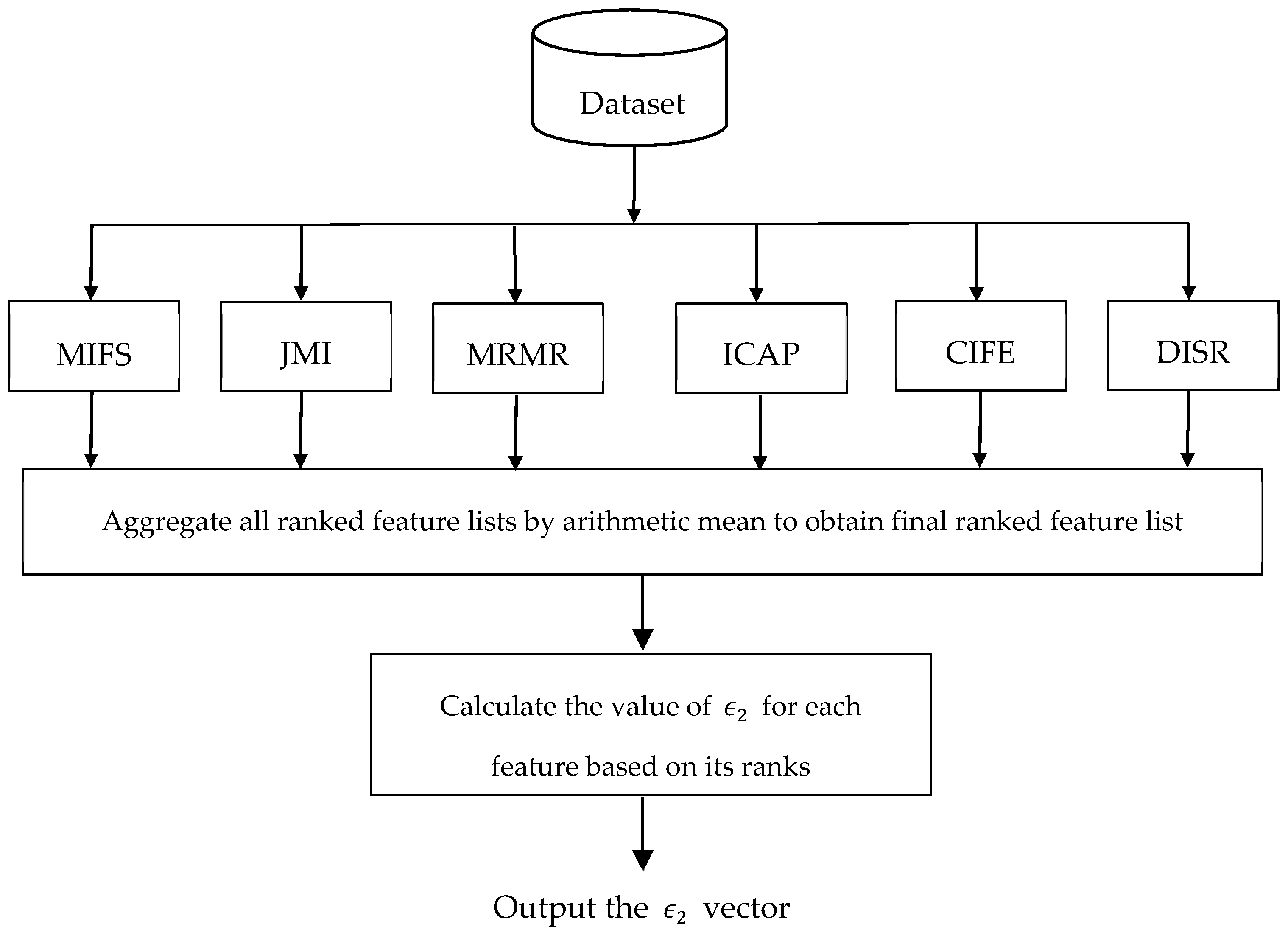
• ${ϵ}_2$ is a vector which their values are used to bias the swarm toward a special part of the search space. If the value of ${ϵ}_2^d$ be near to 0.5, then the chance of choosing the dth feature are equal to the chance of not being selected. In multi-objective feature subset selection, we tend to select fewer features. This means that we tend to generate a particle on that part of the search space in which there exist fewer features. In the other words, we prefer new solutions containing a large number of 0s instead of 1s. In this case, we can set the value of ${ϵ}_2^d$ in the interval [0, 0.5). Note that this simple rule helps the algorithm to find a small number of features which minimize the classification error. To calculate the value of ${ϵ}_2^d$, we recommend using the rank of the dth feature obtained by an ensemble of different filter methods, as discussed in Section 3.4.

3.4. Ensemble of Filter-Based Rankers to Set the Value of ${ϵ}_2$

So far many filter-based rankers have been proposed for feature subset selection. The previous research results confirmed that each filter-based ranker is suitable only for a subset of datasets. In the other words, a filter-based ranker may excellently rank the features of a specific dataset while performing poorly in another dataset. Therefore, choosing the best filter-based ranker for a certain dataset may be difficult due to insufficient knowledge about the dataset and stochastic nature of the data collection process. In the case that we want to use only one filter-based ranker for feature subset selection, it is required to perform the numerous trial-and-error runs to choose a suitable filter algorithm. This approach clearly suffers from high resource consumption, because feature subset selection is a computationally-expensive problem. Motivated by these observations, we propose an ensemble of filter-based rankers which aims to combine the outputs of several filter algorithms in order to reduce the variability of the ranked features and generate a more robust filter algorithm. It is noteworthy that the output of the proposed ensemble method is used as the knowledge about feature importance to intelligently adjust the value of the ${ϵ}_2$ vector.

Figure 1 illustrates the flowchart of calculating the value of the ${ϵ}_2$ vector for features of the dataset. As can be seen in this figure, some ranking lists are generated using different filter-based algorithms for feature ranking, and then these different ranking lists are integrated using the arithmetic mean, where the final score of feature d is calculated by the mean of the ranking scores of this feature in each ranking list. In this paper, we use six filter-based algorithms for feature ranking, including Mutual Information Feature Selection (MIFS) [37], Joint Mutual Information (JMI) [38], Max-Relevance Min-Redundancy (MRMR) [39], Interaction Capping (ICAP) [40], Conditional Infomax Feature Extraction (CIFE) [41], and Double Input Symmetrical Relevance (DISR) [42]. To calculate the value of ${ϵ}_2$ vector, we normalize the final feature ranking vector obtained between 0.01 and 0.1 using the min-max normalization method [6].

3.5. Particle Evaluation

Each meta-heuristic must use a fitness (or cost) evaluation function which associates with each solution of the search space a numeric value that describes its quality. An effective fitness (cost) evaluation function must yield better evaluations to solutions that are closer to the optimal solution than those that are farther away.

Fortunately, the definition of cost evaluation function for wrapper feature subset selection algorithms is straightforward. To evaluate the cost of the feature subset selection and avoid the over-fitting, we use the average error rates of n-fold cross-validation (with n = 10) on training data. In this case, we use the k-nearest neighbors (k-NN) classifier [43] with k = 5 as learning algorithm for wrapper. The k-NN is a type of instance-based machine learning algorithm where its input is the k training instances in the feature space and its output is a class label. In k-NN, an instance is labeled by the majority class of its k nearest neighbors.

3.6. Particle Replacement

In particle replacement step, the generated particle ${\overrightarrow{X}}_{new}\left(t\right)$ is compared with the randomly-selected particle ${\overrightarrow{X}}_r\left(t\right)$. The particle ${\overrightarrow{X}}_{new}\left(t\right)$ is replaced with ${\overrightarrow{X}}_r\left(t\right)$, if its quality is better than it.

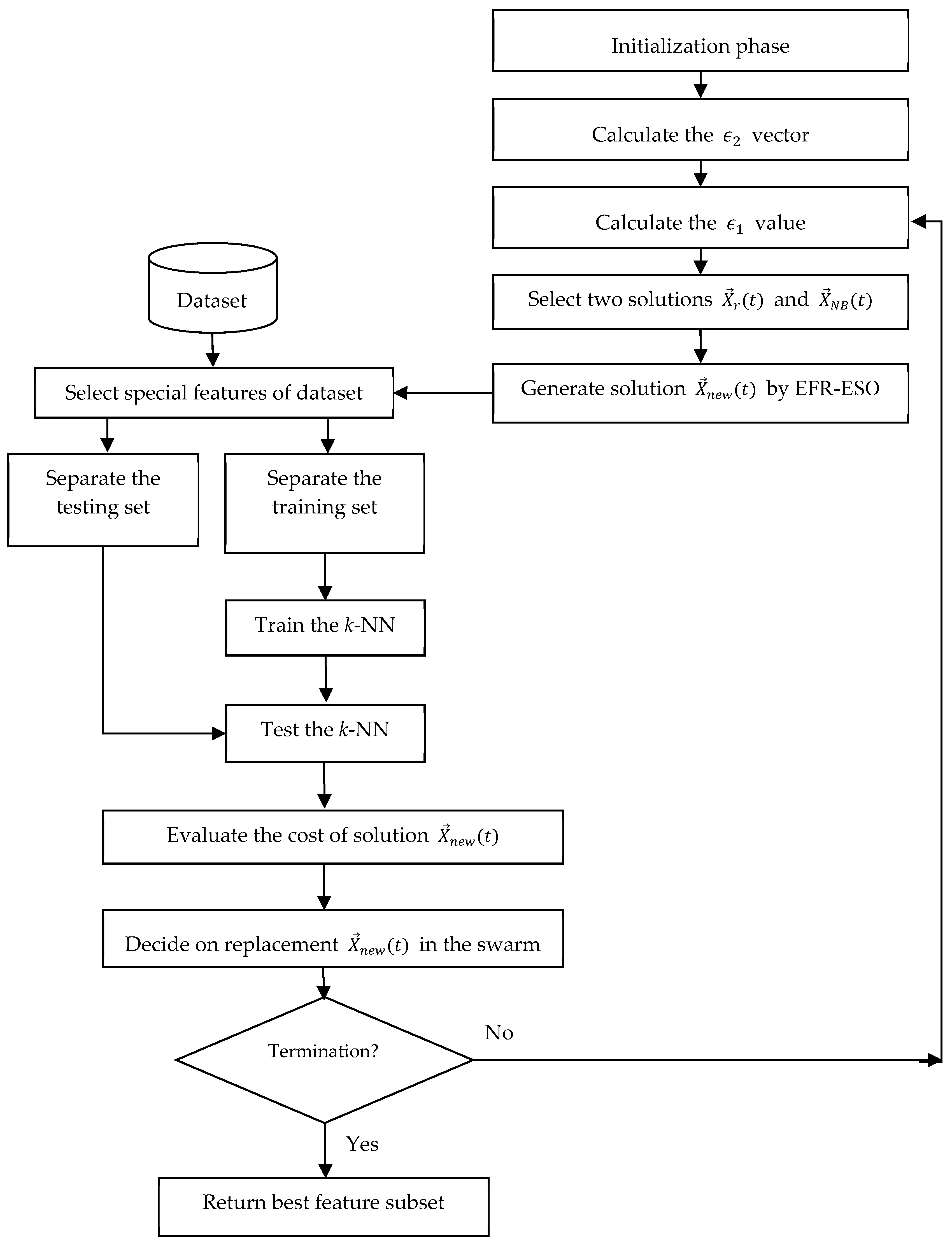
3.7. Algorithmic Details and Flowchart

Algorithm 3 shows the detailed algorithmic steps of proposed EFR-ESO algorithm, and Figure 2 illustrates its system architecture.

Algorithm 3: Outline of EFR-ESO for minimization.

Initialize ${ϵ}_1$(0), N, and stopping criterion; t = 0;   For i = 1 to N Do   Randomly generate the initial solution ${\overrightarrow{X}}_i\left(t\right)$; End for   // feature probabilities calculation: Calculate the rank of each feature by ensemble of filter rankers; Calculate the feature probabilities, i.e., ${ϵ}_2$ vector;   While stopping criterion is not satisfied Do   Update the value of ${ϵ}_1$;     // Particle selection:   Randomly select a particle in the swarm, named ${\overrightarrow{X}}_r\left(t\right)$.   Find the nearest-better neighbor of ${\overrightarrow{X}}_r\left(t\right)$, named ${\overrightarrow{X}}_{NB}\left(t\right)$.   // Particle generation:   For d = 1 to n Do     Generate a random number rand in interval [0, 1];     Update the value of ${ϵ}_2$ by mutual information obtained by filter method;     $x_{new}^d(t)=\{\begin{array}{llll} x_r^d(t),& if\hspace{0.17em}{x}_r^d(t)==x_{NB}^d(t)\hspace{1em}& and& \hspace{1em}rand>{ϵ}_1\\ ~x_r^d(t),& if\hspace{0.17em}{x}_r^d(t)==x_{NB}^d(t)\hspace{1em}& and& \hspace{1em}rand\le {ϵ}_1\\ 0,& if x_r^d(t)\hspace{0.17em}\hspace{0.17em}\ne \hspace{0.17em}\hspace{0.17em}{x}_{NB}^d(t)\hspace{1em}& and& \hspace{1em}rand>{ϵ}_2^d\\ 1,& if x_r^d(t)\hspace{0.17em}\hspace{0.17em}\ne \hspace{0.17em}\hspace{0.17em}{x}_{NB}^d(t)\hspace{1em}& and& \hspace{1em}rand\le {ϵ}_2^d\end{array};$   End for     // Particle replacement:   If $n-fold-cost\left({\overrightarrow{X}}_{new}\left(t\right)\right)<n-fold-cost\left({\overrightarrow{X}}_r\left(t\right)\right)$     ${\overrightarrow{X}}_r\left(t+1\right)={\overrightarrow{X}}_{new}\left(t\right)$;   Else     ${\overrightarrow{X}}_r\left(t+1\right)={\overrightarrow{X}}_r\left(t\right)$;   End if     t = t + 1; End while   Output: The best solution found.

4. Theoretical Convergence Analysis of EFR-ESO Algorithm

In this section, we present the theoretical convergence analysis of the EFR-ESO algorithm based on probability theory. Therefore, we first present the definition of convergence to a global optimum solution, then demonstrate that any feasible solution in the search space can be generated by the EFR-ESO algorithm with a positive probability, and finally prove the global convergence of EFR-ESO algorithm. Denote $x^{*}$ to be a global optimum solution of problem, the global convergence of EFR-ESO algorithm can be defined as follows:

Definition 1.

Let $\{\overrightarrow{X}\left(t\right), t=1,2,\dots \}$ be the sequence of populations in EFR-ESO in each iteration, where $\overrightarrow{X}\left(t\right)=\{{\overrightarrow{X}}_1\left(t\right),\dots ,{\overrightarrow{X}}_N\left(t\right)\}$ is the population in iteration t. It is said that the EFR-ESO algorithm converges to the global optimum solution $x^{*}$, if and only if [44]:

$$\underset{t\to \infty }{\lim }\mathrm{Pr}\{x^{*}\in \overrightarrow{X}\left(t\right)\}=1.$$

(5)

Lemma 1.

For $0<{ϵ}_1<1$ and $0<{ϵ}_2<1$, the EFR-ESO algorithm can generate any feasible solution in each iteration with a probability greater than zero.

Proof. 

Without loss of generality, we consider the process of generation $x_{new}^d\left(t\right)$, which is the dth bit of offspring solution generated at the iteration t + 1. It is shown that for $0<{ϵ}_1<1$ and $0<{ϵ}_2^d<1$, $\mathrm{Pr}\{x_{new}^d\left(t\right)=0\}$ and $\mathrm{Pr}\{x_{new}^d\left(t\right)=1\}$ are greater than zero. Denote $x_r^d\left(t\right)$ to be the dth bit found by the randomly-selected particle at iteration t and $x_{NB}^d\left(t\right)$ to be the dth bit found by the nearest-better particle in the swarm at iteration t. Based on Equation (3), there are three different cases to be investigated:

• If $x_r^d\left(t\right)\ne x_{NB}^d\left(t\right)$, then $\mathrm{Pr}\{x_{new}^d\left(t\right)=0\}=1-{ϵ}_2^d>0$ and $\mathrm{Pr}\{x_{new}^d\left(t\right)=1\}={ϵ}_2^d>0$.
• If $x_r^d\left(t\right)=x_{NB}^d\left(t\right)=1$, then $\mathrm{Pr}\{x_{new}^d\left(t\right)=1\}={ϵ}_1>0$ and $\mathrm{Pr}\{x_{new}^d\left(t\right)=0\}=1-{ϵ}_1>0$.
• If $x_r^d\left(t\right)=x_{NB}^d\left(t\right)=0$, then $\mathrm{Pr}\{x_{new}^d\left(t\right)=0\}={ϵ}_1>0$ and $\mathrm{Pr}\{x_{new}^d\left(t\right)=1\}=1-{ϵ}_1>0$.

Note that because the bit $x_{new}^d\left(t\right)$ is independently generated in the EFR-ESO algorithm, the above cases are satisfied for each solution and each dimension. In conclusion, in each iteration EFR-ESO algorithm can generate any feasible solution of search space $S={\left\{0,1\right\}}^n$ with a probability greater than zero. ☐

Theorem 1.

For $0<{ϵ}_1<1$ and $0<{ϵ}_2^d<1$ the EFR-ESO algorithm converges in probability to the global optimum solution $x^{*}$.

Proof. 

Lemma 1 shows that there exists a probability $p>0$ for generating any feasible solution of search space $S={\left\{0,1\right\}}^n$ in each iteration. Since the global optimum solution $x^{*}$ itself is a feasible solution in $S={\left\{0,1\right\}}^n$, we know that there exists a probability $p>0$ for generating it. Thus, there exists a probability $q=1-p<1$ for not generating $x^{*}$ in each iteration, so:

$$\underset{t\to \infty }{\lim }\mathrm{Pr}\{x^{*}\in \overrightarrow{X}\left(t\right)\}=1-\underset{t\to \infty }{\lim }\mathrm{Pr}\{x^{*}\notin \overrightarrow{X}\left(t\right)\}=1-\underset{t\to \infty }{\lim }{q}^t=1.$$

(6)

☐

5. Experimental Study

In this section, we evaluate the effectiveness of the proposed EFR-ESO algorithm on the high-dimensional feature subset selection problem in terms of both the error rate of the classification and minimizing the number of features. In the following, we first describe the properties of the selected standard benchmarks with and experimental settings. Then, the experimental results of the EFR-ESO algorithm and other several feature subset selection algorithms are described and compared.

5.1. Dataset Properties and Experimental Settings

To evaluate the numerical performance of proposed EFR-ESO algorithm, we performed some experiments on 14 standard high-dimensional datasets, namely, Movement, Musk, Arrhythmia, Madelon, Isolet5, InterAd, Acq, Earn, Melanoma, Lung, Alt, Function, Subcell, and Crohen. The first eight datasets were obtained from UCI repository of Machine Learning databases [45], the next two datasets were obtained from the gene expression omnibus (GEO) [46]. Alt, Function, and Subcell datasets were obtained from [47], and the Crohen dataset was obtained from [48]. The properties of these datasets are listed in

Table 1. Dataset properties.

Dataset	No. of Features	No. of Instances	No. of Calsses
Movement	90	360	15
Musk	167	6598	2
Arrhythmia	279	452	16
Madelon	500	2600	2
Isolet5	617	1559	26
Melanoma	864	57	2
Lung	866	36	2
InterAd	1588	3279	2
Alt	2112	4157	2
Function	2708	3907	2
Subcell	4031	7977	2
Acq	7495	12,897	2
Earn	9499	12,897	2
Crohen	22,283	127	3

. For each dataset, we use 70% samples in the dataset as training data, and the rest for testing. The selection of training and test sets is randomized, while the original ratio of the class distribution is preserved in both sets.

In the comparison, nine algorithms are implemented and tested on MATLAB 2015b (Natick, MA, USA), all based on the well-known k-NN classifier with k = 5. In all comparisons, the standard GA, the Competitive Swarm Optimization (CSO) algorithm [18], the standard PSO, four variants of PSO proposed by Xue’s for bi-objective feature subset selection [23] (Xue1-PSO, Xue2-PSO, Xue3-PSO, and Xue4-PSO), and the Principal Component Analysis (PCA) [6] are compared with the proposed algorithm (EFR-ESO). Based on Xue et al., the major difference between Xue’s algorithms is the number of features selected in the initial swarm, while Xue1-PSO uses the normal initialization method where approximately half of the features are chosen in each particle; Xue2-PSO applies a small initialization method in which only about 10% of the features are chosen in each particle; Xue3-PSO applies a heavy initialization method in which more than half (about 2/3) of the features are chosen in each particle; and Xue4-PSO applies a combined initialization in which a majority (about 2/3) of the particles are initialized with the small initialization method, while the remaining particles of swarm are initialized with the heavy initialization method. Another important difference between Xue’s algorithms and canonical PSO-based algorithms is that, in Xue’s algorithm, the threshold parameter λ is set to 0.6, while this parameter is set to 0.5 as the threshold parameter in canonical PSO.

The population or swarm size is set to 100 for all meta-heuristic algorithms, and the maximal number of fitness evaluation is set to 20,000. Other parameters of the feature subset selection algorithms are: w in the PSO is set to 0.7298, both c1 and c2 in the PSO are set to 1.49618, ϕ in the CSO is set to 0.1, and ${ϵ}_1\left(0\right)$ in the proposed algorithm is set to 0.1. The particles in all algorithms are randomly initialized and the threshold parameter λ = 0.5 is used for both CSO and PSO, while λ = 0.6 is used for Xue’s algorithms. The variance covered in PCA-based feature subset selection is set to 0.95. To obtain statistical results, each algorithm is run 100 times independently.

5.2. Results and Comparisons

Although there are several criteria for assessing the quality of a classifier, the main goal of a classifier is to improve the generalization capability, which means a high accuracy or low misclassification rate on unseen data. Therefore, here we are going to obtain the average error rate or misclassification rate of all the compared feature subset selection algorithms. The generated results by all feature subset selection algorithms are presented in

Table 2. Average error rate.

Dataset	EFR-ESO	GA	CSO	PSO	Xue1-PSO	Xue2-PSO	Xue3-PSO	Xue4-PSO	PCA
Movement	0.1918	0.2861 +	0.2345 +	0.2798 +	0.2846 +	0.2897 +	0.2827 +	0.2853 +	0.2556 +
	(0.0267)	(0.0399)	(0.0398)	(0.0401)	(0.0387)	(0.0436)	(0.0395)	(0.0301)
Musk	0.0012	0.0039 +	0.0010 ≈	0.0038 +	0.0031 +	0.0017 ≈	0.0034 +	0.0014 ≈	0.0028 +
	(0.0010)	(0.0018)	(0.0008)	(0.0021)	(0.0017)	(0.0016)	(0.0015)	(0.0012)
Arrhythmia	0.2991	0.4466 +	0.3222 +	0.4051 +	0.4071 +	0.3484 +	0.4095 +	0.3483 +	0.4491 +
	(0.0203)	(0.0071)	(0.0203)	(0.0217)	(0.0223)	(0.0312)	(0.0238)	(0.0254)
Madelon	0.1253	0.4244 +	0.1545 +	0.4105 +	0.4062 +	0.2712 +	0.4087 +	0.3673 +	0.4812 +
	(0.0203)	(0.0246)	(0.0343)	(0.0177)	(0.0207)	(0.1043)	(0.0214)	(0.0942)
Isolet5	0.1386	0.1866 +	0.1401≈	0.1872 +	0.1853 +	0.1910 +	0.1901 +	0.1803 +	0.4359 +
	(0.0113)	(0.0110)	(0.0105)	(0.0115)	(0.0136)	(0.0142)	(0.0178)	(0.0162)
Melanoma	0.1948	0.2981 +	0.2350 +	0.3173 +	0.3154 +	0.2920 +	0.3064 +	0.2796 +	0.3721 +
	(0.0192)	(0.0296)	(0.0284)	(0.0342)	(0.0491)	(0.0301)	(0.0429)	(0.0307)
Lung	0.2139	0.3312 +	0.2607 +	0.3515 +	0.3603 +	0.3249 +	0.3618 +	0.3242 +	0.3965 +
	(0.0207)	(0.0393)	(0.0236)	(0.0442)	(0.0490)	(0.0405)	(0.0506)	(0.0345)
InterAd	0.0251	0.0405 +	0.0291 +	0.0408 +	0.0397 +	0.0395 +	0.0426 +	0.0483 +	0.0685 +
	(0.0035)	(0.0069)	(0.0052)	(0.0074)	(0.0053)	(0.0048)	(0.0073)	(0.0074)
Alt	0.1224	0.4018 +	0.1647 +	0.4239 +	0.3904 +	0.3727 +	0.4183 +	0.3572 +	0.4215 +
	(0.0135)	(0.0461)	(0.0206)	(0.0490)	(0.0474)	(0.0422)	(0.0445)	(0.0403)
Function	0.2248	0.4259 +	0.2303 ≈	0.4379 +	0.4063 +	0.4403 +	0.4262 +	0.3712 +	0.4539 +
	(0.0196)	(0.0492)	(0.0216)	(0.0504)	(0.0471)	(0.0513)	(0.0473)	(0.0395)
Subcell	0.1650	0.2943 +	0.2071 +	0.2516 +	0.2628 +	0.2816 +	0.2970 +	0.2731 +	0.3604 +
	(0.0179)	(0.0408)	(0.0249)	(0.0325)	(0.0385)	(0.0401)	(0.0468)	(0.0374)
Acq	0.1025	0.2743 +	0.1626 +	0.2708 +	0.2519 +	0.2873 +	0.2917 +	0.2495 +	0.3572 +
	(0.0137)	(0.0399)	(0.0203)	(0.0352)	(0.0371)	(0.0408)	(0.0439)	(0.0375)
Earn	0.0742	0.2902 +	0.1164 +	0.2663 +	0.2836 +	0.2647 +	0.3082 +	0.3125 +	0.3928 +
	(0.0127)	(0.0375)	(0.0195)	(0.0347)	(0.0358)	(0.0317)	(0.0429)	(0.0491)
Crohen	0.1329	0.3265 +	0.1951 +	0.3329 +	0.3014 +	0.3417 +	0.2943 +	0.2758 +	0.4175 +
	(0.0179)	(0.0360)	(0.0268)	(0.0407)	(0.0342)	(0.0381)	(0.0325)	(0.0351)
Better	-	14	11	14	14	13	14	13	14
Worse	-	0	0	0	0	0	0	0	0
Similar	-	0	3	0	0	1	0	1	0

The symbols “⁺”, “^≈”, and “⁻” represent that other methods are statistically inferior to, equal to, or superior to the EFR-ESO algorithm, respectively.

. We also apply the statistical Wilcoxon rank sum test [49] to compare the results of EFR-ESO algorithm and other compared algorithms for feature subset selection. The result is also listed in Table 2, where the symbols “+”, “≈”, and “−” represent that other methods are statistically inferior to, equal to, or superior to the EFR-ESO algorithm, respectively.

The experimental results show that the proposed EFR-ESO has a lower or equal statistical misclassification rate than other compared feature subset selection algorithms on all 14 benchmark datasets. As seen in Table 2, EFR-ESO statistically overcomes the GA, PSO, Xue1-PSO, Xue3-PSO, and PCA on all datasets. Additionally, the proposed algorithm, in most cases, statistically generates better results when compared with other algorithms. Two main reasons for the superiority of the proposed algorithm can be summarized as follows: First, the EFR-ESO is a binary optimization algorithm that is very consistent with the feature subset selection problem. Second, the EFR-ESO does not remove lowly-ranked features from the search process. Therefore, those lowly-ranked features which could increase the accuracy of learning algorithm have a chance to be selected. Based on the generated results, PCA is the least effective algorithm. This could be attributed to the fact that the PCA is sensitive to outliers and noises. In other words, PCA works less efficiently in reducing the accuracy degradation of class-irrelevant attributes.

The removing of all irrelevant and redundant features to improve the classifier is the second goal of the feature subset selection problem. Therefore, we also look at the statistical number of chosen features generated by the compared feature subset selection algorithms. The obtained results are listed in

Table 3. Average number of selected features.

Dataset	EFR-ESO	GA	CSO	PSO	Xue1-PSO	Xue2-PSO	Xue3-PSO	Xue4-PSO	PCA
Movement	21.13	43.12 +	48.21 +	41.25 +	43.04 +	23.04 ≈	51.12 +	40.71 +	10 –
	(4.61)	(5.20)	(6.13)	(5.61)	(6.14)	(6.94)	(7.73)	(13.94)
Musk	8.66	77.41 +	12.27 +	68.79 +	70.37 +	15.45 +	72.47 +	15.72 +	118 +
	(3.92)	(6.94)	(4.62)	(6.54)	(6.94)	(7.24)	(10.37)	(5.59)
Arrhythmia	12.45	150.03 +	15.84 +	130.11 +	131.14 +	21.05 +	150.14 +	26.63 +	106 +
	(7.12)	(12.41)	(6.95)	(9.37)	(12.02)	(11.82)	(13.73)	(26.71)
Madelon	7.19	277.07 +	6.94 ≈	242.52 +	250.94 +	33.02 +	318.63 +	259.16 +	417 +
	(2.03)	(16.83)	(1.93)	(11.70)	(14.91)	(53.12)	(35.72)	(110.61)
Isolet5	97.72	281.22 +	135.15 +	301.12 +	309.52 +	191.38 +	361.93 +	365.47 +	175 +
	(19.07)	(10.05)	(31.07)	(14.72)	(16.07)	(40.72)	(38.17)	(55.13)
Melanoma	15.47	41.65 +	20.52 +	37.93 +	36.13 +	23.18 +	34.92 +	30.44 +	49 +
	(8.93)	(19.23)	(10.29)	(21.16)	(18.65)	(15.75)	(16.35)	(17.32)
Lung	10.25	35.62 +	14.27 +	30.44 +	29.37 +	17.64 +	28.14 +	24.02 +	35 +
	(6.17)	(18.52)	(13.43)	(19.17)	(17.44)	(21.49)	(19.62)	(16.71)
InterAd	197.49	845.61 +	267.63 +	755.48 +	763.71 +	388.10 +	892.04 +	928.19 +	286 +
	(72.01)	(42.02)	(92.48)	(26.72)	(36.68)	(83.16)	(98.51)	(151.26)
Alt	29.62	986.53 +	40.12 +	948.72 +	990.16 +	338.27 +	957.35 +	913.07 +	1204 +
	(12.43)	(61.49)	(15.89)	(55.04)	(61.82)	(36.70)	(63.93)	(65.19)
Function	32.76	1207.45 +	51.37 +	1049.28 +	1102.70 +	504.56 +	1319.52 +	1174.21 +	1973 +
	(15.85)	(89.26)	(19.42)	(84.50)	(88.46)	(47.91)	(95.02)	(81.49)
Subcell	40.16	1952.37 +	49.37 +	1775.91 +	2004.94 +	916.68 +	1873.64 +	1804.26 +	2735 +
	(15.93)	(112.04)	(16.30)	(109.78)	(119.73)	(79.83)	(118.33)	(129.37)
Acq	51.49	3093.46 +	63.92 +	2714.05 +	2993.18 +	1329.41 +	2813.20 +	2951.40 +	4512 +
	(21.70)	(162.14)	(28.03)	(150.11)	(175.72)	(95.37)	(152.74)	(146.38)
Earn	75.42	4617.25 +	102.17 +	4056.44 +	4713.56 +	2021.52 +	4396.61 +	4301.07 +	6132 +
	(23.59)	(207.11)	(31.54)	(195.71)	(219.50)	(124.13)	(197.24)	(219.14)
Crohen	118.61	8752.73 +	144.07 +	8126.83 +	7815.91 +	3406.15 +	7916.75 +	8001.25 +	12,740 +
	(38.72)	(469.52)	(45.41)	(443.25)	(401.49)	(194.60)	(420.93)	(412.48)
Better	-	14	13	14	14	13	14	14	13
Worse	-	0	0	0	0	0	0	0	1
Similar	-	0	1	0	0	1	0	0	0

The symbols “⁺”, “^≈”, and “^–” represent that other methods are statistically inferior to, equal to, or superior to the EFR-ESO algorithm, respectively.

. In this comparison, it is visible that the proposed EFR-ESO chooses fewer average features than most compared algorithms for feature subset selection. The main reason for this superiority is that the irrelevant features have little chance of being selected, and many of them are not selected during the search due to their inefficiencies in classification. From Table 3, it is visible that the number of features chosen by the PSO-based algorithms are proportional to the number of features initialized in the first generation. In other words, if we initialize the particles of swarm with a small number of features, the number of features chosen in the final swarm will be smaller, and vice versa. By contrast, EFR-ESO is not sensitive to the number of features initialized in the first iteration, which can always find the near-optimal feature subset regardless the number of features chosen during the particle initialization phase.

6. Conclusions and Future Work

In this paper, we propose a novel hybrid filter-wrapper algorithm, called Ensemble of Filter-based Rankers to guide an Epsilon-greedy Swarm Optimizer (EFR-ESO), for solving high-dimensional feature subset selection. The Epsilon-greedy Swarm Optimizer (ESO) is a novel binary swarm intelligence algorithm introduced in this paper as a novel wrapper. In each iteration of the ESO, a particle is randomly selected, then the nearest-better neighbor of this particle in the swarm is found and, finally, a new particle is created based on these particles using a new epsilon-greedy method. If the quality of new particle is better than the randomly-selected particle, new particle is replaced in the swarm, otherwise the new particle is discarded. In the proposed EFR-ESO, we extract the knowledge about the feature importance by the ensemble of filter-based rankers and then use this knowledge to weight the feature probabilities in the ESO. Experiments on 14 datasets indicate that the proposed algorithm has a great performance on high-dimensional feature subset selection in terms of both the error rate of the classification and minimizing the number of features.

For future research, the proposed algorithm can be studied on other real-world binary optimization problems, such as the 0/1 knapsack problem, Winner Determination Problem (WDP) in multi-agent systems, and so on. Additionally, the effectiveness of the proposed algorithm for solving the multi-objective feature subset selection with the approach of finding the Pareto front can be investigated. Finally, one can research how to build a new solution in the search space, which can have an effective control between diversity and convergence.

References

1. Chandrashekar, G.; Sahin, F. A survey on feature selection methods. Comput. Electr. Eng. 2014, 40, 16–28. [Google Scholar] [CrossRef]
2. Gheyas, I.A.; Smith, L.S. Feature subset selection in large dimensionality domains. Pattern Recognit. 2010, 43, 5–13. [Google Scholar] [CrossRef]
3. Garey, M.R.; Johnson, D.S. A Guide to the Theory of NP-Completeness, 1st ed.; WH Freemann: New York, NY, USA, 1979. [Google Scholar]
4. Xue, B.; Zhang, M.; Browne, W.N.; Yao, X. A survey on evolutionary computation approaches to feature selection. IEEE Ttans. Evolut. Comput. 2016, 20, 606–626. [Google Scholar] [CrossRef]
5. Pudil, P.; Novovičová, J.; Kittler, J. Floating search methods in feature selection. Pattern Recogn Lett. 1994, 15, 1119–1125. [Google Scholar] [CrossRef]
6. Alpaydin, E. Introduction to Machine Learning, 3rd ed.; MIT Press: Cambridge, MA, USA, 2014. [Google Scholar]
7. Talbi, E.G. Meta-Heuristics: From Design to Implementation; John Wiley & Sons: Hoboken, NJ, USA, 2009. [Google Scholar]
8. Han, K.H.; Kim, J.H. Quantum-inspired evolutionary algorithm for a class of combinatorial optimization. IEEE Trans. Evolut. Comput. 2002, 6, 580–593. [Google Scholar] [CrossRef]
9. Banks, A.; Vincent, J.; Anyakoha, C. A review of particle swarm optimization. Part II: Hybridisation, combinatorial, multicriteria and constrained optimization, and indicative applications. Nat. Comput. 2008, 7, 109–124. [Google Scholar] [CrossRef]
10. Cheng, R.; Jin, Y. A competitive swarm optimizer for large scale optimization. IEEE Trans. Cybern. 2015, 45, 191–204. [Google Scholar] [CrossRef] [PubMed]
11. Dowlatshahi, M.B.; Rezaeian, M. Training spiking neurons with gravitational search algorithm for data classification. In Proceedings of the Swarm Intelligence and Evolutionary Computation (CSIEC), Bam, Iran, 9–11 March 2016; pp. 53–58. [Google Scholar]
12. Dowlatshahi, M.B.; Derhami, V. Winner Determination in Combinatorial Auctions using Hybrid Ant Colony Optimization and Multi-Neighborhood Local Search. J. AI Data Min. 2017, 5, 169–181. [Google Scholar]
13. Siedlecki, W.; Sklansky, J. A note on genetic algorithms for large-scale feature selection. Pattern Recognit Lett. 1989, 10, 335–347. [Google Scholar] [CrossRef]
14. Li, Y.; Zhang, S.; Zeng, X. Research of multi-population agent genetic algorithm for feature selection. Expert Syst. Appl. 2009, 36, 11570–11581. [Google Scholar] [CrossRef]
15. Kabir, M.M.; Shahjahan, M.; Murase, K. A new local search based hybrid genetic algorithm for feature selection. Neurocomputing 2011, 74, 2914–2928. [Google Scholar] [CrossRef]
16. Huang, C.L.; Dun, J.F. A distributed PSO–SVM hybrid system with feature selection and parameter optimization. Appl. Soft Comput. 2008, 8, 1381–1391. [Google Scholar] [CrossRef]
17. Chuang, L.Y.; Yang, C.H.; Li, J.C. Chaotic maps based on binary particle swarm optimization for feature selection. Appl. Soft Comput. 2011, 11, 239–248. [Google Scholar] [CrossRef]
18. Zhang, Y.; Wang, S.; Phillips, P.; Ji, G. Binary PSO with mutation operator for feature selection using decision tree applied to spam detection. Knowl.-Based Syst. 2014, 64, 22–31. [Google Scholar] [CrossRef]
19. Gu, S.; Cheng, R.; Jin, Y. Feature selection for high-dimensional classification using a competitive swarm optimizer. Soft Comput. 2016, 1–12. [Google Scholar] [CrossRef]
20. Tanaka, K.; Kurita, T.; Kawabe, T. Selection of import vectors via binary particle swarm optimization and cross-validation for kernel logistic regression. In Proceedings of the International Joint Conference on Networks, Orlando, FL, USA, 12–17 August 2007. [Google Scholar]
21. Wang, X.; Yang, J.; Teng, X.; Xia, W.; Jensen, R. Feature selection based on rough sets and particle swarm optimization. Pattern Recognit. Lett. 2007, 28, 459–471. [Google Scholar] [CrossRef] [Green Version]
22. Sahu, B.; Mishra, D. A novel feature selection algorithm using particle swarm optimization for cancer microarray data. Procedia Eng. 2012, 38, 27–31. [Google Scholar] [CrossRef]
23. Xue, B.; Zhang, M.; Browne, W.N. Particle swarm optimization for feature selection in classification: A multi-objective approach. IEEE Trans. Cybern. 2013, 43, 1656–1671. [Google Scholar] [CrossRef] [PubMed]
24. Zhou, X.X.; Zhang, Y.; Ji, G.; Yang, J.; Dong, Z.; Wang, S.; Phillips, P. Detection of abnormal MR brains based on wavelet entropy and feature selection. IEEJ Trans. Electr. Electron. Eng. 2016, 11, 364–373. [Google Scholar] [CrossRef]
25. Emary, E.; Zawbaa, H.M.; Hassanien, A.E. Binary ant lion approaches for feature selection. Neurocomputing 2016, 213, 54–65. [Google Scholar] [CrossRef]
26. Zawbaa, H.M.; Emary, E.; Grosan, C. Feature selection via chaotic antlion optimization. PLoS ONE 2016, 11, e0150652. [Google Scholar] [CrossRef] [PubMed]
27. Shunmugapriya, P.; Kanmani, S. A hybrid algorithm using ant and bee colony optimization for feature selection and classification (AC-ABC Hybrid). Swarm Evolut. Comput. 2017, 36, 27–36. [Google Scholar] [CrossRef]
28. Bello, R.; Gomez, Y.; Garcia, M.M.; Nowe, A. Two-step particle swarm optimization to solve the feature selection problem. In Proceedings of the 7th International Conference on Intelligent Systems Design and Applications, Rio de Janeiro, Brazil, 22–24 October 2007; pp. 691–696. [Google Scholar]
29. Oreski, S.; Oreski, G. Genetic algorithm-based heuristic for feature selection in credit risk assessment. Expert Syst. Appl. 2014, 41, 2052–2064. [Google Scholar] [CrossRef]
30. Tan, F.; Fu, X.Z.; Zhang, Y.Q.; Bourgeois, A. A genetic algorithm based method for feature subset selection. Soft Comput. 2008, 12, 111–120. [Google Scholar] [CrossRef]
31. Han, J.; Pei, J.; Kamber, M. Data Mining: Concepts and Techniques, 3rd ed.; Elsevier: Waltham, MA, USA, 2011. [Google Scholar]
32. Liu, H.L.; Chen, L.; Deb, K.; Goodman, E.D. Investigating the effect of imbalance between convergence and diversity in evolutionary multi-objective algorithms. IEEE Trans. Evolut. Comput. 2017, 21, 408–425. [Google Scholar] [CrossRef]
33. Dowlatshahi, M.B.; Nezamabadi-Pour, H.; Mashinchi, M. A discrete gravitational search algorithm for solving combinatorial optimization problems. Inf. Sci. 2014, 258, 94–107. [Google Scholar] [CrossRef]
34. Rafsanjani, M.K.; Dowlatshahi, M.B. A Gravitational search algorithm for finding near-optimal base station location in two-tiered WSNs. In Proceedings of the 3rd International Conference on Machine Learning and Computing, Singapore, 26–28 February 2011; pp. 213–216. [Google Scholar]
35. Črepinšek, M.; Liu, S.H.; Mernik, M. Exploration and exploitation in evolutionary algorithms: A survey. ACM Comput. Surv. 2013, 45, 1–35. [Google Scholar] [CrossRef]
36. Mahdavi, S.; Rahnamayan, S.; Deb, K. Opposition based learning: A literature review. Swarm Evolut. Comput. 2017. [Google Scholar] [CrossRef]
37. Battiti, R. Using mutual information for selecting features in supervised neural net learning. IEEE Trans. Neural Netw. 1994, 5, 537–550. [Google Scholar] [CrossRef] [PubMed]
38. Yang, H.; Moody, J. Data visualization and feature selection: New algorithms for non-gaussian data. In Advances in Neural Information Processing Systems; Walker Road: Beaverton, OR, USA, 1999; pp. 687–693. [Google Scholar]
39. Peng, H.; Long, F.; Ding, C. Feature selection based on mutual information: Criteria of max-dependency, max-relevance, and min-redundancy. IEEE Trans. Pattern Anal. Mach. Intell. 2005, 27, 1226–1238. [Google Scholar] [CrossRef] [PubMed]
40. Jakulin, A. Machine Learning Based on Attribute Interactions. Ph.D. Thesis, University of Ljubljana, Ljubljana, Slovenia, 2005. [Google Scholar]
41. Lin, D.; Tang, X. Conditional infomax learning: An integrated framework for feature extraction and fusion. In Proceedings of the 9th European Conference on Computer Vision, Graz, Austria, 7–13 May 2006. [Google Scholar]
42. Meyer, P.; Bontempi, G. On the use of variable complementarity for feature selection in cancer classification. In Evolutionary Computation and Machine Learning in Bioinformatics; Springer: Berlin/Heidelberg, Germany, 2006; pp. 91–102. [Google Scholar]
43. Abbasifard, M.R.; Ghahremani, B.; Naderi, H. A survey on nearest neighbor search methods. Int. J. Comput. Appl. 2014, 95, 39–52. [Google Scholar]
44. Chen, Y.; Xie, W.; Zou, X. A binary differential evolution algorithm learning from explored solutions. Neurocomputing 2015, 149, 1038–1047. [Google Scholar] [CrossRef]
45. UCI Repository of Machine Learning Databases. Available online: http://www.ics.uci.edu/mlearn/MLRepository.html (accessed on 22 September 2017).
46. Gene Expression Omnibus (GEO). Available online: https://www.ncbi.nlm.nih.gov/geo/ (accessed on 19 October 2017).
47. Mitchell, A.L.; Divoli, A.; Kim, J.H.; Hilario, M.; Selimas, I.; Attwood, T.K. METIS: Multiple extraction techniques for informative sentences. Bioinformatics 2005, 21, 4196–4197. [Google Scholar] [CrossRef] [PubMed]
48. Burczynski, M.E.; Peterson, R.L.; Twine, N.C.; Zuberek, K.A.; Brodeur, B.J.; Casciotti, L.; Maganti, V.; Reddy, P.S.; Strahs, A.; Immermann, F.; et al. Molecular classification of Crohn’s disease and ulcerative colitis patients using transcriptional profiles in peripheral blood mononuclear cells. J. Mol. Diagn. 2006, 8, 51–61. [Google Scholar] [CrossRef] [PubMed]
49. Derrac, J.; García, S.; Molina, D.; Herrera, F. A practical tutorial on the use of nonparametric statistical tests as a methodology for comparing evolutionary and swarm intelligence algorithms. Swarm Evolut. Comput. 2011, 1, 3–18. [Google Scholar] [CrossRef]
Figure 1. Flowchart of the ensemble of feature rankers to calculate the ϵ 2 vector.
Information 08 00152 g001
Figure 2. System architecture of the proposed EFR-ESO algorithm for feature subset selection.
Information 08 00152 g002