
Round Robin Testing: Exploring Experimental Uncertainties through a Multifacility Comparison of a Hinged Raft Wave Energy Converter

 , , , , , ,
  , , , ,
  ,
,  ,
,  and
and
Abstract
:1. Introduction
2. Model and Experimental Design
2.1. Hinged Raft WEC Model Properties
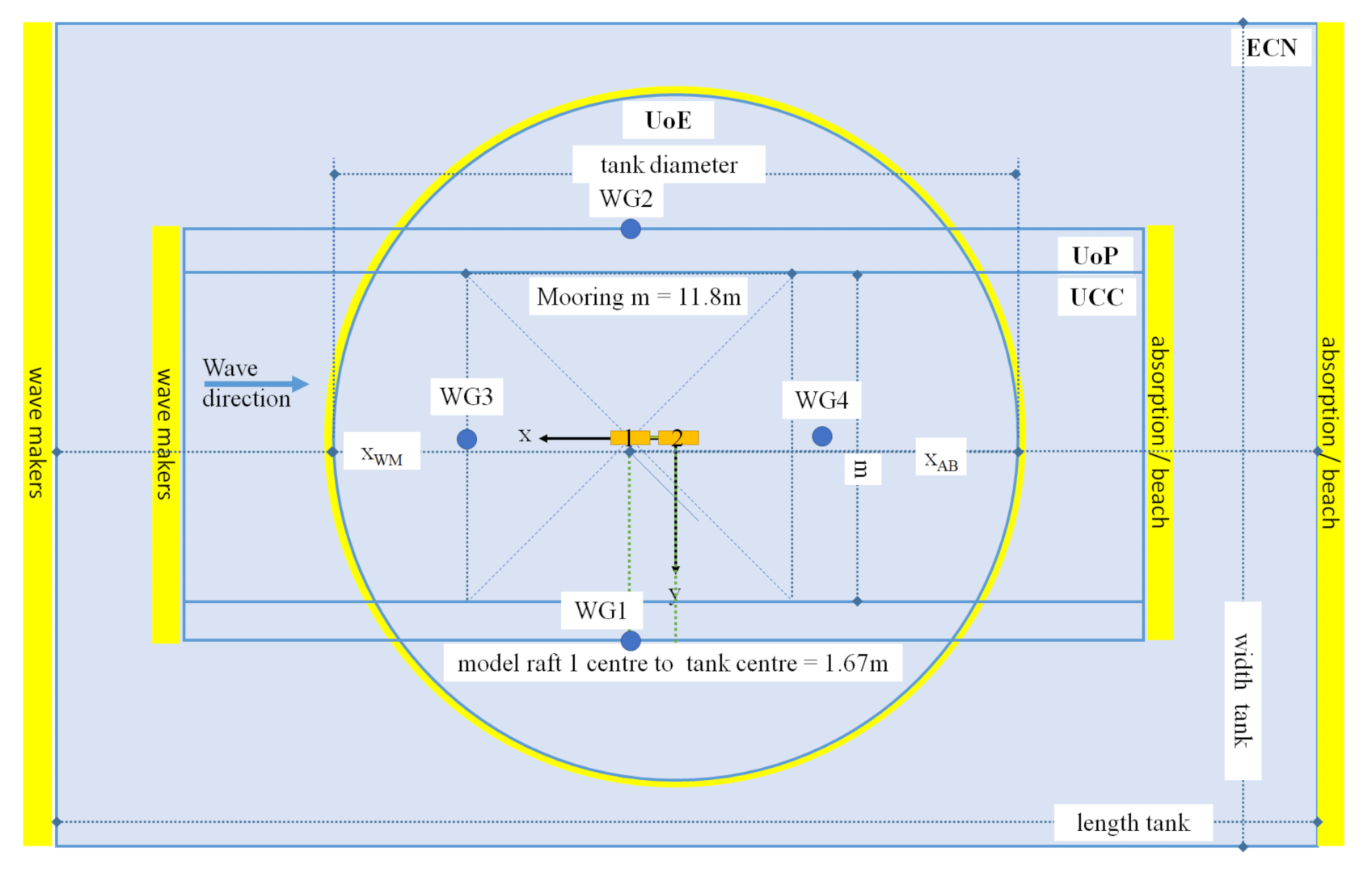
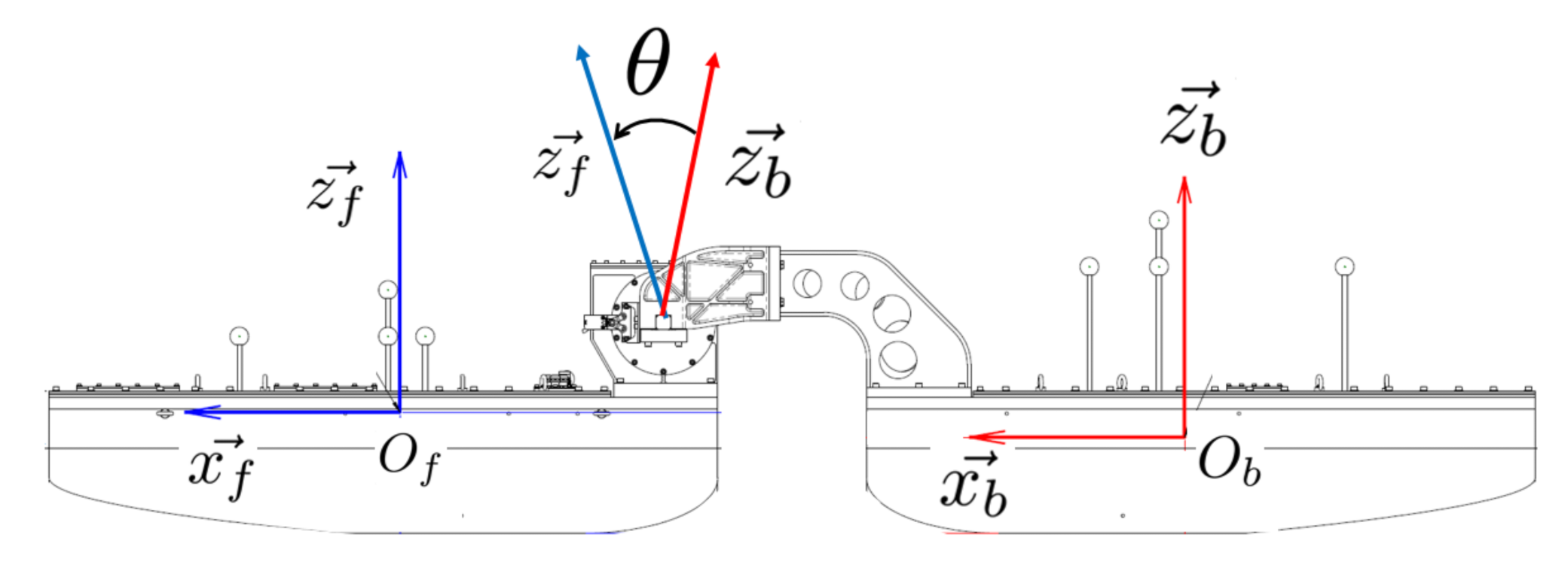
2.2. Model Axes
2.3. Power Takeoff
2.4. Measurement and Instrumentation
2.4.1. Model Instruments and Data Acquisition
2.4.2. Motion Capture
2.4.3. Wave Measurement
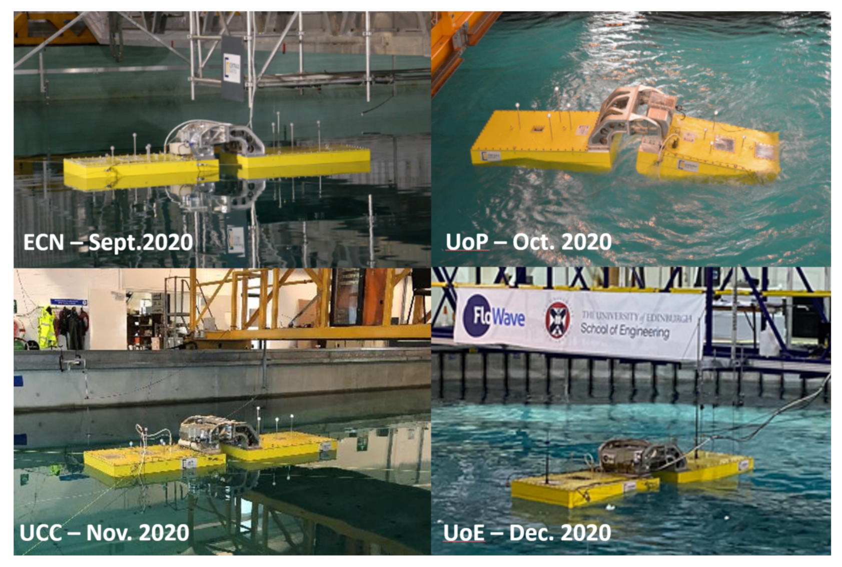
2.5. Facilities
2.5.1. Centrale Nantes
2.5.2. University of Plymouth
2.5.3. University College Cork
2.5.4. University of Edinburgh
2.6. Sea States
3. Analysis and Results
3.1. Key Parameters
- Environmental conditions (i.e., sea state calibration);
- Device motions (of fore/aft rafts and the hinge angle);
- Mooring loads;
- Power output.
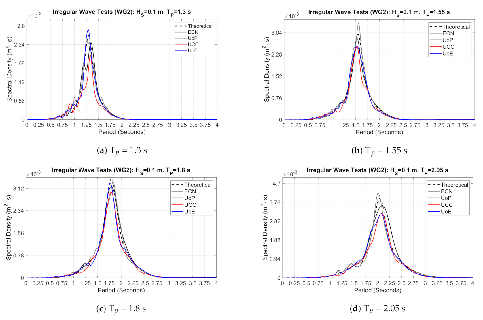
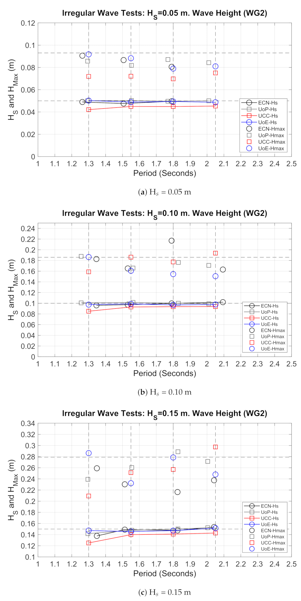
3.2. Sea States
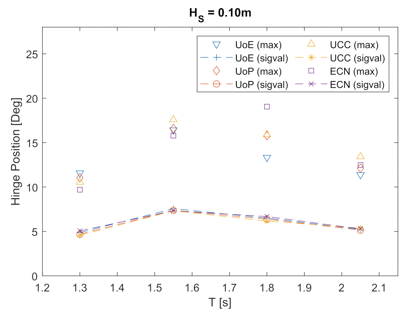
3.3. Hinge Position
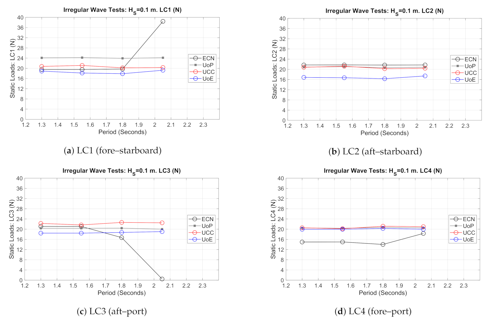
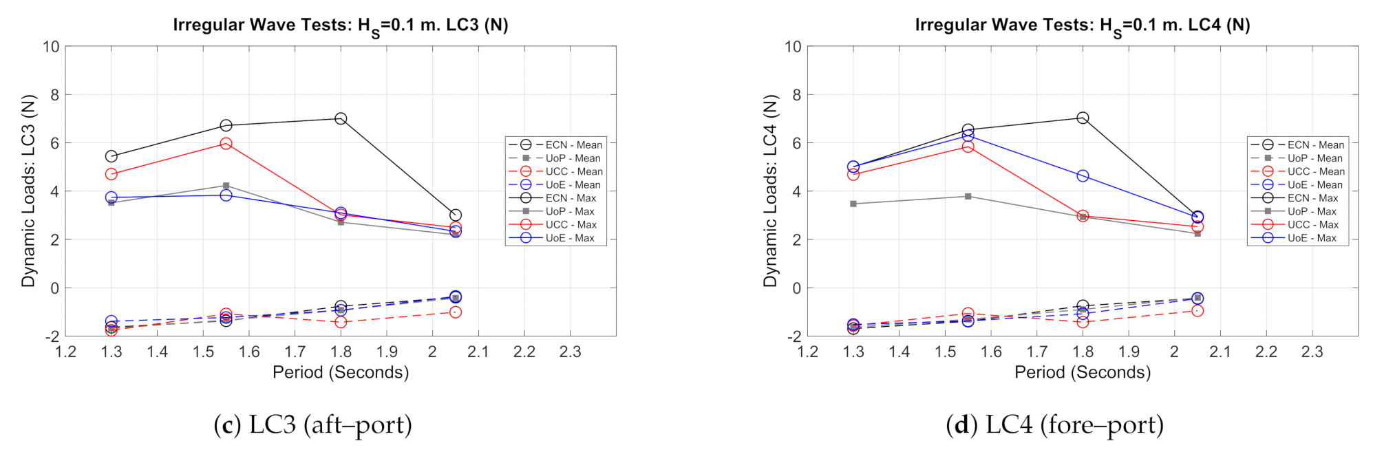
3.4. Mooring Loads
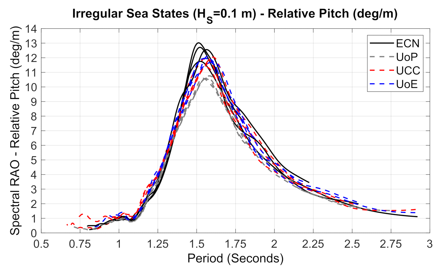
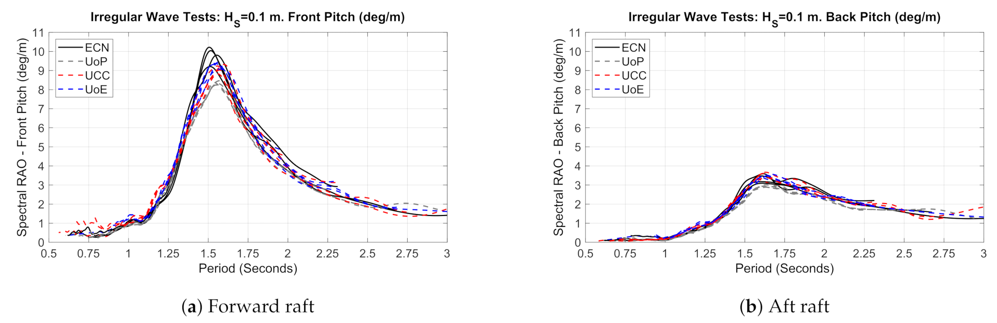
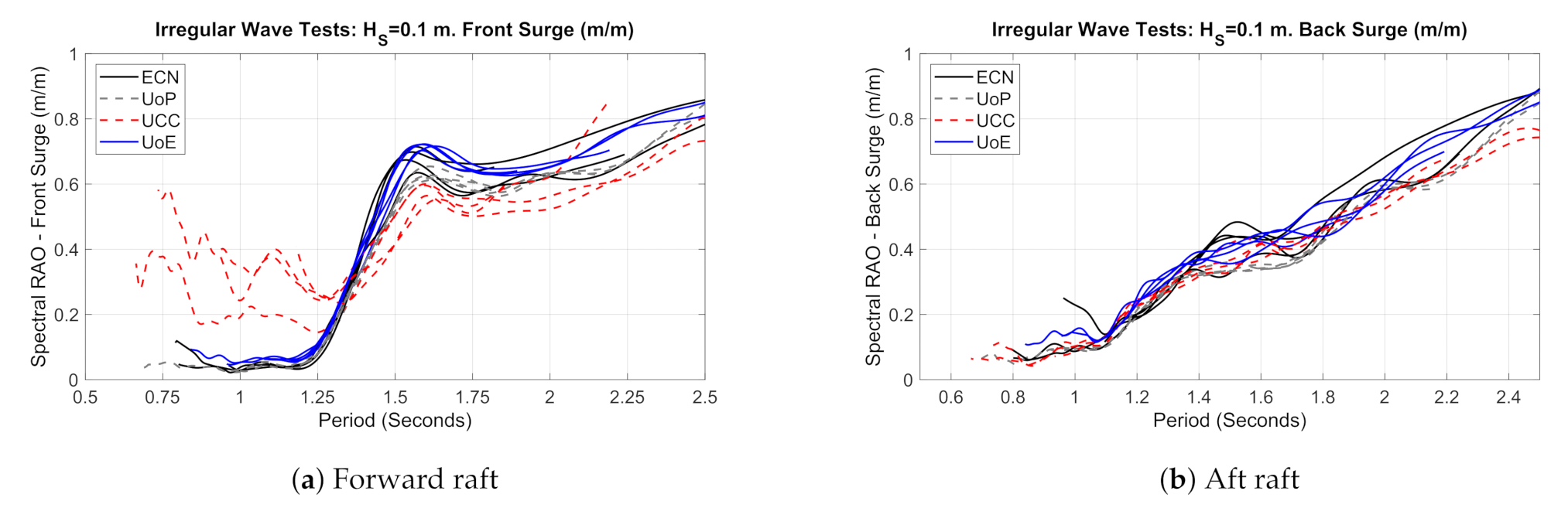
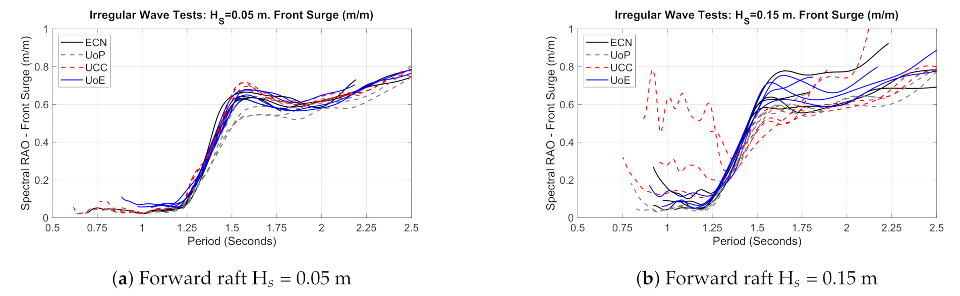
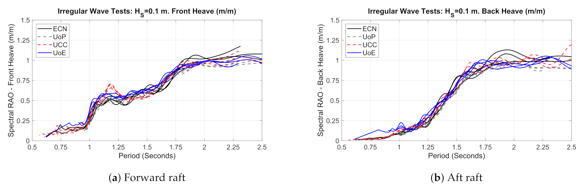
3.5. Motions: Pitch, Heave and Surge
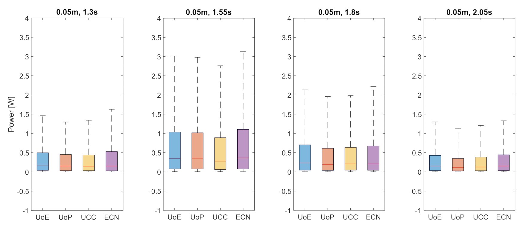
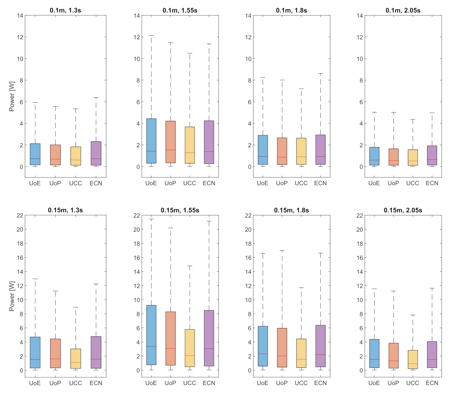
3.6. Power
4. Discussion
4.1. Variability of Motions, Loads and Power
4.2. Influence of Experimental Setup and Calibration
- Operational calibrations conducted using spectra averaged across multiple gauges to minimise the influence of hotspots and reflections;
- Inconsistency in facility procedures between using incident spectra (obtained through multigauge reflection analysis) vs. total spectra;
- Differences in facility procedures in terms of accepted uncertainty.
4.3. Recommendations for WEC Tank Testing Consistency
- Sea state characterisation should be clearly reported along with the facility’s methodology. It must be clear whether the values relate to total or incident spectrum;
- Where possible, the characterisation should be based on an average of 3–5 wave gauges measuring in the absence of the model (“open tank”). These gauges would typically cover the area occupied by the model, suggesting a footprint of 1–2 m. The gauges may be spaced to support reflection analysis, allowing the incident spectrum to be reported;
- As a minimum, the H value from the total spectrum should be reported as averaged across the gauges. It is noted that wave periods in contemporary wave tanks are reproduced very accurately; nevertheless, it may be desirable to report mean periods as a measure of quality assurance. Full reporting requirements were outlined in [10] as recommended by the IEC;
- Where reflection analysis is conducted, the incident parameters may be reported alongside the total spectrum. The reflection analysis methodology should also be referenced.
- Accurate characterisation of the sea state is considered as a prerequisite to any sea state calibration. An established facility with experienced operators is likely to be capable of producing sea states to within 5% of the target values with no (or minimal) iteration. In a time-limited programme, it may therefore be acceptable to run uncalibrated sea states, provided they are characterised as detailed above;
- Where sea state calibration is conducted, the methodology must be reported, in particular the adjustments made to the input spectrum. For example, is the target achieved through the application of a broad gain function, or is a frequency-dependent gain function applied (adjusting each frequency bin individually)? The latter method is recommended where practical. It is suggested that a standardised procedure should be adopted (e.g., by the IEC) for sea state characterisation and calibration given its clear importance for maintaining consistency between laboratories. This influence was even more pronounced on the parallel regular wave tests that accompanied the work reported here;
- The use of a design wave (i.e., recreating a specific time series at the model location) should be considering as a benchmarking tool to aid comparison between test programmes at different facilities. It is also recommended that this approach be considered for any future round robin test programmes;
- Assuming that the model itself maintains consistency between programmes, the key source of variability is the interface with the facility (e.g., the moorings). In addition to ensuring dimensional accuracy, it is suggested that pull tests, to establish the stiffness of the system, be conducted.
4.4. Dataset Availability and Applications
5. Conclusions
Author Contributions
Funding
Data Availability Statement
Acknowledgments
Conflicts of Interest
Abbreviations
| DoF | Degree of freedom |
| IEC | International Electrotechnical Commission |
| IQR | Interquartile range |
| JONSWAP | Joint North Sea Wave Project |
| MoCAP | Motion capture |
| PTO | Power takeoff |
| RAO | Response amplitude operator |
| TRL | Technology readiness level |
| WEC | Wave energy converter |
| WG | Wave gauge |
| WM | Wave maker |
Appendix A. Kruskal–Wallis and Mann–Whitney U Tests: Analysis of Power

| H [m] | T [s] | |||
|---|---|---|---|---|
| 1.3 | 1.55 | 1.8 | 2.05 | |
| 0.05 | 1.18 × | 7.85 × | 2.58 × | 8.43 × |
| 0.1 | 2.87 × | 2.17 × | 5.53 × | 7.02 × |
| 0.15 | 1.96 × | 8.36 × | 2.09 × | 2.33 × |
| H [m] | T = 1.3 s | ||||
|---|---|---|---|---|---|
| UoE | UoP | UCC | ECN | ||
| 0.05 | UoE | 3.11 × | 1.72 × | 5.28 × | |
| UoP | 3.11 × | 4.97 × | 2.41 × | ||
| UCC | 1.72 × | 4.97 × | 5.55 × | ||
| ECN | 5.28 × | 2.41 × | 5.55 × | ||
| 0.1 | UoE | 3.21 × | 2.32 × | 4.61 × | |
| UoP | 3.21 × | 1.92 × | 1.21 × | ||
| UCC | 2.32 × | 1.92 × | 4.58 × | ||
| ECN | 4.61 × | 1.21 × | 4.58 × | ||
| 0.15 | UoE | 1.34 × | 1.06 × | 6.90 × | |
| UoP | 1.34 × | 9.44 × | 9.53 × | ||
| UCC | 1.06 × | 9.44 × | 1.01 × | ||
| ECN | 6.90 × | 9.53 × | 1.01 × | ||
| H [m] | T = 1.55 s | ||||
|---|---|---|---|---|---|
| UoE | UoP | UCC | ECN | ||
| 0.05 | UoE | 7.55 × | 1.87 × | 3.17 × | |
| UoP | 7.55 × | 4.24 × | 3.72 × | ||
| UCC | 1.87 × | 4.24 × | 1.49 × | ||
| ECN | 3.17 × | 3.72 × | 1.49 × | ||
| 0.1 | UoE | 7.16 × | 2.61 × | 1.58 × | |
| UoP | 7.16 × | 2.87 × | 2.68 × | ||
| UCC | 2.61 × | 2.87 × | 2.04 × | ||
| ECN | 1.58 × | 2.68 × | 2.04 × | ||
| 0.15 | UoE | 2.57 × | 9.70 × | 5.49 × | |
| UoP | 2.57 × | 3.13 × | 5.85 × | ||
| UCC | 9.70 × | 3.13 × | 4.94 × | ||
| ECN | 5.49 × | 5.85 × | 4.94 × | ||
| H [m] | T = 1.8 s | ||||
|---|---|---|---|---|---|
| UoE | UoP | UCC | ECN | ||
| 0.05 | UoE | 2.08 × | 2.41 × | 5.06 × | |
| UoP | 2.08 × | 3.63 × | 1.42 × | ||
| UCC | 2.41 × | 3.63 × | 3.85 × | ||
| ECN | 5.06 × | 1.42 × | 3.85 × | ||
| 0.1 | UoE | 3.70 × | 2.78 × | 3.59 × | |
| UoP | 3.70 × | 3.14 × | 1.17 × | ||
| UCC | 2.78 × | 3.14 × | 5.19 × | ||
| ECN | 3.59 × | 1.17 × | 5.19 × | ||
| 0.15 | UoE | 2.48 × | 1.75 × | 7.29 × | |
| UoP | 2.48 × | 7.27 × | 5.67 × | ||
| UCC | 1.75 × | 7.27 × | 2.47 × | ||
| ECN | 7.29 × | 5.67 × | 2.47 × | ||
| H [m] | T = 2.05 s | ||||
|---|---|---|---|---|---|
| UoE | UoP | UCC | ECN | ||
| 0.05 | UoE | 5.73 × | 4.55 × | 1.74× | |
| UoP | 5.73 × | 2.18 × | 5.28 × | ||
| UCC | 4.55 × | 2.18 × | 1.51 × | ||
| ECN | 1.74 × | 5.28 × | 1.51 × | ||
| 0.1 | UoE | 2.15 × | 9.30 × | 1.42 × | |
| UoP | 2.15 × | 1.23 × | 4.45 × | ||
| UCC | 9.30 × | 1.23 × | 2.02 × | ||
| ECN | 1.42 × | 4.45 × | 2.02 × | ||
| 0.15 | UoE | 3.44 × | 4.63 × | 2.66 × | |
| UoP | 3.44 × | 5.87 × | 5.20 × | ||
| UCC | 4.63 × | 5.87 × | 1.81 × | ||
| ECN | 2.66 × | 5.20 × | 1.81 × | ||
References
- Martinez, R.; Gaurier, B.; Ordonez-Sanchez, S.; Facq, J.V.; Germain, G.; Johnstone, C.; Santic, I.; Salvatore, F.; Davey, T.; Old, C.; et al. Tidal Energy Round Robin Tests: A Comparison of Flow Measurements and Turbine Loading. J. Mar. Sci. Eng. 2021, 9, 425. [Google Scholar] [CrossRef]
- Ohana, J.; Gueydon, S.; Judge, F.; Haquin, S.; Weber, M.; Lyden, E.; Thiebaut, F.; O’Shea, M.; Murphy, J.; Davey, T.; et al. Round robin tests on hinged raft wave energy converter. In Proceedings of the EWTEC 2021, Plymouth, UK, 5–9 September 2021. [Google Scholar]
- Qiu, W.; Meng, W.; Peng, H.; Li, J.; Rousset, J.M.; Rodríguez, C.A. Benchmark data and comprehensive uncertainty analysis of two-body interaction model tests in a towing tank. Ocean Eng. 2019, 171, 663–676. [Google Scholar] [CrossRef]
- Robertson, A.N.; Bachynski, E.E.; Gueydon, S.; Wendt, F.; Schünemann, P.; Jonkman, J. Assessment of Experimental Uncertainty for a Floating Wind Semisubmersible Under Hydrodynamic Loading. In Proceedings of the International Conference on Offshore Mechanics and Arctic Engineering, Madrid, Spain, 17–22 June 2018. [Google Scholar] [CrossRef]
- Uncertainty Analysis for a Wave Energy Converter. Procedure 7.5-02-07-03.12. Technical Report. ITCC. 2017. Available online: https://ittc.info/media/2021/75-02-02-02.pdf (accessed on 30 August 2021).
- Payne, G. Guidance for Experimental Tank Testing of Wave Energy Converters; Technical Report, SuperGen Marine; The University of Edinburgh: Edinburgh, UK, 2008; Available online: https://www.supergen-marine.org.uk/sites/supergen-marine.org.uk/files/publications/WEC_tank_testing.pdf (accessed on 30 August 2021).
- Lamont-Kane, P.; Folley, M.; Whittaker, T. Investigating uncertainties in physical testing of wave energy converter arrays. In Proceedings of the 10th European Wave and Tidal Energy Conference, Aalborg, Denmark, 2–5 September 2013. [Google Scholar]
- Judge, F.M.; Lyden, E.; O’Shea, M.; Flannery, B.; Murphy, J. Uncertainty in Wave Basin Testing of a Fixed Oscillating Water Column Wave Energy Converter. ASCE-ASME J. Risk Uncertain. Eng. Syst. Part B Mech. Eng. 2021, 7, 040902. [Google Scholar] [CrossRef]
- Zheng, S.M.; Zhang, Y.H.; Zhang, Y.L.; Sheng, W.A. Numerical study on the dynamics of a two-raft wave energy conversion device. J. Fluids Struct. 2015, 58, 271–290. [Google Scholar] [CrossRef]
- IEC. TS 62600:Wave, Tidal and Other Water Current Converters—Part 103: Guidelines for the Early Stage Development of Wave Energy Converters—Best Practices and Recommended Procedures for the Testing of Pre-Prototype Devices; Standard; International Electrotechnical Commission: Geneva, Switzerland, 2018. [Google Scholar]
- Corley, Y.; Vejayan, N.; le Boulluec, M.; Germain, G.; Martinez, R.; Ordonez, S.; Lopez, J.; Robles, E.; Candido, J.; Battensby, J.; et al. MaRINET2 D2.7 Final Guidelines for Test Facilities; Technical Report; 2021; Available online: https://www.marinet2.eu/wp-content/uploads/2021/06/D2.7-Final-guidelines-for-Test-Facilities.pdf (accessed on 30 August 2021).
- Ingram, D.; Wallace, R.; Robinson, A.; Bryden, I. The design and commissioning of the first, circular, combined current and wave test basin. In Proceedings of the OCEANS 2014-TAIPEI, Taipei, Taiwan, 7–10 April 2014; pp. 1–7. [Google Scholar] [CrossRef] [Green Version]
- Draycott, S.; Sellar, B.; Davey, T.; Noble, D.; Venugopal, V.; Ingram, D. Capture and simulation of the ocean environment for offshore renewable energy. Renew. Sustain. Energy Rev. 2019, 104, 15–29. [Google Scholar] [CrossRef]
- Noble, D.; Draycott, S.; Davey, T.; Bruce, T. Design diagrams for wavelength discrepancy in tank testing with inconsistently scaled intermediate water depth. Int. J. Mar. Energy 2017, 18, 109–113. [Google Scholar] [CrossRef]
- Collins, K.M.; Stripling, S.; Simmonds, D.J.; Greaves, D.M. Quantitative metrics for evaluation of wave fields in basins. Ocean Eng. 2018, 169, 300–314. [Google Scholar] [CrossRef] [Green Version]


| Features | Full-Scale | Model-Scale |
|---|---|---|
| Length (m) | 36 | 1.44 |
| Width (m) | 21.75 | 0.87 |
| Height (m) | 7.65 | 0.306 |
| Gap (m) | 8 | 0.32 |
| Mass | 3125 tons | 200 kg |
| Symbol | Quantity | Unit |
|---|---|---|
| T | Torque | N· m |
| K | Damping coefficient | N·m·rads |
| Relative pitch velocity | rad·s | |
| Relative pitch | rad | |
| nth harmonic amplitude of | m | |
| P | Power | W |
| Infrastructure | ECN | UoP | UCC | UoE |
|---|---|---|---|---|
| Tank Name | HOET | COAST | Lir DOB | FloWave |
| Tank Shape | Rectangular | Rectangular | Rectangular | Circular |
| Length (m) | 46 | 35 | 35 | 25 (diam.) |
| Width (m) | 30 | 15.5 | 12 | 25 (diam.) |
| Depth (m) | 5 | 3 | 3 | 2 |
| Active Absorption | No | Yes | Yes | Yes |
| Model Location | ||||
| (m) | 17 | 14.92 | 17.09 | 10.83 |
| H (m) | T (s) | Hinge Position: Significant Value <Maximum> (deg) | |||
|---|---|---|---|---|---|
| UoE | UoP | UCC | ECN | ||
| 0.05 | 1.3 | 2.37 <5.32> | 2.23 <5.21> | 5.14 <8.43> | 2.47 <6.71> |
| 1.55 | 3.69 <8.06> | 3.66 <8.61> | 3.50 <8.63> | 3.78 <9.08> | |
| 1.8 | 3.23 <7.12> | 3.11 <8.03> | 4.31 <9.79> | 3.35 <11.87> | |
| 2.05 | 2.59 <7.00> | 2.40 <5.85> | 2.58 <6.78> | 2.60 <5.99> | |
| 0.1 | 1.3 | 4.87 <11.57> | 4.69 <11.05> | 4.55 <10.54> | 5.06 <9.70> |
| 1.55 | 7.56 <16.42> | 7.37 <16.58> | 7.32 <17.59> | 7.34 <15.78> | |
| 1.8 | 6.50 <13.33> | 6.39 <15.78> | 6.17 <15.90> | 6.67 <19.05> | |
| 2.05 | 5.23 <11.38> | 5.15 <12.12> | 5.36 <13.42> | 5.28 <12.47> | |
| 0.15 | 1.3 | 7.33 <17.60> | 6.86 <15.50> | 6.73 <14.37> | 7.18 <14.54> |
| 1.55 | 10.55 <19.45> | 10.14 <21.65> | 9.65 <21.56> | 10.33 <21.62> | |
| 1.8 | 9.47 <20.68> | 9.45 <22.19> | 9.02 <21.51> | 9.54 <18.74> | |
| 2.05 | 8.05 <15.76> | 7.81 <18.61> | 7.45 <18.98> | 7.87 <17.54> | |
| H (m) | T (s) | Power: Mean <Standard Deviation> (W) | |||
|---|---|---|---|---|---|
| UoE | UoP | UCC | ECN | ||
| 0.05 | 1.3 | 0.381 <0.538> | 0.338 <0.481> | 0.336 <0.479> | 0.403 <0.622> |
| 1.55 | 0.777 <1.074> | 0.763 <1.043> | 0.696 <1.039> | 0.817 <1.135> | |
| 1.8 | 0.530 <0.747> | 0.485 <0.737> | 0.490 <0.718> | 0.567 <1.029> | |
| 2.05 | 0.331 <0.479> | 0.279 <0.427> | 0.303 <0.455> | 0.340 <0.488> | |
| 0.1 | 1.3 | 1.564 <2.123> | 1.465 <1.991> | 1.363 <1.877> | 1.643 <2.187> |
| 1.55 | 3.160 <4.190> | 3.049 <3.922> | 2.728 <3.700> | 2.999 <3.931> | |
| 1.8 | 2.105 <2.880> | 2.028 <2.941> | 1.920 <2.663> | 2.224 <3.257> | |
| 2.05 | 1.319 <1.801> | 1.275 <1.840> | 1.172 <1.717> | 1.370 <1.832> | |
| 0.15 | 1.3 | 3.400 <4.590> | 3.097 <3.884> | 2.297 <3.118> | 3.272 <4.132> |
| 1.55 | 6.182 <7.200> | 5.696 <6.732> | 4.069 <5.101> | 5.849 <7.178> | |
| 1.8 | 4.520 <5.830> | 4.407 <6.035> | 3.186 <4.223> | 4.506 <5.844> | |
| 2.05 | 3.098 <3.892> | 2.921 <4.116> | 2.096 <3.012> | 3.044 <4.106> | |
Publisher’s Note: MDPI stays neutral with regard to jurisdictional claims in published maps and institutional affiliations. |
© 2021 by the authors. Licensee MDPI, Basel, Switzerland. This article is an open access article distributed under the terms and conditions of the Creative Commons Attribution (CC BY) license (https://creativecommons.org/licenses/by/4.0/).
Share and Cite
Davey, T.; Sarmiento, J.; Ohana, J.; Thiebaut, F.; Haquin, S.; Weber, M.; Gueydon, S.; Judge, F.; Lyden, E.; O’Shea, M.; et al. Round Robin Testing: Exploring Experimental Uncertainties through a Multifacility Comparison of a Hinged Raft Wave Energy Converter. J. Mar. Sci. Eng. 2021, 9, 946. https://doi.org/10.3390/jmse9090946
Davey T, Sarmiento J, Ohana J, Thiebaut F, Haquin S, Weber M, Gueydon S, Judge F, Lyden E, O’Shea M, et al. Round Robin Testing: Exploring Experimental Uncertainties through a Multifacility Comparison of a Hinged Raft Wave Energy Converter. Journal of Marine Science and Engineering. 2021; 9(9):946. https://doi.org/10.3390/jmse9090946
Chicago/Turabian StyleDavey, Thomas, Javier Sarmiento, Jérémy Ohana, Florent Thiebaut, Sylvain Haquin, Matthieu Weber, Sebastien Gueydon, Frances Judge, Eoin Lyden, Michael O’Shea, and et al. 2021. "Round Robin Testing: Exploring Experimental Uncertainties through a Multifacility Comparison of a Hinged Raft Wave Energy Converter" Journal of Marine Science and Engineering 9, no. 9: 946. https://doi.org/10.3390/jmse9090946
APA StyleDavey, T., Sarmiento, J., Ohana, J., Thiebaut, F., Haquin, S., Weber, M., Gueydon, S., Judge, F., Lyden, E., O’Shea, M., Gabl, R., Jordan, L.-B., Hann, M., Wang, D., Collins, K., Conley, D., Greaves, D., Ingram, D. M., & Murphy, J. (2021). Round Robin Testing: Exploring Experimental Uncertainties through a Multifacility Comparison of a Hinged Raft Wave Energy Converter. Journal of Marine Science and Engineering, 9(9), 946. https://doi.org/10.3390/jmse9090946