Burger’s Bonded Model for Distinct Element Simulation of the Multi-Factor Full Creep Process of Soft Rock

Abstract

Pervasive, unavoidable and uncontrollable creep failure generated in soft-rock engineering occasionally happens and therefore attracts extensive attention recently. However, due to soft rock’s multi-factor creep mechanism, it is still difficult to simulate the full-stage creep with the Distinct Element Method (DEM). In this study, we proposed an improved simulation method based on the classical Burger’s model and the Parallel Bonded model in Particle Flow Code (PFC). We apply the abovementioned models together to simulate the full-stage creep process in soft rock. The proposed process has considered the mesoscopic mechanical characteristics of DEM carefully and finally resulted in a parallel physical model, which is called Burger’s Bonded model in this paper. The DEM simulation test using Burger’s Bonded model was designed to compare with experiments. The experiments include a normal creep test and a uniaxial loading test with prefabricated cracks. In contrast to experimental results, the numerical results show that the average error during the whole creep process is less than 3%; the stress–strain curves and crack development process show great agreement. It is also found that the wing crack coalescence in soft rock is independent of the prefabricated crack angle, propagating with a fixed dip angle. The results show that the numerical method proposed in this paper can simulate the multi-factor-caused full stage (attenuated, steady, accelerated) creep process of soft rock in DEM, which provides new insights for theoretical research and engineering design.

1. Introduction

Time-dependent failure is common in soft rock [1,2,3], and at times, 70% of the engineering deformation is caused by creep [4]. Recently, many geological disasters in Tibet and the Three Gorges of China are related to uncontrollable soft rock creep, so it is important to study the creep behavior of soft rock [5,6,7,8]. Normally, creep is divided into three stages, namely attenuated creep, steady creep, and accelerated creep. It is difficult to simulate the full-stage creep because creep is caused by multiple factors such as rock dislocation and damage mechanism [9]. To mimic those abovementioned mechanisms, the Distinct Element Method (DEM) has proved to be an effective approach. Yet, the mostly used Parallel-Bonded Stress Corrosion model only takes damage mechanism into account and cannot describe the creep constitutive relation. Although the classic Burger’s model can be applied to represent the creep process in DEM, its capacity is fully limited in dislocation mechanism simulation without mentioning any accelerated creep associated process.

Theoretical research on soft rock creep focuses on the constitutive relation and the numerical simulation. Until now, many constitutive models have been proposed and applied to DEM and FEM (Finite Element Method). The classic Burger’s model is widely used for its excellent simulation performance in attenuated creep and steady creep [10,11]. Jiang et al. [12] has measured the in-situ rock stress with stress recovery method and Burger’s model, and the analytical result is consistent with the in-situ mechanical properties of deep-buried soft rock. Applying Burger’s model to FEM, Fahimifar et al. [11] studied the analytical solution of a viscoelastic circular tunnel under hydrostatic pressure. Meho et al. [13] evaluated the long-term deformation characteristics of soft rock in an efficient way by using an improved Burger’s model in finite element neural network simulation, and the results agree well with the experimental results. Then, applying Burger’s model into DEM, Li et al. [14] studied the rheological behavior of soft rock; Guo et al. [15] studied the time-dependent mechanics of sandstone. However, many creep tests of soft rock [14,16,17,18,19,20] have shown that the full creep includes attenuated, steady, and accelerated creep. The classic Burger’s model can only reveal the first two creep stages [21], which is weak in describing the damage process. Although the improved damage constitutive models [22,23] have good performance on accelerated creep, this kind of model cannot be applied to the multi-stage loading condition [24]. Another damage simulation method is applying the Parallel-Bonded Stress Corrosion model in DEM [25,26], which can mimic the bonds’ dissolving process [27,28,29]. Yet, the Parallel-Bonded Stress Corrosion model only takes damage mechanism into account and cannot describe the creep constitutive relation.

In this study, we proposed a new simulation method, which simultaneously adopts the Parallel Bonded model and Burger’s model. The force state in this mixed model can be simplified to a parallel physical model named Burger’s Bonded model in this paper. We analyzed the theoretical property and calibration law of this model. Then the application of this method to DEM is accomplished by the Fish code in Particle Flow Code (PFC) software. The new method can simulate the full creep process of soft rock and can consider the multi-factor caused creep, and the results are verified by experiments.

2. Materials and Methods

The research ideas are introduced briefly in Figure 1. Normally, Burger’s model is used in continuous medium mechanics. When adopting Burger’s model in DEM, the disadvantage is related to rock simulating ability. The DEM is a method that can study the mechanical property of distinct particles and their aggregations [25]. There is no constitutive relation that can be assigned to the whole assembly, and the only method of modifying the constitutive relation is applying a specific contact model into the grain’s contact parts. Yet, Burger’s contact model cannot mimic the grain’s cementation process, which is weak in simulating the rock mechanical behavior. By contrast, the Parallel Bonded model (PBM) [30] is widely used in DEM, which can cement the grains to be a rock-like material. Herein, we can add Burger’s model to a PBM-dominated model to mimic the full creep behavior of soft rock. The full creep includes the attenuated, steady, and accelerated creep shown in Figure 1a. Before the breaking of PBM, the mixed model mainly deforms along the A-B-C stage, and the deformation in the C-D stage appears near the failure stage.

In this paper, the mechanism of the Parallel-Bonded model and Burger’s model in DEM are described in detail first. The Parallel Bonded model can simulate the damage process well while Burger’s model can simulate attenuated and steady creep. To mimic the soft rock’s mechanical property, an easy method is embedding some creep elements into a normal rock-like model. Herein, Burger’s model in the grain’s contact part can play the creep element role (see Figure 1). However, limited research is focused on this method, especially in analytical analysis. Therefore, creep simulation considering Burger’s model in DEM is difficult now. When simultaneously applying two kinds of contact models into the numerical specimen, we simplified the mixed state into a physical model named Burger’s Bonded model (BBM). The analytical solutions are derived too, including the constitutive equation, the creep equation, and the elastic hysteresis equation. In addition, we studied the influence of BBM’s parameters on mechanical properties. The obtained relation is used in the calibration process of DEM simulation. The results are finally compared with experiments.

2.1. The Simulation Method and Simplified Model

The DEM method is a simplified method that can mimic the distinct grain’s mechanical behavior. Before describing the specific method in PFC, we need to note some assumptions in PFC [31]:

• The particles are treated as rigid bodies.
• The fundamental particle shape is a disk with unit thickness in 2D.
• Particles interact at pair-wise contacts by means of an internal force and moment. Contact mechanics is embodied in particle interaction laws that update the internal forces and moments.
• Behavior at physical contacts uses a soft-contact approach where the rigid particles are allowed to overlap one another at contact points. The contacts occur over a very small area (i.e., at a point), and the magnitude of the overlap and/or the relative displacement at the contact point are related to the contact force via the force-displacement law.
• Bonds can exist at contacts between particles.
• Long-range interactions can also be derived from energy potential functions.

From Figure 1, we have preliminarily proposed the mixed model. When applying this model to DEM simulation, we accomplish it by the Fish code according to the schematic procedure shown in Figure 2. Firstly, we uniformly generate the grain assembly according to the grain’s radius (e.g., 0.2–0.5 mm). According to the grain’s radius, we can divide them into two groups (e.g., 0.2–0.45 mm as group 1, 0.45–0.5 mm as group 2). Two different contact models can be applied to group 1 and group 2 by the Fish code. Note that the grain position is distributed uniformly but the total amount of samples is not large enough to produce a completely homogeneous sample in the computer execution process. However, the actual soft rock also cannot be a fully homogeneous system. From this perspective, we believe it will not cause large simulation error herein.

After the contact models assignment, we can analyze the force condition in the mixed model (see the right of Figure 2). This is a force chain figure captured from the simulation process under 2 MPa of axial loading. We can find that the force is composed of Burger’s model and the Parallel Bonded model in different contact groups. According to the thickness of the force chain, we can find the internal force is vertically dominated, which is consistent with the axial loading state. Two kinds of force are mixed in the model and result in a disordered force system, which makes it difficult to use this model for a numerical study and for an engineering application. The initial issue is to simplify this model and give a reliable calibration law for DEM applications.

The simplifying process is also shown in Figure 2. We can find that in the local area, the force branches can be decomposed along the vertical and horizontal direction. After the decomposition process, we can obtain the parallel distributed force, which is equivalent to the primitive state in mechanics. It is obvious that this kind of decomposition can be conducted in the whole internal space. In a relatively small area, we assume that the total force assigned to Burger’s contact model and the Parallel Bonded model are the same. Therefore, the simplified mechanical model can be described by a parallel physical model shown in Figure 2, which is named Burger’s Bonded model (BBM) in this paper. In this model, two parallel branches are Burger’s model and the Parallel Bonded model, respectively. When the specific force $\sigma$ is applied, this model will react as a whole. Note that the details of the Parallel Bonded model and Burger’s model will be analyzed carefully in the next section. In addition, the analytical solution of Burger’s Bonded model will also be analyzed.

2.2. Burger’s Model and Parallel Bonded Model in PFC

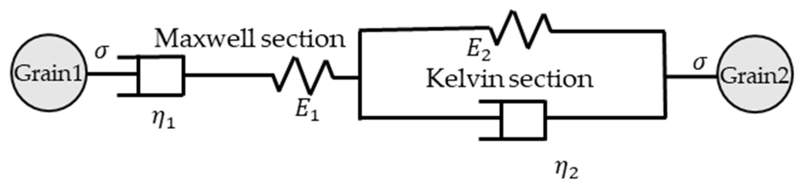
Burger’s model is composed of four mechanical components, including the series connection of the Newton dashpot and spring in the Maxwell section and the parallel connection of the Newton dashpot and spring in the Kelvin section (see Figure 3). The normal and tangential creep force between grains can be calculated after applying Burger’s model in the contacts. The constitutive equations involved in the calculation process is shown in

Table 1. The equations of Burger’s model and its components.

Model	Constitutive Equation [10]	Creep Equation
Maxwell model	$\sigma =E_1{\epsilon }_k+{\eta }_1\dot{{\epsilon }_k}$	$\epsilon =\frac{{\sigma }_0}{E_1}\left(1-\exp \left(-\frac{E_1}{{\eta }_1}t\right)\right)$
Kelvin model	$\dot{{\epsilon }_M}=\frac{\dot{\sigma }}{E_2}+\frac{\sigma }{{\eta }_2}$	${\epsilon }_M=\frac{1}{{\eta }_2}{\sigma }_{0}t+\frac{{\sigma }_0}{E_2}$
Burger’s model	$\ddot{\sigma }+\left(\frac{E_2}{{\eta }_1}+\frac{E_2}{{\eta }_2}+\frac{E_1}{{\eta }_1}\right)\dot{\sigma }+$ $\frac{E_1}{{\eta }_1}\frac{E_2}{{\eta }_2}\sigma =E_0\ddot{\epsilon }+\frac{E_1{E}_2}{{\eta }_1}\dot{\epsilon }$	$\epsilon =\frac{{\sigma }_0}{E_2}+\frac{\sigma }{{\eta }_2}t+\frac{{\sigma }_0}{E_1}\left(1-e^{-\frac{E_1}{{\eta }_1}t}\right)$

. The derivation of the creep equation only needs to apply a constant stress ${\sigma }_0$ at the initial time ($t_0$) in constitutive equations.

Figure 4 shows the components of the Parallel Bonded model and its strength criterion. The Parallel Bonded model consists of two pairs of springs with normal and tangential stiffness.

We can find that there are two kinds of special elements in Figure 4a, the bonded parts that are embedded in two branches of the structure and the separated sheets that represent the linear part of this model. One kind of the springs only produce the linear elastic force with normal and tangential stiffness, which ensures the linear elastic mechanical properties of the contact part. Another kind of spring has special components that can be broken under an ultimate load. Under normal circumstances, the Parallel Bonded model cements the grains to be rock-like and the grains can resist slide and rotation. If the Bonded parts are broken in an ultimate force, the corresponding structure will lose its function. The separated sheets can only resist compression force. Therefore, once the bonded part is broken, this model is deteriorated. From Figure 4b, we can analyze the broken criterion of PBM in PFC software. The applied force can be decomposed along the normal and shear direction of the contact surface. The force in the normal direction is termed $\sigma$ and the force in the shear direction is termed $\tau$. When the tension force in the normal direction is greater than ${\sigma }_c$, the bonded part will be broken and deteriorate into the linear elastic model. Similarly, the PBM will also be damaged if the shear force is greater than ${\tau }_c$. The symbols $\varphi$ and $c$ are the friction angel and cohesion coefficient of PBM. The shear force can be expressed as $\tau =c+\sigma \tan \varphi$.

According to Figure 3 and Figure 4, Burger’s model and the Parallel Bonded model can be regarded as physical models. They are all composed of explicit mechanical components, and it is convenient to combine them in series or parallel to derive a new model.

2.3. Analysis of Burger’s Bonded Model

In Section 2.1, we have simplified the mixed state and derived a model named Burger’s Bonded model in this paper.

Figure 5 shows the structure and components of Burger’s Bonded model. Burger’s Bonded model is equivalent to a five-parameter model in mechanics. $E_3$ in Figure 5 presents the total elastic stiffness of PBM. The property of parallel structure is that the two branches have the same displacement, and the stress is composed of the sum of the two forces in Burger’s part and the PBM part. Based on this feature, the constitutive model and creep equation can be derived.

For ease of analysis, the constitutive equation of Burger’s model listed in Table 1 is converted to Equation (1):

$$\sigma +{\alpha }_1\dot{\sigma }+{\alpha }_2\ddot{\sigma }={\beta }_1\dot{\epsilon }+{\beta }_2\ddot{\epsilon }$$

(1)

where ${\alpha }_1$, ${\alpha }_2$, ${\beta }_1$, and ${\beta }_2$ are constant coefficients of Burger’s model, the expressions of which are shown in Equations (4) and (5):

$${\alpha }_1=\frac{{\eta }_1+{\eta }_2}{E_1}+\frac{{\eta }_2}{E_2}$$

(2)

$${\alpha }_2=\frac{{\eta }_1{\eta }_2}{E_1{E}_2}$$

(3)

$${\beta }_1={\eta }_2$$

(4)

$${\beta }_2=\frac{{\eta }_1{\eta }_2}{E_1}$$

(5)

The coefficients ${\eta }_1$ and ${\eta }_2$ are the viscosity of the dashpots in Burger’s model (Maxwell section and Kelvin section, respectively), and the coefficients $E_1$ and $E_2$ are the elastic stiffness of springs in Burger’s model (see Figure 5).

In the parallel structure, the value of total stress equals the sum of two parallel branches, and the total strain is equal in two parts. Therefore, Equations (6) and (7) are obtained according to the stress and strain relationship, where ${\epsilon }_3$ and ${\sigma }_3$ are the strain and stress of spring $E_3$, and ${\epsilon }_c$ and ${\sigma }_c$ represents the strain and stress of Burger’s Bonded model, respectively. Note that $E_3$ represents the total elastic stiffness in the Parallel Bonded model part.

$${\epsilon }_c=\epsilon ={\epsilon }_3$$

(6)

$${\sigma }_c={\sigma }_3+\sigma$$

(7)

$${\sigma }_3=E_3{\epsilon }_3$$

(8)

Constitutive equations of Burger’s Bonded model (9) are obtained after submitting Equations (6)–(8) into Equation (1).

$${\sigma }_c+{\alpha }_1\dot{{\sigma }_c}+{\alpha }_2\ddot{{\sigma }_c}=E_3{\epsilon }_3+\left({\beta }_1+{\alpha }_1{E}_3\right)\dot{{\epsilon }_3}+\left({\beta }_2+{\alpha }_2{E}_3\right)\ddot{{\epsilon }_3}$$

(9)

According to the definition of creep, the strain behavior under a constant stress, and applying a constant stress ${\sigma }_0$ at $t=0$, Equation (10) can be obtained:

$$\ddot{{\epsilon }_c}+\left(\frac{{\beta }_1+{\alpha }_1{E}_3}{{\beta }_2+{\alpha }_2{E}_3}\right)\dot{{\epsilon }_3}+\left(\frac{E_3}{{\beta }_2+{\alpha }_2{E}_3}\right){\epsilon }_c-\frac{{\sigma }_0}{{\beta }_2+{\alpha }_2{E}_3}=0$$

(10)

To solve the differential Equation (10), the initial conditions should be considered. When $t=0$, the initial strain and initial stress, as well as initial viscosity conditions, are shown in Equations (11)–(13). After submitting Equations (11)–(13) into Equation (14), a new viscosity Equation (15) is derived.

$${\epsilon }_c=\frac{\sigma }{E_1}=\frac{{\sigma }_3}{E_3}$$

(11)

$${\sigma }_0={\sigma }_3+\sigma$$

(12)

$${\epsilon }_c=\frac{{\sigma }_0}{E_1+E_3}$$

(13)

$$\dot{{\epsilon }_c}=\frac{\sigma }{{\eta }_1}+\frac{\sigma }{{\eta }_2}$$

(14)

$$\dot{{\epsilon }_c}=\frac{\left({\eta }_1+{\eta }_2\right)E_1{\sigma }_0}{\left(E_1+E_3\right){\eta }_1{\eta }_2}$$

(15)

For ease of solving, the differential Equation (10) is simplified as Equation (16), where A, B, and C are constant material coefficients related to the model itself.

$$\ddot{{\epsilon }_c}+A\dot{{\epsilon }_c}+B{\epsilon }_c=C$$

(16)

For solving the differential equation, the root of the characteristic equation of the second-order nonhomogeneous linear system (16) is ${\lambda }_{1,2}$ and is shown in Equations (17) and (18). The general solution of the creep equation is expressed as Equation (17). To obtain a specific solution, the initial conditions need to be considered. After submitting Equations (12) and (13) into Equation (15), $C_1$ and $C_2$ are obtained.

$${\epsilon }_c=C_1{e}^{{\lambda }_{1}t}+C_2{e}^{{\lambda }_{2}t}+\frac{{\sigma }_0}{E_3}$$

(17)

$${\lambda }_{1,2}=-\frac{1}{2}\left[\frac{\left({\eta }_1+{\eta }_2\right)E_1{E}_3}{\left(E_1+E_3\right){\eta }_1{\eta }_2}+\frac{E_1}{{\eta }_1}\right]\pm \frac{1}{2}\sqrt{{\left[\frac{\left({\eta }_1+{\eta }_2\right)E_1{E}_3}{\left(E_1+E_3\right){\eta }_1{\eta }_2}\right]}^2-4\frac{E_1{E}_2{E}_3}{{\eta }_1{\eta }_2\left(E_1+E_3\right)}}$$

(18)

$$C_1=\frac{\left({\eta }_1+{\eta }_2\right)E_1{E}_3{\sigma }_0+{\lambda }_2{E}_1{\eta }_1{\eta }_2{\sigma }_0}{\left({\lambda }_1-{\lambda }_2\right)\left(E_1+E_3\right){\eta }_1{\eta }_2{E}_3}$$

(19)

$$C_2=\frac{\left({\eta }_1+{\eta }_2\right)E_1{E}_3{\sigma }_0+{\lambda }_1{E}_1{\eta }_1{\eta }_2{\sigma }_0}{\left({\lambda }_2-{\lambda }_1\right)\left(E_1+E_3\right){\eta }_1{\eta }_2{E}_3}$$

(20)

Similarly, when unloading happens at a certain time $t_0$, the analytical solution of the elastic hysteresis equation can be analyzed. Applying ${\sigma }_c=0$ to Equation (9), Equation (21) is derived, and the general solution form of the homogeneous linear differential equation is expressed as Equation (22).

$$E_3{\epsilon }_c+\left({\beta }_1+{\alpha }_1{E}_3\right)\dot{{\epsilon }_c}+\left({\beta }_2+{\alpha }_2{E}_3\right)\ddot{{\epsilon }_c}=0$$

(21)

$${\epsilon }_c=D_1{e}^{{\lambda }_{1}t}+D_2{e}^{{\lambda }_{2}t}$$

(22)

To obtain the value of $D_1$ and $D_2$, we need to submit the initial conditions (Equations (23)–(26)) into Equation (22), and the expression of $D_1$ and $D_2$ is obtained shown in Equations (27) and (28):

$${\epsilon }_0=D_1{e}^{{\lambda }_1{t}_0}+D_2{e}^{{\lambda }_2{t}_0}$$

(23)

$$\dot{{\epsilon }_0}=D_1{\lambda }_1{e}^{{\lambda }_1{t}_0}+D_2{\lambda }_2{e}^{{\lambda }_2{t}_0}$$

(24)

$${\epsilon }_0=C_1{e}^{{\lambda }_1{t}_0}+C_2{e}^{{\lambda }_2{t}_0}+\frac{{\sigma }_0}{E_3}$$

(25)

$$\dot{{\epsilon }_0}=C_1{\lambda }_1{e}^{{\lambda }_1{t}_0}+C_2{\lambda }_2{e}^{{\lambda }_2{t}_0}+\frac{{\sigma }_0}{E_3}$$

(26)

$$D_1=C_1+\frac{{\sigma }_0{\lambda }_2}{E_3\left({\lambda }_2-{\lambda }_1\right)e^{{\lambda }_1{t}_0}}$$

(27)

$$D_2=C_2+\frac{{\sigma }_0{\lambda }_1}{E_3\left({\lambda }_1-{\lambda }_2\right)e^{{\lambda }_2{t}_1}}$$

(28)

This paper has given the constitutive model of Burger’s Bonded model in Figure 3, the constitutive equation in Equation (9), the creep equation in Equation (17), and the elastic hysteresis equation in Equation (22). In the next section, the influence of the model’s parameters on the rheological properties will be analyzed. Note that the rheological properties (time-dependent properties) include creep and elastic hysteresis. Although the elastic hysteresis properties are not the point of this article, it will also be useful to the research of soft-rock time-dependent mechanical behavior and be convenient in the use of Burger’s Bonded model.

2.4. The Influence of Model Parameters on Deformation Behavior

To further study the five parameters in BBM analytical equations, we try to obtain the deformation curves by assigning different parameter values (see

Table 2. ${\eta }_1$ as variable.

${\mathit{\eta }}_1$$/{10}^4$	${\mathit{\eta }}_2$$/{10}^5$	${\mathit{E}}_1$$/{10}^7$	${\mathit{E}}_2$$/{10}^7$	${\mathit{E}}_3$$/{10}^7$
2	6	1	1	1
6
10

,

Table 3. ${\eta }_2$ as variable.

${\mathit{\eta }}_1$$/{10}^4$	${\mathit{\eta }}_2$$/{10}^5$	${\mathit{E}}_1$$/{10}^7$	${\mathit{E}}_2$$/{10}^7$	${\mathit{E}}_3$$/{10}^7$
6	2	1	1	1
	6
	10

,

Table 4. $E_1$ as variable.

${\mathit{\eta }}_1$$/{10}^4$	${\mathit{\eta }}_2$$/{10}^5$	${\mathit{E}}_1$$/{10}^7$	${\mathit{E}}_2$$/{10}^7$	${\mathit{E}}_3$$/{10}^7$
6	6	0.5	1	1
		1
		1.5

,

Table 5. $E_2$ as variable.

${\mathit{\eta }}_1$$/{10}^4$	${\mathit{\eta }}_2$$/{10}^5$	${\mathit{E}}_1$$/{10}^7$	${\mathit{E}}_2$$/{10}^7$	${\mathit{E}}_3$$/{10}^7$
6	6	1	0.5	1
			1
			1.5

and

Table 6. $E_3$ as variable.

${\mathit{\eta }}_1$$/{10}^4$	${\mathit{\eta }}_2$$/{10}^5$	${\mathit{E}}_1$$/{10}^7$	${\mathit{E}}_2$$/{10}^7$	${\mathit{E}}_3$$/{10}^7$
6	6	1	1	0.5
				1
				1.5

).

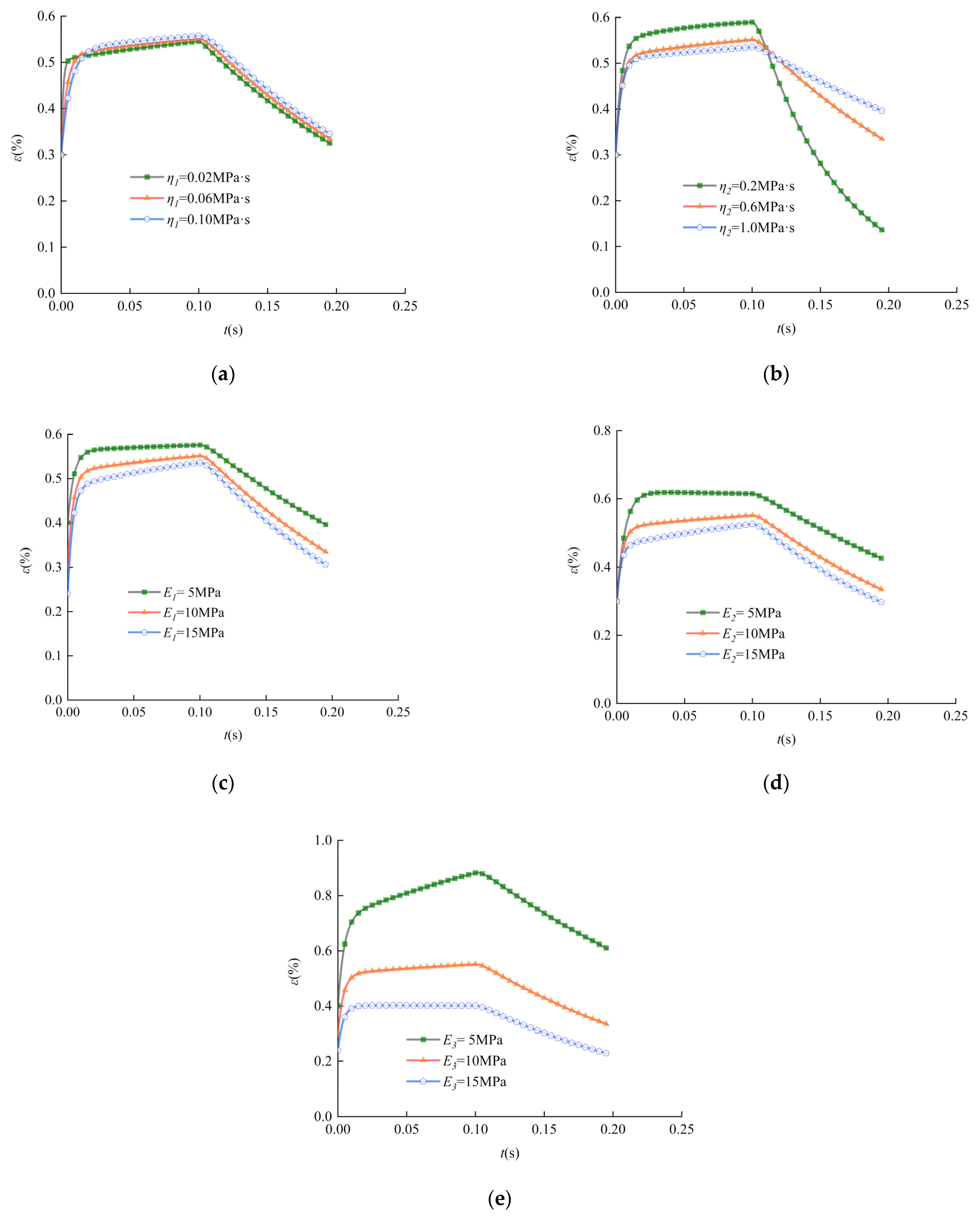
These curves are derived from the algebra calculation with Equations (17) and (22). We apply the stress ${\sigma }_0$ = 6 MPa into Equation (17), then we set the timestep interval as 0.001 s to obtain a series of calculation results about $\epsilon$. After 100-times calculation, the creep curves are shown in Figure 6 (before 0.1 s). Then the unloading curves are also derived from Equation (22) after t = 0.1 s, and the timestep interval is also set as 0.001 s. Then we can obtain a series of calculation results about ε in the unloading process.

Note that this process is qualitative research. Since ${\eta }_2$ is the series part of the Maxwell section, its value is critical to attenuated creep performance, so the value is deliberately enlarged to obtain a better attenuated creep curve visually. The creep curves and elastic hysteresis curves are shown in Figure 6.

The values ${\eta }_1$ and ${\eta }_2$ represent the viscosity coefficients of dashpots in Burger’s Bonded model. Figure 6a shows that a larger value of ${\eta }_1$ will result in a quicker decreasing rate of attenuated creep but has little effect on the steady creep. Figure 6b shows that the starting point of steady creep and the elastic hysteresis rate will decrease with the increase of ${\eta }_2$.

The values $E_1$ and $E_2$ represent the stiffness of springs in Burger’s Bonded model. From Figure 6c, it can be found that increasing the value of $E_1$ has no significant effect on the attenuation rate and elastic hysteresis rate but will decrease the initial elastic deformation of attenuated creep and will increase the steady creep rate. According to Figure 6d, increasing the value of $E_2$ has little impact on the attenuated creep and the rate of elastic hysteresis, but will reduce the starting point of steady creep and increase the steady creep rate. The value $E_3$ represents the stiffness of the Parallel Bonded parts. Figure 6e shows that the initial elastic deformation and the attenuating rate will decrease with the increase of $E_3$. Moreover, it will reduce the starting points and the rates of steady creep and slow down the decay rate of attenuated creep and the rate of elastic hysteresis.

The results have shown that the value of $E_3$ has a significant effect on the mechanical behavior of Burger’s Bonded model, and the other four parameters will serve as a modifying effect. This phenomenon is mainly caused by the parallel structure. $E_3$ acts as an integral branch, but the others jointly make up a branch.

Burger’s Bonded model’s parameters with different values will affect the performance of creep curves. Because the DEM is based on the mechanical behavior of discrete particles, the constitutive relationship of particle assemblies is also dependent on the micro-mechanical parameters of particles and their contacts. In general, the calibration process can be divided into two steps. The first step is carrying out experiments and obtaining mechanical properties of rock. The second step is choosing and modifying the micro-parameters of DEM, which is time consuming and complicated. The study in this section will be helpful in the calibration process of DEM simulation, which can greatly reduce the ‘trial and error’ time.

2.5. The DEM Model Parameters’ Assignment

Normally, the basic mechanical properties of soft rock can be reflected by loading tests and the time-dependent properties can be reflected by creep tests. Therefore, we designed the loading test and creep test in DEM to verify the reliability of the improved method in this paper. The DEM model generation method has been introduced in Section 2.2.

To the convenience of the analysis of results, the parameters’ calibration process is dependent on the published experimental results from Zhou et al. [32]. The experimental materials are typical soft rocks in South China, and the sample size is 50 × 50 × 100 mm in a cuboid. The process of the creep test is gradually loading from 2 MPa to 10 MPa in five stages, and the loading time of each stage remains 24 h. In the loading test, the twist drill was used to prefabricate 10 mm × 25 mm cracks with different angles (15°, 45°, and 80°, respectively). Then, the test process continued to load the specimen at a rate of 0.04 mm/min until it was destroyed. The whole test process was carried out in the TAW soft rock test system developed by Sun Yat-sen University.

The DEM model’s parameters are shown in

Table 7. The value of parameters in the DEM model.

Radius/mm	${\mathit{E}}_3/\mathbf{GPa}$	${\mathit{\sigma }}_{\mathit{c}}/\mathbf{MPa}$	c/MPa	$\mathit{\phi }$/(°)	${\mathit{E}}_1/\mathbf{GPa}$	${\mathit{E}}_2/\mathbf{GPa}$	${\mathit{\eta }}_2/{10}^7$	${\mathit{\eta }}_1/{10}^7$	Porosity/%	Density/Kg/m3
0.2–0.5	1.45	30	11	30	0.1	0.1	1	0.1	0.16	2600

, which is calibrated carefully depending on experiments. The size of the two-dimensional DEM model needs to be determined as 50 mm × 100 mm, which is consistent with the experiments. Note that the grain size in DEM is not the same as the actual physical size for the reason of calculating efficiency. As the particle scale is magnified, the simulation effect can also be guaranteed. In DEM simulation, the strength and elastic modulus of the model will increase with the model length to grain radius (L/d), but this increase rate will be much smaller when L/d is greater than 40 [33,34]. Therefore, the particle radius is applied at 0.2~ 0.5 mm in this paper, which not only meets the accuracy requirement but also considers the computational efficiency. The DEM model’s strength depends on $c$ and ${\sigma }_c$ parameters, and this calibration process adopts the method shown in reference [35]. The value assignment of $E_1, E_2,E_3, {\eta }_1, {\eta }_2$, and other parameters is listed in Table 7 too, which is calibrated by the experiments and the law shown in Figure 6. In addition, this paper uses the Smooth Joint model to simulate cracks, which is used widely in mimicking crack behavior in DEM [36]. Note that the DEM creep simulation is calculated 10 million times at each stage to ensure a long steady creep and the rate of uniaxial loading test is the same as experiments. The value of the timestep is affected by the system stiffness and calculation stability. In our simulation process, the timestep is applied as a $4\times {10}^{-8}$ s/step.

3. Results

Two kinds of DEM simulations are compared with experimental results, and some mechanical mechanisms are analyzed based on DEM mesoscopic phenomena in this section.

According to the basic knowledge of creep in soft rock, many researchers have revealed that the grain’s dislocation mechanism and the bond’s failure mechanism will cause creep in actual experiments. Therefore, based on the meso-mechanical property of DEM, we can analyze both of the abovementioned creep mechanisms.

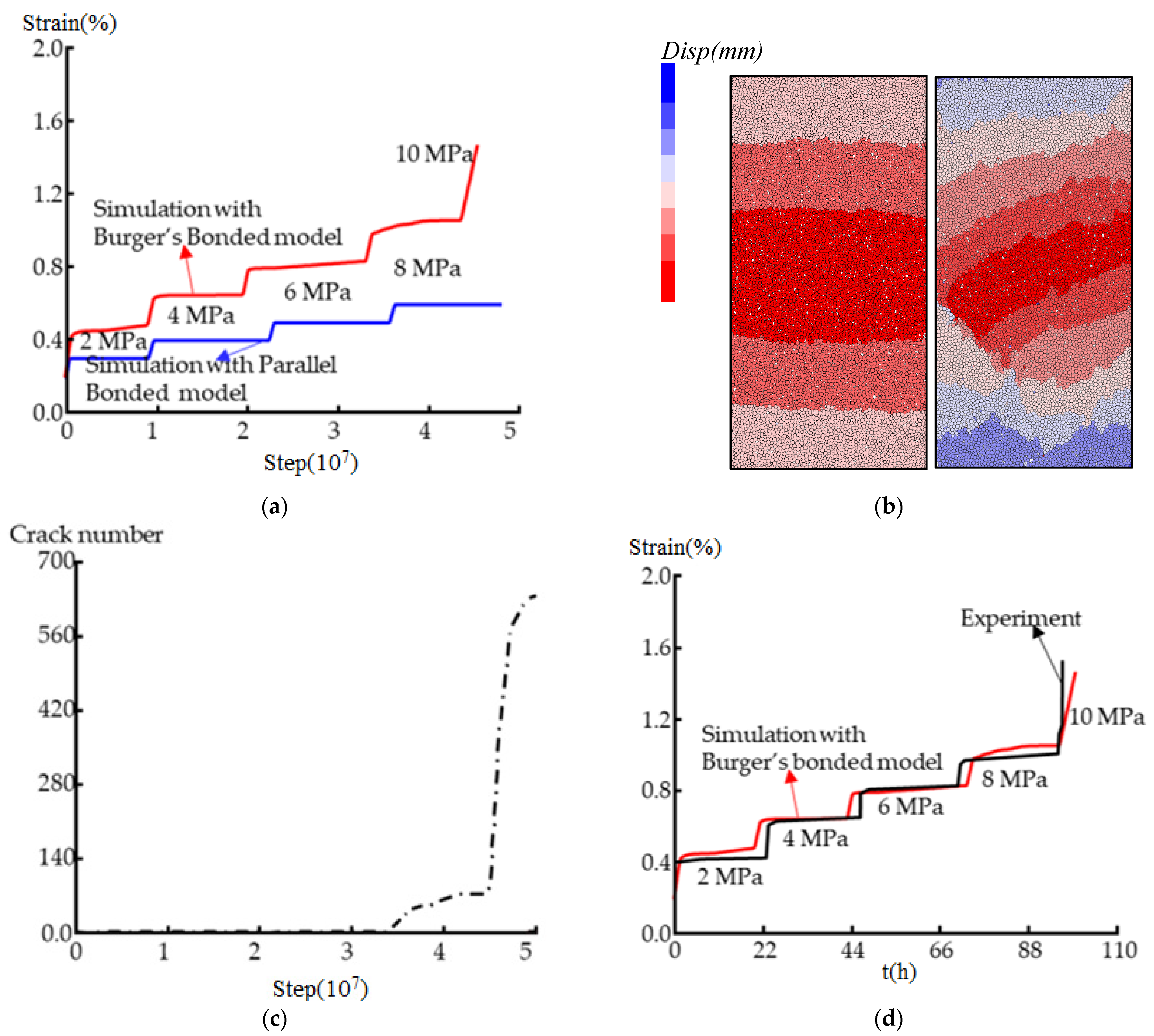
Firstly, according to Figure 7a, we find that the classic PBM cannot be used to simulate the creep behavior. In different loading stages, the strain will not change with time in the simulation process, which is weak in reflecting soft rock’s mechanical behavior. By contrast, the new simulation method adopting the BBM model can reflect the creep behavior of soft rock. In Figure 7b, we can find the grain’s dislocation phenomenon in BBM, which cannot be found in PBM. The following reasons may account for this: (1) The PBM causes the grains assembly to be a rigid rock-like material, which will not cause tiny dislocation in grains before the damage stage. (2) The BBM model has added many creep elements (Burger’s model) into the specimen, which is not connected by the cementation effect, therefore under loading, the dislocation process will gradually appear and cause the creep behavior in the initial stages. In Section 2.1, we have explained that the full stage creep can be divided into attenuated, steady, and accelerated creep. The dislocation-induced creep behavior can reflect the creep deformation in early stage. From Figure 7c, we can further study the damage mechanism caused by creep in the accelerated stage. Note that the crack information is recorded in the mixed model (BBM), and only the PBM in the mixed model can be broken under stress. From the perspective of the micro-crack’s propagation, we can easily find that the damage will not appear in attenuated creep and the steady creep stage. The irreversible damage finally causes the accelerated creep when the 10 MPa axial stress is applied to the specimen. Additionally, we can compare the creep curves between numerical tests and actual experiments. Figure 7d shows the errors of the calibrated simulation results. We can find that the general creep behavior in different stages can be revealed, including the attenuated and steady creep before 8 MPa loading and the accelerated creep in 10 MPa loading. There are some minor discrepancies in the curves: (1) The simulation result shows a larger creep deformation in the first 2 MPa loading process, which can be explained by the initial pores compaction stage leading to the variation of elastic modulus in the actual experiment, which is hard to simulate in the DEM. (2) The fourth stage of simulation results also shows larger deformation than the experiment, which is caused by the complicated damage process in the actual experiment, and this is simplified in the DEM simulation process. In general, the simulation results can reveal the full-stage creep process of the soft rock and can also reveal the multi-factor-caused creep mechanism.

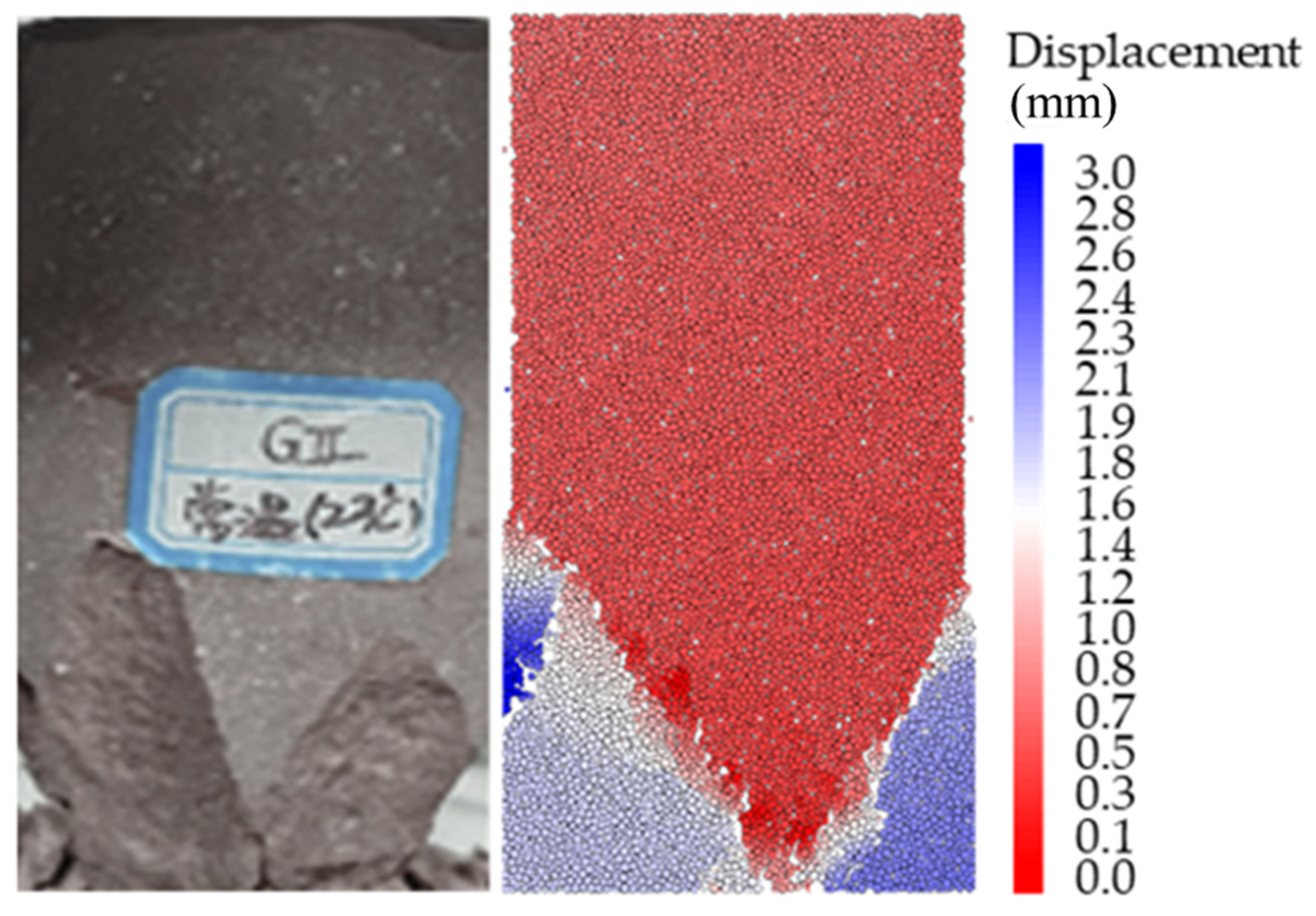
Figure 8 The damaged specimen shows a conical shape with some wing cracks. We can find that there is no obvious integral crack in these samples, which means the creep-induced failure is not caused by dramatic energy release. The gradually accumulated large deformation finally leads to this kind of failure pattern. Meanwhile, we can find that the simulation results in the creep test is consistent with the experiment.

We have described the simulation method proposed in this article and its creep behavior simulation effect. However, if the simulation ability is limited at the creep simulation, this method loses its meaning. We want to prove that the improved simulation method in this paper can simulate the complicated creep behavior of soft rock, which is not under the price of losing its capacity in the loading mechanism. Herein, we also adopt the same numerical specimen used in creep tests.

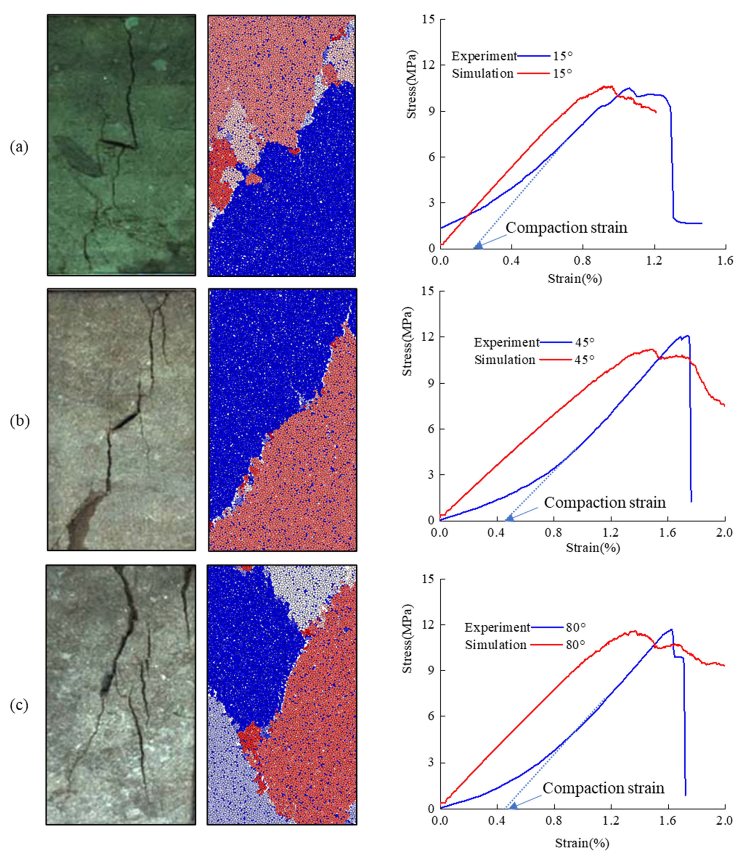
Figure 9 shows the results of uniaxial loading tests in DEM and the comparison with experiments. In the verification process, we want to describe the compaction stage that appears in the early loading stage of soft rock. In the natural state, the soft rock is a porous medium, which will experience an obvious pore space compaction stage. This process will cause an obvious stiffness variation in the stress–strain curves. However, in the DEM simulation, the grains are completely rigid and cannot simulate this compaction stage. Under the abovementioned description, we can analyze the stress–strain curves. From Figure 9, we can find that in the pre-peak stages, three specimens all show an obvious compaction stage and cause a strain discrepancy with the numerical results. In the numerical research process, we mainly consider the elastic modulus (the slope of the stress–strain curve) in the linear stage and the peak strength. From the strength and linear elastic modulus aspect, the simulation results are acceptable. Yet, there are some discrepancies in the post-peak stage of stress–strain curves. To explain this point, we need to know the actual experimental process in a loading machine. When the loading is applied to the rock, the deformation and strain energy stored in the machine will be released dramatically and effect the full-stage stress–strain recording in the post-peak stage. Therefore, we can find the stress drop phenomena in Figure 9b,c. However, in the DEM simulation process, the loading process is applied in a strict deformation control, which will not cause the stress drop in the post-peak stage.

Despite the discrepancies in the compaction stage and post-peak stage, the BBM in this paper can reflect the basic stress–strain curves in the loading process. In addition, we can analyze the damage propagation process combining Figure 9 and Figure 10. In Figure 9, we have shown three final states of pre-cracked samples and the numerical results. We can find two phenomena in Figure 9: (1) The crack angle is near 90° in the experiment and 60° in the numerical result. (2) Except for some wing cracks and the difference in angle, the crack shapes in the numerical results are similar to the experiments. 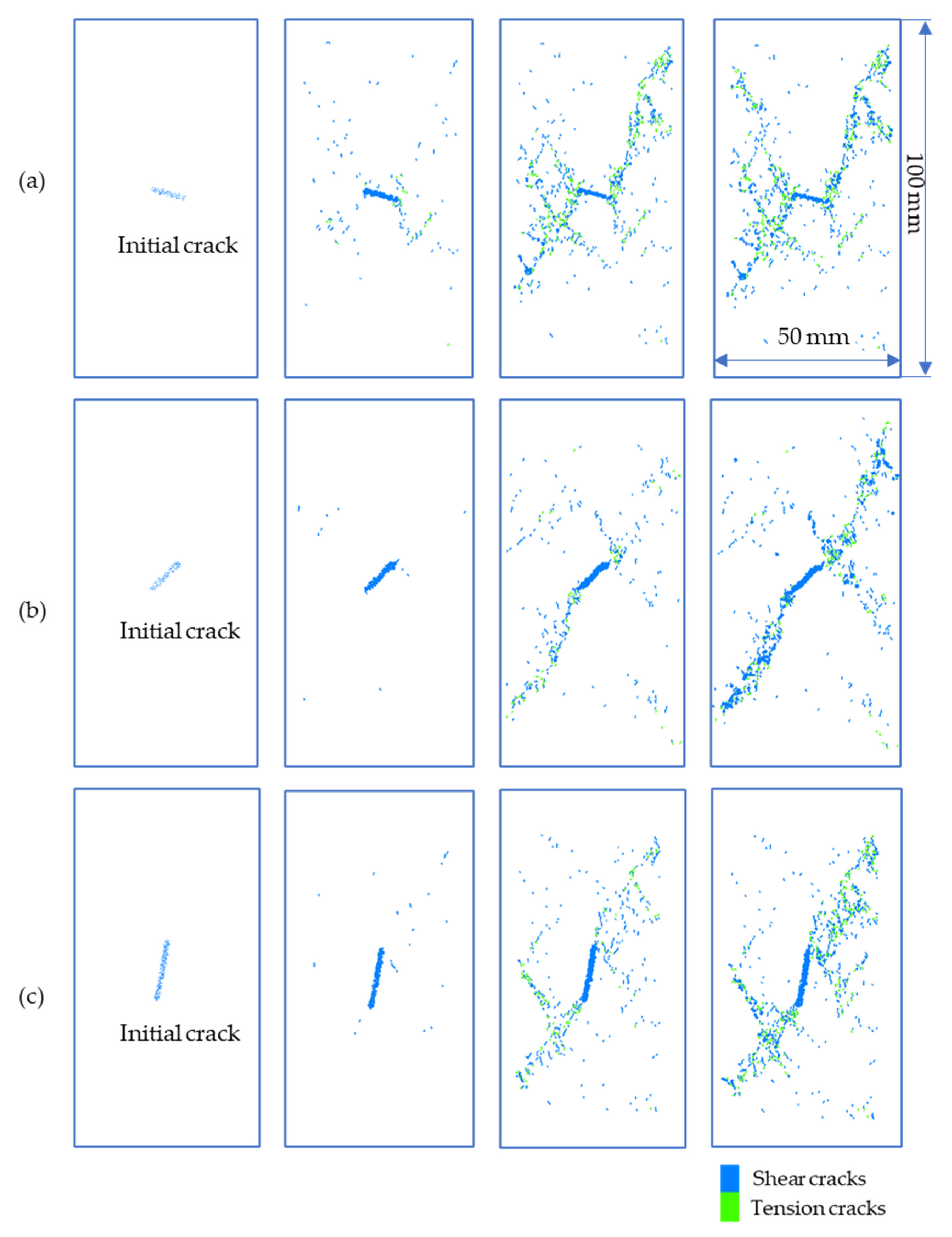From Figure 10, we can firstly analyze the micro-crack propagation process. Note that there are two kinds of cracks in DEM system. In Section 2.1, we have explained the PBM failure criterion, whereby if the bond is damaged by shear force, then one shear crack is recorded. Similarly, if the bond is damaged by tension force, the tension crack will also be recorded. The micro-crack gradually developed in different loading stages, and we captured the crack information during the stress-increasing process. The first stage is the initial stage where we can find three pre-cracks in the samples. The different angle of the initial cracks may have an impact on the damage propagation process. Yet, we cannot find the relation between the initial cracks and damage propagation in the second stage of all specimens. In the second stage, the new developed micro-cracks are distributed randomly. Then, in the third stage, the micro-cracks have fully developed and clustered along a 60° degree from horizontal direction. Until now, we can explain why the final cracks in Figure 9 are near 60°. This phenomenon is caused by the internal property of soft rock, which is slightly affected by the pre-cracks. Therefore, the experiments and numerical results all show similar law of the final cracks. What is more, we can find that the shear cracks and tension cracks are distributed in the final stage. The amount of tension cracking is greater than shear cracking, which means most of the bonds are damaged by the tension force in the local area.

In general, the linear elastic modulus, peak strength, and basic crack conditions can be simulated by the improved simulation method in this paper. We know there are some errors in simulation process, but the numerical method is a simplified way to reflect complicated problems. From this perspective, the simulation method proposed in this paper can mimic the mechanical process of soft rock under loading conditions especially for time-dependent properties.

4. Conclusions

A new simulation method for soft rock mechanical behaviors based on Burger’s model and the Parallel Bonded model is proposed. A simplified model named Burger’s Bonded model in the simulation process is derived and the analytical analysis is completed. The following conclusions are drawn:

• The improved method proposed in this paper can simulate the full-stage creep characteristics of soft rock and is consistent with experiments, which has considered the creep caused by grain dislocation and bonds damage mechanism. This method can also qualitatively describe the crack development and the stress–strain of soft rock in loading.
• The simplified model is a physical creep constitutive model, which has combined the properties of Burger’s model and the Parallel Bonded model. This model builds a bridge between the classic creep model and DEM simulation.
• A series of analytical equations are given. The research on the parameters’ effect on rheological behavior can be applied to the DEM calibration process and also has potential in engineering design.