Predicted Mapping of Seabed Sediments Based on MBES Backscatter and Bathymetric Data: A Case Study in Joseph Bonaparte Gulf, Australia, Using Random Forest Decision Tree

Abstract

Predictive mapping of seabed sediments based on multibeam bathymetric (BM), and backscatter (BS) data is effective for mapping the spatial distribution of the substrate. A robust modeling technique, the random forest decision tree (RFDT), was used to predict the seabed sediments in an area of the Joseph Bonaparte Gulf, Northern Australia, using the multibeam data and seabed sediment samples collected simultaneously. The results showed that: (1) Using multibeam bathymetry data in addition to multibeam backscatter data improves the prediction performance of the RFDT. In comparison to only multibeam backscatter data, the prediction performance achieved a ~10% improvement in sediment properties; it achieved a ~44.45% improvement of overall accuracy in sediment types, and a ~0.55 improvement in Kappa. (2) The underlying relationships between sediment properties and multibeam data show that there is an opposite non-linear correlation between sediment property-BS and sediment property-BM. For example, there is an obvious negative relationship between %mud-BS at incidence angles of 13° and 21°, but the relationship between %mud-BM is positive. As such, the RFDT is a useful and well-performing method in predicting the relationship between sediment properties and multibeam data and in predicting the distribution of sediment properties and types. However, the sediment prediction method in deep-water areas with high gravel content needs to be further evaluated.

1. Introduction

Seabed sediments are an important seabed interface as accurate seabed characteristics over a large area are significant in mapping benthic habitats [1,2,3,4,5], identifying seabed geological environment [6,7,8,9,10], and managing marine protected areas [11]. The traditional in situ sampling method of seabed sediments is not suitable for the mapping of a large area of seabed substrate because of its disadvantages such as a limited number of samples, high sampling cost, and low reliability. In contrast, the rapid development of acoustic remote sensing techniques that utilize the emission and return of acoustic signals to describe seafloor morphology and seabed texture has played an increasingly important role in the mapping of the seabed environment. In particular, the modern multibeam echo-sounder system (MBES) is capable of collecting multibeam bathymetry (BM) and backscatter (BS) data simultaneously from hundreds of narrow-angle beams that create small footprints on the seabed.

Many studies have shown that acoustic BS has a strong correlation with sediment properties [12,13,14,15,16]. Although the relationships between sediment properties and BS are often not linear, they generally show that coarser sediment is associated with a stronger backscatter intensity return than finer sediment [13,16,17,18,19]. For example, previous studies have shown that BS has a positive correlation with sediment mean grain size (MGS) [12,15,20,21,22]. This backscatter-sediment relationship thus forms the foundation for using BS for seabed sediment mapping [2,10,23,24,25,26,27]. In addition, previous studies have demonstrated that the angular response of the BS can improve the overall accuracy of the predicted classes. [9,23,24,28,29,30,31,32]. Various methods have been used for automatic classification and mapping, including decision trees (DT) [30,33,34,35,36], random forest decision tree (RFDT) [37,38,39,40,41], support vector machines (SVM) [42,43], artificial neural networks (ANN) [44], QTC Multiview [26,27], clustering [45] and maximum likelihood classifier (MLC) [35,43]. Of these methods, the RFTD, which uses the bagging process for performance evaluation [37], is used to directly obtain the overall prediction accuracy. Approximately two-thirds of the samples (in-bag samples) were randomly selected for tree construction, and the remaining one-thirds of the samples (out-of-bag samples, OOB) were used for error evaluation. At the same time, OOB samples are also used to estimate the relative importance of explanatory variables [31,37,46]. Moreover, retests can be performed using the explanatory variables with higher relative importance to improve the prediction accuracy of the model [41]. Previous studies have shown that sediment samples were obtained by sampling in a single region [31,41], which inevitably led to limitations in sample types. In the supervised classification process, the acoustic class is directly related to the true ground types. Whether the acoustic type of the supervised classification is consistent with the true substrate type of the sample area remains to be studied.

In this study, we used the RFTD to rank the importance of explanatory variables. Relatively important variables were selected to explore the correlation between acoustic signals (multibeam BM and BS) and sediment attributes, thereby classifying and mapping the sediment types. We also examined whether additional BM and its derivatives would improve the prediction performance of sediment mapping. The ultimate aim was to predicatively map a large area of the seabed substrate predicatively by applying the RFDT. The flow chart of the data processing and analysis in this study is shown in Figure 1.

2. Study Area and Data

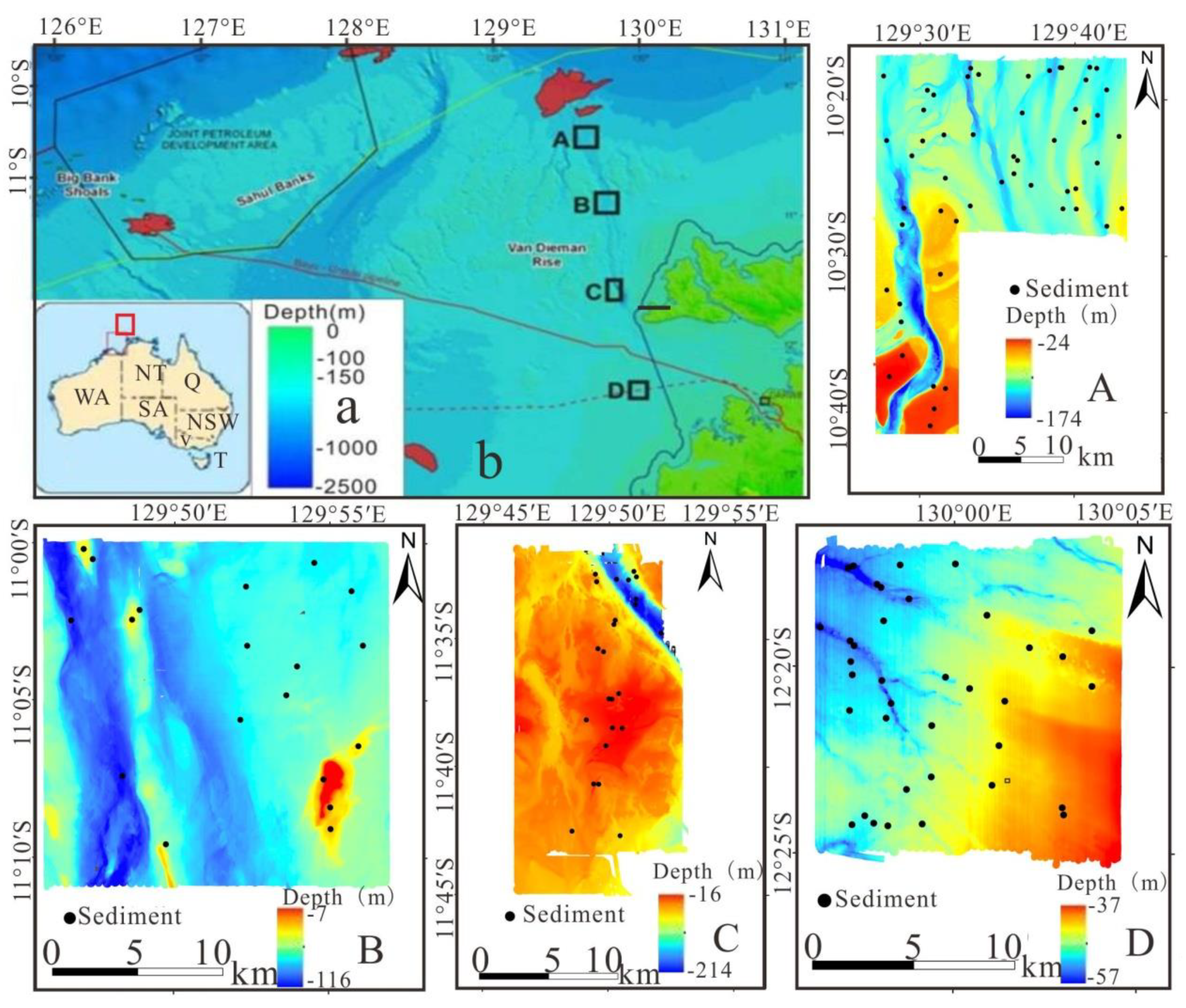
2.1. Study Area

The Joseph Bonaparte Gulf is located at Northern Australian margin (Figure 2a), and the multibeam and sediment data were acquired in four areas by Geoscience Australia [47,48,49]. The seabed environments were extensive, shallow carbonate-dominated margins [47,48]. The banks and channels covered by the four areas could be considered as representative of the north Australian shelf (Figure 2b) [49]. The sediments in Joseph Bonaparte Gulf mainly originate from the multitudinous rivers in tropical region of Australia [50]. They are mainly composed of carbonate grains [47]. The sediments are dominated by muddy sands with well-sorted coarser to medium sands. In order to increase the diversity of the samples, we collected data from four sub-regions. They were located on the outer-shelf region, away from the coast to near-shore area with BM ranging from 24 to 174 m (BP_A, Figure 2A), 7 to 116 m (BP_B, Figure 2B), 16 to 214 m (BP_C, Figure 2C) and 37 to 57 m (BP_D, Figure 2D). The areas contain a variety of complex topography, including flat bed, deep valleys, and plains, etc. (Figure 2A–D). This made it easier for us to collect more types of ground true values. The data collected from the BP_A area were used in two experiments, one was that BM and BS were used as explanatory variables, the other was that only BS was used as explanatory variables. Based on the better performance of experiment, we pooled the data of four sub-regions (BP_A- D) to predict the distribution of acoustic classes.

2.2. Sediment Samples and Property

A total of 132 sediment samples were collected from the four areas at representative locations using Smith Macintyre grab (0.1 m²) in August and September 2009, and July and August 2010. They were analyzed in the laboratory to obtain four sediment properties. The properties of %sand, %mud and %gravel were obtained using the wet sieve separation method [51], and the MGS was obtained by the laser granulometry method (a Malvern Mastersizer 2000, Malvern Instruments Ltd., Worcestershire, UK). These sediment samples were also classified into sediment types according to the modified Folk classification scheme [52]. The 132 sediment samples are shown in

Table 1. The modified Folk classification for classifying the sediment samples.

Seabed Sample Types	Radio of Sand to Mud	%Gravel	Number of Samples
sandy Gravel (sG)	>9	30–80%	9
muddy sandy Gravel (msG)	1–9	30–80%	5
gravelly Sand (gS)	>9	5–30%	9
gravelly muddy Sand (gmS)	1–9	5–30%	59
Sand (S)	>9	<5%	6
muddy Sand (mS)	1–9	<5%	39
sandy Mud (sM)	<9	<5%	4

, while the samples of each sub-region are listed in

Table 2. The types and numbers of sediment samples in the four sub-regions.

	sG	msG	gS	gmS	S	mS	sM	Numbers
BP_A	5	1	4	14	4	26	--	54
BP_B	--	2	1	14	1	--	--	18
BP_C	4	2	3	7	1	3	3	23
BP_D	--	--	1	25	--	10	1	37
Numbers	9	5	9	60	6	39	4	132

.

2.3. Multibeam Data and Its Processing

Raw BM and BS were collected using a 300 kHz Kongsberg EM3002 MBES. For each survey, the MBSE was calibrated against a reference seabed to ensure the levels of the BS and BM were consistent. The reference seabed should be smooth, sandy and flat [53]. The multibeam data included the BM and its derivatives. BS was finally generated in ArcMap 10.2 as raster data with a resolution of 10 m × 10 m. The Smith-McIntyre grab had an opening of 0.1 m², which was smaller than the cell size of the multibeam data (100 m²). The sample locations were determined using the same DGPS system as the multibeam surveys, which were highly error-free in terms of horizontal accuracy.

2.3.1. Backscatter Data

The raw BS was processed in Geoscience Australia using the CMST-GA MB Process v8.11.02.1 software, which was co-developed by Geoscience Australia and the Center for Marine Science and Technology at Curtin University of Technology [54,55]. The post-processing included the corrections of acoustic signal loss during transmission, the influence of the ensonification area, and the removal of the system implemented model [54,55]. An along-track sliding window of 100 pings was used to calculate the mean angular response. We also removed the angular dependence to obtain BS mosaics normalized to select incidence angles and to obtain the real angular response curves of the BS [56,57,58]. Finally, the normalized backscatter at the incidence angle (BIA) between 1 and 60°, with an interval of 1°, was generated by the mean BS value within the window [59]. These 60 BS mosaics effectively form a BS angular response curves dataset [15,28,32]. The spatial resolution of these BS mosaics was set to 10 m for the Joseph Bonaparte Gulf, which was approximately 2% of the BM.

2.3.2. Bathymetric Data and Derivatives

The raw BM was processed using the Caris Hips and Sips V6.1 software. The calibrations included applying motion sensor information (e.g., differential GPS, roll, pitch and yaw), correcting tidal variations using the WXTide32 software (http://www.wxtide32.com, accessed on 1 January 2012), removing spikes and outliers, and correcting sound velocity variations. The corrected bathymetric data were generated as grid data of 10 m cell size. Several derivatives were derived from bathymetric data, including slope, benthic position index (BPI) [60], and surface area (SA) [61]. At the end of data processing, we reassembled all the explanations with Arcmap10.2 software with cell size of 10 m × 10 m. BPI refers to the difference between the elevation of the center point and the average of the surrounding elevations. The calculation formula is as follows:

$$\mathrm{BPI}=\mathrm{e}-{\displaystyle \sum }_{\mathrm{i}=1}^8{\mathrm{e}}_{\mathrm{i}}/8$$

(1)

where e is the elevation.

3. Sediment Mapping Methods

This study used a robust predictive modeling technique, RFDT, to map seabed sediments in the study area [37,40,41]. The modeling steps included the selection of target and explanatory variables, tuning of modeling parameters, searching for the best combination of explanatory variables, accuracy assessment, and generation of predictive relationship curves. The final models were then used to generate predictive maps of sediment types and properties.

3.1. Predictive Model—Random Forest Decision Tree

The RFDT technique was implemented using the DTREG software [37] (http://www.dtreg.com, accessed on 1 January 2021). It has the ability to model the nonlinear relationship between the target and explanatory variables and calculate the relative importance of the explanatory variables. The model uses the proportion of variance explained (R²) and overall accuracy as statistics to evaluate the prediction performance of sediment grain size properties and sediment types, respectively. In order to maximize the prediction accuracy of the models, the best combinations of explanatory variables were selected manually according to R² or overall accuracy (detailed in Section 3.1.3).

3.1.1. Target and Explanatory Variables

In this study, the explanatory variables contained BS mosaics at 45 incidence angles, BM, slope, surface area (SA), and BPI. The target variables are numerical variables of %gravel, %sand, %mud, and MGS, and a categorical variable of sediment types. Post raw BS data processing, it was noticed that there is missing data when the incidence angle is less than 5° and greater than 45°. Therefore, we selected the BS between 5 and 45° as the explanatory variables.

3.1.2. Selection of the Best Combination of Modeling Parameters

The first modeling step was to select the best combination of modeling parameters. The model parameters, the “number of trees in forest,” the “minimum size node to split” and the “maximum tree levels” have an important influence on the prediction accuracy of the random forest model. To optimize the modeling performance, we used all 45 explanatory variables to determine the best combination of model parameters with the highest R² or overall accuracy. The number of trees in this step was predetermined. The value was 200 when the samples were only from BP_A, and it was 1000 when the samples were from all four sub-regions. We only changed two parameters: the “minimum size node to split” parameter varied between 2, 3, 4, 5 and 6 and the “maximum tree levels” parameter varied between 5, 10, 15, 20, and 25. Therefore, in total there were 25 combinations of parameters that were tested in this step.

After a trial-and-error process, the parameters of RDFT were set as follows:

The samples were from BP_A:

• Number of trees in the forest: 200;
• Maximum tree levels: 10;
• Minimum size node to split: 3;
• Random predictor control: square root of total predictors and overall accuracy.

The samples were from BP_A-BP_D:

• Number of trees in the forest: 1000;
• Maximum tree levels: 10;
• Minimum size node to split: 4;
• Random predictor control: overall accuracy.

3.1.3. Selection of the Best Combination of Explanatory Variables

In this second step, we manually selected the best combination of explanatory variables to improve the overall prediction accuracy from the previous step; this was an interactive process. In the first iteration, we selected only one of the 45 explanatory variables that had the best prediction performance (e.g., the highest adjusted R² or overall accuracy). In the second iteration, the remaining explanatory variables were added to the model one by one; again, the variable with the best prediction performance was selected as the second final explanatory variable. The iterative process continued until there was no further improvement in prediction performance. The models using the best combinations of explanatory variables were selected as the final models for predicting the sediment grain size properties and sediment types [15,16,24].

3.1.4. Generation of the Predictive Relationships between the Important Explanatory Variables and Target Variables

To examine the relationships between multibeam data and sediment properties, we compared two cases: only BS was set as an explanatory variable, and BM and BS were both set as explanatory variables. We identified and ranked the importance of explanatory variables that obtained a higher adjusted R² [31,62]. For each target variable, the most important explanatory variable was scored as 100, and the remaining explanatory variables scored lower values according to their contribution to the model. Finally, we chose explanatory variables with importance scores greater than 70 to generate predicted relationship curves.

For each explanatory variable with importance scores greater than 70, we created an artificial dataset with 50 rows. The number of columns (data attributes) associated with one explanatory variable was selected for each final model. For example, we wanted to indicate the predicted relationship between the BM and %mud. The BM column had values ranging from its minimum to its maximum sample values, with equal increments across the 50 rows. The value of any other column was kept constant, which is the mean value of the respective explanatory variable.

3.2. Methods for Estimating Prediction Accuracy of Seabed Sediment

We used two methods to evaluate the prediction performance. The first method relied on the accuracy statistics of RFDT. The RFDT used the “out of bag” samples for validation of the model performance. The “out of bag” samples contained about 1/3 of the total samples that were not used in the model development. As a result, this was regarded as an “independent” test of prediction performance without requiring a separate or additional dataset. Moreover, when the target variables were the sediment properties, adjusted R² statistics were used for the accuracy assessment, and when the target variable was the sediment type, we calculated the Kappa between the measured sediment type and the predicted sediment type to evaluate the performance of the model.

$$\mathsf{\kappa }=\frac{{\mathrm{p}}_{\mathrm{o}}-{\mathrm{p}}_{\mathrm{e}}}{1-{\mathrm{p}}_{\mathrm{e}}}$$

(2)

$${\mathrm{p}}_{\mathrm{e}}=\frac{{\mathrm{a}}_1\times {\mathrm{b}}_1+{\mathrm{a}}_2\times {\mathrm{b}}_2+\cdots +{\mathrm{a}}_{\mathrm{n}}\times {\mathrm{b}}_{\mathrm{n}}}{\mathrm{n}\times \mathrm{n}}$$

(3)

where ${\mathrm{p}}_{\mathrm{o}}$ is the overall accuracy, n is the number of samples, ${\mathrm{a}}_{\mathrm{n}}$ is the number of each type of ground true data, and ${\mathrm{b}}_{\mathrm{n}}$ is the number of accurate predictions for each type.

The second method is the accuracy evaluation of the statistics. This method evaluates the prediction accuracy of the sediment properties. We utilized three statistical methods to assess the accuracy of the prediction results: the mean square error (MAE, Equation (4)), the root-mean-square error (RMSE, Equation (5)) and the normalized root mean square error (N-RMSE, Equation (6)).

$$\mathrm{MAE}=\frac{1}{\mathrm{n}}{\displaystyle \sum }_{\mathrm{i}=1}^{\mathrm{n}}\frac{\left|{\mathrm{X}}_{\mathrm{obs},\mathrm{i}}-{\mathrm{X}}_{\mathrm{model},\mathrm{i}}\right|}{{\mathrm{X}}_{\mathrm{n}}}$$

(4)

$$\mathrm{RMSE}=\sqrt{\frac{{{\displaystyle \sum }}_{\mathrm{i}=1}^{\mathrm{n}}{\left({\mathrm{X}}_{\mathrm{obs},\mathrm{i}}-{\mathrm{X}}_{\mathrm{model},\mathrm{i}}\right)}^2}{\mathrm{n}}}$$

(5)

$$\mathrm{N}-\mathrm{RMSE}=\frac{\mathrm{RMSE}}{\overline{{\mathrm{X}}_{\mathrm{obs}}}}$$

(6)

In statistics, the MAE is used to measure how close predictions are to the “observed” values. For an unbiased estimator, RMSE is the square root of the variance, known as the standard error. The N-RMSE is the RMSE divided by the range of the observed values of the variable being predicted. This value is often expressed as a percentage, where lower values indicate less residual variance.

3.3. Two Experiments

To examine whether additional BM and its derivatives would improve the prediction performance of sediment mapping, we conducted two experiments in this study. Samples were collected from the BP_A. In the first experiment, we used only the 45 BS mosaics as the explanatory variables, while in the second experiment, in addition to these BS mosaics, the BM and its three derivatives (slope, SA, and BPI) were also used as explanatory variables.

4. Results

4.1. Prediction of Sediment Grain Size Properties

4.1.1. Modeling Results of Predicting Sediment Grain Size Properties

In the first experiment, using only the multibeam BS as explanatory variables, the modeling results for predicting individual sediment grain size properties are shown in

Table 3. Selected feature variables for predicting the sediment grain size properties and the proportion of variance explained by the model (R²) as when only BS was set as explanatory variable.

Iterations	%Gravel (R2)	%Mud (R2)	MGS(R2)
Initial experiment	15° (0.57)	13° (0.38)	14° (0.76)
1st	18° (0.66)	21° (0.46)	48° (0.82)
2nd	34° (0.68)	17° (0.45)	25° (0.84)
3rd	27° (0.65)	—	33° (0.85)
6th	—	—	22° (0.86)
7th	—	—	27° (0.85)

.

• The combination of explanatory variables for predicting %gravel was BIA of 15, 18, and 34° with the highest adjusted R² of 0.68;
• The combination of explanatory variables for predicting %mud was BIA of 13 and 21°with the highest adjusted R² of 0.46;
• The combination of explanatory variables for predicting MGS was BIA of 14, 48, 25, 33, and 22°, which achieved the highest adjusted R² with 0.86 (Table 3).

In the second experiment, when using both multibeam BM and BS data as explanatory variables, the modeling results for predicting individual sediment grain size properties are shown in

Table 4. Selected feature variables for predicting the sediment properties and the proportion of variance explained by the model (R²) when BM and BS were set as explanatory variable.

Iterations	%Gravel (R2)	%Mud (R2)	MGS (R2)
Initial experiment	15° (0.57)	13° (0.39)	14° (0.76)
1st	BM (0.74)	BM (0.53)	BM (0.82)
2nd	34° (0.77)	21° (0.57)	24° (0.852)
3rd	48° (0.65)	16° (0.56)	48° (0.849)

.

• The combination of explanatory variables for predicting %gravel were BM and BIA of 15 and 34° with the highest adjusted R² of 0.77;
• The combination of explanatory variables for predicting %mud were BM and BIA of 13 and 21°with the highest adjusted R² of 0.57;
• The combination of explanatory variables for predicting MGS were BM and BIA of 14 and 24°, which achieved the highest adjusted R² with 0.85 (Table 4).

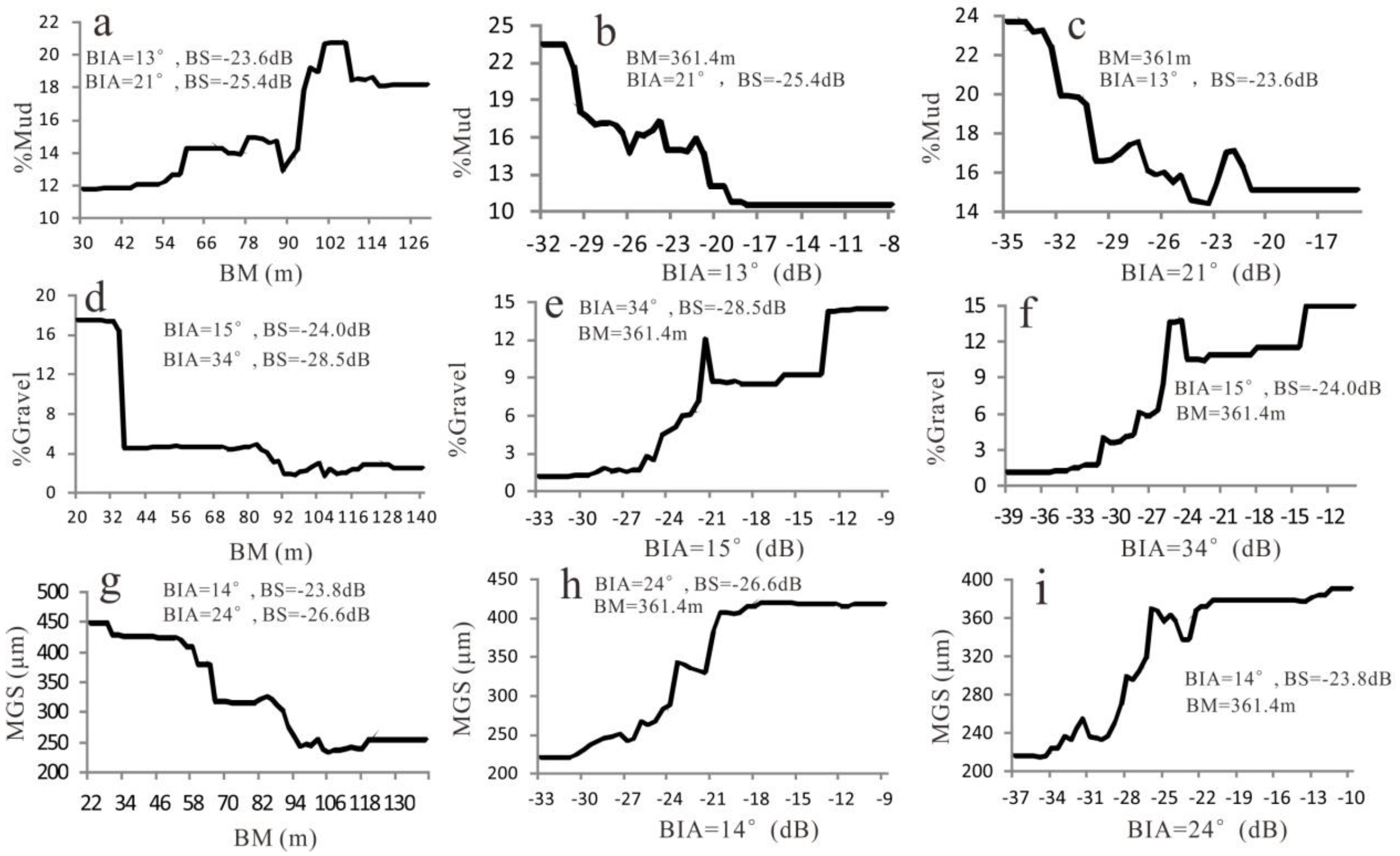
4.1.2. The Predicted Relationships between Multibeam Data and Sediment Properties

In this paper, we only present the predicted relationships between multibeam data and sediment grain size properties from the results of the second experiment, as it achieved superior prediction performance (Table 3 and Table 4). The selected explanatory variables for the predictions of individual sediment grain size properties, with the relative importance > 70%, are shown in

Table 5. The relative importance of characteristic variables for predicting the sediment properties explained by the model.

Sediment Grain Size Property	Relative Importance of Characteristic Variables
Mud	13° (100%), 21° (77.56%), depth (73.64%)
Gravel	15° (100%), 34° (97.95%), depth (88.09%)
MGS	14° (100%), 24° (94.90%), depth (86.53%)

. For %mud, the three most important explanatory variables were the BIA of 13° and 21° and BM, in order. For %gravel, the three most important explanatory variables were the BIA of 15° and 34° and BM, in order. For MGS, the three most important explanatory variables were the BIA of 14° and 24° and BM, in order.

The predicted relationships generated from these important explanatory variables are plotted in Figure 3. They show that all the predicted relationships are nonlinear. These relationships are described as follows:

• There was an obvious negative correlation between the %mud and the BIA of 13 and 21° (Figure 3b,c), but there was a positive correlation between the %mud and the BM until reaching a BM of ~100 m (Figure 3a);
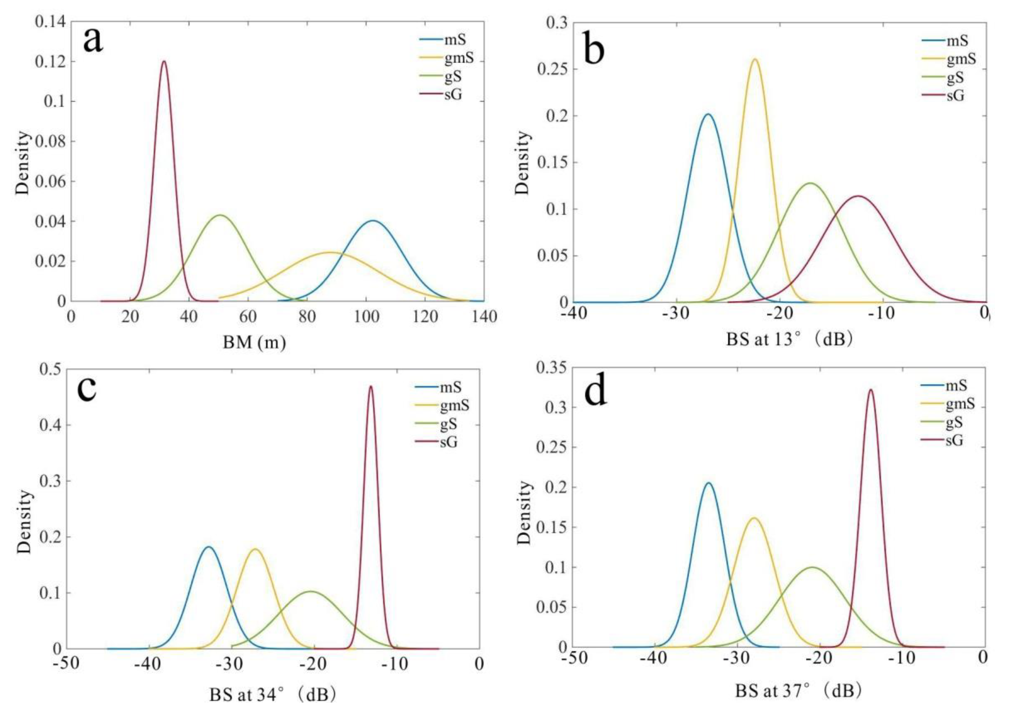
• The overall relationships between %gravel and the BIA of 15 and 34° were positive (Figure 3e,f). When the BS increases to ~−22 dB, the %gravel increases from 1% to 12%; increasing the BS further to −15 dB, however, decreases the %gravel to ~9%; further increasing the BS to −12 dB increases the %gravel again to ~15%. There is an abrupt relationship between the %gravel and BM. When the BM is shallower than ~32 m, the corresponding %gravel is more than 16%. However, when the BM is deeper than ~32 m, the %gravel sharply decreases to about 4% (Figure 3d);
• The overall predicted relationships between the MGS and the BIA of 14 and 24° are positive (Figure 3h,i), while a negative relationship was predicted between the MGS and BM (Figure 3g).

4.1.3. The Prediction Maps of the Sediment Grain Size Properties

In the first experiment, the predicted %gravel is between 16% and 42%, which is significantly larger than the measured value (0.05% to 46%) (Figure 4b). The predicted %mud ranges from 0.8% to 28%, which is significantly lower than the measured value (0.5% to 42%) (Figure 4d). The predicted %sand ranges from 47% to 79%, which is significantly smaller than the measured %sand (51% to 92%) (Figure 4f). The predicted value of mean particle size is between 355 and 760 μm, which is significantly larger than the measured mean particle size (124 to 827 μm) (Figure 4h).

In the second experiment, the predicted %gravel map shows that the %gravel is between 0.2% and 41%, while the measured values are between 0.05% and 46% (Figure 4a). The predicted %mud ranges from 0.6% to 39.5%, and the measured %mud ranges from 0.5% to 42% (Figure 4c). The predicted %sand ranges from 41% to 91%, and the measured %sand ranges from 51% to 92% (Figure 4e). The predicted mean particle size ranges from 146 to 760 μm; and the measured value ranges from 124 to 827 μm (Figure 4g). Therefore, it can be seen that the differences between the predicted results and the measured values are small.

The error statistics generated from comparing the measured values and the prediction maps are shown in Figure 5. In the first experiment, using only the multibeam BS as the explanatory variable, the modeling results of statistical error show that the MAE, RMSD, and N-RMSD for %gravel were relatively high, especially for N-RMSD which was 31.20% (Figure 5a’–d’). This indicates that the prediction of %gravel was relatively poor (Figure 5a’). Conversely, the MAE and RMSD for %mud were the lowest in comparison to %gravel and %sand. At the same, the lowest N-RNSD was also achieved for %mud. Although the MGS scored the largest MAE and RMSD, the N-RMSD was not the largest, because this is actually due to that the MGS was an order larger than the grain size properties. In addition, the prediction of MGS has achieved the second lowest N-RMSD (Figure 5d’).

In the second experiment, when using both multibeam BM and BS as explanatory variables, the results of statistical error show that the MAE, RMSD, and N-RMSD for %gravel were relatively low, especially for N-RMSD, which was only 11.25% (Figure 5a–d). However, the N-RMSD for MGS was the lowest (Figure 5d). It indicates that the prediction of MGS was relatively good. Although, the MAE and RMSD are higher than %gravel, %mud and %sand.

4.2. Prediction of Sediment Types

In the first experiment, when using only BS, we obtained the prediction results of each ground truth type. For the measured type of mS, it was all mismatched as acoustic class of gmS, with the number of 26. For the measured type of S, it was all mismatched as acoustic class of gmS, with the number of 4. For the measured type of gmS, the number of acoustic class that matched it correctly was thirteen and the remaining one were mismatched as acoustic class of gS. For the measured type of gS, the number of acoustic class that matched it correctly was two and the remaining two were mismatched as acoustic class of gmS and sG. For the measured type of msG, it was mismatched as acoustic class of gmS. For the measured type of sG, the number of acoustic class that matched it correctly was four, the other one was mismatched as acoustic class of gS. In short, only 19 of 54 sediment samples were predicted accurately which results in an overall prediction accuracy of 35.18% (Figure 6b).

In the second experiment, when using both BM and BS, we obtained the prediction results of each ground truth type. It shows that the measured type of mS, the number of acoustic class that matched it correctly was twenty two and the remaining four were mismatched as acoustic class of gmS. For the measured type of S, three were mismatched as acoustic class of mS, the other one was mismatched as acoustic class of gmS. For the measured type of gmS, the number of acoustic class that matched it correctly was thirteen and the remaining one were mismatched as acoustic class of gS. For the measured type of gS, acoustic class matched it correctly. For the measured type of msG, it was mismatched as acoustic class of gmS. For the measured type of sG, the number of acoustic class that matched it correctly was four, the other one was mismatched as acoustic class of gS. In short, the results show that 43 of 54 samples were predicted accurately, which resulted in a prediction accuracy of 79.63% (Figure 6a).

Conversely, we used the probability density functions (PDFs) to indicate the correlation between the exploratory variables and sediment Folk types. We found that the second experiment had good performance in overall accuracy (Figure 6a); therefore, we chose the exploratory variables including BM, BIA at 13, 34and 37°, which were chosen as the best combination of exploratory variables to predict the sediment types, to obtain the PDFs. The results are shown as following:

We choose the type of sediment that is accurately predicted, they are mS, gmS, gS and sG (Figure 6). For the type of mS, the peak of the density distribution of the BM is about 100m (Figure 7a), and the BM is also larger than the other three sediment types. As the BIA at 13°, the range of BS is between −33 and −20 dB (Figure 7b); As the BIA at 34°, the range of BS is between −40 and −25 dB (Figure 7c); As the BIA at 37°, the range of BS is between −40 and −27 dB (Figure 7d).

For the type of gmS, the peak of the density distribution of the BM is about 90 m (Figure 7a), and the BM is also larger than the other three sediment types. As the BIA at 13°, the range of BS is between −26 and −18 dB (Figure 7b); As the BIA at 34°, the range of BS is between −33 and −21 dB (Figure 7c); As the BIA at 37°, the range of BS is between −35 and −20 dB (Figure 7d).

For the type of gS, the peak of the density distribution of the BM is about 50 m (Figure 7a). As the BIA at 13°, the range of BS is between −26 and −8 dB (Figure 7b); As the BIA at 34°, the range of BS is between −30 and −10 dB (Figure 7c); As the BIA at 37°, the range of BS is between −40 and −27 dB (Figure 7d).

For the type of sG, the peak of the density distribution of the BM is about 30 m (Figure 7a), and the BM is also shallower than the other three sediment types. As the BIA at 13°, the range of BS is between −23 and −3 dB (Figure 7b); As the BIA at 34°, the range of BS is between −15 and −10 dB (Figure 7c); As the BIA at 37°, the range of BS is between −17 and −10 dB (Figure 7d).

5. Discussions

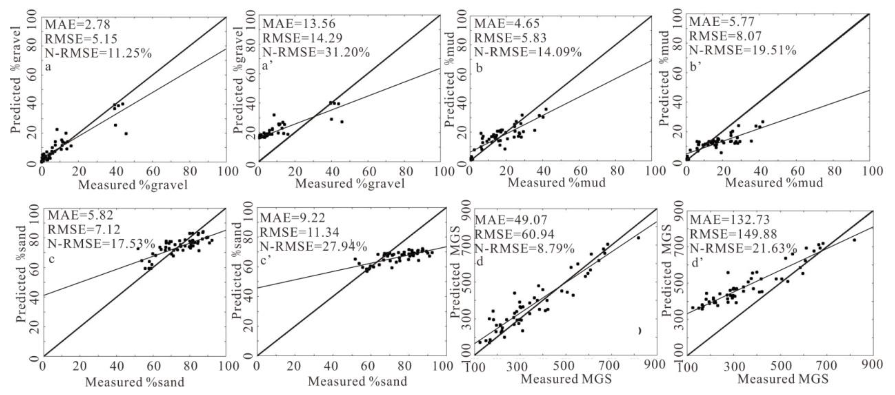
5.1. Evaluation of Model Prediction

Physical properties determined by sediment types include hardness (commonly known as acoustic impedance), surface roughness, and volume inhomogeneity. At the same time, previous studies have shown that the BS are closely related to these three physical properties [16,32]. Therefore, the sediment properties can be retrieved from the strength of the BS [2,10,23]. This is the foundation for using a multibeam for seabed sediment mapping. This study clearly demonstrated that using high-quality multibeam BM and BS data and the RFDT machine learning model, it is possible to effectively predict performance for sediment grain size properties and sediment types (Table 2 and Table 5). In the second experiment, the models explained 57%, 77%, and 85% of variances for %mud, %gravel, and MGS, respectively. The overall prediction accuracy for the seven sediment types was approximately 80%. The good prediction performance is mainly attributed to the strong relationship between the sediment distribution and multibeam data. The use of the RFDT machine learning model is also believed to have improved the prediction performance because of its ability to model nonlinear relationships. Thus, this study reaffirms the value of multibeam ecosystems as a modern acoustic remote sensing technology for mapping complex seabed environment [1,2,3,4,5,6,7,8,9,10].

This study also confirmed that, in general, using multibeam BM in addition to multibeam BS can improve the prediction performance of sediment mapping [15]. Furthermore, the prediction performance achieved a ~10% improvement for %gravel and %mud (Table 3 and Table 4) and a two-fold increase in the sediment type prediction (Figure 6). We calculated the kappa for the results of Experiment 1 and 2. According to the results of Figure 7, we found that they were 0.15 and 0.70, respectively; indicating that the consistency was slight in the first experiment and substantial in the second experiment. This is likely because BM is an important contributor to local dynamic oceanographic processes, which in turn influences sediment distribution. In addition, in this study, the final RFDT models selected a number of BS mosaics at different incidence angles (Table 2 and Table 3). This demonstrates the advantage of using the pseudo angular response curve, as in Huang et al. (2013, 2014) [15,24] for sediment mapping, because BS mosaics from different incidence angles are able to capture various aspects of sediment characteristics.

In addition to the ability to generate accurate sediment maps, the RFDT modeling was also able to help us gain a better understanding of the underlying correlation between multibeam data and sediment properties [15,16]. The results of this study confirmed that the mean grain size had a strong positive correlation with BS [10,12,13,15,16,21]. There was a negative relationship between% mud and BS (Figure 3a–c). In contrast, the %gravel had a positive correlation with BS (Figure 3d–f). This indicates that the coarser sediment returns a stronger BS than fine sediment. These findings are consistent with those of previous studies [13,17,19,20]. In addition to this, we found that if sediment property had a positive correlation with BS, it was negatively correlated with BM, and if sediment properties had a negative correlation with BS, it was positively correlated with BM (Figure 3).

5.2. Predicted Sediment Distributions and Application

Previous studies have used many methods to study the classification and mapping of sediment types; classification machine models include DT [33,34,35,36], RFDT [37,38,39,40,41], SVM [42,43], and ANN [44], while other methods include principal component analysis (PCA) [26], QTC Multiview [26,44], clustering [45], and MLC [35,43]. The original data include the BS image [26,39,40], angular response curve [10, 32&38], multibeam and BS-derived variables [15,41,63], and terrain attributes [63]. Classified objects include seabed hardness [41], sediment Folk classes [10,15], biota classes [38], simple types [39,64], and unsupervised classes [26,44]. In this study, the classification model was RFDT because of the advantages it provides in ranking explanatory variables by importance. The original data were the BS angular response from 5 to 45°, BM, and its derivatives in four sub-regions. The classified object was the Folk class (Table 1).

In the second experiment, we observed the overall prediction accuracy to be significantly improved. Therefore, BM and BS were set as explanatory variables to predict the acoustic classes in all four sub-regions. The best combination of explanatory variables selected by the iterative method to predict the sediment type was SA, BM, and BIA at 9 and 40°, with the highest overall accuracy of 64.16% (

Table 6. Selected feature variables for predicting the sediment types when samples were from all four sub-regions.

Iterations	Explanatory Variable	Classified Percentage
Initial experiment	Surface area	42.47
1st	depth	55.56
2nd	40°	63.80
3rd	9°	64.16
4th	10°	63.80

). The predictive maps of the acoustic classer in the four subsections are shown in Figure 8.

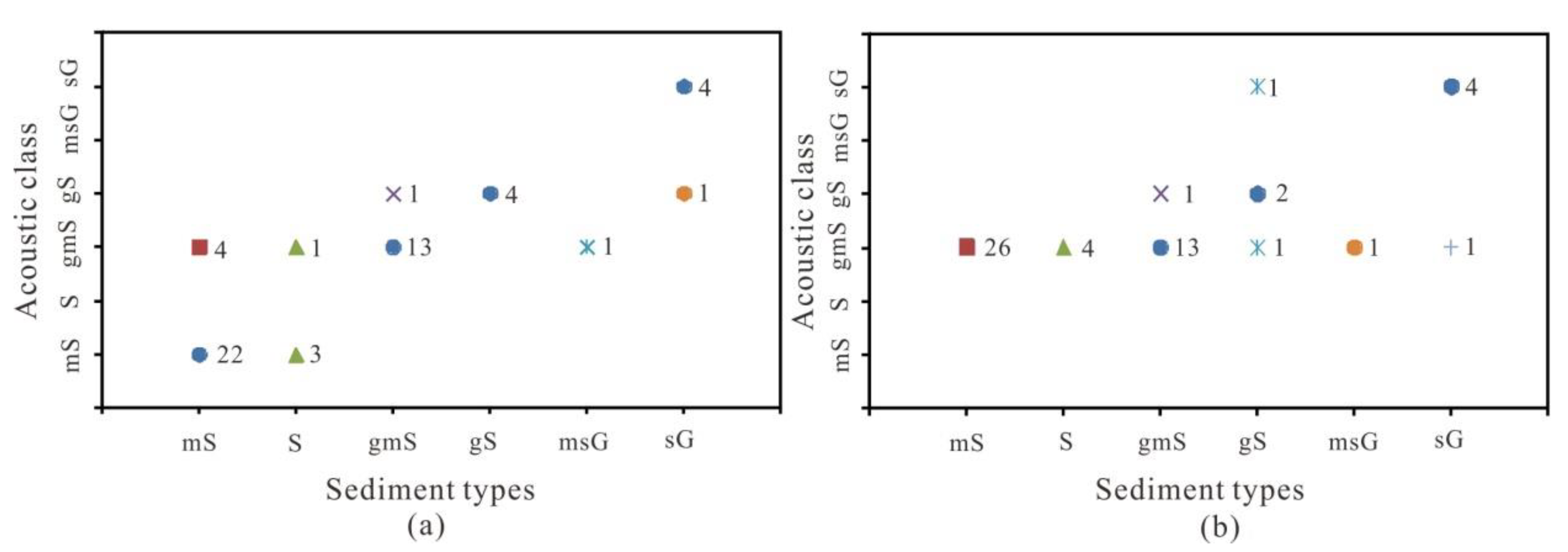
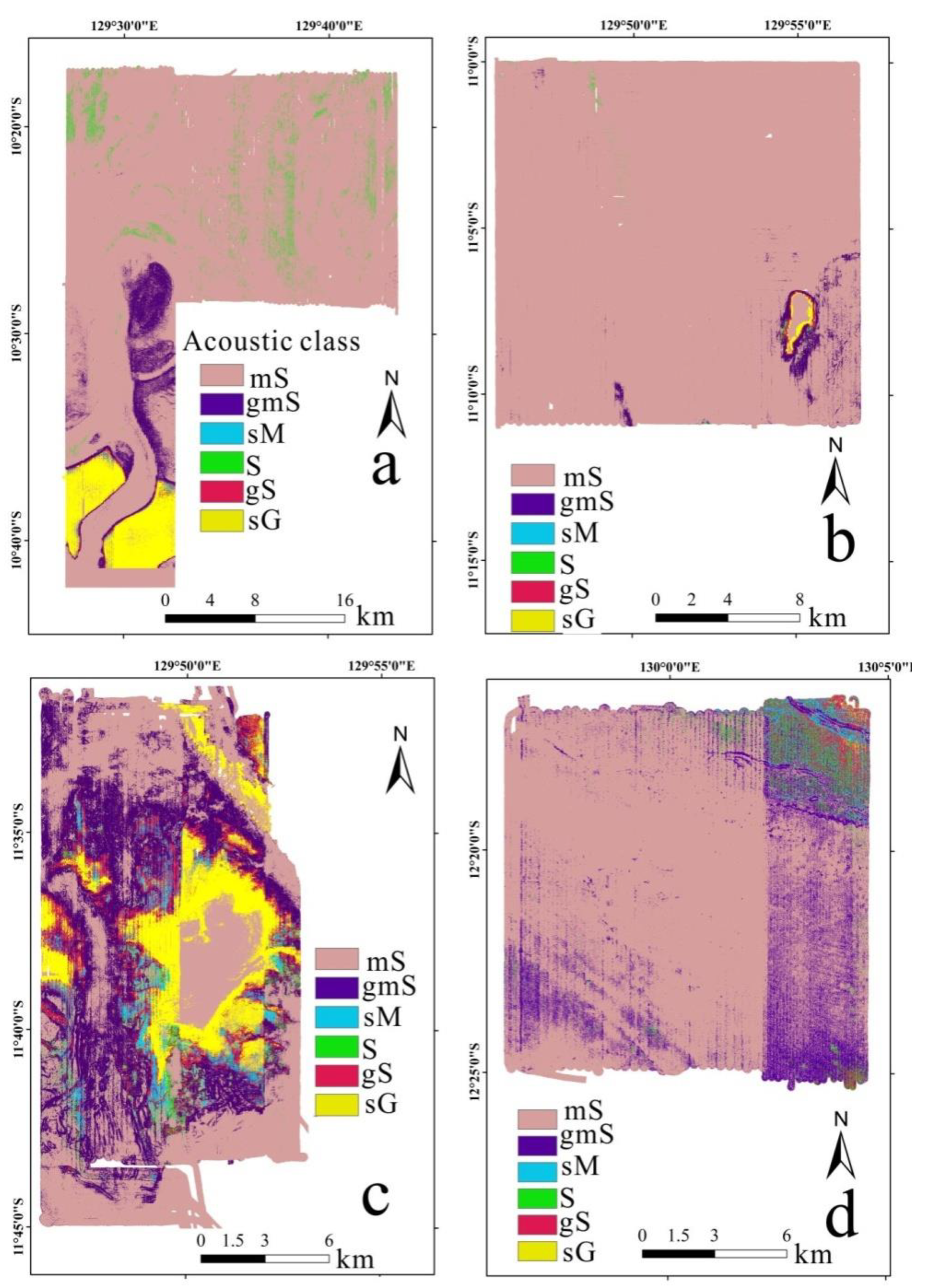
• For BP_A, there were six predicted classes. Among them, mS, S, gmS, and sG can be visually distinguished. The remaining two types (gS and sM) had smaller distribution areas. Compared with the measured sediment types, gmS disappeared in the acoustic types, but there was a type of sM in the acoustic class that was not in the measured types (Table 2 and Figure 8a);
• For BP_B, there were six predicted classes. Among them, gmS, mS, and sG could be clearly distinguished visually. The acoustic class of S was scattered sporadically in the area, and the acoustic class of sM was rarely distributed in this area. However, only four sediment types were measured (Table 2). Compared with the type of measurement, the type that disappeared in the acoustic type was the msG. However, there were three types of acoustic classes that were not included in the measured sediment. These were mS, sM and sG (Table 2 and Figure 8b);
• For BP_C, there were six predicted classes. The distribution of acoustic classes was complex. Through visual inspection, we found that the more distributed acoustic classes were mS, gmS, and sG. The remaining acoustic classes were sM, gS, and S. Compared with the measured sediment types, the type that disappeared in the acoustic type was msG (Table 2 and Figure 8c),
• For BP_D, there were six predicted classes. Most of the predicted classes were mS and gmS. The remaining classes were sM, S, gS and sG, and they were distributed in the northeast corner of the area. Compared with the measured sediment types, there were two types of sG and S in the acoustic class that were not measured (Table 2 and Figure 8d).

We found that the ground true class of msG was not recognized. In the predicted classes, it was wrongly divided into other classes because of the poor correlation between BM and %gravel (Figure 3d). When the BM was deeper than 32 m, the %gravel was less than 4%. In addition, the BM range of msG was between 70 and 170 m. This explains why msG was nearly misclassified as gmS in the Folk classification (Figure 6). However, the ground true class of sGs was correctly classified. This is because the BM range of sG was shallower than 35m, the predicted %gravel was high (Figure 3d). This indicates that the method in this study has poor applicability in deep-water areas with high %gravel.

6. Conclusions

High-resolution multibeam data were used to predict the seabed substrate in the Joseph Bonaparte Gulf, Northern Australia, using the RFDT. In summary, the major findings of this study are as follows:

(1)

Using multibeam BM in addition to multibeam BS improves the sediment prediction performance. The prediction performance achieved an improvement of ~10% for %gravel and %mud. The overall accuracy of the sediment type prediction will be improved from 35.18% to 79.63%, the Kappa will be improved from 0.15 to 0.70, and in comparison, only BS was set as the explanatory variable;

(2)

The relationships between sediment properties and multibeam data are nonlinear. The %mud has a negative correlation with BS between −35 and −17 dB, but it is positively correlated with BM between 30 and 100 m. The %gravel has a positive correlation with BS between −36 and −12 dB. However, the relationship between %gravel and depth is poor, which indicates that this method is not suitable for deep water areas with high %gravel because of the unclear underlying relationship between %gravel and BM. The MGS has a positive correlation with BS between −37 and −19 dB, while it is negatively correlated with BM between 22 and 118 m.

In summary, high-resolution multi-beam data can be used to predict a large area of the seabed substrate by applying the RFDT. At the same time, it can also indicate a nonlinear relationship between sediment properties and multibeam data.

References

1. Brown, C.J.; Smith, S.J.; Lawton, P.; Anderson, J.T. Benthic habitat mapping: A review of progress towards improved understanding of the spatial ecology of the seafloor using acoustic techniques. Estuar. Coast. Shelf Sci. 2011, 92, 502–520. [Google Scholar] [CrossRef]
2. Cui, X.; Liu, H.; Fan, M.; Ai, B.; Ma, D.; Yang, F. Seafloor habitat mapping using multibeam bathymetric and backscatter intensity multi-features SVM classification framework. Appl. Acoust. 2021, 174, 107728. [Google Scholar] [CrossRef]
3. Erdey-Heydorn, M.D. An ArcGIS seabed characterization toolbox developed for investigating benthic habitats. Mar. Geod. 2008, 31, 318–358. [Google Scholar] [CrossRef]
4. Lanier, A.; Romsos, C.; Goldfinger, C. Seafloor habitat mapping on the oregon continental margin: A spatially nested GIS approach to mapping scale, mapping methods, and accuracy quantification. Mar. Geod. 2007, 30, 51–76. [Google Scholar] [CrossRef]
5. Le Gonidec, Y.; Lamarche, G.; Wright, I.C. Inhomogeneous substrate analysis using EM300 backscatter imagery. Mar. Geophys. Res. 2003, 24, 311–327. [Google Scholar] [CrossRef]
6. Courtney, R.C.; Shaw, J. Multibeam bathymetry and back-scatter imaging of the Canadian continental shelf. Geosci. Can. 2000, 27, 31–42. [Google Scholar]
7. Goff, J.A.; Orange, D.L.; Mayer, L.A.; Clarke, J.E.H. Detailed investigation of continental shelf morphology using a high-resolution swath sonar survey: The Eel margin, northern California. Mar. Geol. 1999, 154, 255–269. [Google Scholar] [CrossRef]
8. Ji, X.; Yang, B.; Tang, Q. Seabed sediment classification using multibeam backscatter data based on the selecting optimal random forest model. Appl. Acoust. 2020, 167, 107387. [Google Scholar] [CrossRef]
9. Mitchell, N.C.; Clarke, J.E.H. Classification of seafloor geology using multibeam sonar data from the Scotian Shelf. Mar. Geol. 1994, 121, 143–160. [Google Scholar] [CrossRef]
10. Snellen, M.; Gaida, T.C.; Koop, L.; Alevizos, E.; Simons, D.G. Performance of multibeam echosounder backscatter-based classification for monitoring sediment distributions using multitemporal large-scale ocean data sets. IEEE J. Ocean. Eng. 2019, 44, 142–155. [Google Scholar] [CrossRef] [Green Version]
11. Huang, Z.; Brooke, B.P.; Harris, P.T. A new approach to mapping marine benthic habitats using physical environmental data. Cont. Shelf Res. 2011, 31, S4–S16. [Google Scholar] [CrossRef]
12. Collier, J.S.; Brown, C.J. Correlation of sidescan backscatter with grain size distribution of surficial seabed sediments. Mar. Geol. 2005, 214, 431–449. [Google Scholar] [CrossRef]
13. Ferrini, V.L.; Flood, R.D. A comparison of Rippled Scour Depressions identified with multibeam sonar: Evidence of sediment transport in inner shelf environments. Cont. Shelf Res. 2005, 25, 1979–1995. [Google Scholar] [CrossRef]
14. Haris, K.; Chakraborty, B.; Ingole, B.; Menezes, A.; Srivastava, R. Seabed habitat mapping employing single and multibeam backscatter data: A case study from the western continental shelf of India. Cont. Shelf Res. 2012, 48, 40–49. [Google Scholar] [CrossRef]
15. Huang, Z.; Siwabessy, J.; Nichol, S.L.; Brooke, B.P. Predictive mapping of seabed substrate using high-resolution multibeam sonar data: A case study from a shelf with complex geomorphology. Mar. Geol. 2014, 357, 37–52. [Google Scholar]
16. Huang, Z.; Siwabessy, J.; Cheng, H.; Nichol, S.; Heqin, C. Using multibeam backscatter data to investigate sediment-acoustic relationships. J. Geophys. Res. Oceans 2018, 123, 4649–4665. [Google Scholar] [CrossRef]
17. Urick, R.J. Principles of Underwater Sound; McGraw-Hill: New York, NY, USA, 1983. [Google Scholar]
18. Fonseca, L.; Brown, C.; Calder, B.; Mayer, L.; Rzhanov, Y. Angular range analysis of acoustic themes from Stanton Banks Ireland: A link between visual interpretation and multibeam echo sounder angular signatures. Appl. Acoust. 2009, 70, 1298–1304. [Google Scholar] [CrossRef]
19. De Falco, G.; Tonielli, R.; Di Martino, G.; Innangi, S.; Simeone, S.; Parnum, I. Relationships between multibeam backscatter, sediment grain size and Posidonia oceanica seagrass distribution. Cont. Shelf Res. 2010, 30, 1941–1950. [Google Scholar] [CrossRef]
20. Davis, K.S.; Slowey, N.C.; Stender, I.H.; Fiedler, H.; Bryant, W.R.; Fechner, G. Acoustic backscatter and sediment textural properties of inner shelf sands, northeastern Gulf of Mexico. Geo Mar. Lett. 1996, 16, 273–278. [Google Scholar] [CrossRef]
21. Goff, J.A.; Olson, H.C.; Duncan, C.S. Correlation of side-scan backscatter intensity with grain-size distribution of shelf sediments, New Jersey margin. Geo Mar. Lett. 2000, 20, 43–49. [Google Scholar] [CrossRef]
22. Ryan, W.B.F.; Flood, R.D. Side-looking sonar backscatter response at dual frequencies. Mar. Geophys. Res. 1996, 18, 689–705. [Google Scholar] [CrossRef]
23. Hamilton, L.J.; Parnum, I. Acoustic seabed segmentation from direct statistical clustering of entire multibeam sonar backscatter curves. Cont. Shelf Res. 2011, 31, 138–148. [Google Scholar] [CrossRef]
24. Huang, Z.; Siwabessy, J.; Nichol, S.; Anderson, T.; Brooke, B. Predictive mapping of seabed cover types using angular response curves of multibeam backscatter data: Testing different feature analysis approaches. Cont. Shelf Res. 2013, 61–62, 12–22. [Google Scholar] [CrossRef]
25. Mccullagh, D.; Benetti, S.; Plets, R.; Sacchetti, F.; O’Keeffe, E.; Lyons, K. Geomorphology and substrate of Galway Bay, Western Ireland. J. Maps 2020, 16, 166–178. [Google Scholar] [CrossRef]
26. McGonigle, C.; Brown, C.; Quinn, R.; Grabowski, J. Evaluation of image-based multibeam sonar backscatter classification for benthic habitat discrimination and mapping at Stanton Banks, UK. Estuar. Coast. Shelf Sci. 2009, 81, 423–437. [Google Scholar] [CrossRef]
27. Preston, J. Automated acoustic seabed classification of multibeam images of Stanton Banks. Appl. Acoust. 2009, 70, 1277–1287. [Google Scholar] [CrossRef]
28. Clarke, J.H. Toward remote seafloor classification using the angular response of acoustic backscattering: A case study from multiple overlapping GLORIA data. IEEE J. Ocean. Eng. 1994, 19, 112–127. [Google Scholar] [CrossRef]
29. Fonseca, L.; Mayer, L.A. Remote estimation of surficial seafloor properties through the application Angular Range Analysis to multibeam sonar data. Mar. Geophys. Res. 2007, 28, 119–126. [Google Scholar] [CrossRef]
30. Dartnell, P.; Gardner, J.V. Predicting seafloor facies from multibeam bathymetric and backscatter data. Photogramm. Eng. Remote Sens. 2004, 70, 1081–1091. [Google Scholar] [CrossRef] [Green Version]
31. Huang, Z.; Nichol, S.L.; Siwabessy, J.P.; Daniell, J.; Brooke, B.P. Predictive modelling of seabed sediment parameters using multibeam acoustic data: A case study on the Carnarvon Shelf, Western Australia. Int. J. Geogr. Inf. Sci. 2012, 26, 283–307. [Google Scholar] [CrossRef]
32. Alevizos, E.; Greinert, J. The hyper-angular cube concept for improving the spatial and acoustic resolution of mbes backscatter angular response analysis. Geosciences 2018, 8, 446. [Google Scholar] [CrossRef] [Green Version]
33. Hasan, R.C.; Ierodiaconou, D.; Laurenson, L. Combining angular response classification and backscatter imagery segmentation for benthic biological habitat mapping. Estuar. Coast. Shelf Sci. 2012, 97, 1–9. [Google Scholar] [CrossRef] [Green Version]
34. Friedman, J.H. Stochastic gradient boosing. Comput. Stat. Data Anal. 2002, 38, 367–378. [Google Scholar] [CrossRef]
35. Ierodiaconou, D.; Monk, J.; Rattray, A.; Laurenson, L.; Versace, V.L. Comparison of automated classification techniques for predicting benthic biological communities using hydro-acoustics and video observations. Cont. Shelf Res. 2011, 31, S28–S38. [Google Scholar] [CrossRef]
36. Rattray, A.; Ierodiaconou, D.; Laurenson, L.; Burq, S.; Reston, M. Hydro-acoustic remote sensing of benthic biological communities on the shallow South East Australian continental shelf. Estuar. Coast. Shelf Sci. 2009, 84, 237–245. [Google Scholar] [CrossRef]
37. Breiman, L. Random forests. Mach. Learn. 2001, 45, 5–32. [Google Scholar] [CrossRef] [Green Version]
38. Hasan, R.C.; Ierodiaconou, D.; Laurenson, L.; Schimel, A. Integrating multibeam backscatter angular response; mosaic and bathymetry data for benthic habitat mapping. PLoS ONE 2014, 9, e97339. [Google Scholar]
39. Diesing, M.; Green, S.L.; Stephens, D.; Lark, R.; Stewart, H.A.; Dove, D. Mapping seabed sediments: Comparison of manual, geostatistical, object-based image analysis and machine learning approaches. Cont. Shelf Res. 2014, 84, 107–119. [Google Scholar] [CrossRef] [Green Version]
40. Lucieer, V.; Hill, N.A.; Barrett, N.S.; Nichol, S. Do marine substrates ‘look’ and ‘sound’ the same? Supervised classification of multibeam acoustic data using autonomous underwater vehicle images. Estuar. Coast. Shelf Sci. 2013, 117, 94–106. [Google Scholar] [CrossRef]
41. Li, J.; Tran, M.; Siwabessy, J. Selecting optimal random forest predictive models: A case study on predicting the spatial distribution of seabed hardness. PLoS ONE 2016, 11, e0149089. [Google Scholar] [CrossRef]
42. Cortes, C.; Vapnik, V. Support-vector networks. Mach. Learn. 1995, 20, 273–297. [Google Scholar] [CrossRef]
43. Hasan, R.C.; Ierodiaconou, D.; Monk, J. Evaluation of four supervised learning methods for benthic habitat mapping using backscatter from multi- beam sonar. Remote Sens. 2012, 4, 3427–3443. [Google Scholar] [CrossRef] [Green Version]
44. Marsh, I.; Brown, C. Neural network classification of multibeam backscatter and bathymetric data from Stanton Bank (Area IV). Appl. Acoust. 2009, 70, 1269–1276. [Google Scholar] [CrossRef]
45. Brown, C.J.; Collier, J.S. Mapping benthic habitat in regions of gradational substrata: An automated approach utilizing geophysical, geological, and biological relationships. Estuar. Coast. Shelf Sci. 2008, 78, 203–214. [Google Scholar] [CrossRef]
46. Francke, T.; López-Tarazón, J.; Schröder, B. Estimation of suspended sediment concentration and yield using linear models, random forests and quantile regression forests. Hydrol. Process. 2008, 22, 4892–4904. [Google Scholar] [CrossRef]
47. Anderson, T.J.; Nichol, S.; Radke, L.; Heap, A.D.; Battershill, C.; Hughes, M.; Siwabessy, P.J.; Barrie, V.; De Glasby, B.A.; Tran, M.; et al. Seabed Environment of the Eastern Joseph Bonaparte Gulf, Northern Australia; SOL 4934—Post-Survey Report; Geoscience Australia: Canberra, Australia, 2010; p. 78. [Google Scholar]
48. Przeslawski, R.; Daniell, J.; Anderson, T.; Barrie, J.V.; Heap, A.; Hughes, M.; Li, J.; Potter, A.; Radke, L.; Siwabessy, J.; et al. Seabed Habitats and Hazards of the Joseph Bonaparte Gulf and Timor Sea, Northern Australia; Geoscience Australia: Canberra, Australia, 2011; p. 69, Record 2011/40. [Google Scholar]
49. Anderson, T.J.; Nichol, S.; Radke, L.; Heap, A.D.; Battershill, C.; Hughes, M.; Siwabessy, P.J.; Barrie, V.; De Glasby, B.A.; Tran, M.; et al. Seabed Environments of the Eastern Joseph Bonaparte Gulf, Northern Australia; GA0325/Sol5117—Post-Survey Report; Geoscience Australia: Canberra, Australia, 2011. [Google Scholar]
50. Lees, B.G. Recent terrigenous sedimentation in Joseph Bonaparte Gulf, Northwestern Australia. Mar. Geol. 1992, 103, 199–213. [Google Scholar] [CrossRef]
51. Lewis, D.W.; Mcconchie, D. Analytical Sedimentology; Springer: New York, NY, USA, 1994. [Google Scholar]
52. Folk, R.L. Petrology of Sedimentary Rocks: Austin; Hemphill Publishing: Austin, TX, USA, 1968; Volume 21, pp. 714–727. [Google Scholar]
53. Lamarche, G.; Lurton, X. Recommendations for improved and coherent acquisition and processing of backscatter data from seafloor-mapping sonars. Mar. Geophys. Res. 2017, 39, 5–22. [Google Scholar] [CrossRef] [Green Version]
54. Gavrilov, A.N.; Siwabessy, P.J.W.; Parnum, I.M. Multibeam Echo Sounder Backscatter Analysis: Theory Review, Methods and Application to Sydney Harbour Swath Data; Centre for Marine Science and Technology: Perth, Australian, 2005. [Google Scholar]
55. Gavrilov, A.N.; Duncan, A.J.; McCauley, R.D.; Parnum, I.M.; Penrose, J.D.; Siwabessy, P.J.W.; Woods, A.J.; Tseng, Y.-T. Characterization of the seafloor in Australia’s coastal zone using acoustic techniques. In Proceedings of the 1st International Conference in Underwater Acoustic Measurements: Technologies & Results, Crete, Greece, 28 June–1 July 2005. [Google Scholar]
56. De Moustier, C.; Alexandrou, D. Angular dependence of 12-kHz seafloor acoustic backscatter. J. Acoust. Soc. Am. 1991, 90, 522–531. [Google Scholar] [CrossRef]
57. Jackson, D.; Winebrenner, D.P.; Ishimaru, A. Application of the composite roughness model to high-frequency bottom backscattering. J. Acoust. Soc. Am. 1986, 79, 1410–1422. [Google Scholar] [CrossRef]
58. Lurton, X.; Lamarche, G.; Brown, C.; Rice, G.; Schimel, A.; Weber, T. Backscatter Measurements by Seafloor-Mapping Sonars—Guidelines and Recommendations; Technical Report; GEOHAB: Oostende, Belgium, 2015; pp. 1–200. [Google Scholar]
59. Parnum, I.M.; Gavrilov, A.N. High-frequency multibeam echo-sounder measurements of seafloor backscatter in shallow water: Part 2—Mosaic production, analysis and classification. Underw. Technol. Int. J. Soc. Underw. 2011, 30, 13–26. [Google Scholar] [CrossRef]
60. Weiss, A.D. Topographic position and landforms analysis. In Proceedings of the ESRI International User Conference, San Diego, CA, USA, 9–13 July 2001. [Google Scholar]
61. Jenness, J.S. Calculating landscape surface area from digital elevation models. Wildl. Soc. Bull. 2004, 32, 829–839. [Google Scholar] [CrossRef]
62. Huang, Z.; McArthur, M.; Radke, L.; Anderson, T.; Nichol, S.; Siwabessy, J.; Brooke, B. Developing physical surrogates for benthic biodiversity using co-located samples and regression tree models: A conceptual synthesis for a sandy temperate embayment. Int. J. Geogr. Inf. Sci. 2012, 26, 2141–2160. [Google Scholar] [CrossRef]
63. Lecours, V.; Brown, C.; Devillers, R.; Lucieer, V.; Edinger, E.N. Comparing selections of environmental variables for ecological studies: A focus on terrain attributes. PLoS ONE 2016, 11, e0167128. [Google Scholar] [CrossRef] [Green Version]
64. Lucieer, V.L. Object-oriented classification of sidescan sonar data for mapping benthic marine habitats. Int. J. Remote Sens. 2007, 29, 905–921. [Google Scholar] [CrossRef]
Figure 1. Workflow diagram of the research methods from raw data processing to model prediction.
Jmse 09 00947 g001
Figure 2. The study area and the sediment sample locations: (a). The relative location of study area in northern Australian and (b). The location of the four subregions on the continental shelf. (A). The mapping area BP_A; (B). The mapping area BP_B; (C). The mapping area BP_C; (D). The mapping area BP_D.
Jmse 09 00947 g002
Figure 3. The predictive relationship curves between the characteristic variables and sediment properties. (a), %mud and BM; (b), %mud and BIA = 13°; (c), %mud and BIA = 21°; (d), %gravel and BM; (e), %gravel and BIA = 15°; (f), %gravel and BIA = 34°; (g), MGS and BM; (h), MGS and BIA = 14°; (i), MGS and BIA = 24°. BM indicates bathymetry, BIA indicates incidence angle of backscatter, and BS indicates backscatter intensity.
Jmse 09 00947 g003
Figure 4. Predictive mapping of acoustic sediment properties in the BP_A overlapped with the measured sediment properties. When BM and BS were set as explanatory variable: (a), the predictive mapping of acoustic %gravel; (c), the predictive mapping of acoustic %mud; (e), the predictive mapping of acoustic %sand; (g), the predictive mapping of acoustic MGS. When only BS was set as explanatory variable: (b), the predictive mapping of acoustic %gravel; (d), the predictive mapping of acoustic %mud; (f), the predictive mapping of acoustic %sand; (h), the predictive mapping of acoustic MGS.
Jmse 09 00947 g004
Figure 5. The correlation between measured and acoustic values of sediment properties and the statistical error evaluation. (ad) indicate the result of that BM and BS were set as the explanatory variable. (a’d’) indicate the result of that BS was set as the explanatory variable. (a,a’), measured %gravel and acoustic %gravel; (b,b’), measured %mud and acoustic %mud; (c,c’), measured %sand and acoustic %sand; (d,d’), measured MGS and acoustic MGS. MAE indicates the mean absolute error. RMSE indicates the root mean square error. N-RMSE indicates the normalized root mean square error.
Jmse 09 00947 g005
Figure 6. The correlation between acoustic class and measured sediment types at BP_A. (a) BM and BS were set as the explanatory variables, and (b) BS was set as the explanatory variables. The blue dots indicate correct matches between acoustic class and measured sediment types, other colored symbols indicate wrong matches, and the Arabic number indicates the number of matches.
Jmse 09 00947 g006
Figure 7. The probability density functions (PDFs) of measured BS and BM for sediment types. (a), The PDFs of sediment types and BM; (b), The PDFs of sediment types and BS at 13°; (c), The PDFs of sediment types and BS at 34°; (d), The PDFs of sediment types and BS at 37°.
Jmse 09 00947 g007
Figure 8. Predicted mapping of acoustic class and the distribution of seabed samples: (a), the map of BP_A; (b), the map of BP_B; (c), the map of BP_C; (d), the map of BP_D.
Jmse 09 00947 g008