
Fractional-Order Elastoplastic Modeling of Sands Considering Cyclic Mobility


Abstract
1. Introduction
2. New Fractional Cyclic Model
2.1. Elastic Strain
2.2. Subloading Yield Surface
2.3. Fractional-Order Plastic Flow Rule
2.4. Hardening Rules
2.5. Incremental Stress–Strain Relationship
3. Validation
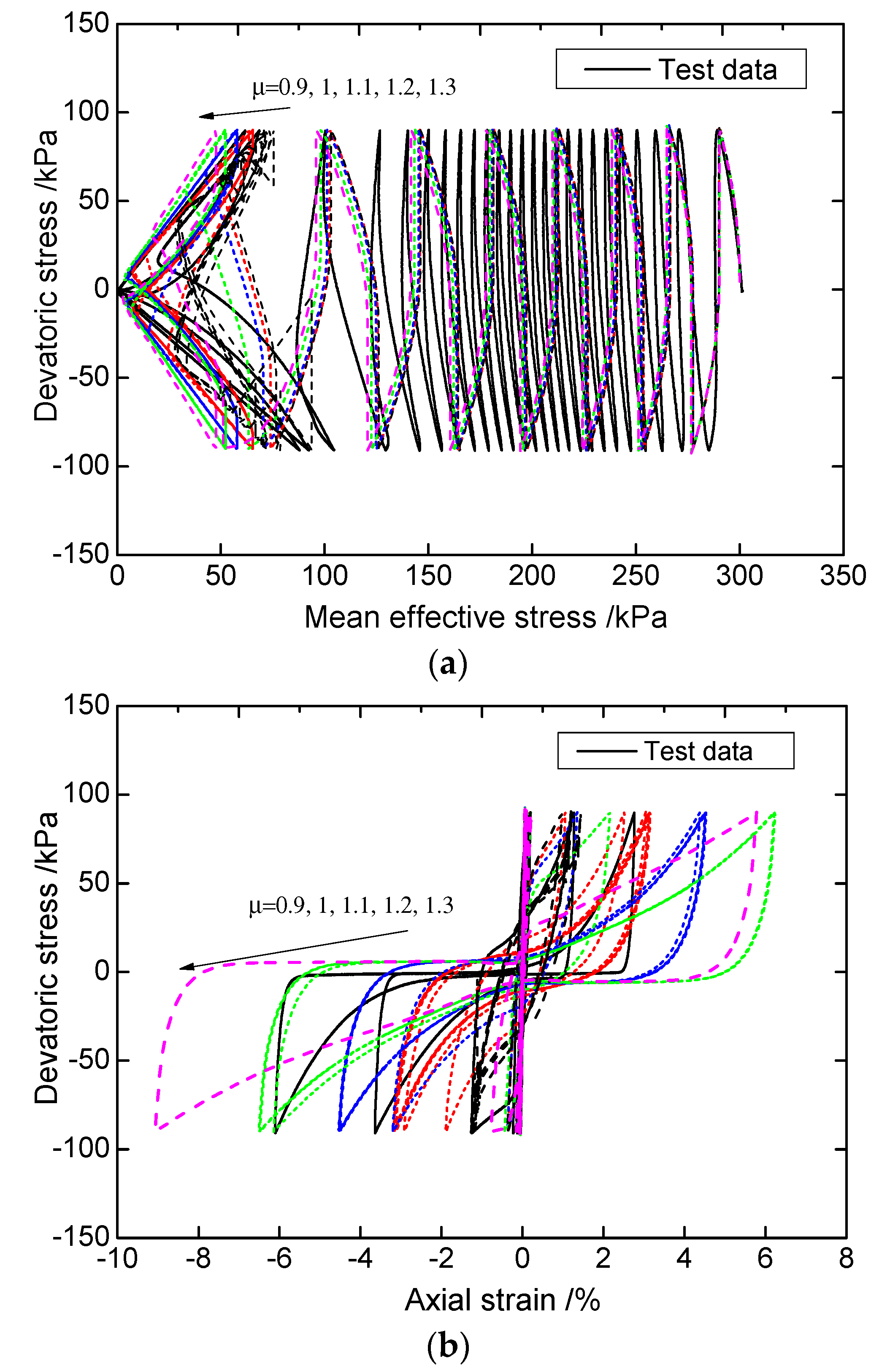
3.1. Stress-Controlled Cyclic Test
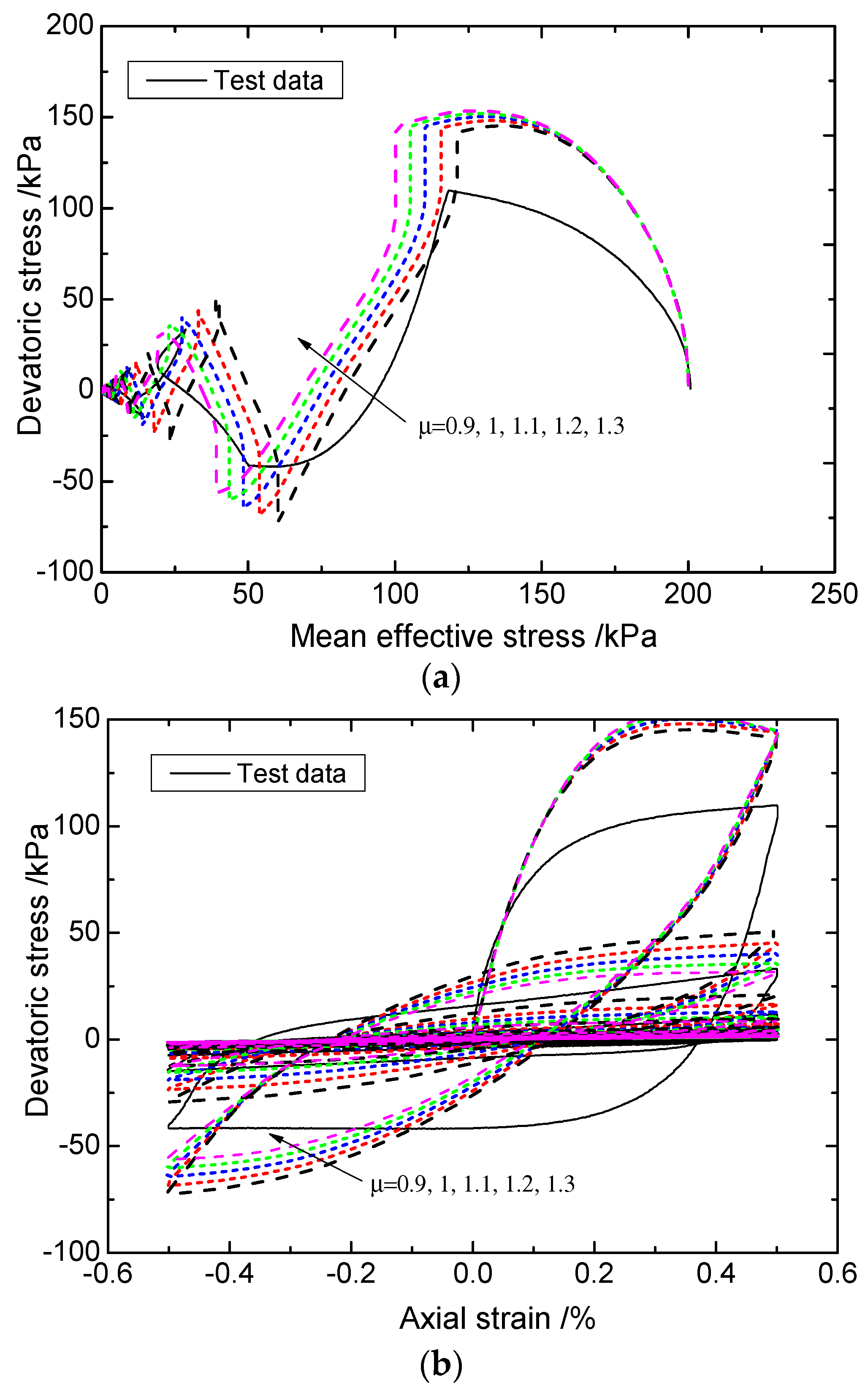
3.2. Strain-Controlled Cyclic Test
4. Application
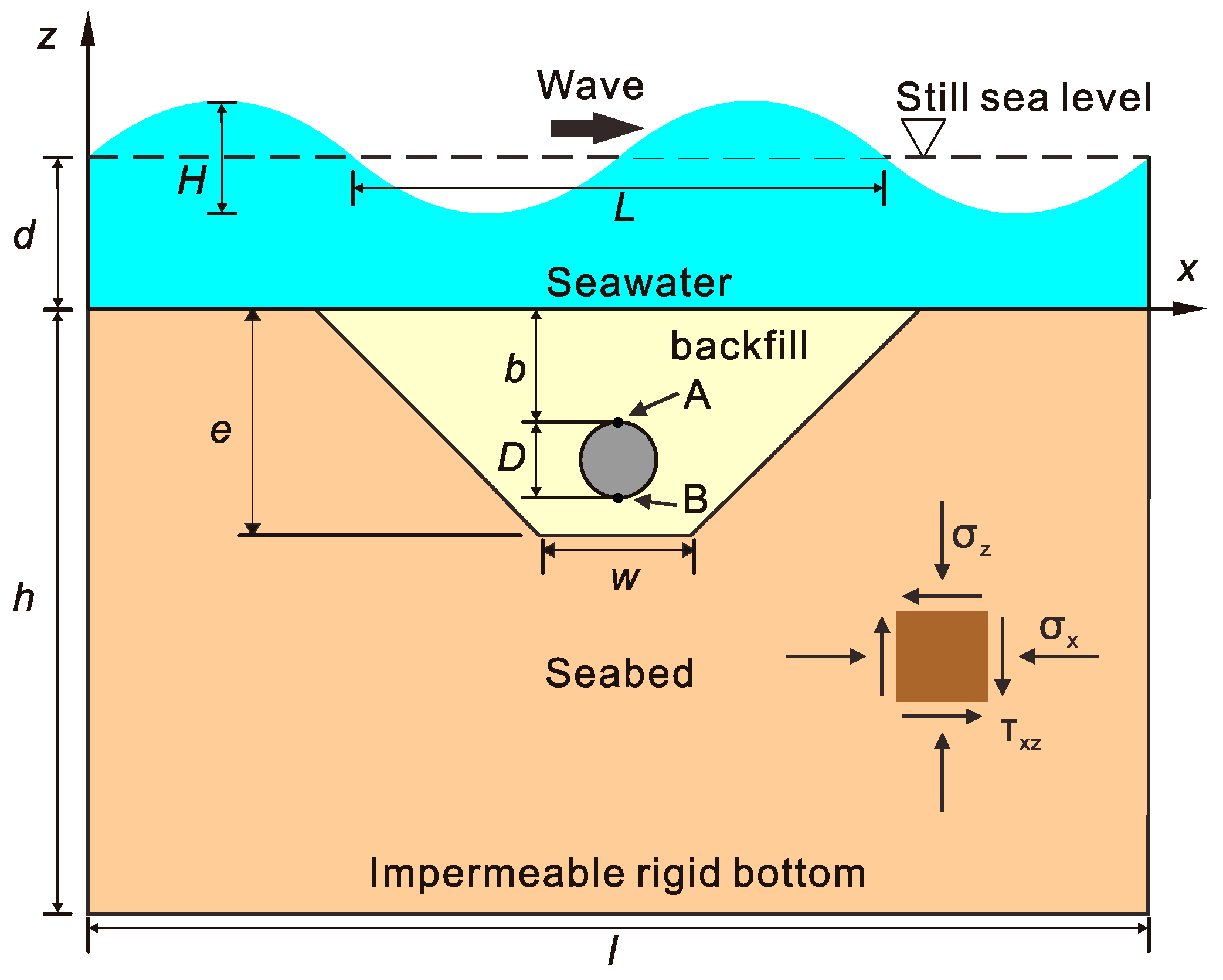
4.1. Model Setup
4.2. Homogeneous Seabed
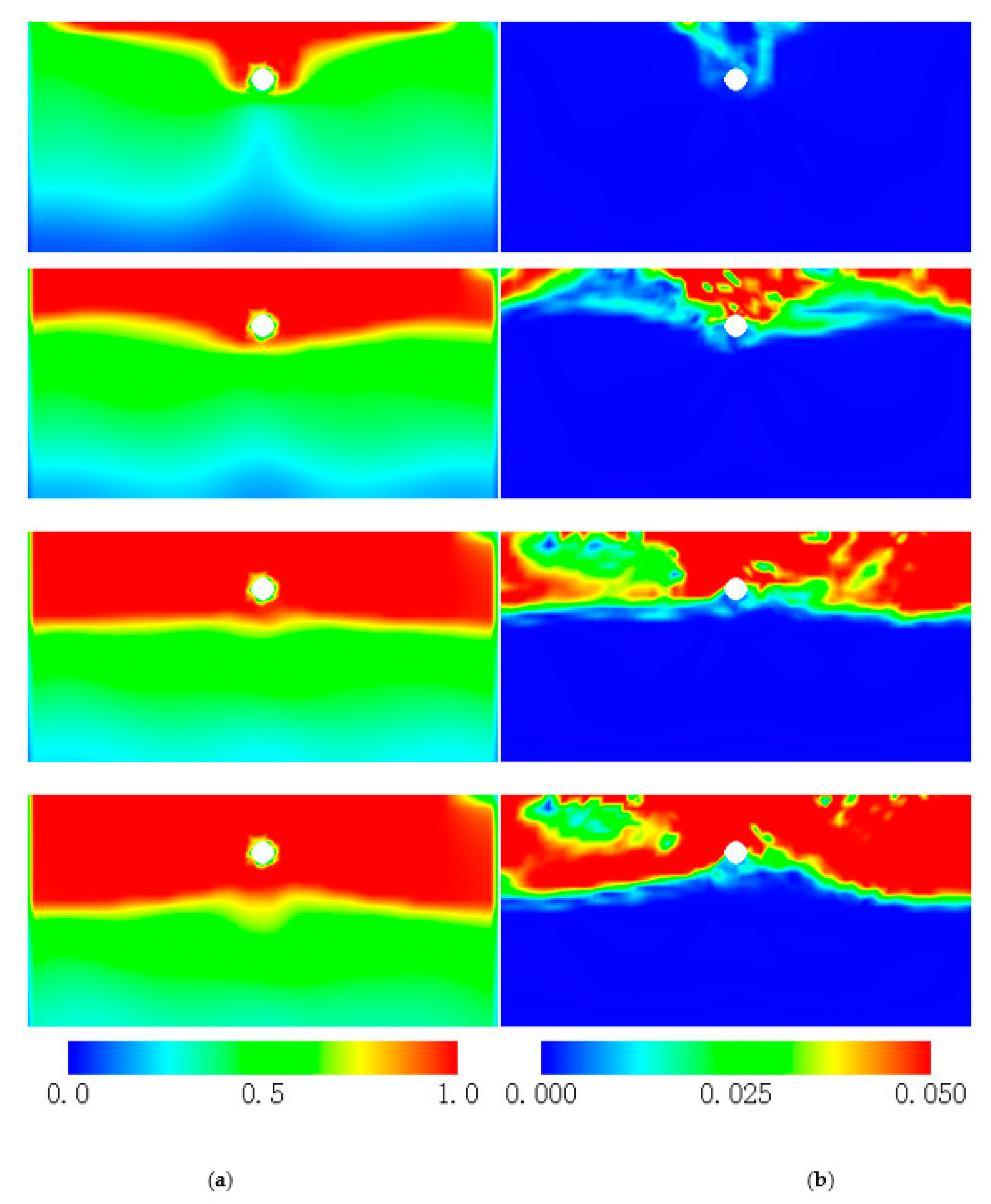
4.2.1. Wave-Induced Liquefaction
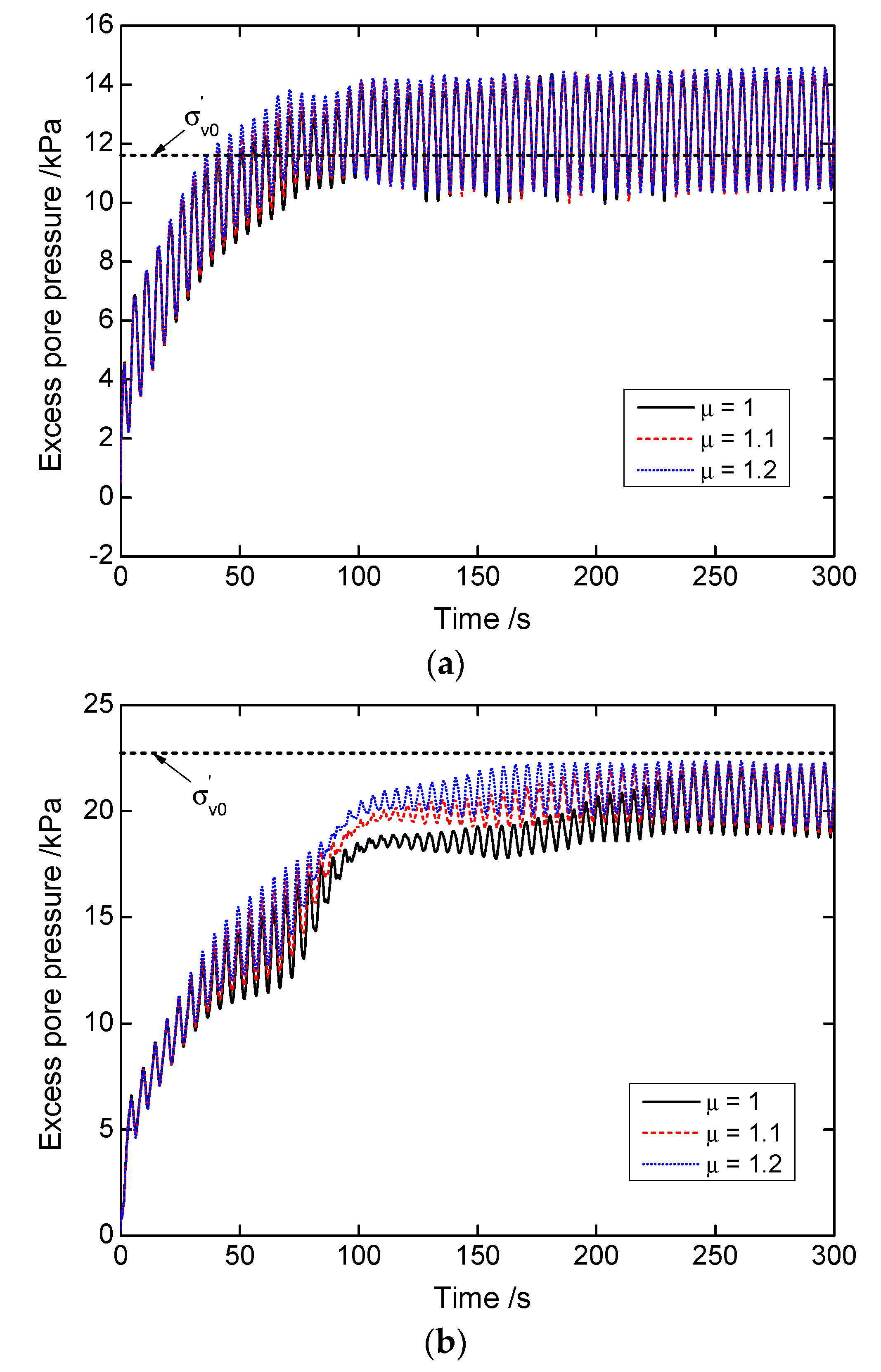
4.2.2. Excess Pore Pressure
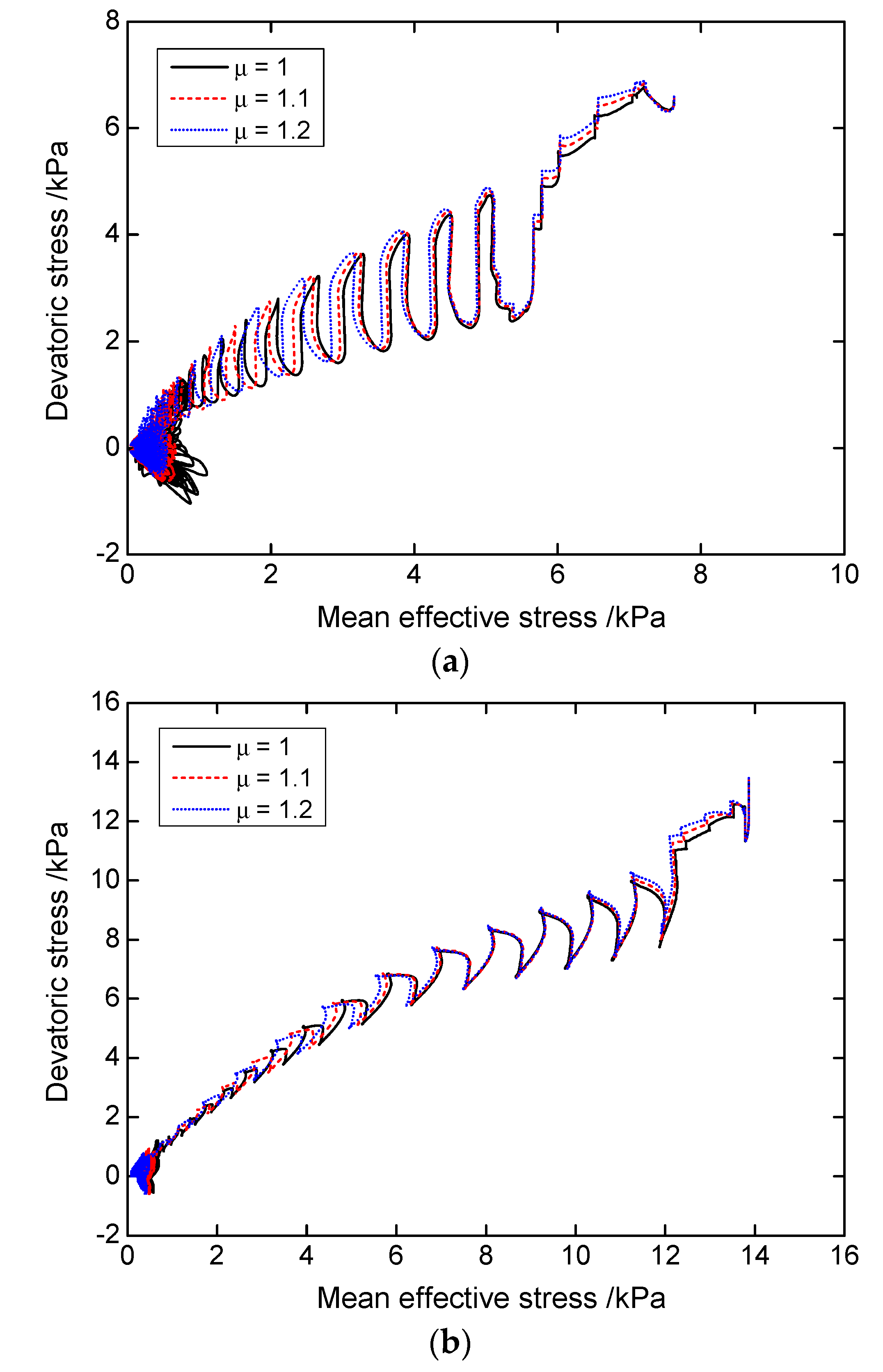
4.2.3. Effective Stress Path
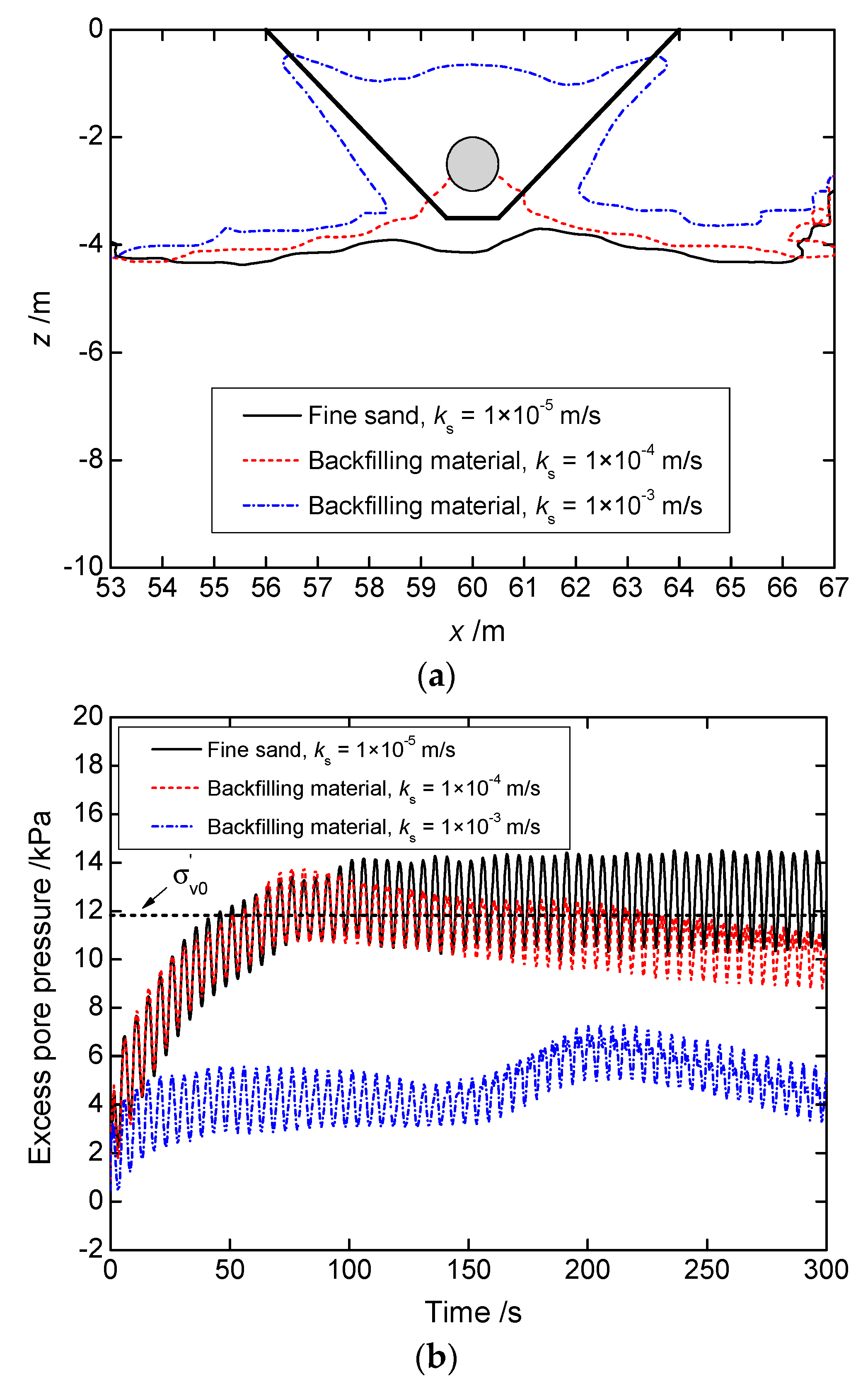
4.3. Seabed with a Trench Layer
5. Conclusions
- The non-associated flow rule was successfully incorporated into the proposed model based on the fractional-order plasticity theory, and the fractional order that determines the plastic flow direction can be obtained by the dilatancy ratio. Combined with the multiple hardening rules, the state dependency, cyclic mobility, and non-associated behavior of sands are reasonably mimicked by the proposed model.
- With the increase in the fractional order, the dilatancy ratio and the critical state ratio would both increase. In undrained cyclic conditions, a larger fractional order would result in a quicker accumulation of excess pore pressure in the soil sample modeled. Accordingly, the stress point would approach the liquefaction state more quickly.
- The proposed model shows good robustness during large-scale numerical simulation of dynamic geotechnical problems. Based on the results of numerical simulation, it was found that non-associativity of sand has an important effect on the accumulation of wave-induced excess pore pressure and plastic strain. Besides, soils at the top of the pipeline are more prone to wave-induced liquefaction than those at other locations within the seabed, and a trench layer of non-liquefiable materials with high permeability is found useful and is, thus, recommended to prevent submarine pipeline from seabed instability under wave actions.
Author Contributions
Funding
Institutional Review Board Statement
Informed Consent Statement
Data Availability Statement
Acknowledgments
Conflicts of Interest
References
- Jeng, D.-S. Mechanics of Wave-Seabed-Structure Interactions: Modelling, Processes and Applications; Cambridge University Press: Cambridge, UK, 2018; Volume 7. [Google Scholar]
- Ye, J.; Jeng, D.; Wang, R.; Zhu, C. Numerical Simulation of the Wave-Induced Dynamic Response of Poro-Elastoplastic Seabed Foundations and a Composite Breakwater. Appl. Math. Model. 2015, 39, 322–347. [Google Scholar] [CrossRef]
- Duan, L.; Liao, C.; Jeng, D.; Chen, L. 2D Numerical Study of Wave and Current-Induced Oscillatory Non-Cohesive Soil Liquefaction around a Partially Buried Pipeline in a Trench. Ocean Eng. 2017, 135, 39–51. [Google Scholar] [CrossRef]
- Leng, J.; Ye, G.; Liao, C.; Jeng, D. On the Soil Response of a Coastal Sandy Slope Subjected to Tsunami-like Solitary Wave. Bull. Eng. Geol. Environ. 2018, 77, 999–1014. [Google Scholar] [CrossRef]
- Liu, B.; Jeng, D.-S.; Ye, G.L.; Yang, B. Laboratory Study for Pore Pressures in Sandy Deposit under Wave Loading. Ocean Eng. 2015, 106, 207–219. [Google Scholar] [CrossRef]
- Qi, W.-G.; Gao, F.-P. Wave Induced Instantaneously-Liquefied Soil Depth in a Non-Cohesive Seabed. Ocean Eng. 2018, 153, 412–423. [Google Scholar] [CrossRef]
- Sun, K.; Zhang, J.; Gao, Y.; Jeng, D.; Guo, Y.; Liang, Z. Laboratory Experimental Study of Ocean Waves Propagating over a Partially Buried Pipeline in a Trench Layer. Ocean Eng. 2019, 173, 617–627. [Google Scholar] [CrossRef]
- Okusa, S. Measurements of Wave-Induced Pore Pressure in Submarine Sediments under Various Marine Conditions. Mar. Georesour. Geotechnol. 1985, 6, 119–144. [Google Scholar] [CrossRef]
- Zen, K.; YAMAZAKI, H. Field Observation and Analysis of Wave-Induced Liquefaction in Seabed. Soils Found. 1991, 31, 161–179. [Google Scholar] [CrossRef]
- De Groot, M.B.; Bolton, M.D.; Foray, P.; Meijers, P.; Palmer, A.C.; Sandven, R.; Sawicki, A.; Teh, T.C. Physics of Liquefaction Phenomena around Marine Structures. J. Waterw. Port Coast. Ocean Eng. 2006, 132, 227–243. [Google Scholar] [CrossRef]
- Gao, F.P.; Jeng, D.S.; Sekiguchi, H. Numerical Study on the Interaction between Non-Linear Wave, Buried Pipeline and Non-Homogenous Porous Seabed. Comput. Geotech. 2003, 30, 535–547. [Google Scholar] [CrossRef][Green Version]
- Luan, M.; Qu, P.; Jeng, D.-S.; Guo, Y.; Yang, Q. Dynamic Response of a Porous Seabed–Pipeline Interaction under Wave Loading: Soil–Pipeline Contact Effects and Inertial Effects. Comput. Geotech. 2008, 35, 173–186. [Google Scholar] [CrossRef]
- Liao, C.C.; Zhao, H.; Jeng, D.-S. Poro-Elasto-Plastic Model for the Wave-Induced Liquefaction. J. Offshore Mech. Arct. Eng. 2015, 137, 042001. [Google Scholar] [CrossRef]
- Yang, G.; Ye, J. Wave & Current-Induced Progressive Liquefaction in Loosely Deposited Seabed. Ocean Eng. 2017, 142, 303–314. [Google Scholar]
- Ye, G.; Leng, J.; Jeng, D. Numerical Testing on Wave-Induced Seabed Liquefaction with a Poro-Elastoplastic Model. Soil Dyn. Earthq. Eng. 2018, 105, 150–159. [Google Scholar] [CrossRef]
- Chen, R.; Wu, L.; Zhu, B.; Kong, D. Numerical Modelling of Pipe-Soil Interaction for Marine Pipelines in Sandy Seabed Subjected to Wave Loadings. Appl. Ocean Res. 2019, 88, 233–245. [Google Scholar] [CrossRef]
- Dafalias, Y.F. Bounding Surface Plasticity. I: Mathematical Foundation and Hypoplasticity. J. Eng. Mech. 1986, 112, 966–987. [Google Scholar] [CrossRef]
- Pastor, M.; Zienkiewicz, O.C.; Chan, A.H.C. Generalized Plasticity and the Modelling of Soil Behaviour. Int. J. Numer. Anal. Methods Geomech. 1990, 14, 151–190. [Google Scholar] [CrossRef]
- Wu, W.; Bauer, E.; Kolymbas, D. Hypoplastic Constitutive Model with Critical State for Granular Materials. Mech. Mater. 1996, 23, 45–69. [Google Scholar] [CrossRef]
- Hashiguchi, K. Subloading Surface Model in Unconventional Plasticity. Int. J. Solids Struct. 1989, 25, 917–945. [Google Scholar] [CrossRef]
- Wang, Z.-L.; Dafalias, Y.F.; Shen, C.-K. Bounding Surface Hypoplasticity Model for Sand. J. Eng. Mech. 1990, 116, 983–1001. [Google Scholar] [CrossRef]
- Wang, G.; Xie, Y. Modified Bounding Surface Hypoplasticity Model for Sands under Cyclic Loading. J. Eng. Mech. 2014, 140, 91–101. [Google Scholar] [CrossRef]
- Dafalias, Y.F.; Taiebat, M. SANISAND-Z: Zero Elastic Range Sand Plasticity Model. Géotechnique 2016, 66, 999–1013. [Google Scholar] [CrossRef]
- Zhu, Z.; Cheng, W. Parameter Evaluation of Exponential-Form Critical State Line of a State-Dependent Sand Constitutive Model. Appl. Sci. 2020, 10, 328. [Google Scholar] [CrossRef]
- Ling, H.I.; Liu, H. Pressure-Level Dependency and Densification Behavior of Sand through Generalized Plasticity Model. J. Eng. Mech. 2003, 129, 851–860. [Google Scholar] [CrossRef]
- Liao, D.; Yang, Z.X. Hypoplastic Modeling of Anisotropic Sand Behavior Accounting for Fabric Evolution under Monotonic and Cyclic Loading. Acta Geotech. 2021, 1–27. [Google Scholar] [CrossRef]
- Zhang, F.; Ye, B.; Noda, T.; Nakano, M.; Nakai, K. Explanation of Cyclic Mobility of Soils: Approach by Stress-Induced Anisotropy. Soils Found. 2007, 47, 635–648. [Google Scholar] [CrossRef]
- Lu, D.; Liang, J.; Du, X.; Ma, C.; Gao, Z. Fractional Elastoplastic Constitutive Model for Soils Based on a Novel 3D Fractional Plastic Flow Rule. Comput. Geotech. 2019, 105, 277–290. [Google Scholar] [CrossRef]
- Liang, J.; Lu, D.; Du, X.; Wu, W.; Ma, C. Non-Orthogonal Elastoplastic Constitutive Model for Sand with Dilatancy. Comput. Geotech. 2020, 118, 103329. [Google Scholar] [CrossRef]
- Sun, Y.; Wichtmann, T.; Sumelka, W.; Kan, M.E. Karlsruhe Fine Sand under Monotonic and Cyclic Loads: Modelling and Validation. Soil Dyn. Earthq. Eng. 2020, 133, 106119. [Google Scholar] [CrossRef]
- Oka, F.; Yashima, A.; Shibata, T.; Kato, M.; Uzuoka, R. FEM-FDM Coupled Liquefaction Analysis of a Porous Soil Using an Elasto-Plastic Model. Appl. Sci. Res. 1994, 52, 209–245. [Google Scholar] [CrossRef]
- Wichtmann, T.; Triantafyllidis, T. An Experimental Database for the Development, Calibration and Verification of Constitutive Models for Sand with Focus to Cyclic Loading: Part I—Tests with Monotonic Loading and Stress Cycles. Acta Geotech. 2016, 11, 739–761. [Google Scholar] [CrossRef]
- Wichtmann, T.; Triantafyllidis, T. An Experimental Database for the Development, Calibration and Verification of Constitutive Models for Sand with Focus to Cyclic Loading: Part II—Tests with Strain Cycles and Combined Loading. Acta Geotech. 2016, 11, 763–774. [Google Scholar] [CrossRef]
- Hyde, A.F.; Higuchi, T.; Yasuhara, K. Liquefaction, Cyclic Mobility, and Failure of Silt. J. Geotech. Geoenviron. Eng. 2006, 132, 716–735. [Google Scholar] [CrossRef]
- Ye, J.H.; Jeng, D.-S. Response of Porous Seabed to Nature Loadings: Waves and Currents. J. Eng. Mech. 2012, 138, 601–613. [Google Scholar] [CrossRef]
- Qi, W.-G.; Shi, Y.-M.; Gao, F.-P. Uplift Soil Resistance to a Shallowly-Buried Pipeline in the Sandy Seabed under Waves: Poro-Elastoplastic Modeling. Appl. Ocean Res. 2020, 95, 102024. [Google Scholar] [CrossRef]
- Chen, W.; Fang, D.; Chen, G.; Jeng, D.; Zhu, J.; Zhao, H. A Simplified Quasi-Static Analysis of Wave-Induced Residual Liquefaction of Seabed around an Immersed Tunnel. Ocean Eng. 2018, 148, 574–587. [Google Scholar] [CrossRef]
- Zhu, J.-F.; Zhao, H.-Y.; Jeng, D.-S. Effects of Principal Stress Rotation on Wave-Induced Soil Response in a Poro-Elastoplastic Sandy Seabed. Acta Geotech. 2019, 14, 1717–1739. [Google Scholar] [CrossRef]
- Liang, Z.; Jeng, D.-S.; Liu, J. Combined Wave–Current Induced Seabed Liquefaction around Buried Pipelines: Design of a Trench Layer. Ocean Eng. 2020, 212, 107764. [Google Scholar] [CrossRef]
- Ye, B.; Ye, G.; Zhang, F.; Yashima, A. Experiment and Numerical Simulation of Repeated Liquefaction-Consolidation of Sand. Soils Found. 2007, 47, 547–558. [Google Scholar] [CrossRef]
- Zhu, B.; Ren, J.; Ye, G.-L. Wave-Induced Liquefaction of the Seabed around a Single Pile Considering Pile–Soil Interaction. Mar. Georesour. Geotechnol. 2018, 36, 150–162. [Google Scholar] [CrossRef]
- Sassa, S.; Sekiguchi, H. Wave-Induced Liquefaction of Beds of Sand in a Centrifuge. Geotechnique 1999, 49, 621–638. [Google Scholar] [CrossRef]


| Properties | Values |
|---|---|
| Compression index λ | 0.050 |
| Swelling index κ | 0.012 |
| Shear stress ratio at critical state M | 1.33 |
| Void ratio N (p = 98 kPa on N.C.L.) | 1.103 |
| Poisson’s ratio ν | 0.05 |
| Degradation parameter of over-consolidation state m | 0.1 |
| Degradation parameter of structure a | 5 |
| Evolution parameter of anisotropy br | 5 |
| Fractional order µ | 0.9/1/1.1/1.2/1.3 |
Publisher’s Note: MDPI stays neutral with regard to jurisdictional claims in published maps and institutional affiliations. |
© 2021 by the authors. Licensee MDPI, Basel, Switzerland. This article is an open access article distributed under the terms and conditions of the Creative Commons Attribution (CC BY) license (http://creativecommons.org/licenses/by/4.0/).
Share and Cite
Wu, L.; Cheng, W.; Zhu, Z. Fractional-Order Elastoplastic Modeling of Sands Considering Cyclic Mobility. J. Mar. Sci. Eng. 2021, 9, 354. https://doi.org/10.3390/jmse9040354
Wu L, Cheng W, Zhu Z. Fractional-Order Elastoplastic Modeling of Sands Considering Cyclic Mobility. Journal of Marine Science and Engineering. 2021; 9(4):354. https://doi.org/10.3390/jmse9040354
Chicago/Turabian StyleWu, Leiye, Wei Cheng, and Zhehao Zhu. 2021. "Fractional-Order Elastoplastic Modeling of Sands Considering Cyclic Mobility" Journal of Marine Science and Engineering 9, no. 4: 354. https://doi.org/10.3390/jmse9040354
APA StyleWu, L., Cheng, W., & Zhu, Z. (2021). Fractional-Order Elastoplastic Modeling of Sands Considering Cyclic Mobility. Journal of Marine Science and Engineering, 9(4), 354. https://doi.org/10.3390/jmse9040354