Article

Region-Searching of Multiple Autonomous Underwater Vehicles: A Distributed Cooperative Path-Maneuvering Control Approach

1
College of Intelligent Systems Science and Engineering, Harbin Engineering University, Harbin 150001, China
2
School of Naval Architecture and Ocean Engineering, Dalian Maritime University, Dalian 116026, China
*
Author to whom correspondence should be addressed.
J. Mar. Sci. Eng. 2021, 9(4), 355; https://doi.org/10.3390/jmse9040355
Submission received: 26 February 2021 / Revised: 20 March 2021 / Accepted: 23 March 2021 / Published: 25 March 2021
(This article belongs to the Special Issue Ship Hydrodynamics and Manoeuvring)

Abstract

:
In this article, a distributed cooperative path-maneuvering control approach is developed for the region-searching of multiple autonomous underwater vehicles under both dynamic uncertainties and ocean currents. Salient contributions are as follows: (1) by virtue of boustrophedon motions and trigonometric functions, the coverage path-planning design is first proposed to generate multiple parameterized paths, which can guarantee that the region-searching is successfully completed by one trial; (2) combining with sliding mode and adaptive technique, distributed maneuvering control laws for surge and yaw motions are employed to drive vehicles to track the assigned paths, thereby contributing to the cooperative maneuvering performance with high accuracy; (3) by the aid of graph theory, the distributed signal observer-based consensus protocols are developed for path parameter synchronization, and successfully apply to maintain the desired formation configuration. The globally asymptotical stability of the closed-loop signals is analyzed via the direct Lyapunov approach, and simulation studies on WL-II are conducted to illustrate the remarkable performance of the proposed path-maneuvering control approach.

1. Introduction

Autonomous underwater vehicles (AUVs), characterized by small size, autonomy and intelligence [1,2], have become an indispensable platform in various engineering applications, such as demining, searching sunken ships and resources [3,4]. In particular, the path-maneuvering control of AUVs has received widespread attention in both marine engineering and control community [5,6,7]. However, AUVs in practice inevitably suffer from dynamic uncertainties and/or ocean currents. As an effective remedy of this problem, the robust control is extensively investigated such as adaptive dynamic surface control [8,9], sliding mode control [10,11,12], and finite-time control [13,14]. Besides, to reconstruct and compensate dynamic uncertainties, neural network- [15,16] and fuzzy logic system- [17,18] based state observers have also received increasing attention.
The individual vehicle system inevitably poses a threat to large-range and long-time engineering applications due to its restricted payloads and communications. In this context, the cooperative path-maneuvering control (CPMC) approaches of multiple vehicles have been significantly developed, such as the leader follower [19,20], the consensus [21,22], and others [23,24]. Obviously, the cooperative system stimulates agents to collaborate with their neighbors and thus completes the assigned mission, which can provide higher efficiency and effectiveness than the individual system [25,26,27]. By virtue of information interactions, the cooperative path-maneuvering is expected to drive multi-vehicles along predesigned paths with a predefined formation configuration [28,29]. In [30], a decentralized path-maneuvering control approach using Lyapunov technique and graph theory was proposed for multiple vehicles in the presence of discrete-time periodic communications. In [31], the proper interaction laws consisting of collision avoidance, velocity matching and flocking centering are employed using potential functions, where multiple vehicles are recognized as an integral whole. Taking environment disturbances into consideration, a robust cooperative path-maneuvering controller is employed by combining with adaptive neural network and dynamic surface control [32]. In [33], a decentralized speed adaptive technique for cooperative path-maneuvering of AUVs was developed, where minimized communication variables are designed. It should be noted that this approach depends on the assumption that the desired speed signal is available for each AUV and thus enhances system communication burden. Fortunately, a consensus-based adaptive maneuvering control law within a bidirectional communication topology is developed to identify the orbital speed signal [34], thereby removing the restriction in [33]. However, the abovementioned paths must be constructed by a set of convex and closed orbits, thereby partly limiting the maneuverability and flexibility of AUVs.
Another problem related to the CPMC is the path-planning design. By virtue of artificial potential functions [35], genetic algorithms [36], and particle swarm optimization [37], fruitful path-planning approaches have been developed whereby vehicles can autonomously perform various missions. In [38], a multiple sub-target artificial potential function field is presented where the global optimal path is generated using a heuristic A* algorithm. In [39], a smooth Bezier path is generated in the presence of the end point constraints. In [40], a multilayer path planner with collision avoidance and path correction is proposed by utilizing the B-Spline and Poisson distribution. However, the path-planning problem associated with cooperative region-searching of multiple AUVs is still largely open.
In this article, we focus on the unresolved problem of cooperative region-searching for multiple under-actuated AUVs. A distributed cooperative path-maneuvering control (DCPMC) approach including coverage path-planning (CPP) design, individual path-maneuvering control (IPMC) design, and path parameter synchronization (PPS) design is developed for AUVs under dynamic uncertainties and ocean currents. To ensure complete coverage for the special region, a novel CPP method is proposed where multiple smooth paths are exclusively generated by combining with boustrophedon motions and trigonometric functions. Within the IPMC design, distributed adaptive sliding control laws are developed for AUVs to track the assigned paths despite the existence of dynamic uncertainties and ocean currents. Within the PPS design, the neighbor states-based consensus protocol is developed to synchronize path parameters. Besides, a distributed signal observer is designed using graph theory and thus relaxes the condition requiring the known speed in [34]. Moreover, via theoretical derivation and the Lyapunov direct approach-based stability analysis, we show that the resulting closed-loop signals are globally asymptotically stable (GAS).
The remainder of this article is organized in sections. Section 2 describes the AUV model and the problem of cooperative path-maneuvering. Section 3 presents the DCPMC approach and provides the stability analysis. Section 4 gives simulation studies for illustrations. Finally, in Section 5, the conclusions of this article are reviewed.

2. Problem Statement
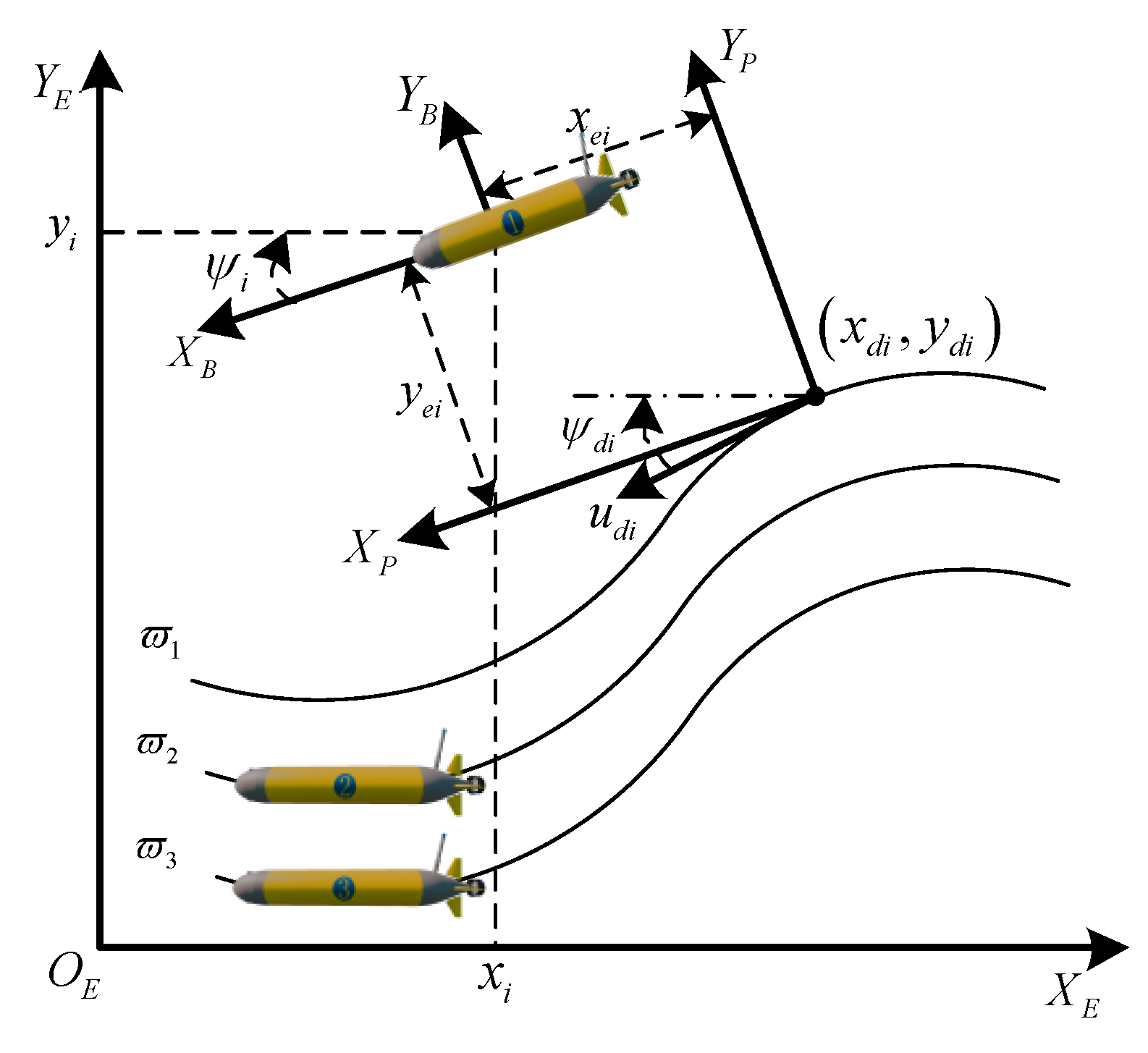
2.1. AUV Model

As shown in Figure 1, two types of reference frames, namely, the body-fixed frame and the earth-fixed frame, are widely used to describe AUV motions. Consider a cooperative system consisting of N under-actuated AUVs. Following the reference [41], the 3 degree-of-freedom (DOF) kinematics of the ith AUV is written as
η ˙ i = R ( ψ i ) v i ,
in which η i R 3 is a position state vector of coordinate ( x i , y i ) and heading angle ψ i of the ith AUV in the earth-fixed frame; v i R 3 is a velocity vector of surge velocity u i , sway velocity v i , and yaw angular velocity r i in the body-fixed frame; R ( ψ i ) is a 3-DOF rotation matrix defined as
R ( ψ i ) = [ cos ψ i sin ψ i 0 sin ψ i cos ψ i 0 0 0 1 ]
with properties as follows: R T ( ψ i ) R ( ψ i ) = I , R ( ψ i ) = 1 , and R ˙ ( ψ i ) = R ( ψ i ) S ( r i ) , where
S ( r i ) = [ 0 r i 0 r i 0 0 0 0 0 ] .
Under complex uncertainties including dynamic uncertainties and time-varying ocean currents, the dynamics is given by
( M ^ i + M ˜ i ) v ˙ i = ( C ^ i ( v i ) + C ˜ i ( v i ) ) v i ( D ^ i ( v i ) + D ˜ i ( v i ) ) v i + τ i + d i ,
in which τ i = [ τ u i , 0 , τ r i ] T R 3 is the control input vector, and d i = [ d u i , d v i , d r i ] T R 3 denotes ocean currents. The inertia matrix M ^ i R 3 × 3 , the coriolis matrix C ^ i ( v i ) R 3 × 3 , and the damping matrix D ^ i ( v i ) R 3 × 3 are given by
M ^ i = [ m ^ 11 0 0 0 m ^ 22 0 0 0 m ^ 33 ] , C ^ i ( v i ) = [ 0 0 m ^ 22 v i 0 0 m ^ 11 u i m ^ 22 v i m ^ 11 u i 0 ] ,
D ^ i ( v i ) = [ d ^ u + d ^ u u | u i | 0 0 0 d ^ v + d ^ v v | v i | 0 0 0 d ^ r + d ^ r r | r i | ] ,
in which M ^ i , C ^ i and D ^ i are the nominal values, and the corresponding parameter perturbations are defined as M ˜ i = M i M ^ i , C ˜ i = C i C ^ i , D ˜ i = D i D ^ i .

2.2. Problem Formualtion

Given a parameterized curved path without temporal constraints, a “virtual vehicle” ( x d i ( ϖ i ) , y d i ( ϖ i ) ) is regarded as the tracking target for the ith AUV. As depicted in Figure 1, a path reference frame is established where the axes are parallel to the surge velocity and sway velocity of the AUV. For an AUV located at the point ( x i , y i ) , the maneuvering errors between ( x i , y i ) and ( x d i ( ϖ i ) , y d i ( ϖ i ) ) in the path reference frame are
[ x e i y e i ] = [ cos ψ i sin ψ i sin ψ i cos ψ i ] T [ x d i ( ϖ i ) x i y d i ( ϖ i ) y i ] ,
in which x e i and y e i represent the along-maneuvering error and cross-maneuvering error, respectively. Taking time derivatives of x e i and y e i along (1), we get
[ x ˙ e i y ˙ e i ] = [ cos ( ψ d i ψ i ) 0 0 sin ( ψ d i ψ i ) ] [ u d i u d i ] [ u i v i ] + [ 0 ψ ˙ i ψ ˙ i 0 ] [ x e i y e i ] ,
in which ψ d i = atan 2 ( y ˙ d i , x ˙ d i ) ; And u d i > 0 is the virtual vehicle’s speed along the desired path, which can be expressed by
u d i = ϖ ˙ i x ˙ d i 2 + y ˙ d i 2 .
By combining with (4) and (7), the path-maneuvering error dynamics is rewritten as
{ x ˙ e i = y e i ψ ˙ i u i + u ¯ d i ϖ ˙ i cos ( ψ d i ψ i ) , y ˙ e i = x e i ψ ˙ i v i + u ¯ d i ϖ ˙ i sin ( ψ d i ψ i ) , ψ ˙ i = r i , m 11 u ˙ i = m 22 v i r i ( d u + d u u | u i | ) u i + d u i + τ u i , m 22 v ˙ i = m 11 u i r i ( d v + d v v | v i | ) v i + d v i + 0 , m 33 r ˙ i = ( m 11 m 22 ) u i v i ( d r + d r r | r i | ) r i + d r i + τ r i ,
in which u ¯ d i = x ˙ d i 2 + y ˙ d i 2 .
The maneuvering control objective is to propose a DCPMC approach for multiple AUVs with the dynamics (4) such that the assigned multiple parameterized paths can be synchronously tracked. Specifically, the objective is written as
{ lim t | x e i | 0 , lim t | y e i | 0 ,
and
lim t | ϖ i ϖ j | 0 ,
in which i = 1 , , N , j = 1 , , N , and i j .

3. Distributed Cooperative Path-Maneuvering Control

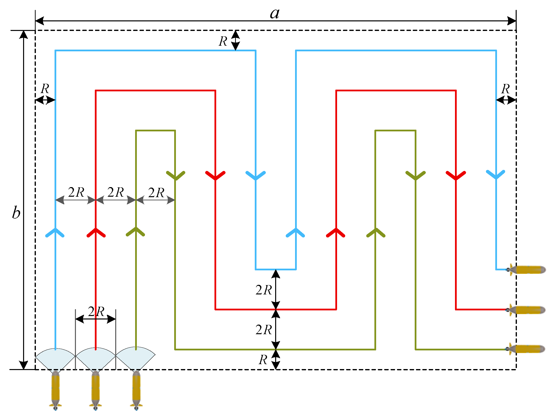
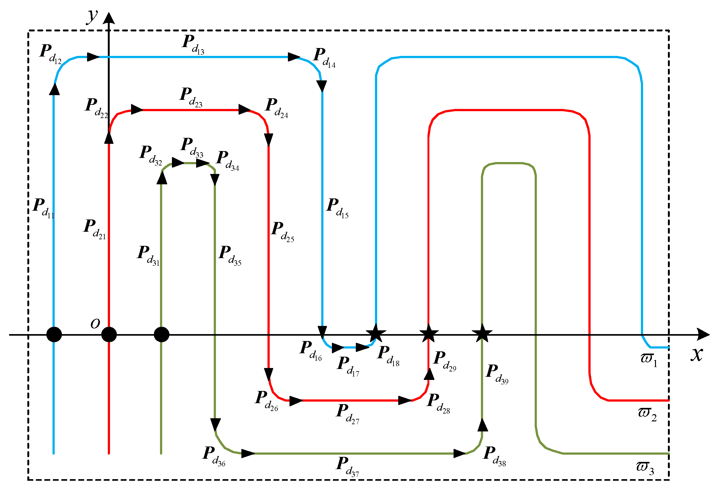
3.1. Coverage Path-Planning Design

To ensure the complete coverage for one region, a boustrophedon motion-based CPP is proposed and generates multiple desired paths. As shown in Figure 2, consider a search region a × b , together with the sensed area 2 R of an AUV, where a and b denote the area length and the area width, respectively. Our goal is to construct continuous curve paths and achieve complete coverage for this region.
Boustrophedon paths are firstly proposed for the CPP, where Boustrophedon means “the trajectory of the ox”. As an ox drags a plow in one region, it crosses the full length of the region in a straight line, turns around, and then traces a new straight line path adjacent to previous one. By repeating the aforementioned procedure, the ox achieves complete coverage for this region [42,43].
Remark 1.
Due to the vehicle maneuverability and minimum gyration radius constraints, boustrophedon paths mentioned above cannot be tracked directly. To this end, smooth boustrophedon paths are designed using trigonometric functions and deployed in Figure 3.
In what follows, the smooth paths are parameterized by time-dependent variables ϖ 1 , ϖ 2 , and ϖ 3 . Besides, each continuous curve path is composed of sub-path and has periodicity, where path variable starts at “the circle point” and ends at “the star point”.
By virtue of boustrophedon paths and trigonometric functions, the desired multiple paths for region-searching are expressed as
{ P d 1 ( ϖ 1 ) = P d 11 ( ϖ 1 ) P d 12 ( ϖ 1 ) P d 18 ( ϖ 1 ) , P d 2 ( ϖ 2 ) = P d 21 ( ϖ 2 ) P d 22 ( ϖ 2 ) P d 29 ( ϖ 2 ) , P d 3 ( ϖ 3 ) = P d 31 ( ϖ 3 ) P d 32 ( ϖ 3 ) P d 39 ( ϖ 3 ) ,
in which P d i denotes the parameterized curved path and composed of P d i i . To be specific, the complete paths can be described as
{ P d 11 = ( 2 R , ϖ 1 ) , ϖ 1 ( , ϖ 11 ] ; P d 12 = ( R R cos ( ( ϖ 1 ϖ 11 ) R 1 ) , ϖ 11 + R sin ( ( ϖ 1 ϖ 11 ) R 1 ) ) , ϖ 1 ( ϖ 11 , ϖ 12 ] ; P d 13 = ( ϖ 1 ϖ 12 R , α 11 b ) , ϖ 1 ( ϖ 12 , ϖ 13 ] ; P d 14 = ( 7 R + R sin ( ( ϖ 1 ϖ 13 ) R 1 ) ,   α 12 b + R cos ( ( ϖ 1 ϖ 13 ) R 1 ) ) , ϖ 1 ( ϖ 13 , ϖ 14 ] ; P d 15 = ( 8 R , ϖ 14 ϖ 1 + α 13 b ) , ϖ 1 ( ϖ 14 , ϖ 15 ] ; P d 16 = ( 8.5 R 0.5 R cos ( ( ϖ 1 ϖ 15 ) π ω 1 1 ) , 0.5 R sin ( ( ϖ 1 ϖ 15 ) π ω 1 1 ) ) , ϖ 1 ( ϖ 15 , ϖ 16 ] ; P d 17 = ( ϖ 1 ϖ 16 + 8.5 R , α 14 b ) , ϖ 1 ( ϖ 16 , ϖ 17 ] ; P d 18 = ( 9.5 R + 0.5 R sin ( ( ϖ 1 ϖ 17 ) π ω 1 1 ) , 0.5 R cos ( ( ϖ 1 ϖ 17 ) π ω 1 1 ) ) , ϖ 1 ( ϖ 17 , ϖ 18 ] ;
{ P d 21 = ( 0 , ϖ 2 ) , ϖ 2 ( , ϖ 21 ] ; P d 22 = ( R R cos ( ( ϖ 2 ϖ 21 ) π ω 2 1 ) ,   ϖ 21 + R sin ( ( ϖ 2 ϖ 21 ) π ω 2 1 ) ) , ϖ 2 ( ϖ 21 , ϖ 22 ] ; P d 23 = ( ϖ 2 ϖ 22 + R , α 21 b ) , ϖ 2 ( ϖ 22 , ϖ 23 ] ; P d 24 = ( 5 R + R sin ( ( ϖ 2 ϖ 23 ) π ω 2 1 ) ,   α 22 b R cos ( ( ϖ 2 ϖ 23 ) π ω 2 1 ) ) , ϖ 2 ( ϖ 23 , ϖ 24 ] ; P d 25 = ( 6 R , ϖ 24 ϖ 2 + α 23 b ) , ϖ 2 ( ϖ 24 , ϖ 25 ] ; P d 26 = ( 7 R R cos ( ( ϖ 2 ϖ 25 ) π ω 2 1 ) , α 24 b R sin ( ( ϖ 2 ϖ 25 ) π ω 2 1 ) ) , ϖ 2 ( ϖ 25 , ϖ 26 ] ; P d 27 = ( ϖ 2 ϖ 26 + 7 R , α 25 b ) , ϖ 2 ( ϖ 26 , ϖ 27 ] ; P d 28 = ( 11 R + R sin ( ( ϖ 2 ϖ 27 ) π ω 1 1 ) , α 26 b R cos ( ( ϖ 2 ϖ 27 ) π ω 1 1 ) ) , ϖ 2 ( ϖ 27 , ϖ 28 ] ; P d 29 = ( 12 R , ϖ 2 ϖ 28 α 27 b ) , ϖ 2 ( ϖ 28 , ϖ 29 ] ;
and
{ P d 31 = ( 2 R , ϖ 3 ) , ϖ 3 ( , ϖ 31 ] ; P d 32 = ( 2.5 R 0.5 R cos ( ( ϖ 3 ϖ 31 ) π ω 3 1 ) , ϖ 31 + 0.5 R sin ( ( ϖ 3 ϖ 31 ) π ω 3 1 ) ) , ϖ 3 ( ϖ 31 , ϖ 32 ] ; P d 33 = ( ϖ 3 ϖ 32 + 2.5 R , α 31 b ) , ϖ 3 ( ϖ 32 , ϖ 33 ] ; P d 34 = ( 3.5 R + 0.5 R sin ( ( ϖ 3 ϖ 33 ) π ω 3 1 ) , α 32 b 0.5 R cos ( ( ϖ 3 ϖ 33 ) π ω 3 1 ) ) , ϖ 3 ( ϖ 33 , ϖ 34 ] ; P d 35 = ( 4 R , ϖ 34 ϖ 3 + α 33 b ) , ϖ 3 ( ϖ 34 , ϖ 35 ] ; P d 36 = ( 5 R R cos ( ( ϖ 3 ϖ 35 ) R 1 ) , α 34 b R sin ( ( ϖ 3 ϖ 35 ) R 1 ) ) , ϖ 3 ( ϖ 35 , ϖ 36 ] ; P d 37 = ( ϖ 3 ϖ 36 + 5 R , α 35 b ) , ϖ 3 ( ϖ 36 , ϖ 37 ] ; P d 38 = ( 13 R R sin ( ( ϖ 3 ϖ 37 ) R 1 ) , α 36 b R cos ( ( ϖ 3 ϖ 37 ) R 1 ) ) , ϖ 3 ( ϖ 37 , ϖ 38 ] ; P d 39 = ( 14 R , ϖ 3 ϖ 38 α 37 b ) , ϖ 3 ( ϖ 38 , ϖ 39 ] ;
in which ϖ 1 i , ϖ 2 i , and ϖ 3 i are sub-path variables. α 1 i , α 2 i , and α 3 i are design parameters with respect to the special region. ω 1 , ω 2 , and ω 3 are path parameters without temporal constraints.
Remark 2.
Based on the practical considerations, three AUVs are widely applied to varieties of missions, and because of this, three boustrophedon paths are constructed and tracked in this article.

3.2. Individual Path-Maneuvering Control Design

In practice, dynamic uncertainties and/or ocean currents have an adverse impact on path-maneuvering performance. It is highly desirable to develop robust control laws for under-actuated AUVs. To this end, the dynamics (4) can be rewritten as
{ m ^ 11 u ˙ i = m ^ 22 v i r i φ 1 i T ζ 1 i + δ 1 i + τ u i , m ^ 22 v ˙ i = m ^ 11 u i r i φ 2 i T ζ 2 i + δ 2 i + 0 , m ^ 33 r ˙ i = ( m ^ 11 m ^ 22 ) u i v i φ 3 i T ζ 3 i + δ 3 i + τ r i ,
in which δ 1 i , δ 2 i , and δ 3 i denote nonlinear dynamics determined by
{ δ 1 i = d u i m ˜ 11 u ˙ i + m ˜ 22 v i r i , δ 2 i = d v i m ˜ 22 v ˙ i m ˜ 11 u i r i , δ 3 i = d r i m ˜ 33 r ˙ i + ( m ˜ 11 m ˜ 22 ) u i v i ,
with φ 1 i = [ u i | u i | , u i ] T , φ 2 i = [ v i | v i | , v i ] T , φ 3 i = [ r i | r i | , r i ] T , ζ 1 i = [ d u u , d u ] T , ζ 2 i = [ d v v , d v ] T , and ζ 3 i = [ d r r , d r ] T .
In order to achieve (10), virtual control laws are designed at the kinematic hierarchy, and then adaptive sliding controllers are designed at the dynamic hierarchy. In the following, we define u e i = u i α u i , r e i = r i α r i , ψ e i = ψ d i ψ i , ϖ ˙ i = v s i ( ϖ i ) υ i , ζ ˜ 1 i = ζ ^ 1 i ζ 1 i , and ζ ˜ 3 i = ζ ^ 3 i ζ 3 i , in which α u i and α r i are virtual control variables; v s i is a distributed speed assignment and υ i is a consensus protocol variable to accomplish synchronized motions; ζ ^ 1 i and ζ ^ 3 i are the estimations for uncertainties.
In this context, the path-maneuvering error dynamics for kinematics is reformulated by
{ x ˙ e i = y e i ψ ˙ i u i + u ¯ d i ( v s i υ i ) cos ψ e i , y ˙ e i = x e i ψ ˙ i v i + u ¯ d i ( v s i υ i ) sin ψ e i , ψ ˙ e i = ψ ˙ d i r i .
Consider the following Lyapunov candidate function
V 1 = k 1 ( 1 cos ψ e i ) + 1 2 ( x e i 2 + y e i 2 ) ,
in which k 1 > 0 .
Differentiating V 1 along the error dynamics (18) yields
V ˙ 1 = x e i ( y e i ψ ˙ i u i + u ¯ d i ( v s i υ i ) cos ψ e i ) + y e i ( x e i ψ ˙ i   v i + u ¯ d i ( v s i υ i ) sin ψ e i ) k 1 sin ψ e i ( ψ ˙ d i r i ) = x e i ( u ¯ d i ( v s i υ i ) cos ψ e i u i ) y e i v i + sin ψ e i ( u ¯ d i   ( v s i υ i ) y e i k 1 ( ψ ˙ d i r i ) ) .
Then, choosing the virtual control laws α u i and α r i as
{ α u i = u ¯ d i ϖ ˙ i cos ψ e i + k 2 x e i + u ¯ d i υ i , α r i = ψ ˙ d i + 1 k 2 u ¯ d i ϖ ˙ i y e i + k 1 u ¯ d i ϖ ˙ i sin ψ e i ,
in which k 2 > 0 .
Submitting (21) into (20), there is
V ˙ 1 = k 1 2 u ¯ d i ϖ ˙ i sin 2 ψ e i k 2 x e i 2 + u ¯ d i υ i x e i u e i x e i k 1 r e i sin ψ e i v i y e i .
Note that α u i and α r i could not be directly applied in practice. In this context, consider the Lyapunov candidate function
V 2 = V 1 + 1 2 ( u e i 2 + r e i 2 ) .
Differentiating V 2 along u e i and r e i , we have
V ˙ 2 = k 1 2 u ¯ d i ϖ ˙ i sin 2 ψ e i k 2 x e i 2 + u ¯ d i υ i x e i k 1 r e i sin ψ e i u e i x e i v i y e i + u e i ( u ˙ i u ˙ d i ) + r e i ( r ˙ i r ˙ d i ) .
By combining with sliding mode and adaptive technique, we design the maneuvering control laws for surge and yaw motions as follows
{ τ u i = m ^ 11 ( α ˙ u i k 3 u e i + x e i η 1 sgn ( u e i ) ) + φ 1 i T ζ ^ 1 i m ^ 22 v i r i , τ r i = m ^ 33 ( α ˙ r i k 4 r e i + k 1 sin ψ e i x e i η 2 sgn ( r e i ) ) + φ 3 i T ζ ^ 3 i ( m ^ 11 m ^ 22 ) u i v i ,
with update laws
{ ζ ^ ˙ 1 i = λ 1 u e i φ 1 i , ζ ^ ˙ 3 i = λ 3 r e i φ 3 i ,
in which k 3 , k 4 , η 1 , η 2 , λ 1 , and λ 3 are positive constants, and sgn ( u e i ) is the switching function given by
sgn ( u e i ) = { 1 ,   u e i > 0 ; 0 ,   u e i = 0 ; 1 ,   u e i < 0 .
In addition, sgn ( r e i ) has the similar structure with (27).
Remark 3.
To overcome chattering of the discontinuous switch function, a saturation function is employed by
sat ( u e i ; μ , σ ) = { sgn ( u e i ) ,   | u e i | > μ ; sig σ ( u e i ) μ σ ,   | u e i | μ ;
with μ > 0 and 0 < σ < 1 .
Substituting the control laws (25) into (24), and using dynamics (16), we have
V ˙ 2 = k 1 2 u ¯ d i ϖ ˙ i sin 2 ψ e i k 2 x e i 2 + u ¯ d i υ i x e i u e i x e i k 1 r e i sin ψ e i v i y e i + u e i ( δ 1 i / m ^ 11 + x e i η 1 sgn ( u e i ) φ 1 i T ζ 1 i / m ^ 11 + φ 1 i T ζ ^ 1 i / m ^ 11 k 4 u e i ) + r e i ( δ 3 i / m ^ 33 k 5 r e i + k 1 sin ψ e i η 2 sgn ( r e i ) φ 3 i T ζ 3 i / m ^ 33 + φ 3 i T ζ ^ 3 i / m ^ 33 ) = k 1 2 u ¯ d i ϖ ˙ i sin 2 ψ e i k 2 x e i 2 + u ¯ d i υ i x e i k 3 u e i 2 k 4 r e i 2 v i y e i + u e i ( δ 1 i / m ^ 11 η 1 sgn ( u e i ) + φ 1 i T ζ ˜ 1 i / m ^ 11 ) + r e i ( δ 3 i / m ^ 33 η 2 sgn ( r e i ) + φ 3 i T ζ ˜ 3 i / m ^ 33 ) .
The key result on individual path-following control is summarized as follows.
Theorem 1.
Consider the dynamics (9) and the control laws (25) with (26). Then, error signals u e i , r e i , ψ e i , x e i , and y e i asymptotically converge to zero.
Proof of Theorem 1.
Consider the Lyapunov candidate function
V 3 = V 2 + 1 2 λ 1 m ^ 11 ζ ˜ 1 i T ζ ˜ 1 i + 1 2 λ 3 m ^ 33 ζ ˜ 3 i T ζ ˜ 3 i ,
whose time derivative is
V ˙ 3 = k 1 2 u ¯ d i ϖ ˙ i sin 2 ψ e i k 2 x e i 2 + u ¯ d i υ i x e i k 3 u e i 2 k 4 r e i 2 + u e i ( δ 1 i / m ^ 11 η 1 sgn ( u e i ) ) v i y e i + r e i ( δ 3 i / m ^ 33 η 2 sgn ( r e i ) ) + u e i φ 1 i T ζ ˜ 1 i / m ^ 11 + r e i φ 3 i T ζ ˜ 3 i / m ^ 33 + ζ ˜ ˙ 1 i ζ ˜ 1 i / λ 1 m ^ 11 + ζ ˜ ˙ 3 i ζ ˜ 3 i / λ 3 m ^ 33 .
Using the fact that v i y e i = ε v i y e i + ( 1 ε ) v i y e i and the update laws (26), (31) becomes
V ˙ 3 = k 1 2 u ¯ d i ϖ ˙ i sin 2 ψ e i k 2 x e i 2 + u ¯ d i υ i x e i k 3 u e i 2 k 4 r e i 2 + u e i ( δ 1 i / m ^ 11   ε v i y e i / u e i η 1 sgn ( u e i ) ) + r e i ( δ 3 i / m ^ 33 η 2 sgn ( r e i ) ( 1 ε ) v i y e i / r e i ) ,
in which 0 < ε < 1 .
By the aid of the boundedness of the sway velocity v i , i.e., | v i ( t ) | 2 ϑ / d v + | v i ( t 0 ) | e 0.5 d v ( t t 0 ) mentioned in [17], we have the following inequality
{ | δ 1 i / m ^ 11 ε v i y e i / u e i | η 1 , | δ 3 i / m ^ 33 ( 1 ε ) v i y e i / r e i | η 2 .
Note that synchronization variable υ i is zero since path parameter synchronization is not considered in the IPMC design. Then, substituting (33) into (32), there is
V ˙ 3 < 0 ,   [ u e i , r e i , ψ e i , ζ ˜ 1 i , ζ ˜ 3 i , x e i , y e i ] T 0 ,
which implies that error signals u e i , r e i , ψ e i , x e i , and y e i asymptotically converge to zero. Thus, the proof is completed. □

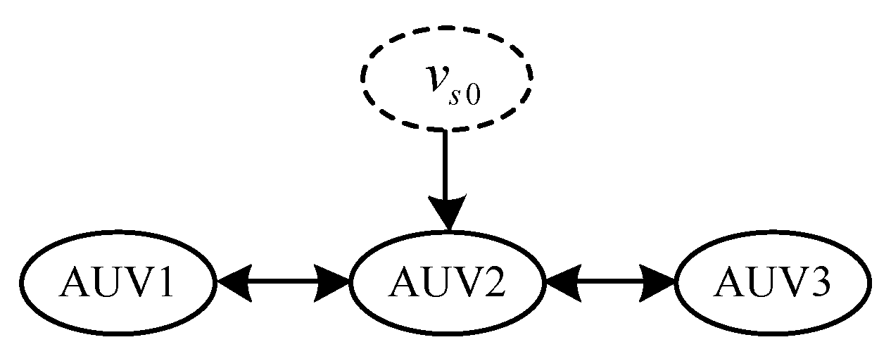
3.3. Path Parameter Synchronization Design

Consider the communication topology described by a graph G = ( ο , ε ) with the set of nodes ο = { n 1 , , n N } and the set of edges ε = { ( n i , n j ) ο × ο } . In this graph, a node represents an AUV and the element ( n i , n j ) describes information interactions from one node to another. A ( G ) = [ a i j ] R N × N denotes an adjacency matrix, where a i j = 1 if ( n i , n j ) ε ; Otherwise, a i j = 0 , and the Laplacian matrix L ( G ) = [ l i j ] R N × N is introduced with
l i j = { a i j ,   if   i j   and   j N i ; j N i a i j ,   if   i = j ; 0 ,   otherwise
It is worth noting that L ( G ) in the connected graph is symmetric and positive semi-definite. In addition, the corresponding eigenvector with minimum eigenvalue of zero is I = [ 1 , , 1 ] T , thus resulting in L ( G ) I = 0 N .
Consider that parts of the nodes are able to obtain the speed assignment. The accessorial matrix D ( G ) = diag { d 1 , , d N } is proposed, where d i = 1 represents that the node can get information from the speed assignment and d i = 0 represents that it cannot. In addition, the symmetric and positive definite matrix H ( G ) = L ( G ) + D ( G ) is satisfied for the undirected connected graph.
The key result on the distributed signal observer is collected as follows.
Theorem 2.
Consider that only the parts of AUVs receive the speed assignment and the distributed signal observer given by
v ^ ˙ s i = j = 0 N a i j ( v ^ s i v ^ s j ) ,
in which v ^ s 0 = v s 0 is a desired speed assignment and satisfies v ˙ s 0 = 0 . Then, lim t | v ^ s i | v s 0 , can be guaranteed.
Proof of Theorem 2.
Define observation error as
v ˜ s i = v ^ s i v s 0 .
Taking time derivatives along (36) yields
v ˜ ˙ s i = v ^ ˙ s i v ˙ s 0 = j = 0 N a i j [ ( v ^ s i v ^ s ) ( v ^ s j v ^ s ) ] = j = 0 N a i j ( v ˜ s i v ˜ s j ) .
Defining v ˜ s = [ v ˜ s i ] R N × 1 , we have
v ˜ ˙ s = ( H ( G ) I ) v ˜ s .
Consider the Lyapunov candidate function V s = 1 / 2 v ˜ s T v ˜ s and differentiating V s along (39) yields
V ˙ s = v ˜ s T ( H ( G ) I ) v ˜ s 0 ,
which implies that observation error v ˜ s i can converge to zero. This proof is complete. □
Furthermore, based on neighbors’ parameter information, we define the following coordination errors
e i = j = 1 N i a i j ( ϖ i ϖ j ) ,
and design the consensus protocol as
υ i = ξ i e i ξ i u ¯ d i x e i ,
in which ξ i > 0 .
In vector form, (42) can be presented as
{ ϖ ˙ = v ^ s ( ϖ ) υ , e = L ( G ) ϖ ,
here ϖ = [ ϖ i ] R N × 1 , v ^ s = [ v ^ s i ] R N × 1 , υ = [ υ i ] R N × 1 , and e = [ e i ] R N × 1 .
Computing the time derivative of e and using L ( G ) I = 0 N , we obtain
e ˙ = L ˙ ( G ) ϖ + L ( G ) ( v ^ s ( ϖ ) υ ) = L ( G ) υ .
Eventually, the path-maneuvering error dynamics (9) is rewritten as
{ x ˙ e i = y e i ψ ˙ i u i + u ¯ d i ( v s υ i ) cos ψ e i , y ˙ e i = x e i ψ ˙ i v i + u ¯ d i ( v s υ i ) sin ψ e i , ψ ˙ e i = ψ ˙ d i r i , m 11 u ˙ i = m 22 v i r i ( d u + d u u | u i | ) u i + d u i + τ u i , m 22 v ˙ i = m 11 u i r i ( d v + d v v | v i | ) v i + d v i + 0 , m 33 r ˙ i = ( m 11 m 22 ) u i v i ( d r + d r r | r i | ) r i + d r i + τ r i , e ˙ = L ( G ) υ .

3.4. Stability Analysis

The following theorem exhibits the stability result of the proposed DCPMC approach.
Theorem 3.
Consider a cluster of AUVs with dynamics (4), the control laws (25), and the consensus protocol (42). Then, all error signals in the closed-loop system are GAS.
Proof of Theorem 3.
Consider the following Lyapunov candidate function
V = i = 1 N { 1 2 ( x e i 2 + y e i 2 + u e i 2 + r e i 2 ) + k 2 ( 1 cos ψ e i ) + 1 2 λ 1 m ^ 11 ζ ˜ 1 T ζ ˜ 1 + 1 2 λ 3 m ^ 33 ζ ˜ 3 T ζ ˜ 3 } + 1 2 e T P e .
Using Lemma 1 in [39] yields that ϖ T L ( G ) ϖ = e T P e , where P is a positive definite matrix. In this context, (46) becomes
V = i = 1 N { 1 2 ( x e i 2 + y e i 2 + u e i 2 + r e i 2 ) + k 2 ( 1 cos ψ e i ) + 1 2 λ 1 m ^ 11 ζ ˜ 1 T ζ ˜ 1 + 1 2 λ 3 m ^ 33 ζ ˜ 3 T ζ ˜ 3 } + 1 2 ϖ T L ( G ) ϖ ,
whose derivative along (45) is
V ˙ = i = 1 N { k 1 2 u ¯ d i ϖ ˙ i sin 2 ψ e i k 2 x e i 2 k 3 u e i 2 k 4 r e i 2 + u e i ( δ 1 i / m ^ 11   ε v i y e i / u e i + r e i ( δ 3 i / m ^ 33 η 2 sgn ( r e i ) ( 1 ε ) v i y e i / r e i ) } + i = 1 N { u ¯ d i υ i x e i ϖ i T L ( G ) υ i } i = 1 N { k 1 2 u ¯ d i ϖ ˙ i sin 2 ψ e i k 2 x e i 2 k 3 u e i 2 k 4 r e i 2 } λ min ( ξ ) γ 2 ,
in which ξ = diag { ξ 1 , , ξ N } , γ = e + u ¯ d x e , x e = [ x e i ] R N × 1 , and u ¯ d = diag { u ¯ d 1 , , u ¯ d N } . By straightforward derivation [44], one can conclude that all error signals are GAS. This concludes the proof. □
Remark 4.
By virtue of the inequality x T S y m ( L ( G ) ) x ξ s ( S y m ( L ( G ) ) ) x 1 N 1 N T x / N 2 and S y m ( L ( G ) ) = ( L ( G ) + L ( G ) T ) / 2 in [45], one can conclude that e T P e ξ s ϖ i = 1 N ϖ i / N 2 and lim t | ϖ i ϖ j | 0 .

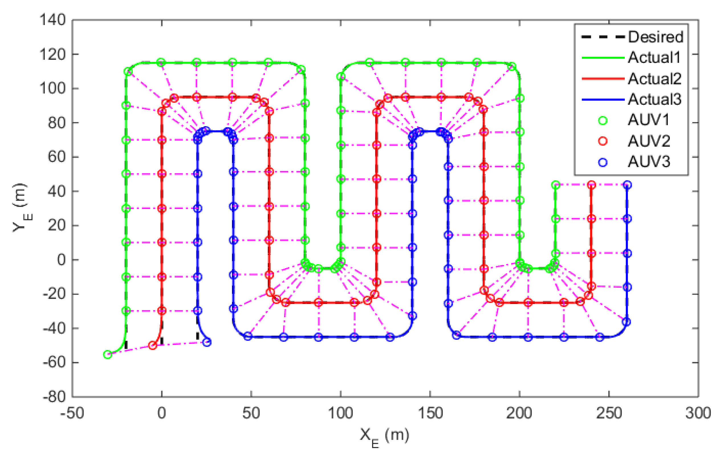
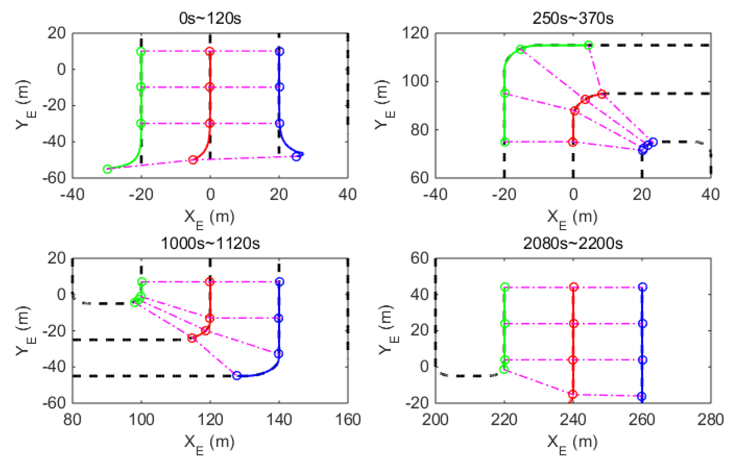
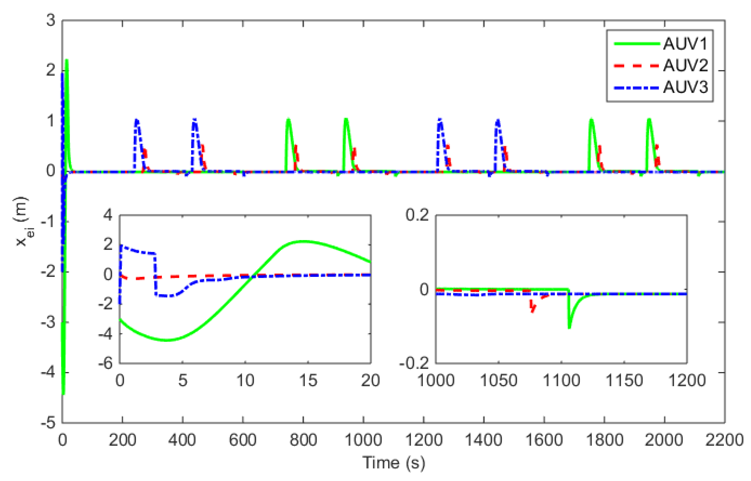
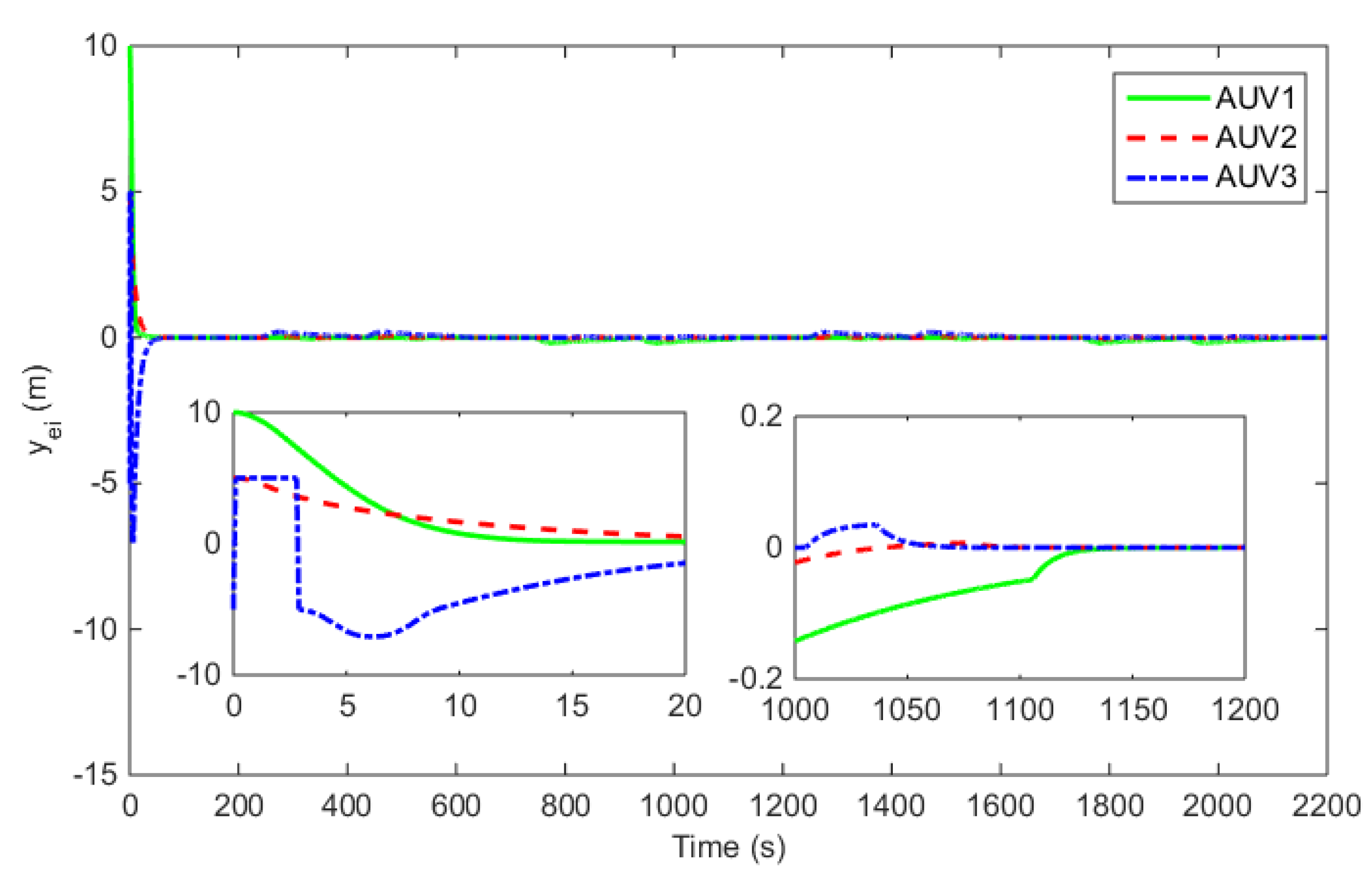
4. Simulation Studies

To evaluate the proposed DCPMC approach, simulation studies are given in this section. The weight of the AUV called WL-II is 45 kg and the length is 1.46 m. Besides, model parameters are illustrated in Table 1 [46].
Let the information topology among the three AUVs be described by Figure 4, where only AUV 2 can receive the speed signal. Consider the special region with a = 180 m , b = 300 m , and the sensed area of an AUV with R = 10 m . The desired coverage paths are generated by (13), (14) and (15), where path parameters are illustrated in Table 2.
For the sake of simulation setup, dynamic uncertainties and ocean currents are assumed as follows: m ˜ 11 = 0.1 m ^ 11 , m ˜ 22 = 0.1 m ^ 22 , m ˜ 33 = 0.15 m ^ 33 , d u i = ϑ 1 κ 1 , d v i = ϑ 2 κ 2 , and d r i = ϑ 3 κ 3 , where κ i > 0 are constants and ϑ i are zero-mean Gaussian white noise processes [47,48]. The initial conditions of three AUVs are set as follows: η 1 ( 0 ) = [ 30 , 55 , π / 6 ] T , η 2 ( 0 ) = [ 5 , 50 , π / 3 ] T , η 3 ( 0 ) = [ 25 , 48 , π / 2 ] T , v 1 ( 0 ) = [ 0 , 0 , 0 ] T , v 2 ( 0 ) = [ 0 , 0 , 0 ] T , and v 3 ( 0 ) = [ 0 , 0 , 0 ] T .
As shown in Figure 5, three AUVs converge to the desired paths generated by the CPP design and keep a synchronized formation simultaneously. Besides, taking readability into consideration, Figure 6 shows the snapshots of three AUVs in different time periods. From Figure 7 and Figure 8, it is observed that along-maneuvering and cross-maneuvering errors can converge to the origin in a short time. The small chattering existing in tracking errors is caused by the switching of the straight line and the curve. The path parameter variables of three AUVs are given in Figure 9 and almost synchronized. Figure 10 and Figure 11 show the AUV heading angles, surge and yaw angular velocities, respectively. Note that the desired paths are designed using piecewise function, thereby leading to slight chattering for control inputs in Figure 12. The observation results on speed signals are given in Figure 13, which can exhibit excellent observation performance. Furthermore, comparisons on maneuvering errors and velocity signals of individual AUV are given in Figure 14. It is apparent that the proposed approach has better maneuvering performance than the backsteeping-based approach ( η i = 0 , i = 1 , 2 ), thus contributing to less abrasion of actuators.

5. Conclusions

In this article, a DCPMC approach was developed for a cluster of under-actuated AUVs under undirected communication topology. By the aid of smooth boustrophedon paths, the CPP is designed for the region-searching, where multiple parameterized paths are generated and used to be tracked. Within the dynamics controllers, adaptive sliding mode techniques are used to design maneuvering control laws, which can drive vehicles to track the assigned paths despite the existence of dynamic uncertainties and ocean currents. Besides, the consensus protocol with distributed signal observer is developed for path parameter synchronization, thus contributing to the desired formation configuration. Rigorous theoretical derivation and proof have exhibited that the resulting closed-loop signals are GAS, and simulation results have illustrated the effectiveness of the DCPMC approach.

Author Contributions

Conceptualization, T.C. and X.Q.; methodology, X.Q.; software, X.Q.; validation, T.C., X.L. and Z.Z.; formal analysis, Z.Z.; investigation, T.C.; resources, X.Q.; data curation, X.Q.; writing—original draft preparation, X.Q.; writing—review and editing, X.Q.; visualization, Z.Z.; supervision, T.C.; project administration, X.L.; funding acquisition, X.L. All authors have read and agreed to the published version of the manuscript.

Funding

This research was funded by the National Natural Science Foundation of China (under Grant 51809060 and Grant 51879023), the Maritime Defence Technologies Innovation Foundation (under Grant JJ-2020-701-02 and Grant JJ-2020-719-06), the LiaoNing Revitalization Talents Program (under Grant XLYC1907180), the Liaoning Provincial Natural Science Foundation of China (under Grant 2019-KF-01-16), and the Innovation Project for Dalian Maritime University Double First-Class Construction (under Grant BSCXXM024).

Institutional Review Board Statement

Not applicable.

Informed Consent Statement

Not applicable.

Data Availability Statement

Not applicable.

Conflicts of Interest

The authors declare no conflict of interest.

References

  1. Bays, M.J.; Shende, A.; Seilwell, J.J. Theory and experimental results for the multiple aspect coverage problem. Ocean Eng. 2012, 54, 51–60. [Google Scholar] [CrossRef]
  2. Lapierre, L.; Zapata, R.; Lepinay, P. Karst exploration: Unconstrained attitude dynamic control for an AUV. Ocean Eng. 2021, 219, 108321. [Google Scholar] [CrossRef]
  3. Li, Y.; Li, Y.; Wu, Q. Design for three-dimensional stabilization control of underactuated autonomous underwater vehicles. Ocean Eng. 2018, 150, 327–336. [Google Scholar] [CrossRef]
  4. Kim, J.; Joe, H.; Yu, S. Time-Delay Controller Design for Position Control of Autonomous Underwater Vehicle Under Disturbances. Trans. Ind. Electron. 2016, 63, 1052–1061. [Google Scholar] [CrossRef]
  5. Fossen, T.I.; Pettersen, K.Y.; Galeazzi, R. Line-of-sight path following for dubins paths with adaptive sideslip compensation of drift forces. IEEE Trans. Control Syst. Technol. 2015, 23, 820–827. [Google Scholar] [CrossRef] [Green Version]
  6. Wynn, R.B.; Huvenne, V.A.I.; Le, B. Autonomous underwater vehicles: Their past, present and future contributions to the advancement of marine geoscience. Mar. Geol. 2014, 352, 451–468. [Google Scholar] [CrossRef] [Green Version]
  7. Qiao, L.; Zhang, W. Adaptive non-singular integral terminal sliding mode tracking control for autonomous underwater vehicles. IET Control Theory Appl. 2017, 11, 1293–1306. [Google Scholar] [CrossRef]
  8. Wu, D.; Liao, Y.; Hu, C. An enhanced fuzzy control strategy for low-level thrusters in marine dynamic positioning systems based on chaotic random distribution harmony search. Int. J. Fuzzy Syst. 2020. [Google Scholar] [CrossRef]
  9. Huang, Y.; Wu, D.; Yin, Z. Design of UDE-based dynamic surface control for dynamic positioning of vessels with complex disturbances and input constraints. Ocean Eng. 2021, 220, 108487. [Google Scholar] [CrossRef]
  10. Qiao, L.; Zhang, W. Trajectory tracking control of AUVs via adaptive fast nonsingular integral terminal sliding mode control. IEEE Trans. Ind. Inform. 2020, 16, 1248–1258. [Google Scholar] [CrossRef]
  11. Qiao, L.; Zhang, W. Adaptive second-order fast nonsingular terminal sliding mode tracking control for fully actuated autonomous underwater vehicles. IEEE J. Ocean. Eng. 2019, 44, 363–385. [Google Scholar] [CrossRef]
  12. Wang, N.; Sun, Z.; Jiao, Y. Surge-Heading Guidance Based Finite-Time Path-Following of Underactuated Marine Vehicles. IEEE Trans. Veh. Technol. 2019, 68, 8523–8532. [Google Scholar] [CrossRef]
  13. Liang, X.; Qu, X.; Hou, Y. Finite-time Unknown Observer Based Coordinated Path-Following Control of Unmanned Underwater Vehicles. J. Frankl. Inst. 2021. [Google Scholar] [CrossRef]
  14. Liang, X.; Qu, X.; Wang, N. Swarm velocity guidance based distributed finite-time coordinated path-following for uncertain under-actuated autonomous surface vehicles. ISA Trans. 2021. [Google Scholar] [CrossRef]
  15. Liang, X.; Qu, X.; Wang, N. Swarm control with collision avoidance for multiple underactuated surface vehicles. Ocean Eng. 2019, 191, 106516. [Google Scholar] [CrossRef]
  16. Qu, X.; Liang, X.; Hou, Y. Path-following control of unmanned surface vehicles with unknown dynamics and unmeasured velocities. J. Mar. Sci. Technol. 2020. [Google Scholar] [CrossRef]
  17. Qu, X.; Liang, X.; Hou, Y. Fuzzy State Observer Based Cooperative Path-Following Control of Autonomous Underwater Vehicles with Unknown Dynamics and Ocean Disturbances. Int. J. Fuzzy Syst. 2020. [Google Scholar] [CrossRef]
  18. Liang, X.; Qu, X.; Wang, N. A Novel Distributed and Self-Organized Swarm Control Framework for Underactuated Unmanned Marine Vehicles. IEEE Access 2019, 7, 112703–112712. [Google Scholar] [CrossRef]
  19. Hinostroza, M.A.; Xu, H.; Guedes Soares, C. Cooperative operation of autonomous surface vehicles for maintaining formation in complex marine environment. Ocean Eng. 2019, 183, 132–154. [Google Scholar] [CrossRef]
  20. Loria, A.; Dasdemir, J.; Jarquin, N.A. Leader-Follower formation and tracking control of mobile robots along straight paths. IEEE Trans. Control Syst. Technol. 2016, 24, 727–732. [Google Scholar] [CrossRef] [Green Version]
  21. Ren, W. Consensus strategies for cooperative control of vehicle formations. IET Control Theory Appl. 2007, 1, 505–512. [Google Scholar] [CrossRef]
  22. Tsai, C.C.; Wu, H.L.; Tai, F. Distributed Consensus Formation Control with Collision and Obstacle Avoidance for Uncertain Networked Omnidirectional Multi-Robot Systems Using Fuzzy Wavelet Neural Networks. Int. J. Fuzzy Syst. 2017, 19, 1375–1391. [Google Scholar] [CrossRef]
  23. Lee, G.; Chwa, D. Decentralized behavior-based formation control of multiple robots considering obstacle avoidance. Intell. Serv. Robot. 2018, 11, 127–138. [Google Scholar] [CrossRef]
  24. Park, B.S.; Yoo, S.J. Adaptive-observer-based formation tracking of networked uncertain underactuated surface vessels with connectivity preservation and collision avoidance. J. Frankl. Inst. 2019, 356, 7947–7966. [Google Scholar] [CrossRef]
  25. Fan, J.; Liao, Y.; Li, Y. Formation Control of Multiple Unmanned Surface Vehicles Using the Adaptive Null-Space-Based Behavioral Method. IEEE Access 2019, 7, 87647–87657. [Google Scholar] [CrossRef]
  26. Liu, L.; Wang, D.; Peng, Z. Cooperative Path Following Ring-Networked Under-Actuated Autonomous Surface Vehicles: Algorithms and Experimental Results. IEEE Trans. Cybern. 2020, 50, 1519–1529. [Google Scholar] [CrossRef] [PubMed]
  27. Liu, L.; Wang, D.; Peng, Z. Coordinated path following of multiple underacutated marine surface vehicles along one curve. ISA Trans. 2016, 64, 258–268. [Google Scholar] [CrossRef]
  28. Almeida, J.; Silvestre, C.; Pascoal, A. Cooperative control of multiple surface vessels in the presence of ocean currents and parametric model uncertainty. Int. J. Robust Nonlinear Control 2010, 20, 1549–1565. [Google Scholar] [CrossRef]
  29. Qu, X.; Liang, X.; Hou, Y. Finite-time sideslip observer-based synchronized path-following control of multiple unmanned underwater vehicles. Ocean Eng. 2020, 217, 107941. [Google Scholar] [CrossRef]
  30. Almeida, J.; Silvestre, C.; Pascoal, A. Cooperative control of multiple surface vessels with discrete-time periodic communications. Int. J. Robust Nonlinear Control 2011, 22, 398–419. [Google Scholar] [CrossRef]
  31. Bibuli, M.; Bruzzone, G.; Caccia, M. Swarm based path-following for cooperative unmanned surface vehicles. J. Eng. Marit. Environ. 2014, 228, 192–207. [Google Scholar] [CrossRef]
  32. Wang, H.; Wang, D.; Peng, Z. Adaptive dynamic surface control for cooperative path following of underactuated marine surface vehicles via fast learning. IET Control Theory Appl. 2013, 7, 1888–1898. [Google Scholar]
  33. Xiang, X.; Liu, C.; Lapierre, L. Synchronized path following control of multiple homogenous underactuated UUVs. J. Syst. Sci. Complex. 2012, 25, 71–89. [Google Scholar] [CrossRef]
  34. Chen, Y.; Wei, P. Coordinated Adaptive Control for Coordinated Path-following Surface Vessels with a Time-invariant Orbital Velocity. IEEE/CAA J. Autom. Sin. 2014, 1, 337–346. [Google Scholar]
  35. Liang, X.; Qu, X.; Hou, Y. Distributed coordinated tracking control of multiple unmanned surface vehicles under complex marine environments. Ocean Eng. 2020, 205, 107328. [Google Scholar] [CrossRef]
  36. Kim, H.; Kim, S.H.; Jeon, M. A study on path optimization method of an unmanned surface vehicle under environmental loads using genetic algorithm. Ocean Eng. 2017, 142, 616–624. [Google Scholar] [CrossRef]
  37. Wu, D.; Ma, Z.; Li, A. Identification for fractional order rational models based on particle swarm optimization. Int. J. Comput. Appl. Technol. 2011, 41, 53–59. [Google Scholar] [CrossRef]
  38. Sang, H.; You, Y.; Sun, X. The hybrid path planning algorithm based on improved A* and artificial potential field for unmanned surface vehicle formations. Ocean Eng. 2021, 223, 108709. [Google Scholar] [CrossRef]
  39. Kawabata, K.; Ma, L.; Xue, J. A path generation for automated vehicle based on Bezier curve and via-points. Robot. Auton. Syst. 2015, 74, 243–252. [Google Scholar] [CrossRef]
  40. Wang, N.; Jin, X.; Er, M.J. A multilayer path planner for a USV under complex marine environments. Ocean Eng. 2019, 184, 1–10. [Google Scholar] [CrossRef]
  41. Fossen, T.I. Handbook of Marine Craft Hydrodynamics and Motion Control; John Wiley & Sons: Chichester, UK, 2011. [Google Scholar]
  42. Hoang, H.V.; Viet-Hung, D.; Laskar, M.N.U. BA*: An online complete coverage algorithm for cleaning robots. Appl. Intell. 2013, 39, 217–235. [Google Scholar]
  43. Galceran, E.; Carreras, M. A survey on coverage path planning for robotics. Robot. Auton. Syst. 2013, 61, 1258–1276. [Google Scholar] [CrossRef] [Green Version]
  44. Wang, N.; Su, S.; Pan, X. Yaw-Guided Trajectory Tracking Control of an Asymmetric Underactuated Surface Vehicle. IEEE Trans. Ind. Inform. 2019, 15, 3502–3513. [Google Scholar] [CrossRef]
  45. Ceragioli, F.; De, P.C.; Frasca, P. Discontinuities and hysteresis in quantized average consensus. Automatica 2011, 47, 1916–1928. [Google Scholar] [CrossRef] [Green Version]
  46. Liang, X.; Qu, X.; Wan, L. Three-dimensional Path Following of an Underactuated AUV Based on Fuzzy Backstepping Sliding Mode Control. Int. J. Fuzzy Syst. 2018, 20, 640–649. [Google Scholar] [CrossRef]
  47. Liang, X.; Qu, X.; Wang, N. Three-dimensional trajectory tracking of an underactuated AUV based on fuzzy dynamic surface control. IET Intell. Transp. Syst. 2020, 14, 364–370. [Google Scholar] [CrossRef]
  48. Fossen, T.I. How to incorporate wine, waves and ocean currents in the marine craft equations of motion. In Proceedings of the IFAC Conference on Manoeuvring and Control of Marine Craft, Genoa, Italy, 19–21 September 2012; pp. 126–131. [Google Scholar]
Figure 1. Cooperative path-maneuvering geometry of autonomous underwater vehicles (AUVs).
Jmse 09 00355 g001
Figure 2. Boustrophedon paths.
Jmse 09 00355 g002
Figure 3. Illustration of the coverage path-planning (CPP) design.
Jmse 09 00355 g003
Figure 4. Communication topology of three AUVs.
Jmse 09 00355 g004
Figure 5. Region-searching performance of three AUVs under the distributed cooperative path-maneuvering control (DCPMC) approach.
Jmse 09 00355 g005
Figure 6. Snapshots of three AUVs in different time periods.
Jmse 09 00355 g006
Figure 7. Along-maneuvering errors of three AUVs.
Jmse 09 00355 g007
Figure 8. Cross-maneuvering errors of three AUVs.
Jmse 09 00355 g008
Figure 9. Path parameter variables of three AUVs.
Jmse 09 00355 g009
Figure 10. Heading angles of three AUVs.
Jmse 09 00355 g010
Figure 11. Surge and yaw angular velocities of three AUVs.
Jmse 09 00355 g011
Figure 12. Control inputs of three AUVs.
Jmse 09 00355 g012
Figure 13. Observations for the speed signal.
Jmse 09 00355 g013
Figure 14. Comparisons on maneuvering errors and velocity signals of individual AUV.
Jmse 09 00355 g014
Table 1. Model parameters of WL-II.
Para.ValuePara.ValuePara.Value
m ^ 11 47.52 d ^ u u 6.44 d ^ u 13.5
m ^ 22 104.05 d ^ v v 194.77 d ^ v 44.96
m ^ 33 13.38 d ^ r r 4.90 d ^ r 27.20
Table 2. Path parameters and control parameters.
IndexItems
Multiple paths s 11 = 105 , s 12 = 105 + 5 π , s 13 = 185 + 5 π , s 14 = 185 + 10 π , s 15 = 290 + 10 π , s 16 = 360 + 15 π , s 17 = 370 + 15 π , s 17 = 440 + 20 π , ω 1 = 140 + 10 π , s 21 = 85 , s 22 = 125 + 5 π , s 23 = 165 + 5 π , s 24 = 205 + 10 π , s 25 = 305 + 10 π , s 26 = 345 + 15 π , s 27 = 385 + 15 π , s 28 = 425 + 20 π , s 29 = 440 + 20 π , s 31 = 70 , s 32 = 140 + 5 π , s 33 = 150 + 5 π , s 34 = 220 + 10 π , s 35 = 325 + 10 π , s 36 = 325 + 15 π , s 37 = 405 + 15 π , s 38 = 405 + 20 π , s 39 = 440 + 20 π , α 11 = 25 / 36 , α 12 = 7 / 12 , α 13 = 7 / 12 , α 14 = 1 / 36 , α 21 = 19 / 36 , α 22 = 17 / 36 , α 23 = 17 / 36 , α 24 = 1 / 12 , α 25 = 5 / 36 , α 26 = 1 / 12 , α 27 = 1 / 12 , α 31 = 5 / 12 , α 32 = 14 / 36 , α 33 = 14 / 36 , α 35 = 1 / 4 , α 36 = 7 / 36 , α 37 = 7 / 36 , ω 2 = 80 + 10 π , ω 3 = 140 + 10 π .
Control laws k 1 = 0.5 , k 2 = 0.5 , k 3 = 5 , k 4 = 3 , η 1 = 4 , η 2 = 4 , λ 1 = 10 , λ 2 = 5 , μ = 6 , σ = 0.5 , ξ i = 0.1 , v s 0 = 0.5 .
Publisher’s Note: MDPI stays neutral with regard to jurisdictional claims in published maps and institutional affiliations.

