Abstract
A numerical study for the effect of crest width, breaking parameter, and trunk permeability on hydrodynamics and flow behavior in the vicinity of rubble-mound, permeable, zero-freeboard breakwaters (ZFBs) is presented. The modified two-dimensional Navier-Stokes equations for two-phase flows in porous media with a Smagorinsky model for the subgrid scale stresses were solved numerically. An immersed-boundary/level-set method was used. The numerical model was validated for the cases of wave propagation over a submerged impermeable trapezoidal bar and a low-crested permeable breakwater. Five cases of breakwaters were examined, and the main results are: (a) The size of the crest width, B, does not notably affect the wave reflection, vorticity, and currents in the seaward region of ZFBs, while wave transmission, currents in the leeward side, and mean overtopping discharge all decrease with increasing B. A non-monotonic behavior of the wave setup is also observed. (b) As the breaking parameter decreases, wave reflection, transmission, currents, mean overtopping discharge, and wave setup decrease. This observation is also verified by relevant empirical formulas. (c) As the ZFB trunk permeability decreases, an increase of the wave reflection, currents, wave setup, and a decrease of wave transmission and mean overtopping discharge is observed.
1. Introduction
The role of rubble-mound low-crested breakwaters (LCBs) in coastal protection, whose main advantage is their mild aesthetic impact on the natural environment, is to partially dissipate incident waves. Consequently, in the seaward region of LCBs, the most important wave processes are breaking and reflection, while in their leeward region, the most important ones are overtopping, transmission, and setup. These wave processes induce also significant flow processes in the vicinity of LCBs. The influence of the geometrical characteristics of LCBs on wave and flow processes has been studied extensively for emerged or submerged LCBs. The case of zero-freeboard breakwaters (ZFBs), where the crest level of the structure is at the still water level (SWL), is the subject of the present study. In the following literature review, the focus is on experimental and numerical (only depth-resolving flow models) studies of rubble-mound, two-dimensional vertical (2-DV) LCBs.
In terms of wave reflection in the seaward region of permeable LCBs with rock armor, Zanuttigh and Van der Meer [1] analyzed several experimental datasets and derived an empirical formula for the prediction of the reflection coefficient Kr. Specifically for ZFBs, the formula in [1] becomes:
where A = 0.167(1 − exp(−3.2γf)) and b = 1.49(γf − 0.38)2 + 0.86 are calibration parameters related to the roughness factor γf, C < 1 is a reduction parameter necessary for LCBs, ξ0 = tana(gT2/2πHi)1/2 is the breaker parameter, tana is the seaward slope of the ZFB, T is the wave period of the incident waves, and Hi is the wave height of the incident waves at the seaward toe of the ZFB. In terms of wave transmission in the leeward region of LCBs, empirical formulas for the prediction of the transmission coefficient:
where Ht is the wave height at the leeward toe of the LCB, derived in [2,3,4,5]. Specifically for ZFBs with rock armor, the corresponding empirical formulas are:
where B is the crest width of the ZFB, dS is the water depth at the seaward toe of the ZFB, and λ0 = gT2/2π is the deep-water wavelength. The empirical formulas in [2,3] were derived using experimental datasets of LCBs with impermeable core, while the empirical formulas in [4,5] used practically the same datasets as reported in [4]. In all cases of Equation (3), the important effect of ξ0 and/or B on the wave transmission is noted.
In terms of the mean overtopping discharge over rubble-mound ZFBs, the following empirical formula is suggested in EurOtop [6]:
where fq is an adjustment factor that accounts for scale effect corrections. In terms of the wave setup, δ, at the leeward toe of rubble-mound, permeable LCBs, experimental data were presented in [7,8]. In both studies, several cases of ZFBs were included, and the following empirical formulas were derived:
where D50 is the mean diameter of the rubble rocks and λi is the wavelength at the seaward toe of the ZFB. Semi-analytical models for the prediction of δ were also presented [9,10], but they refer to submerged barriers and are not considered here where the focus is on ZFBs.
The influence of the geometrical characteristics of rubble-mound, permeable, submerged breakwaters on wave transmission was investigated numerically (potential flow theory in the fluid region and viscous flow in the permeable trunk of the breakwater) in [11]. It was concluded that increasing the crest width and/or decreasing the crest submergence depth results in the reduction of Kt, while increasing the permeability of the breakwater, i.e., increasing the porosity or the size of the rubble rocks, results in the increase of Kt and the reduction of Kr. The Navier-Stokes equations were solved numerically in [12] to simulate the interaction between a solitary wave and a permeable submerged bar. It was found that the increase of porosity from 0.4 to 0.52 results in the reduction of Kt, while if the porosity is further increased up to 0.7, the transmission coefficient increases, indicating that an optimum porosity value seems to exist.
Near-field flow processes that occur due to the interaction between regular waves and rubble-mound, permeable LCBs were studied experimentally and numerically in [13]. The numerical model was based on the “Cornell Breaking Waves and Structures” (COBRAS) software [14]. In both the experiments and the simulations, a recirculation system was devised to return flow to the seaward region of the LCB to balance the non-realistic pilling of water in the leeward region of the LCB; this system was found to be crucial in the modeling of 2-DV LCBs. Specifically for the ZFB case in [13], it was tana = 1/2, ds = 25 cm, B = 100 cm, while the median diameter, D50, of the rocks was 4.80 cm in the armor layer and 1.47 cm in the core. Several regular wave cases were examined, which for the ZFB case corresponded to the ranges 0.20 ≤ Hi/ds ≤ 0.78 and 9.38 ≤ λi/ds ≤ 19.63. It was observed that breaking waves collapsed on the seaward edge of the ZFB crest inducing a strong vortex cell in this zone, a strong mean shoreward current developed over the ZFB crest, a primary vortex cell was formed in the leeward region of the ZFB, a weak mean seaward current developed in the ZFB trunk, and a secondary vortex cell was formed near the seaward toe of the ZFB.
Losada et al. [15] focused on the submerged breakwater cases in [13] with crest height hc = 25 cm, ds = 30 cm resulting into crest elevation Rc = −5 cm, and Rc/Hi = −0.52. They performed numerical simulations using the COBRAS model and found that the resulting Kr does not depend on B, while the shear stress field attains its maximum values along the armor layer of the crest. Losada et al. [15] also studied numerically a submerged breakwater case at a prototype scale with tana = 2/3, dS = 5 m, B = 5 m, RC = −0.5 m. The trunk of the breakwater was homogeneous with D50 = 1.44 m, while the incident wave parameters at the seaward toe of the breakwater were Hi = 0.97 m (Rc/Hi = −0.52) and T = 6 s. It was found that the velocity of the flow over the crest was about one order of magnitude larger than the one in the permeable trunk of the breakwater.
Lara et al. [16] exploited the capability of COBRAS to study irregular wave interaction with the submerged permeable breakwater case in [13], and they presented regular wave interaction with an LCB of permeable armor layer and less permeable core. The latter case corresponded to the LCB studied experimentally at the Maritime Engineering Laboratory of the Polytechnic University of Catalunya (Spain) as described in [17]. This LCB had tana = 1/2, hc = 1.59 m, B = 1.825 m, while the median diameter, D50, of the rocks was 10.82 cm in the armor layer and 3 ± 1 cm in the core. No ZFB case was considered; the only submerged case had Rc = −0.13 m, Hi = 0.286 cm (Rc/Hi = −0.45) and T = 2.18 s. The transmitted wave height in the leeward region of the LCBs was, in general, under-predicted by the numerical simulations in comparison to the experimental data; this discrepancy was attributed to several factors, including the inaccurate replication of the experimental LCB geometry in the numerical model.
In this paper, the interaction of regular waves with rubble-mound, permeable ZFBs was studied numerically using a two-phase flow model in the air-water region and a porous flow model in the trunk of the ZFBs. The objective was to reveal the effect of crest width and trunk permeability on the main wave (reflection, transmission, and leeward setup) and flow (vortex generation, mean currents, and overtopping discharge) processes for ZFBs. The formulations are based on the Navier-Stokes equations, and not on a depth-averaged approach, to capture the vertical variability of flow phenomena. At present, the computational cost of using solvers based on the Navier-Stokes equations in large-scale coastal problems is high, but it is reasonable for smaller scale problems such as the present one.
2. Materials and Methods
2.1. Formulation and Numerical Implementation
The two-phase (water and air) 2-DV flow induced by regular waves in the vicinity of rubble-mound, permeable ZFBs was modeled as one-fluid flow as described in [18]. This formulation was further modified to seamlessly connect the external wave-induced flow to the porous medium flow in the permeable ZFB trunk by using the model in [19]. For the external flow, the formulation in [18] is similar to the approach in large-eddy simulation (LES) where the subgrid flow scales resulting from wave breaking are not resolved but their effect on the resolved flow scales is modeled. The resulting non-dimensional governing equations are:
where x1 = x and x2 = z are the streamwise and vertical coordinates, respectively, t is the time, ui is the velocity field, P is the total pressure, ρ is the normalized fluid density, μ is the normalized fluid dynamic viscosity, Fr is the Froude number, δij is the Kronecker’s delta, Re is the Reynolds number, τij are the modeled subgrid-scale (SGS) stresses, and cA is the added mass coefficient in the form [20]:
where n is the effective porosity (n = 1 in the external flow and n < 1 in the ZFB trunk), D50 is the median diameter of the rocks forming the ZFB trunk, ap and βp are calibration constants, KC is the Keulegan-Carpenter number representing the ratio of the characteristic length scale of fluid particle motion to that of the porous media [21]:
where T is the characteristic wave period and fi is a term associated with the implementation of boundary conditions on solid surfaces using the Immersed Boundary (IB) method. The velocity components in Equations (6) and (7) are the resolved ones for the external flow, based on the LES approach in [18], and the spatially-averaged ones for the porous flow in the ZFB trunk, based on the model in [19].
The SGS stresses in Equation (7) were modeled using the eddy-viscosity model in [22]:
where Cs = 0.1 is the model parameter, Δ = is the filter length scale of the grid, and |S| = (2SijSij)1/2 is the magnitude of the resolved-scale, and the strain-rate tensor is:
The evolution of the free surface was tracked using the signed distance function, φ, where φ > 0 in the water, φ < 0 in the air, and φ = 0 at the water-air interface. The computation of φ (evolution and re-initialization) was based on the level-set method described in [18]. The normalized density, modeled with a sharp jump across the water-air interface, and the normalized viscosity, modeled with a smooth variation across the water-air interface, were defined, respectively, as:
And:
where index ‘w’ corresponds to the water phase, index ‘a’ corresponds to the air phase:
is a stepwise Heaviside function:
is a smoothed Heaviside function, and ε is a parameter with length dimensions of order comparable to the grid cell [23]. Note that ρ = 1 and μ = 1 in the water, and ρ = 1.2 × 10⁻³ and μ = 1.8 × 10⁻² in the air.
The spatial discretization of the governing equations was based on the use of finite differences on a Cartesian staggered grid where velocity components are defined at the cell edges, while p and φ are defined at the cell center. Therefore, the breakwater geometry, the sea bed, and the free surface do not follow grid lines but they are “immersed” in the numerical grid. For the sea bed, in particular, the implementation of the appropriate non-slip boundary conditions was based on the Immersed Boundary (IB) method in [24]. Details about the implementation are given in [18]. The main advantage of this method is the computational efficiency since the appropriate boundary conditions on solid surfaces are imposed by only modifying the additional term fi in Equation (7). This term is zero on all grid points except the so-called “forcing points,” which are the ones in the fluid phase that have at least one neighboring grid point in the solid phase. The value of fi on the forcing points is computed so that it enforces the non-slip boundary condition on the sea bed.
A fractional-step method was used for the velocity-pressure coupling. First, an intermediate velocity field was computed explicitly, using an Adams-Bashforth scheme, without taking into account the pressure term of Equation (7):
where H is a spatial operator, which includes the convective, gravity, viscous, SGS, and porous terms. The final velocity field was computed using the pressure gradient:
which was obtained by solving the Poisson equation for the total pressure:
which was derived by enforcing the continuity constraint on the final velocity field. The spatial discretization of the left-hand side of Equation (18) results in a pentadiagonal matrix, the elements of which are reconstructed at each time step due to the evolution of the free surface. The inversion of the matrix was achieved by a shared-memory multiprocessing parallel direct solver using the Intel MKL PARDISO® 11.0 library.
2.2. Wave Generation
In all cases examined in this paper, regular waves were generated by a piston-type wavemaker at the left boundary of the computational domain (Figures 1, 3, and 5). Using second-order theory, the imposed horizontal velocity was [25]:
where:
is the stroke of the wavemaker, H is the height of the generated waves, k = 2π/λ is their wavenumber, λ is their wavelength, ω = 2π/T is their radial frequency, T is their period, and d is the water depth at the wavemaker. The imposed horizontal velocity was continuously corrected to achieve zero mean mass flux. In two-dimensional (2D) flow experiments over low-crested structures, the non-realistic wave setup in the leeward region of the structures, caused by water pilling-up due to overtopping, affects significantly the dynamics of the flow in the vicinity of the breakwaters. On the other hand, in real cases and three-dimensional (3D) problems, this water is allowed to return offshore by the ends of the structures. In many experimental projects, recirculation systems are applied in the leeward region of the breakwaters for the prevention of this phenomenon [13]. The numerical correction of the imposed horizontal velocity applied here functions as a flow recirculation system.
The inflow region just downstream of the wavemaker had a horizontal bottom of constant water depth with a length equal to about three wavelengths, in order for the generated waves to be fully developed when they reach the breakwater (Figures 1, 3, and 5). A relaxation zone of length equal to one wavelength (length decided after trial and error) was implemented just downstream of the wavemaker to avoid undesired wave reflections from the left boundary of the computational domain. Inside the relaxation zone, according to [26], a relaxation function was applied:
where q is either a velocity component or the level-set function,
is the absorption rate, and lR ∈ [0:1] is defined so that aR = 0 at the left boundary of the computational domain (lR = 1) and aR = 1 at the end of the relaxation zone (lR = 0).
2.3. Validation
The numerical model was validated by comparison to the cases of wave propagation over a submerged impermeable trapezoidal bar and a low-crested permeable breakwater.
The first validation case (Figure 1) corresponds to the experiments in [27]. In these experiments, waves of height H = 0.02 m and period T = 2 s were generated over a region of constant water depth dS = 0.4 m before reaching the bar. The crest depth was equal to dC = 0.1 m. Using dS as the characteristic length and (g/dS)1/2 as the characteristic velocity scale, the Reynolds number was Red = 800,000. For the simulations (Figure 1), to achieve both adequate resolution in the wall boundary layer and a reasonable computational cost, the experiment was reproduced with ds = 0.15 m using Froude scaling, leading to a Reynolds number Red = 160,000, i.e., five times smaller than the one in the experiments. A grid independence study was performed to select the appropriate grid size that resolves all important flow scales, i.e., vortices generated during wave breaking and flow structure in the wave boundary layer. After trial-and-error, the selected computational grid had a uniform size of Δx/dS = 0.02 along x (460 grid points per wavelength of the incident wave), and a non-uniform size in z; Δz/dS = 0.005 in the water and increasing to Δz/dS = 0.01 in the air. The corresponding values in the water with respect to the Stokes length, δ, were Δx/δ = 4.5 and Δz/δ = 1.13, which were sufficient to get a good resolution with at least five grid points in the wave boundary layer over the bed.
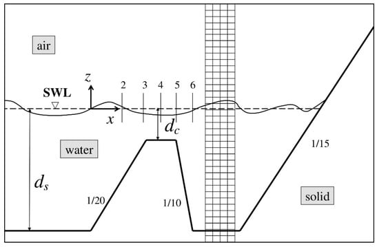
Figure 1.
Sketch of the computational domain and part of the Cartesian grid, as well as definitions of parameters for the numerical simulation of wave propagation over a submerged impermeable trapezoidal bar [27]. Note that the axes are not to scale. The distance from the wavemaker to the seaward toe of the bar is 27 dS, while the distance from the leeward toe of the bar to the toe of the absorbing beach is 5 dS.
The time step was selected so that the stability/convergence criteria of the numerical solution to be satisfied. These criteria are the CFL (Courant-Friedrichs-Lewy) and the VSL (Viscous Stability Limit). In the present work, the CFL and VSL limits were equal to 2 × 10⁻² and 7 × 10⁻⁴, respectively:
In order for the flow field not to be affected by the height of the air layer in the computational domain, this was selected to be 1.5dS above the SWL (after trial and error). The trapezoidal bar was impermeable; therefore, the no-slip condition on its surface was imposed using the IB method. Simulations were performed in the Greek supercomputer ARIS, deployed and operated by GRNET (Greek Research and Technology Network). ARIS consists of 532 computational nodes separated by four ‘islands’. We deployed only one of the ‘islands’: the thin nodes, which consist of 426 nodes and 8520 CPU cores. In this case, the simulation time was 1 wave period per 6 h on ARIS. Comparisons of the free-surface elevation between the numerical results and the experimental data in [27] at five locations (Figure 1) over the bar during the last five wave periods are presented in Figure 2. A good agreement is observed; the r.m.s. (root mean square) relative error between the numerical results and the experimental data at each location is reported in the caption of Figure 2.
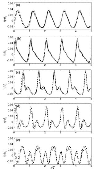
Figure 2.
Variation of the free-surface elevation during five wave periods, after 20 wave periods of simulation, at five locations over a submerged impermeable trapezoidal bar. These five locations correspond, respectively, to the stations 2, 3, 4, 5, and 6 of Figure 1. The lines correspond to the present numerical results while the symbols to the experiments in [27]. The r.m.s. (root mean square) relative error of the free-surface elevation between numerical results and experimental data is: (a) 0.09, (b) 0.13, (c) 0.16, (d) 0.19, and (e) 0.18.
The second validation case (Figure 3) corresponds to wave transmission over the wide-crested submerged permeable breakwater in [13]. In these experiments, waves of height H = 0.07 m and period T = 1.6 s were generated over a region of constant water depth dF = 0.4 m, which is followed by a beach of slope tanβ = 1/20 seawards of the breakwater. The depth at the breakwater toe was dS = 0.3 m, while the crest depth was dC = 0.05 m. As mentioned in the Introduction for these experiments, the trunk of the rubble-mound breakwater was permeable with a two-layer armor (D50 = 4.8 cm and n = 0.53) and a core with smaller rocks (D50 = 1.47 cm and n = 0.49). For the simulations (Figure 3), to achieve both adequate resolution in the wall boundary layer and a reasonable computational cost, the experiment was reproduced with dS = 0.12 m using Froude scaling, leading to a Reynolds number Red = 130,000, i.e., six times smaller than the one in the experiments. A mesh independence study was also performed. In order for the mesh not to affect the solution, the computational grid was selected to have a uniform size of Δx/dF = 0.02 along x (355 grid points per wavelength of the incident wave), and a non-uniform size in z; Δz/dF = 0.005 in the water and increasing to Δz/dF = 0.01 in the air. The corresponding values in the water with respect to the Stokes length, δ, were Δx/δ = 4.2 and Δz/δ = 1.06, which were sufficient to get a good resolution with at least five grid points in the wave boundary layer over the bed. The CFL and VSL criteria were equal to 2 × 10⁻² and 7 × 10⁻⁴, respectively. In order for the flow field not to be affected by the height of the air layer in the computational domain, this was selected to be 1.5dS above the SWL (after trial and error). The calibration values αp = 1000 and βp = 1.1, according to [19,20], were used in Equation (7); the values βp = 0.8 in the armor layer and βp = 1.2 in the core were also used, according to [13], but with negligible differences in the results.
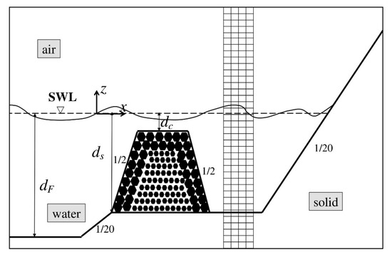
Figure 3.
Sketch of the computational domain and part of the Cartesian grid, as well as definitions of the parameters for the numerical simulation of wave propagation over submerged permeable breakwater [13]. Note that the axes are not to scale. The distance from the wavemaker to the toe of the 1/20 slope is 19.3dF, while the distance from the leeward toe of the breakwater to the toe of the absorbing beach is 4.5dF.
Snapshots of the free surface elevation during the two wave periods, after 20 wave periods of simulation (one wave period per 6 h on ARIS), are shown in Figure 4, in comparison to the experimental data of crest and trough elevations in [13]. The horizontal coordinate and the free surface elevation are shown dimensionless based on dF. The numerical model captures adequately the main characteristics of wave propagation over the submerged breakwater. More specifically, in the seaward region of the structure, the generation of a partially standing wave due to wave reflection is captured precisely by the model. In the vicinity of the crest and near the leeward region of the structure, the model captures adequately the wave dissipation due to wave breaking over the crest and due to filtration through the permeable trunk, while the wave height is under-predicted in the far leeward region. This last behavior is similar to the one observed in [16]. The maximum r.m.s. relative error of the wave height between the numerical results and the experimental data is reported in the caption of Figure 4.
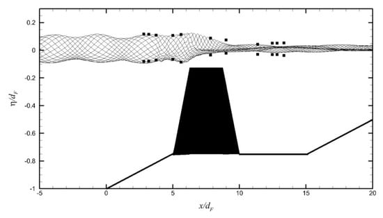
Figure 4.
Envelope of the free-surface elevation of waves passing over submerged permeable breakwater. The lines correspond to the present numerical results while the symbols to the experiments in [13]. The maximum r.m.s. relative error of the wave height between numerical results and experimental data is less than 0.05 in the seaward region and 0.32 in the far leeward region.
3. Results
All ZFBs in the present study were rubble mound and permeable with tana = 1/2 for both seaward and leeward slopes. A sketch of the computational domain is shown in Figure 5. First, three different setups were considered to examine the effect of crest width (cases 1–3 in Table 1) on the hydrodynamic processes of wave reflection, overtopping, transmission, and setup, as well as the flow behavior in the seaward and leeward regions of these structures. In cases 1–3, the ZFBs were fully-permeable (homogeneous trunk permeability), while the crest width, B, was set equal to dS, 2dS, and 3dS, respectively, where dS is the constant water depth between the wavemaker and the seaward ZFB toe. Then, the effect of the incident wave period (cases 1 and 4 in Table 1) and the ZFB trunk permeability (cases 1 and 5 in Table 1) were also investigated for the ZFB case with B = dS.
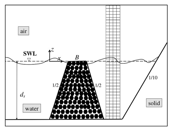
Figure 5.
Sketch of the computational domain and part of the Cartesian grid for the permeable ZFB cases. Note that the axes are not to scale. The distance from the wavemaker to the seaward ZFB toe is 23dS, while the distance from the leeward ZFB toe to the toe of the absorbing beach is 9dS.

Table 1.
Geometrical characteristics of the examined ZFB cases, the parameters of the incoming waves and the breaking ones on the seaward slope of the ZFB.
In dimensional terms, dS was selected to be equal to 0.4 m, which corresponds to Reynolds number Red = 800,000. The geometrical details and the incident wave parameters for all cases are summarized in Table 1. For all cases, a grid independence study was performed, and the selected computational grid had a uniform size of Δx/dS = 0.02 along x (300–450 grid points per wavelength of the incident waves), and a non-uniform size in z; Δz/dS = 0.0025 in the water and increasing to Δz/dS = 0.01 in the air. The corresponding values in the water with respect to the Stokes length, δ, were Δx/δ = 10.1 ÷ 12.1 and Δz/δ = 1.27 ÷ 1.51 according to the wave length, which were sufficient to get a good resolution with at least four grid points in the wave boundary layer over the bed. The small flow scales occurring during breaking at the ZFB seaward slope are modeled by the SGS eddy-viscosity model. In all simulations, the CFL and VSL criteria were equal to 2.0 × 10⁻² and 5 × 10⁻⁴, respectively. In order for the flow field not to be affected by the height of the air layer in the computational domain, this was selected to be 1.5dS above the SWL (after trial and error). The calibration values αp = 1000 and βp = 1.1, according to [19,20], were used in Equation (7).
Typical crest and trough elevation envelopes during 10 wave periods, after 20 wave periods of simulation (1 wave period per 6 h on ARIS), are shown in Figure 6 for case 1. From such envelope results, the breaking depth on the seaward ZFB slope and the corresponding wave height were identified at the location of the maximum wave crest elevation. In all cases, wave breaking occurred on the seaward slope and near the crest of the ZFBs; these results are summarized in Table 1. In cases 1–3, which correspond to the same incident wave and different crest width, the waveform in the seaward region of the ZFBs is similar, and a partially standing wave is generated due to reflection. In the leeward region of the ZFBs, the wave height, i.e., the wave energy, is different between cases 1–3 as it decreases with the increase of the crest width. In case 4, a decreased wave height is observed in the seaward region, while less wave energy is transmitted to the leeward region in comparison to case 1, which has the same crest width but larger incident wave period, i.e., a longer incident wavelength. In case 5, where the ZFB has a less permeable core, a slightly increased wave height is observed in the seaward region and slightly less wave energy is transmitted to the leeward region in comparison to case 1, which has the same crest width but larger ZFB trunk permeability.
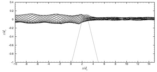
Figure 6.
The envelope of the free surface elevation of waves breaking over the ZFB case 1.
The behavior of wave height in the seaward and leeward side of all ZFB cases is also demonstrated in terms of the reflection and transmission coefficients presented in Table 2. For the reflection coefficient, surface elevation time series at three locations in the seaward region of the ZFBs were obtained, and a reflection analysis was performed using the method in [28]. For the transmission coefficient, the surface elevation time series, recorded at the seaward and leeward toe of the ZFBs, were used to calculate the wave height at each position through spectral analysis. It is observed that wave transmission decreased, while wave reflection did not vary, with the increase of the crest width (cases 1–3) when incident wave height, incident wave period, and trunk permeability did not change. The decrease of wave transmission is attributed to the increase of wave dissipation over the ZFB crest as B increased. Decreasing the incident wave period (cases 1 and 4) results in the decrease of wave reflection and the decrease of wave transmission when the crest width and trunk permeability did not change. These decreases are associated with the decrease of ξ0. Finally, reducing trunk permeability (cases 1 and 5) also increased the wave reflection and decreased the wave transmission when crest width and incident waves did not change. Wave energy transmission was affected by both the overtopping over the ZFB crest and the porous flow in the ZFB trunk. In case 5, the less permeable ZFB trunk inhibited the transmission of kinetic energy through the trunk from the seaward to the leeward region of the ZFB in comparison to case 1, thus, the resulting reflection coefficient, Kr, was larger and the transmission coefficient, Kt, was smaller.
Table 2.
Reflection and transmission coefficients for all the ZFB cases of Table 1.
Apart from the computed reflection and transmission coefficients, the corresponding values predicted by widely used empirical formulas are also presented in Table 2. For wave reflection, the empirical formula of Equation (1) was used, with γf = 0.40, for the fully-permeable ZFB cases 1–4, and γf = 0.5, for the partially-permeable ZFB case 5, according to [1]. To achieve the best possible agreement to the computed results, the reduction parameter was set to C = 0.43 instead of the value C = 0.67 suggested in [1] for ZFBs. For wave transmission, the empirical formulas of Equation (3) were used. Overall, better prediction seems to be achieved by the empirical formula in [5].
The distribution of the instantaneous vorticity field in the vicinity of the ZFB case 1, at four instants during the 30th wave period of the simulation, is presented in Figure 7. It is shown that as the wave trough reached the breakwater crest (down-rush flow phase), strong anti-clockwise vorticity developed near above the seaward slope of the structure. As the wave propagated and the flow reversed (up-rush flow phase), this vorticity layer was separated from the slope and vortices were generated and transported offshore, while a new vorticity layer of opposite sign (clockwise) formed near above the slope. During the down-rush flow phase, there was no separation of this vorticity layer. In cases 2 and 3, there were no notable differences in the vorticity behavior above the seaward slope of the ZFBs. In case 4, with a shorter wavelength in comparison to case 1, the vorticity behavior was similar, but the offshore transportation of the vortices was extended to a shorter distance (Figure 8). In case 5, with a less permeable ZFB trunk in comparison to case 1, the vorticity behavior near the crest was similar, while a weak vorticity layer was generated at the interface between the armor layer and the core in the ZFB trunk (Figure 9).
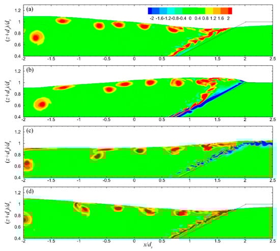
Figure 7.
Vorticity field in the seaward region of ZFB case 1 at four instants during the 30th wave period: (a) T/3, (b) 3T/8, (c) 5T/8, and (d) T.
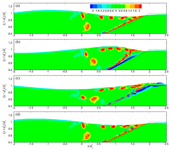
Figure 8.
Vorticity field in the seaward region of the ZFB case 4 at four instants during the 30th wave period: (a) T/3, (b) 3T/8, (c) 5T/8, and (d) T.
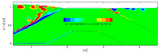
Figure 9.
Vorticity field near the crest and in the ZFB trunk (case 5) at one instant (T/8) during the 30th wave period.
The period-mean velocity field (of 10 wave periods after 20 wave periods of simulation) in the seaward region of the ZFBs in cases 1–3 is presented in Figure 10. It is highlighted that in these cases, the generated currents above the ZFB seaward slope and crest were directed onshore due to wave overtopping, while the currents in the ZFB trunk were weaker and directed offshore. In the leeward region of these ZFBs, the period-mean velocity field is presented in Figure 11. It is shown that as the crest width increased, the magnitude of the velocities became weaker. The period-mean velocity in the seaward and leeward regions of the ZFB case 4 is presented in Figure 12. The direction of the currents in the seaward and leeward regions of the ZFB follows the same pattern as in case 1, but their magnitude was smaller in both regions due to the lower energy transmission onshore. The period-mean velocity field for the ZFB case 5 is presented in Figure 13. The magnitude of the currents in the seaward and leeward regions and the ZFB trunk was slightly larger in comparison to case 1.
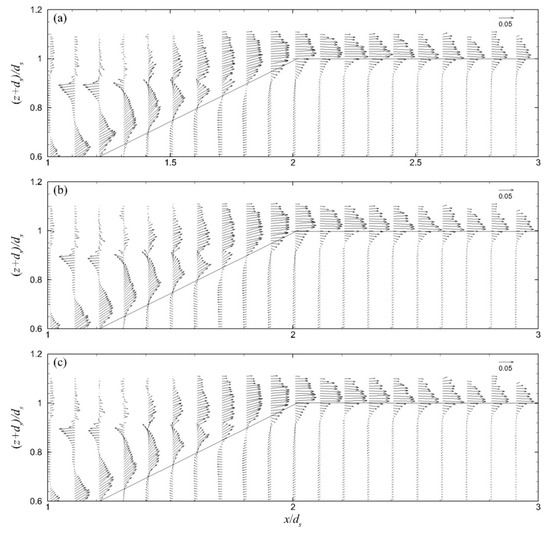
Figure 10.
Period-mean velocity field in the seaward region of the ZFBs in cases: (a) 1, (b) 2, and (c) 3. Velocity vectors are shown non-dimensionalized by (gdS)1/2 in the water phase under the wave crest envelope.
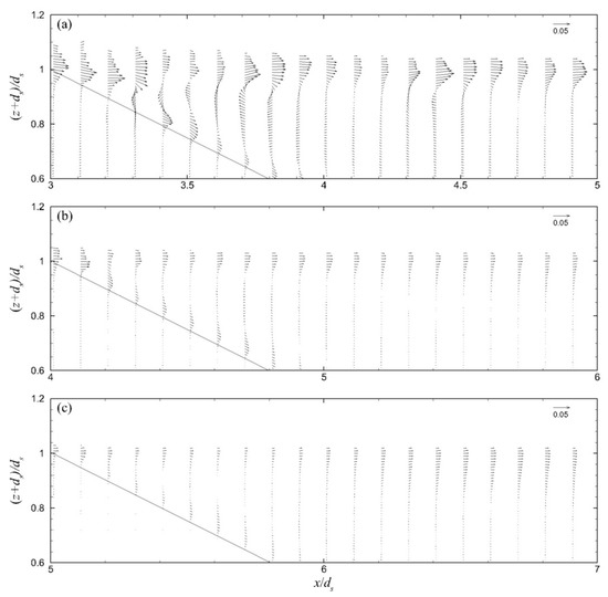
Figure 11.
Period-mean velocity field in the leeward region of the ZFBs in cases: (a) 1, (b) 2, and (c) 3. Velocity vectors are shown non-dimensionalized by (gdS)1/2 in the water phase under the wave crest envelope.
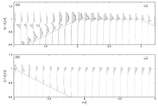
Figure 12.
Period-mean velocity field for ZFB case 4 in: (a) the seaward region, and (b) the leeward region. Velocity vectors are shown non-dimensionalized by (gdS)1/2 in the water phase under the wave crest envelope.
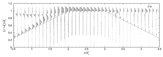
Figure 13.
Period-mean velocity field for ZFB case 5. Velocity vectors are shown non-dimensionalized by (gdS)1/2 in the water phase under the wave crest envelope.
The period-mean flow pattern in the vicinity of the ZFBs for cases 1–3 is illustrated through streamlines in Figure 14. It is demonstrated that in the ZFB trunk, the flow was directed offshore in all cases. Part of the flow that overtops the crest of the ZFBs returned offshore through the ZFB trunk; as a result, the water renewal was facilitated in the ZFB leeward region. This process is obvious in cases 1 and 2. Further increase of the crest width though (case 3) results in the limitation of the flow circulation cell in the ZFB trunk and the interruption of water renewal in the ZFB leeward region through the ZFB trunk. The pattern of the streamlines in ZFB case 4 does not differ from the one in case 1, and it is not shown. For the ZFB case 5 (Figure 15), the return flow from the leeward to the seaward region through the ZFB trunk is inhibited by the presence of a less permeable core than in case 1.
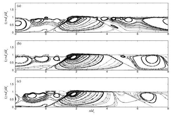
Figure 14.
Streamlines in the vicinity of the ZFBs in cases: (a) 1, (b) 2, and (c) 3.
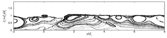
Figure 15.
Streamlines in the vicinity of ZFB case 5.
The mean overtopping discharge, q, over and through the ZFBs, and the wave setup, δ, in the leeward region of the ZFBs are shown in Table 3. The overtopping discharge was computed as the period-mean (of 10 wave periods after 20 wave periods of simulation) flux through the vertical cross-section at the leeward end of the ZFB crest. The instantaneous flux is:
where dlc(t) is the instantaneous water level at the leeward end of the ZFB crest. The mean overtopping discharge comprises the discharge through the ZFB trunk and the crest discharge over the ZFB crest. The corresponding results are also shown in Table 3. The wave setup, δ, was computed as the period-mean (of 10 wave periods after 20 wave periods of simulation) free-surface level over the SWL at the leeward ZFB toe.
Table 3.
Mean overtopping discharge and wave setup for all the ZFB cases (Table 1).
For ZFB case 1, the trunk discharge is in the offshore direction (negative), while the one over the crest is in the onshore direction (positive). As B increased, for ZFB cases 2 and 3, the negative trunk discharge weakened and even turned positive in case 3, while the one over the crest weakened as well but remained positive. The overall mean overtopping discharge was always onshore and it decreased, albeit weakly, with the increase of the ZFB crest width. The decrease of ξ0 in ZFB case 4, in comparison to case 1, also resulted in the weak decrease of the mean overtopping discharge. In ZFB case 5, both the trunk discharge and the one over the crest strengthened in comparison to the ones in case 1, but the mean overtopping discharge decreased. To apply Equation (4) in the present cases, which were laboratory-scale ones since dS = 0.4 m, an adjustment factor of fq = 8.2 was used, which is lower than the maximum value of 11 suggested in EurOtop [6] for tana = 1/2. The mean overtopping discharge predicted by Equation (4) was constant for all ZFB cases, as shown in Table 3, reflecting the strong dependence of q on Hi but not the one on B, ξ0, and permeability as the present results suggest.
The wave setup increases with increasing B, for ZFB cases 1 and 2, but it decreases again for ZFB case 3 despite the further increase of B because of the interruption of the flow circulation cell in the ZFB trunk for case 3 as shown in Figure 14c. The decrease of ξ0 in ZFB case 4, in comparison to case 1, resulted in the decrease of the wave setup, while the decrease of permeability in ZFB case 5 increased the wave setup. The corresponding wave setup predicted by the empirical formulas of Equation (5) overestimated δ (Table 3) since they were both based on experiments without the recirculation system described in the Wave Generation subsection.
Finally, the instantaneous shear stress field for ZFB case 5 at two instants during the 30th wave period of the simulation is presented in Figure 16. During the up-rush flow phase and as the wave crest approaches the breakwater crest, significant positive shear stress was observed near the seaward slope of the structure, while a positive layer was also developed in between the two different materials inside the porous media. Shear stress of opposite sign was developed in the same areas during the down rush flow phase. As expected, the seaward slope of the ZFB was the most crucial part of the structure in terms of hydraulic stability, as it experienced larger values of the developing shear stress, i.e., the destabilizing force due to wave breaking.
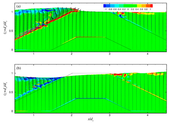
Figure 16.
Shear stress for case 5 at two instants during the 30th wave period: (a) T/2, and (b) T.
4. Discussion
In the present work, the effect of ZFB crest width, breaking parameter, and ZFB trunk permeability on wave reflection, crest overtopping, wave transmission, wave setup, and wave-generated currents were studied numerically.
The results indicate that the size of the crest width, B, did not notably affect wave (reflection coefficient) and flow (instantaneous vorticity and period-mean currents) processes in the seaward region of ZFBs. However, the processes in the leeward region of ZFBs were significantly affected by B; wave transmission and magnitude of currents decreased with increasing B. In addition, the mean overtopping discharge heading onshore decreased, albeit weakly, with increasing B. The effect of B on the wave setup was not monotonic as it depended on the pattern of the flow circulation in the ZFB trunk, but eventually this also decreased with increasing B. The effect of the breaking parameter, ξ0, and the ZFB trunk permeability on wave and flow processes were significant both in the seaward and leeward regions of ZFBs. As ξ0 decreased, the wave reflection, wave transmission, magnitude of currents, mean overtopping discharge, and wave setup all decreased; this observation is in accordance with the relevant empirical formulas (Table 2 and Table 3) considered in this study. Finally, decreasing the ZFB trunk permeability led to the increase of wave reflection, the magnitude of currents, and wave setup, but to the decrease of wave transmission and mean overtopping discharge.
Therefore, for the design of ZFBs, decreasing trunk permeability is equivalent to increasing crest width in terms of the wave and hydrodynamic processes in the leeward region of ZFBs as far as wave transmission and mean overtopping discharge are concerned, but not equivalent for wave setup and magnitude of currents. If the latter parameters are not critical, decreasing the ZFB trunk permeability is a more economical option compared to the increase of crest width.
Author Contributions
Conceptualization, T.I.K. and A.A.D.; methodology, T.I.K. and A.A.D.; software, T.I.K.; validation, T.I.K.; formal analysis, T.I.K. and A.A.D.; investigation, T.I.K.; resources, A.A.D.; data curation, T.I.K.; writing—original draft preparation, T.I.K.; writing—review and editing, A.A.D.; visualization, T.I.K.; supervision, A.A.D.; project administration, A.A.D.; funding acquisition, A.A.D. All authors have read and agreed to the published version of the manuscript.
Funding
This paper is part of the research project ARISTEIA I - 1718, implemented within the framework of the Education and Lifelong Learning program, and co-financed by the European Union (European Social Fund) and Hellenic Republic funds.
Acknowledgments
This work was supported by the computational time granted by the Greek Research & Technology Network (GRNET) in the National HPC facility ARIS under project ID CoastHPC.
Conflicts of Interest
The authors declare no conflict of interest. The funders had no role in the design of the study; in the collection, analyses, or interpretation of data; in the writing of the manuscript, or in the decision to publish the results.
References
- Zanuttigh, B.; van der Meer, J.W. Wave reflection from coastal structures in design conditions. Coast. Eng. 2008, 55, 771–779. [Google Scholar] [CrossRef]
- Seelig, W.N. Two-Dimensional Tests of Wave Transmission and Reflection Characteristics of Laboratory Breakwaters. Coast. Eng. Res. Cent. 1980. [Google Scholar] [CrossRef]
- Seabrook, S.R.; Hall, K.R. Wave transmission at submerged rubble mound breakwaters. In Proceedings of the 26th International Conference on Coastal Engineering, Copenhagen, Denmark, 22–26 June 1998. [Google Scholar] [CrossRef]
- Van der Meer, J.W.; Briganti, R.; Zannuttigh, B.; Wang, B. Wave transmission and reflection at low-crested structures: Design formulae, oblique wave attack and spectral change. Coast. Eng. 2005, 52, 915–929. [Google Scholar] [CrossRef]
- Buccino, M.; Calabrese, M. Conceptual Approach for Prediction of Wave Transmission at Low-Crested Breakwaters. J. Waterw. Port Coast. Ocean Eng. 2007, 133, 213–224. [Google Scholar] [CrossRef]
- Van der Meer, J.W.; Allsop, N.W.H.; Bruce, T.; De Rouck, J.; Kortenhaus, A.; Pullen, T.; Schüttrumpf, H.; Troch, P.; Zanuttigh, B. EurOtop, Manual on Wave Overtopping of Sea Defences and Related Structures. An. Overtopping Manual Largely Based on European Research, but for Worldwide Application; Envrionment Agency, ENW, KFK: Bristol, UK, 2018. [Google Scholar]
- Diskin, M.H.; Vajda, M.L.; Amir, I. Piling-up behind low and submerged permeable breakwaters. J. Waterw. Harb. Coast. Eng. Div. 1970, 96, 359–372. [Google Scholar] [CrossRef]
- Loveless, J.H.; Debski, D.; McLeod, A.B. Sea level set-up behind detached breakwaters. In Proceedings of the 26th International Conference on Coastal Engineering, Copenhagen, Denmark, 22–26 June 1998; pp. 1665–1678. [Google Scholar] [CrossRef]
- Bellotti, G. A simplified model of rip currents systems around discontinuous submerged barriers. Coast. Eng. 2004, 51, 323–335. [Google Scholar] [CrossRef]
- Calabrese, M.; Vicinanza, D.; Buccino, M. 2D Wave setup behind submerged breakwaters. Ocean Eng. 2008, 35, 1015–1028. [Google Scholar] [CrossRef]
- Mitzutani, N.; Mostafa, A.M.; Iwata, K. Nonlinear regular wave, submerged breakwater and seabed dynamic interaction. Coast. Eng. 1998, 33, 177–202. [Google Scholar] [CrossRef]
- Huang, C.J.; Chang, H.H.; Hwung, H.H. Structural permeability effects on the interaction of a solitary wave and a submerged breakwater. Coast. Eng. 2003, 49, 1–24. [Google Scholar] [CrossRef]
- Garcia, N.; Lara, J.L.; Losada, I.J. 2-D numerical analysis of near-field flow at low-crested permeable breakwaters. Coast. Eng. 2004, 51, 991–1020. [Google Scholar] [CrossRef]
- Hsu, T.J.; Sakakiyama, T.; Liu, P.L.F. A numerical model for wave motions and turbulence flows in front of a composite breakwater. Coast. Eng. 2002, 46, 25–50. [Google Scholar] [CrossRef]
- Losada, I.J.; Lara, J.L.; Christensen, E.D.; Garcia, N. Modelling of velocity and turbulence fields around and within low-crested rubble-mound breakwaters. Coast. Eng. 2005, 52, 887–913. [Google Scholar] [CrossRef]
- Lara, J.L.; Garcia, N.; Losada, I.J. RANS modelling applied to random wave interaction with submerged permeable structures. Coast. Eng. 2006, 53, 395–417. [Google Scholar] [CrossRef]
- Kramer, M.; Zanuttigh, B.; van der Meer, J.W.; Vidal, C.; Gironella, X. Laboratory experiments on low-crested breakwaters. Coast. Eng. 2005, 52, 867–885. [Google Scholar] [CrossRef]
- Dimas, A.A.; Koutrouveli, I.T. Wave Height Dissipation and Undertow of Spilling Breakers over Beach of Varying Slope. J. Waterw. Port Coast. Ocean Eng. 2019, 145. [Google Scholar] [CrossRef]
- Liu, P.L.F.; Pengzhi, L.; Chang, K.; Sakakiyama, T. Numerical modeling of wave interaction with porous structures. J. Waterw. Port Coast. Ocean Eng. 1999, 125, 322–330. [Google Scholar] [CrossRef]
- Van Gent, M.R.A. Wave Interaction with Permeable Coastal Structures. Ph.D. Thesis, Delft University, Delft, The Netherlands, 1995. [Google Scholar]
- Keulegan, G.H.; Carpenter, L.H. Forces on cylinders and plates in an oscillating fluid. J. Res. Nat. Bur. Stand. 1958, 60, 423–440. [Google Scholar] [CrossRef]
- Smagorinsky, J. General circulation experiments with the primitive equations: I. The basic experiment. Mon. Weather Rev. 1963, 91, 99–164. [Google Scholar] [CrossRef]
- Yang, J.; Stern, F. Sharp interface immersed-boundary/level-set method for wave–body interactions. J. Comput. Phys. 2009, 228, 6590–6616. [Google Scholar] [CrossRef]
- Balaras, E. Modeling complex boundaries using an external force field on fixed Cartesian grids in large-eddy simulations. Comput. Fluids 2004, 33, 375–404. [Google Scholar] [CrossRef]
- Hughes, S.A. Physical Models and Laboratory Techniques in Coastal Engineering; World Scientific: Singapore, 1993; pp. 367–379. [Google Scholar] [CrossRef]
- Jacobsen, N.G.; Fuhrman, D.R.; Fredsoe, J. A wave generation toolbox for the open-source CFD library: Open Foam®. Int. J. Numer. Methods Fluids 2011, 70, 1073–1088. [Google Scholar] [CrossRef]
- Beji, S.; Battjes, J.A. Numerical simulation of nonlinear wave propagation over a bar. Coast. Eng. 1994, 23, 1–16. [Google Scholar] [CrossRef]
- Mansard, E.P.D.; Funke, E.R. The measurement of incident and reflected spectra using a least squares method. In Proceedings of the 17th International Conference on Coastal Engineering, Sydney, Australia, 23–28 March 1980; pp. 154–172. [Google Scholar] [CrossRef]
© 2020 by the authors. Licensee MDPI, Basel, Switzerland. This article is an open access article distributed under the terms and conditions of the Creative Commons Attribution (CC BY) license (http://creativecommons.org/licenses/by/4.0/).