Abstract
In the present study, the overall stability of typical Korean composite caisson breakwaters that were initially designed following the conventional deterministic approach is investigated using reliability approaches. Therefore, the sensitivity of critical uncertainties regarding breakwater safety is analyzed. Uncertainty sources related to the structure, ocean conditions, and properties of the subsoil and rubble mound are considered in the reliability analysis. Sliding and overturning failures are presented as explicit equations, and three reliability methods, i.e., the mean value first-order second-moment, first-order reliability method, and Monte Carlo simulation, are applied in the evaluation process. Furthermore, the bearing capacity of the rubble mound and subsoil are analyzed using the discrete slice method conjugated with the Monte Carlo simulation. The results of this study establish that the sliding failure generally is the most frequent failure occurring among the above-mentioned overall stability failures (around 15 times more common than failures observed in the foundation). Additionally, it is found that the horizontal wave force primarily contributes to the sliding of the caisson body, whereas the friction coefficient is the main factor producing the resistance force. Furthermore, a much small probability of overturning failure implies that the overturning of a caisson around its heels uncommonly occurs during their lifetime, unlike other overall failure modes. Moreover, the failure in foundations may commonly encounter in the breakwater that has a high rubble mound structure compared with sliding mode. Particularly, the performance function of the all foundation bearing capacities presents a nonlinear behavior and positively skewed distribution when using the Monte Carlo simulation method. This phenomenon proves that simulation methods might be an appropriate approach to evaluate the bearing capacity of a breakwater foundation that can overcome several drawbacks of the conventional design approach.
1. Introduction
A breakwater (BRW) is a vital structure that is used to mitigate effects of ocean random seas such as storm surges with extreme wave and tide variations, to provide a calm basin for protecting port facilities and mooring ships. BRWs play a critical role in the port operation, especially for ports located in the rough seas [1]. A composite BRW type generally consists of a precast concrete caisson filled with material and a rubble mound arranged above the seabed. The armor units can be made by the precast concrete block, such as Dolos or Tetrapod, that is placed beside the caisson structure to absorb most of the incident wave energy. Vertical composite BRWs are widely used in deep-water sites because they are more cost-efficient compared with rubble mound types [2,3].
Vertical composite BRWs, which have a lot of advantages, were firstly applied in 1910 at Kobe Port. Thereafter, several catastrophic failures occurred, such as Bizerta (Tunisia) in 1915, Niigata West Port (Japan) in 1930, and Mustapha (Algiers) in 1934 [2,4]. Consequently, the vertical BRW was mostly abandoned in favor of the rubble mound type. However, at the end of the 1970s and in the early 1980s, the rubble mound BRW also experienced a series of failures. The severe damages was a catalyst for a different approach in the design of BRWs, namely the probabilistic method [3,5].
In the conventional design approach (CDA), the structures are classified as acceptable or unacceptable by comparing the nominal safety factors with those specified in the design standard. For instance, the safety factors against the sliding and overturning should not be lower than 1.2, as required in [6,7]. In general, the more important the structures, the higher the safety factors (FS) that should be selected. Thereby, the safety level of the structures can be increased. However, an increase in the specified FS without considering the inherent uncertainty of variables might not accurately reflect the overall contribution of the different input variables. In other words, the effects of all input variables may not contribute equally to the FS estimation. This assumption may cause a significant increase in the construction cost, whereas a sufficient safety level might not be obtained as expected.
In addition, the CDA might not account for most of the failure modes of BRWs, as stated by Oumeraci [5] in 1993. The author concluded that the dynamics analysis and probabilistic design approaches seem to be the only feasible solutions to solve the integrated stability problem of vertical BRWs. Moreover, additional statistical information needs to be provided before applying a reliability analysis, which is not necessary for the CDA. However, the valuable information from the reliability results makes it possible to provide more reasonable decisions in the design process compared with those obtained from the CDA [8]. The stability of armor layers was first studied by applying probabilistic approach in the work of Van der Meer [9]. Based on the probabilistic studies, systems of partial safety factor were developed for rubble mound BRWs by the Permanent International Association of Navigation Congresses (PIANC) Permanent Technical Committee II (PTC II ) Working Group 12 [10,11] and for vertical BRW types by the PIANC PTC II Working Group 28 [12,13].
In Korea, BRW structures are primarily designed using the traditional deterministic method [6,14]. Recently, some failure modes based on reliability have been studied. Most of these studies deal with the stability of the armor layer or rubble mound BRWs [14,15]. Although the stability of vertical BRWs has also been studied, not as much attention has been paid to the overall failure modes compared with that for the sliding mode of the caisson on a rubble mound, as presented in previous researches [14,16,17]. However, BRWs are commonly located in enormous energy potential zones of ocean waves, so they intrinsically face various probable failure aspects. Possible ruptures, including overall and local failure modes, have been presented in previous studies [5,10,11,18,19]. Theoretically, all possible failure aspects need to be investigated before making any final design decisions. Furthermore, in Japan, the overall failure modes of BRWs, i.e., the caisson sliding [16,18,19] and foundation failure [4,10,13,20] have been reported as the most common failures observed. Therefore, the three most frequent overall failure modes, the caisson sliding on the rubble mound surface, insufficient foundation bearing capacity, and the overturning of a caisson around its heel, are examined in this study, as shown in Figure 1a–c. The parts labeled 1 and 2 are the caisson and rubble mound structures, respectively.

Figure 1.
Overall failure mode of breakwaters (BRWs) studied: (a) Sliding, (b) Insufficient foundation bearing capacity, (c) Overturning.
In Europe, Level 1 and Level 2 probabilistic analyses have been developed, while Level 3 has been successfully carried out in Japan [19]. Notably, the Level 1 and Level 2 reliability design methods are based on the mean value first-order second-moment (MVFOSM), and first-order reliability method (FORM), respectively [11,12], whereas the Level 3 reliability design method is related to the estimation of the caisson sliding distance [18,19,21,22] or the expectation of damages occurring in the armor blocks of horizontal composite BRWs [23]. In this study, the safety of nine typical Korean vertical BRWs is estimated using different reliability analysis methods, MVFOSM, FORM, and the Monte Carlo Simulation (MCS). Hence, this study would provide a reliability-based comprehensive assessment of the overall stability of BRWs that were initially designed using the CDA.
Furthermore, three primary uncertainty sources [i.e., properties inherent to the structure itself (uncertainties in the density of materials), the hydraulic climate (randomness of tide level and wave force), and soil properties of the foundation] are also explored in this study. Thereafter, a sensitivity analysis is performed to find the most critical uncertainties that predominantly contribute to structural damage.
In order to obtain the above-mentioned purposes, several functions are developed in MATLAB to carry out the reliability-based analysis. By doing so, valuable insight into the overall BRW stability is provided. The rest of the study is presented as follows: Section 2 summarizes the reliability approaches used in the study. Section 3 focuses on the sliding and overturning failure modes of the caisson structure. Section 4 investigates the bearing capacity of the foundation by circular slip failure analysis using Bishop’s simplified method (BSM) conjugated with MCS. Finally, Section 5 concludes the study.
2. Selection of Reliability Approaches
A reliability index (RI) called the Cornell reliability (CR) index was first estimated in 1969 by Cornell. The CR index is determined as the ratio of the first and second moments of the performance function (PF) at the mean value of all input variables [24]. However, accurate results can be obtained using this method only when the PF is linear and the variances of input variables are not too large [25]. In 1974, Hasofer and Lind [26] proposed another index called the Hasofer-–Lind (HL) index, which overcomes the drawbacks of the CR index owing to the assumption on the distributions of the involved variables in the analysis [27]. The HL index is defined as the shortest distance from the origin to the PF surface plotted in the standard normalized space. Therefore, the estimation of the HL index becomes an optimization problem in the standard normalized space. In this problem, if the input variables have non-normal distributions, Rosenblatt’s transformation is commonly applied to convert the variables from their space to the standard normalized space [25,27]. The most probable point (MPP) or the design point is the point that satisfies both constraint conditions, i.e., (1) belongs to the performance surface and (2) causes the shortest distance to the origin. The PF is estimated at the MPP as an equivalent linear function and nonlinear function corresponding to the FORM and the second-order equation (SORM) using Taylor’s expansion.
The purpose of the Monte Carlo Simulation (MCS) is to simulate the PF on the space of the initial input variables, generally consisting of two steps. Firstly, all involved variables associated with their cumulative distribution are randomly generated. Secondly, the occurrence of failure states is evaluated by comparing the estimated PF value in each sampling with a certain boundary condition. The probability of failure is then determined as the proportion of the total number of failures in the simulation [25,27].
Among the above-mentioned reliability methods, the best accuracy results can be achieved most frequently with the MCS, but it requires the most time for analysis. The MCS is the reasonable choice for large-dimension problems or when the PFs are nonlinear or implicitly defined, e.g., estimation of the bearing capacity of foundations by BSM. However, problems with low failure probabilities would require an extremely large simulation to recognize a sufficient number of failures. In these cases, the crude MCS process is too time-consuming. Hence, some variance reduction techniques should be applied as better options in the simulation [25,27].
The estimation of the CR index is the simplest method, in which the worst-case outcome is the result of the most severe combination of all involved variables (the mean values). Based on Taylor’s expansion, the PF is approximated at the worst point of all the variables. However, Cornell’s estimation is a conservative method in most cases because the simultaneous occurrences of all input variables while also contributing to the outcome are only an idealization. Moreover, the information on the distribution type of random variables is ignored, and the CR index might not capable when the random variables have a considerable variation.
The FORM is widely used in practice [28,29]. However, it is difficult to evaluate the PF accurately in both FORM and SORM in highly nonlinear problems, especially problems with high dimensions. In general, more accurate results can be achieved by applying a combination of the MCS and FORM, thereby overcoming the disadvantage of individual methods. In this study, three methods, MVFOSM, FORM, and MCS are applied to assess sliding and overturning conditions of caissons since the PFs are explicitly defined, while the MCS is merely applied to evaluate the foundation bearing capacity, which is defined as a sophisticated and implicit PF.
3. Sliding and Overturning Failure Modes
3.1. Breakwater Structures and Wave Force Model
The present study analyzes the vertical BRWs and nine BRWs are intuitively chosen along the Korean shoreline, as shown in Figure 2. The typical section of caissons is shown in Figure 3, while their overall design conditions are listed in Table 1. In Table 1 and Figure 3, Bc and Hc represent the width and the heights of the caisson, respectively. hr indicates the height of the rubble mound. The ocean conditions are represented by the water depth at the site h, the water depth from the base of the caisson h′, the water depth over the berm d, and the variation in the tide level WL. Finally, the wave conditions are represented by the design wave height HD.
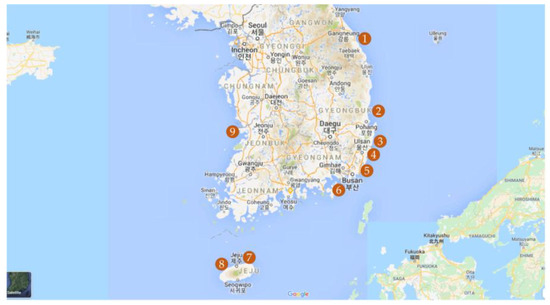
Figure 2.
Locations of breakwaters considered in this study.
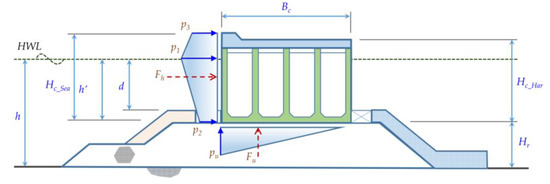
Figure 3.
Typical cross-section of a BRW and wave force model.

Table 1.
Dimensions and Environmental Characteristics of the breakwaters.
The wave forces (Fh and Fu) acting on the upright section are calculated using Goda’s formulae [30]. In Goda’s model, wave forces are determined from the pressures distributed over the height and width of the upright section, which are estimated based on the design wave height, determined by the mean of the 0.4% largest wave heights in the recorded wave data. The pressure is distributed triangularly on the bottom of the caisson (maximum pressure pu) and has a trapezoidal shape on the front face of the upright section (represented by pressure p1, p2, and p3). Figure 3 illustrates the wave pressures following Goda’s model on the caisson section.
3.2. Performance Functions and Considered Random Variables
In order to perform the reliability analysis, the PFs or limit state functions that consist of input variables need to be introduced. In the sliding case, the PF includes the driving force caused by the horizontal wave force and the resisting force related to the friction force between the bottom face of the caisson and the rubble mound surface. The friction force is a product of the effective normal force on the rubble mound and the friction coefficient. The PF for overturning conditions is similar to sliding but reflects the moments around the heels of the caisson. Namely, the mobilizing moment is generated by the wave forces and buoyancy force while the resisting moment is produced by the weight of the structure. Generally, sliding and overturning damages due to positive wave forces, i.e., from the seaside toward the harbor, are more critical than those from negative wave forces [19], which are also of interest in this study. The explicit performance equations, g(X) are shown in Equations (1) and (2) corresponding to sliding and overturning states.
where Lc, Lrc, and Lf are the lever arms of the moments caused by the weights of the plain concrete structure (Dc), the reinforced concrete structure (Drc), and the filling material (Df), respectively. The total weight of the materials comprising the caisson is represented as a summarized random input variable with a mean density of 2100 kg/m3 in [19]. In this work, these dead loads are considered as uncertainties with different variations, which are dependent on not only the construction stage but also the construction method. For instance, the caisson body is a precast reinforced concrete structure, so it would have better quality control compared with the concrete cover slab or filling material built on sites. The friction coefficient between the concrete caisson and the rubble surface, fc has been well studied and empirically obtained through various studies [13,18]. Here, its bias is presumed as a normal distribution with the mean value of 1.06 and coefficient of variation (COV) of 0.15. B stands for buoyancy force that is highly dependent on the submerged volume of the structure below the water level. Additionally, because tidal variations influence not only the buoyancy force but also wave pressures, the water level is studied as an uncertainty based on the tide fluctuations in this study. Tide levels rely on astronomical and meteorological tides and the increased water level caused by nearshore waves [28,29]. In the present study, different BRWs on the eastern, northern, or western coasts, as shown in Figure 2, are dissimilarly explored to consider the different variations in the tide levels.
Failures would occur whenever the mobilizing resultants exceed the resisting resultants. In principle, all parameters have themselves variation; however, some parameters with slight variations can be approximated as a deterministic approach with almost no effects on the final result [13]. Notably, because of the good quality managements, the dimensions of the caisson are assumed to be the same as the design, which means all lever arms in the overturning situation are treated in a deterministic manner in this study. The statistical information of the involved variables is summarized in the Table 2.

Table 2.
Statistical properties of the uncertainties applied in the overall stability analysis.
The vertical wave force, Fu, and horizontal wave force, Fh, estimated using Goda’s expression, are the random input variables in the study. It is proved that the wave forces obtained following the Goda’s formulae are conservative in the studies of Van der Meer et al. [13,31]. In other words, when Goda’s model is applied, the bias factor, λ, must be taken into account, which is generally less than unity [13], as shown in Equation (3).
Van der Meer et al. [31] compared Goda’s results with the model tests and proposed an overestimation of the Goda formulae. Vrijling [32] demonstrated through experiments that the derived standard deviation also included statistical uncertainty in the maximum wave height and the author suggested that the statistical information has a the lognormal distribution. Furthermore, Coastal Engineering Manual (CEM 2011) [28] in the United States proposed a somewhat different standard deviation relying on whether or not the model tests are performed. The statistical parameters related to wave forces are summarized in Table 3. In this study, the statistical parameters of Goda’s formulae are applied referencing Van der Meer et al. [31] and Vrijling [32] to consider the different coefficients of horizontal and vertical wave forces.

Table 3.
Statistical properties of reduced factor applying to Goda’s formulae.
3.3. Reliability Analysis Using MVFOSM and FORM
Initially, the characteristic values of all involved variables in the PFs are determined as with the conventional design approach. The means of the variables are then estimated using the statistical characteristics listed in Table 2. Thereafter, results of the RIs are implemented with the mean of variables using MVFOSM and FORM. The failure probability, Pf, is converted from the result of the reliability index, β, using an approximation of the cumulative probability density of the standard normal distribution, Φ, as shown in Equations (4) and (5) [25,27].
MVFOSM approximates the PF linearized at the mean values of the random variables based on the first-order Taylor’s series. The RI is evaluated as the ratio of the mean, µg, and the standard deviation, σg, of the PF, g, as shown in Equation (6). Thereafter, the reliability index, β, is estimated at the mean values of all random variables, µX, as shown in Equations (7) and (8) [27].
where
and
In the FORM, the initial variables X can be converted to the standard normalized space U through the transformation X = T(U). The transformation can be expressed as Equation (9) in the case of normal distribution X~N(μX, σX):
In the first step, the design point can be assumed as the mean values of the involved variables. As noted previously, the HL index is the distance from the origin to the design point in the normalized space, which indicates that the RI can be addressed in Equation (10).
Using the relationships in Equations (9) and (10) for the initial estimation, the first trial RI is determined for the assumed design point.
In the FORM analysis, the sensitivity of each variable, αi, that affects the results of the FS is estimated as cosine direction at the most probable failure point as shown in Equation (11).
where Xi represents the input random variable i in the initial variable coordinates, and Ui stands for the variable in the normalized/reduced space. The subscript * shows the value of variables at the design point. The sensitivity factor is the cosine direction of the PF at the design point with for each variable.
A positive αi shows the positive effect of the variable Xi on the PF and vice versa. Furthermore, more substantial sensitive factors show more significant effects on the PF. The design point in the normalized space U* can be expressed as the product of the sensitivity factor and RI by using Equation (12).
The new value of the intermediate design point U* is then determined. Thereafter, if it is similar to the assumed value, the estimated reliability is the acceptable outcome. If the values are not similar, the new intermediate design point is next used as the new trial point. This procedure is repeated until the difference in RI is not larger than 0.5%.
After associating the design point in the normalized space with the reliability index, the MPP of the variables in the initial space X* is determined using equation (13).
By applying the FORM, the two following results, the reliability index and the sensitivity factors of the studied variables, are derived. These results for the nine BRWs are summarized in Table 4.

Table 4.
Results of mean value first-order second-moment (MVFOSM) and first-order reliability method (FORM) for sliding failure mode.
The FSs based on the CDA and the corresponding RIs from FORM for the sliding state are plotted in Figure 4. A linear relationship is fitted where a high coefficient of determination (R2 = 0.9933) indicates a good approximation of the fitting function. The intercept of the fitting function is then set to zero, and the new equation β = 1.304FS can be obtained.
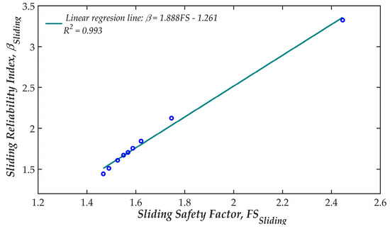
Figure 4.
Relationship between the reliability index and safety factor for sliding failure mode.
3.4. Reliability Analysis Using MCS
In the MCS, the input variables are generated following their statistical information, and the PF is then evaluated to classify events as failure or success after each sampling. The number of failures is counted and the failure probability in the simulation, Pf, is determined using Equation (14).
in which NMCS and Nfail are the simulation size and the number of failures occurring in the simulation, respectively. I(g(X) < 0) is an indicator function that reaches the value of unity if g(X) is less than zero and reaches the value of zero in other cases.
Additionally, the probability of failure in the MCS is significantly affected by the number of simulation. The COV of the failure probability based on the MCS, COVPf, is approximated from the number of simulation, NMCS, and the failure probability, Pf, as shown in Equation (15). Generally, the number of simulations, NMCS, should be greater than ten times the reciprocal of Pf (NMCS > 10/Pf) so that the COV of Pf estimated from the different MCS runs is less than 0.3 [33]. The relative error with a 95% confidence interval of binomial distribution of each simulation cycle is estimated with Equation (16) [27].
In Figure 5, the sensitivity of the realization number on the failure probability is analyzed for Onsan BRW. More than 40,000 simulations are necessary to reach a variation less than 0.3. In this study, the size of MCS is taken as 105 for the sliding reliability analysis. This size of simulation is also applied to other BRWs because the RI based on the FORM of the Onsan BRW is the largest among the nine BRWs. Meanwhile, based on the FORM results, the RIs for the overturning conditions are much higher than those of sliding, which is discussed in detail in Section 3.5. Consequently, the failure probability against overturning might be minor. By assuming the normal distribution, Figure 6 depicts the correlation between the smallest number of realizations to encounter at least 10 overturning failure events in the simulation and the expected RI. Particularly, if it is needed to reach a failure probability less than 10−6 (β > 4.75), 107 should be the smallest number of realizations applied. This example demonstrates one of the disadvantages of MCS in comparison with other methods like FORM and MVFOSM. Moreover, the results for overturning are not critical. Therefore, the RIs for overturning are assumed as the same as the results from FORM and MVFOSM in this work.
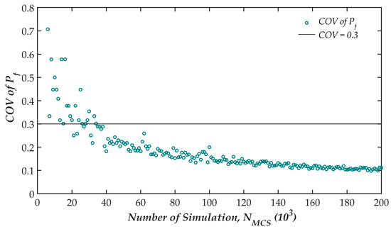
Figure 5.
Convergence of the Monte Carlo simulation (MCS) for sliding failure mode, (Onsan BRW).

Figure 6.
Relationship between the smallest number of simulations and the expected reliability index in MCS.
Figure 7 illustrates the histogram of the sliding FS (FSSliding) of the Onsan BRW compared with unity. The histogram shows a long tail on the right that declares that the distribution of the results is not symmetric even though the involved variables are considered as symmetric distributions. In these cases, the procedure proposed by Allen et al. [34], in which the sliding PF is plotted with the standard normal variable, can be applied to estimate the RI from the PF based on the MCS, as shown in Figure 8. The point at which the PF takes the zero value shows the negative RI. On the other hands, the point where performance line intersects with the horizontal axis illustrates the mean value of the PF. With the normal distributions, the slopes of the lines indicate the standard deviation of the PF. Finally, the RIs based on the three methods are plotted in Figure 9 for the sliding and overturning conditions. The results are discussed in detail in Section 3.5.
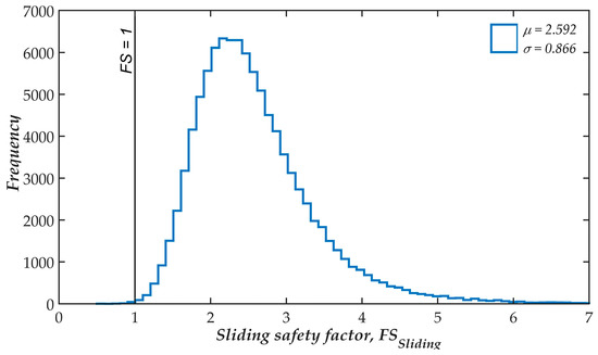
Figure 7.
Histogram of the sliding safety factor in the case of Onsan breakwater.
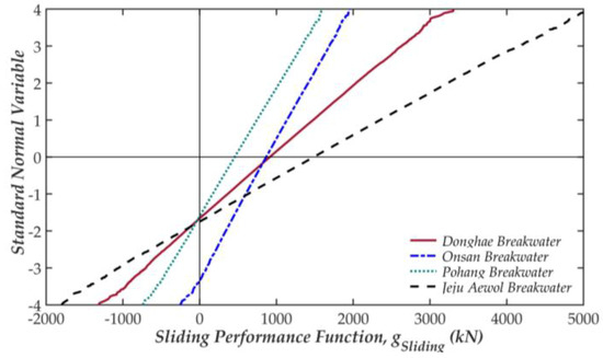
Figure 8.
Cumulative density of the sliding performance function (PF) in the standard normal space.
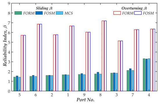
Figure 9.
Reliability indices for sliding and overturning failure modes (sorted by βSliding).
3.5. Discussion on Sliding and Overturning modes
A good agreement between the RIs for sliding and overturning failure modes by applying MVFOSM, FORM and MCS is achieved as shown in Figure 9. The MVFOSM corresponds better compared with FORM for the overturning conditions, implying that MVFOSM, the simplest method, should be applied for the linear PF. The average probability of overturning failure calculated using Equation (4) with the average of RIs is approximately 25 × 10−8. The probability of the overturning of a caisson around its heel is considerably small, as expected, implying that the failures would occur in the subsoil before the caisson itself would overturn [19]. The bearing capacity of the foundation is, therefore, examined in the next section.
Figure 9 distinctly indicates that the RIs of the sliding modes are considerably lower than those of the overturning mode. These results signify that a sliding event could more commonly occur during the lifetime of the structure. The sensitivity coefficients listed in Table 4 illustrates that the friction coefficient is the most critical factor in the resisting resultant in most of the BRWs. In contrast, the horizontal wave force controls the driving resultant. Based on this expression, the designer should find ways to reduce the horizontal wave force, such as applying a perforated or sloping top caisson, to mitigate the action of the ocean wave. On the other hand, the interaction conditions between the bottom of the caisson and the top of the rubble mound govern the friction coefficient; hence, this should be comprehensively inspected during the construction stage. Furthermore, friction enhancement materials should be utilized to reduce the width of the caisson, such as a rubber or bituminous material.
Additionally, although the plain concrete structure and filling material are considered to have the same bias factor, their effects on all the RIs vary widely due to the difference in the variable’s COV. It can be found that the variables contribute unequally to the FSs in reliability analysis, unlike the CDA. Moreover, some unsuitable points of the CDA can be observed in Figure 8. First, although the means of the sliding PFs are quite similar for the Onsan and Donghae BRWs, the estimated RIs show nearly twice the difference between the two. Second, the same RIs for the Donghae, Pohang, and Jeju Aewol BRWs emerged from different values of PFs, illustrating the inconsistency of the deterministic method.
The most likely linear relationship between the FS following the conventional design method and the resulting RIs is shown in Figure 4. This approximation could provide an initial estimation of the RI in feasibility studies where the FS is the final target.
4. Bearing Capacity of Foundation by Circular Slip Failure Analysis
4.1. Selection of Bishop’s Simplified Method
Failures in the foundations may be the results of insufficient soil bearing capacity with the wave action on the caisson structure and foundation. The damage related to the lack of bearing capacity might lead to the collapse of structures soon after substantial foundation failures. Circular slip failure is one of the prevailing damages that needs to be investigated to ensure the stability of structures [5,20].
In general, the safety of the BRW in preventing circular slip failure can be estimated based on the finite element analysis (FEA) or the limit equilibrium approach (LEA). In this study, the more classical method, the LEA, is applied because it is combined more readily with the probabilistic approach. In LEA, the failure mass corresponding to the range of candidate failure surfaces is divided into slices, and the FSs are estimated among the failure surfaces. The FS associated with each candidate failure surface is calculated by the ratio of the resisting force or moment to the mobilizing force or moment. As a result, the final FS of the slope stability is the smallest among those calculated. There are some LEAs in which the FSs are calculated with or without considering the inter-slice forces. Additionally, several methods evaluate the limit equilibrium against moments (Bishop’s simplified method) or forces (Janbu’s simplified method) or both moments and forces (Spencer, Morgenstern-Price’s approaches) [35].
In the Probabilistic Design Tools for Vertical Breakwaters (PROVERB), the bearing capacities are calculated using the upper bound (UB) theory [13]. The FS derived from the UB theory would locate on the unsafe side of the correct solution compared to both FEA and LEA. However, the FS values are slightly different between those methods. Several limit equations corresponding to the failure modes related to predefined surfaces or a set of surfaces based on the UB theory have been derived [36]. These equations with simplifying hypotheses are expressed in explicit functions, resulting in them being more easily solved in the reliability approach, i.e., easy to estimate the derivatives compared with those based on FAE and LEA. However, PROVERB also recommends that more sophisticated methods should be performed, such as slip circle analysis, according to Bishop or FEA during the detailed design process.
Kobayashi et al. [20] performed several extensive bearing capacity tests of rubble mounds, using such equipment as the tri-axial apparatus, in both a large-scale and a centrifuge model test in the laboratory and field tests and investigations of the behavior of actual gravity structure. The authors suggested that the bearing capacity of a rubble mound, including the sub-soil under eccentric and inclined loads, should be calculated using the BSM [20]. Additionally, the BSM is recommended as the suitable method used in verifying the bearing capacity of a foundation, as required in the standard of Ministry of Land, Infrastructure, Transport and Tourism (MLIT) [29] in Japan (2009) and Coastal Engineering Manual (CEM 2011) [28] in the United States. Therefore, the BSM is combined with the MCS in this study to discover the bearing capacity of the rubble mound and sub-soil under induced eccentric and inclined loading conditions.
4.2. Performance Function and Involved Random Variables
The probabilistic approaches for analyzing the stability of the slopes have been studied for decades. Based on the MVFOSM and FORM, several researchers have proposed models to determine the critical failure surface corresponding to the minimum RI, similar to the system reliability of the slope [37,38]. Conversely, others have proposed models to investigate the stability of the slope using the Gaussian random field process combined with the MCS [33,39,40]. However, the aforementioned studies do not mention about the slopes induced eccentric and inclined loads like a rubble mound structures.
Rubble mound structures are impacted by not only the dead load of the caisson structures but also the wave force action on the caisson. In this study, the bearing capacity of the caisson foundation, assuming circular slip conditions, is investigated concerning uncertainties in both the soil strength and acting forces. A combination of horizontal and vertical wave forces leads to eccentric and inclined loads on the caisson section, and the rupture slip surface might not separately divide the solid concrete caisson in parts. Therefore, the equilibrium of the caisson structure and the candidate failure soil mass, including a part of the rubble mound and a part of the subsoil, are individually considered [13]. Initially, the forces acting on the caisson structure are combined as “equivalent resultants” that can be expressed by the three parameters depicted in Figure 10: a horizontal force, Fh, at the top surface of the rubble mound; vertical force, Fu; and the distance of the vertical force to the harbor side heel, Bz. The equivalent resultants are then transmitted as reaction forces to the slope including the rubble mound and subsoil to determine the critical failure surface.
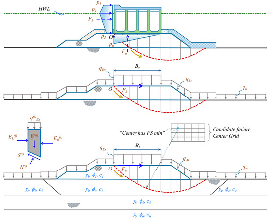
Figure 10.
Mechanism applied to estimate the PF against bearing capacity using a combination of Bishop’s simplified method and MCS.
Out of many slice methods, the BSM is a well-known selection in the stability analysis of slopes. In this approach, it is assumed that the resultants of the inter-slice forces are horizontal, i.e., the inter-slice shear forces are ignored. In that case, the FS is evaluated as the moment equilibrium around the center of the circular failure surface [41]. The FS can be determined using Equation (17), consequently, the PF in the reliability analysis based on the BSM is addressed in Equation (18). Therefore, the failure would occur when the PF is less than zero (or FS < 1) and vice versa.
In Equation (17), w′ and w are the effective weight and total weight of the comprising slice segment, respectively. qEx is the surcharge load distributing on the slice in the vertical direction. Fh and a correspond to the horizontal wave force and its lever arm about the failure center. c is the apparent cohesion of soil (or undrained shear strength in case of cohesive soil) while φ is the friction angle of soil along the base surface of each slice. s is the width of each slice. Finally, θ is the inclination angle, horizontal to the base surface. The studied variables, X, is shown as a vector of the involved variables in Equation (18). In the BSM, the FS is defined by a nonlinear and implicit equation; therefore, the FS is approximated with several iterative steps to reach the acceptable tolerance.
For each sampling of the MCS process, the FS of each trial failure surface is evaluated, and the smallest FS among the numerous candidate failure surfaces is considered as the final FS of the sampling. The effective dead load, wave forces acting on the caisson within each sampling are converted to the corresponding equivalent resultants, as in the previous discussion. In turn, the resultant is transposed to the rubble mound to estimate the FS using BSM. For each sampling, the FS is compared to unity as the margin between safety (FS ≥ 1) and failure (FS < 1) state. The number of failures occurring throughout the simulation is then utilized to estimate the failure probability.
In the present study, not only uncertainties explored in the sliding and overturning conditions but also the strength parameters of each soil layer are considered as random variables. The nominal soil properties of each layer are determined from the field investigation. Afterward, the mean of soil properties can be approximated based on the bias factor λ of each uncertainty, as shown in Table 5.

Table 5.
Statistical properties of foundation materials applied in bearing capacity analysis.
In most cases of geotechnical engineering, the parameters used in design may not be similar to their mean value. Therefore, the bias factors should be used to compensate for this difference. This gap can be caused by several reasons. First, some equations used in the design formulae do not always reflect exactly situation, i.e., biased phenomenon. Second, the result of the FS might have different shapes compared with those of the input variables, i.e., the dissimilar shapes of the density functions leading to a shift in the mean values.
Rubble mound structures generally consist of a homogeneous wide-graded mass of stone used to support a gravity structure. Previously, the strength properties of rubble mound material were well-defined based on various stability experiments, such as large-scale model, centrifuge and field loading tests [20]. By following that research, MLIT (2009) specified the shear strength parameters as 20 kN/m2 for the apparent cohesion and 35° for the internal friction angle for typical rubble materials supporting the eccentric and inclined loads as standard values. Various geotechnical parameters of rubble mounds and the subsoil were investigated in PROVERB (2001), where the soil strength properties were assumed as either the normal or lognormal distribution. However, the unit weights of the rubble mound and the subsoil were treated as deterministic variables [13]. In this work, when analyzing the bearing capacity of the foundation, both the unit weight of the rubble mound and subsoils are considered as random variables, similar to the sliding and overturning states.
In this study, the friction angle, undrained shear strength, and the unit weight of the rubble mound and subsoils are assumed to be unbiased (the mean of bias factors is unity) and exhibiting normal distribution for simplicity. The variation in the friction angle and the undrained shear strength is considered to have a value of 0.1 to account for the uncertainty in the estimated characteristic values. Notably, the variation in the subsoil density is less than the rubble mound density. Therefore, a slightly lower COV for the rubble mound is selected compared with that of the subsoil density. The stochastic information is summarized above in Table 5.
4.3. Result and Discussion of Bearing Capacity Analysis
Figure 11 presents an example of a failure event (FS less than unity) of the Gamcheon breakwater in a sampling. The safety factors are evaluated within the trial center grid consisting of 625 (25 × 25) points. The contour located in the upper part of the figure shows the convergence of the FSs in the estimation process. The blue line illustrates the most critical failure surface with a safety factor of 0.95, in which the failure mass consists of both rubble mound and subsoil portions.
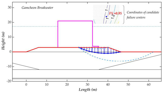
Figure 11.
Bearing capacity analysis applying Bishop’s simplified method (BSM) conjugated with MCS.
The nonlinear relationship between PF (through FS) and the standard normal variable is plotted in Figure 12 for the bearing capacity of foundations. The RI, in this case, should be determined from the points at which PF equals to zero (FS = 1) rather than inversion of the cumulative density function of the normal distribution. The results have illustrated that the MCS should be the most relevant approach when reliability analysis is applied to assess the bearing capacity of the foundation. Moreover, the point where the performance line is zero (FS = 1) provides a negative RI. Meanwhile, the mean value of PF is indicated when the standard normal variable equals zero.
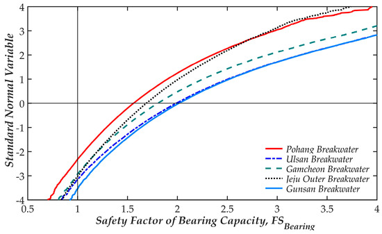
Figure 12.
Cumulative density of the bearing capacity safety factor of foundation in the standard normal space.
Furthermore, Figure 12 demonstrates that the CDA may be unsuitable when compared with the reliability methods in the stability assessment of BRWs. First, although the mean values (intersect points of the performance function with the horizontal axis) of the safety factor are different, some estimated RIs are quite similar. For example, for the Jeju Outer, Gamcheon and Ulsan BRWs, the means of the safety factors are obtained corresponding to 1.622, 1.727 and 1.897, but the estimated RIs are all approximately 3.3. Second, the results of RIs that vary from 2.658 (Pohang case) to 3.769 (Gunsan BRW) corresponding to the failure probability of 0.01 and 0.0002 show a large difference. The huge variation of failure probabilities (50 times of difference) illustrates the inconsistent safety level of the BRWs achieved using CDA.
Additionally, the meaningful results of the nine BRWs and the corresponding errors of the MCS estimated using Equation (16) with the generation size of one hundred and fifty thousand are presented in Table 6. The maximum error of 0.37% (COVPf ≈ 0.18) in the Gunsan case proves that the chosen size of simulation is suitable. Although all studied variables are assumed as normal distributions, the outcome of the FSs reveals a skewed distribution, as in the example shown in Figure 13 for the Gamcheon BRW. The skewness implies the asymmetry of the probability density function of the PFs, while a normal distribution (totally symmetric) would show a skewness value. The positive skew coefficients in all the studied cases imply that the PF’s distribution have a longer tail on the right compared with that on the left. This phenomenon reflects the nonlinear relationship of the safety factor with all the involved variables in the BSM. Additionally, the positive skewness instances are more densely located on the left side of the mean value. This result demonstrates that the safety factors of the reliability analysis are predominantly distributed below the mean value.

Table 6.
Results of the bearing capacity safety factor using Monte Carlo simulation.
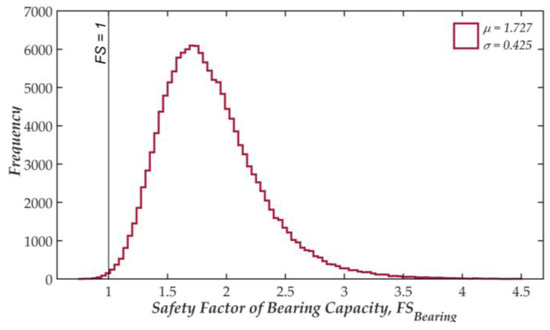
Figure 13.
Histogram of the bearing capacity safety factor of foundation (Gamcheon BRW).
Figure 14 presents the reliability index of the nine BRWs with respect to the three overall failure modes, including sliding, overturning, and foundation. Except Onsan case, which has lowest reliability index for foundation bearing capacity, the eight breakwaters have the smallest RIs for the sliding mode. Meanwhile the largest value of RIs are always for overturning mode. Notably, the Onsan BRW shows the remarkably low design wave height compared with the others, while the height of rubble mound is about a half of the water depth. These special features may reduce the wave forces on the caisson, meanwhile the high rubble mound may face a frequent failure. The average RI values of the nine BRWs are approximately 1.89 (Pf ≈ 0.0417) and 3.24 (Pf ≈ 0.0028), corresponding to the sliding state and failure occurrence in the foundation. Thereby, under similar service conditions, sliding failures might be observed much more frequently (about 15 times) than foundation failures. However, lower failure probability for sliding state in comparison with failures in foundation does not suggest that sliding damages will always take place before failures occurring in the rubble mound or subsoil—sliding failures are merely more common among the three overall stability conditions.

Figure 14.
Reliability index in different overall failure modes of BRWs (sorted by βSliding).
5. Conclusions
The present study focuses on the evaluation of the three most significant failures related to the overall stability of typical Korean vertical composite breakwaters using reliability approaches. Three primary sources of uncertainties are considered to clarify the variables’ sensitivity to the safety of breakwaters. The results presented in this work have provided the following conclusions.
First, among the three overall breakwater failure modes, the sliding mode is the most frequent failure state, so any such damage is a priority that needs to be surveyed to determine an appropriate width of caisson sections. Additionally, overturning may be rare in a breakwater failure because a remarkably low failure probability is obtained (25 × 10−8).
Second, in the most critical failure mode, the sliding state, the friction coefficient, and horizontal wave force contribute much more significantly to the safety of a breakwater in comparison with other concerned uncertainties.
Third, the results of the three methods, MVFOSM, FORM and MCS, applied to explicit performance functions, agree well, validating that these methods could be performed to conduct a reliability-based analysis for sliding and overturning. However, the simpler methods, i.e., MVFOSM or FORM, should be applied for the explicit definition of performance functions. Furthermore, implicit or nonlinear problems like the evaluation of breakwater’s foundation failure can be solved by applying reliability methods such as MCS.
Finally, a reliability analysis can overcome the drawbacks of the conventional deterministic design approach to provide a more consistent safety level of breakwaters. Additionally, it is expected that the reliability index of a breakwater against sliding state can be estimated from the results of the conventional deterministic design, i.e., the safety factor using the proposed linear regression line.
Author Contributions
Conceptualization, J.H., D.K. and N.S.D.; Methodology, N.S.D., J.H. and D.K.; Software, N.S.D and V.H.M; Validation, J.H., N.S.D., K.K. and V.H.M.; Formal analysis, J.H., N.S.D, and V.H.M; Resources, J.H. and K.K.; Writing-Original Draft Preparation, N.S.D, V.H.M and J.H.; Writing—Review and Editing, J.H., N.S.D., and V.H.M; Supervision, J.H. All authors have read and agreed to the published version of the manuscript.
Funding
This research was funded by the Ministry of Oceans and Fisheries, Korea, grant number 20180323.
Acknowledgments
This research was a part of the project entitled ‘Development of Design Technology for Safe Harbor from Disasters’ funded by the Ministry of Oceans and Fisheries, Korea.
Conflicts of Interest
The authors declare no conflict of interest.
References
- Goda, Y. Random Seas and Design of Maritime Structures; University of Tokyo Press: Tokyo, Japan, 2000. [Google Scholar]
- Bruining, J.W. Wave Forces on Vertical Breakwaters. Reliability of Design Formula. Master’s Thesis, Degree-Granting University, Delft, The Netherlands, 1994. [Google Scholar]
- Takahashi, S.; Shimosako, K.-I.; Kimura, K.; Suzuki, K. Typical failures of composite breakwaters in Japan. In Proceedings of the 27th International Conference on Coastal Engineering (ICCE), Sydney, Australia, 16–21 July 2000; pp. 1899–1910. [Google Scholar]
- Takagi, H.; Esteban, M.; Shibayama, T. Stochastic Design of Caisson Breakwaters: Lessons from Past Failures and Coping with Climate Change; Elsevier Inc.: Amsterdam, The Netherlands, 2015; pp. 635–673. [Google Scholar] [CrossRef]
- Oumeraci, H. Review and analysis of vertical breakwater failures—Lessons learned. Coast. Eng. Spec. Issue Vert. Breakwaters 1994, 22, 3–29. [Google Scholar] [CrossRef]
- Kim, T.-M.; Takayama, T. Improved evaluation of the expected sliding distance of a caisson and practical parameters of uncertain factors. In Proceedings of the 2nd International Conference (Asian and Pacific Coasts, 2003), Makuhari, Japan, 29 February–4 March 2004; pp. 1–16. [Google Scholar] [CrossRef]
- Ministry of Oceans and Fisheries. Harbor and Fishing Port Design Standards; Ministry of Oceans and Fisheries: Seoul, Korea, 2014.
- Low, B.K.; Phoon, K.K. Reliability-based design and its complementary role to Eurocode 7 design approach. Comput. Geotech. 2014, 65, 30–44. [Google Scholar] [CrossRef]
- Van der Meer, J.W. Rock slopes and gravel beaches under wave attack. Ph.D. Thesis, Degree-Granting University, Delft, The Netherlands, 1988. [Google Scholar]
- Christiani, E. Application of Reliability in Breakwater Design. Ph.D. Thesis, Hydraulics & Coastal Engineering Laboratory, Department of Civil Engineering, Aalborg University University, Aalborg, Denmark, 1997. [Google Scholar]
- Burcharth, H.F. Introduction of partial coefficients in the design of rubble mound breakwaters. In Proceedings of the Conference on Coastal Structures and Breakwaters, ICE, London, UK, 1 January 1992; pp. 543–565. [Google Scholar]
- Burcharth, H.F.; Sorensen, J.D. Design of vertical wall caisson breakwaters using partial safety factors. In Proceedings of the 26th Conference on Coastal Engineering, Copenhagen, Denmark, 22–26 June 1998; pp. 2138–2151. [Google Scholar]
- Oumeraci, H.; Kortenhaus, A.; Allsop, W.; de Groot, M.; Crough, R.; Vrijling, H.; Voortman, H. Probabilistic Design Tools for Vertical Breakwaters; Swets & Zeitlinger, B.V.: Lisse, The Netherlands, 2001.
- Kim, S.W.; Suh, K.D. Application of reliability design methods to Donghae Harbor breakwater. Coast. Eng. J. 2006, 48, 31–57. [Google Scholar] [CrossRef]
- Kim, S.W.; Suh, K.D. Reliability analysis of breakwater armor blocks: Case study in KOREA. Coast. Eng. J. 2010, 52, 331–350. [Google Scholar] [CrossRef]
- Hong, S.Y.; Suh, K.D.; Kweon, H.M. Calculation of expected sliding distance of breakwater caisson considering variability in wave direction. Coast. Eng. J. 2004, 46, 119–140. [Google Scholar] [CrossRef]
- Kim, S.W.; Suh, K.D. Evaluation of target reliability indices and partial safety factors for sliding of caisson breakwaters. J. Coast. Res. 2011, 64, 622–626. [Google Scholar]
- Takayama, T.; Ikeda, N. Estimation of Sliding Failure Probability of Present Breakwaters for Probabilistic Design; Ministry of Transport: Yokosuka, Japan, 1992.
- Goda, Y.; Takagi, H. A Reliability design method of caisson breakwaters with optimal wave heights. Coast. Eng. J. 2000, 42, 357–387. [Google Scholar] [CrossRef]
- Kobayashi, M.; Terashi, M.; Takahashi, K. Bearing Capacity of a Rubble Mound Supporting a Gravity Structure; Ministry of Transport: Yokosuka, Japan, 1987.
- Takagi, H.; Esteban, M. Practical methods of estimating tilting failure of caisson breakwaters using a Monte-Carlo simulation. Coast. Eng. J. 2013, 55. [Google Scholar] [CrossRef]
- Shimosako, K.A.T.S. Reliability Design Method of Composite Breakwater Using Expected slIding Distance; Ministry of Transport: Yokosuka, Japan, 1998; pp. 4–30.
- Hanzawa, M.; Sato, H.; Takahashi, S.; Shimosako, K.; Takayama, T.; Tanimoto, K. New stability formula for wave-dissipating concrete blocks covering horizontally composite breakwaters. In Proceedings of the Coastal Engineering Conference, Orlando, FL, USA, 2–6 September 1996; pp. 1665–1678. [Google Scholar]
- Cornell, C.A. A probability-based structural code. ACI J. 1969, 66, 974–985. [Google Scholar] [CrossRef]
- Ang, A.H.; Tang, W.H. Probability Concepts in Engineering Planning and Design, Volume 2: Decision, Risk, and Reliability; John Wiley & Sons: New York, NY, USA, 1984. [Google Scholar]
- Hasofer, A.M.; Lind, N.C. Exact and Invariant Second-Moment Code Format. ASCE J. Eng. Mech. Div. 1974, 100, 111–121. [Google Scholar]
- Haldar, A.; Mahadevan, S. Probability, Reliability and Statistical Methods in Engineering Design; John Wiley: Hoboken, NJ, USA, 2000. [Google Scholar]
- United States Army Corps of Engineers. Coastal Engineering Manual Part VI: Design of Coastal Project Elements (EM 1110-2-1100); Books Express Publishing: Washington, DC, USA, 2011; Volume 1100-2-110.
- MLIT. Technical standard and commentaries for port and harbor facilities in Japan; Ministry of Land, Infrastructure, Transport and Tourism (MLIT); Ports and Harbors Bureau: Tokyo, Japan, 2009.
- Goda, Y. New wave pressure formulae for composite breakwaters. In Proceedings of the Proceedings International Conference Coastal Engineering (ICCE), Copenhagen, Denmark, 24–28 June 1974; pp. 1702–1720. [Google Scholar]
- Van der Meer, J.W.; D’Angremond, K.; Juhl, J. Probabilistic calculations of wave forces on vertical structures. In Proceedings of the International Conference Coastal Engineering (ICCE), Kobe, Japan, 23–28 October 1994; American Society of Civil Engineers: Reston, VA, USA, 1994; pp. 1754–1767. [Google Scholar]
- Vrijling, J.K. Evaluation of uncertainties and statistical descriptions. In Proceedings of the Task 4 Workshop Hannover, MAST III, PROVERBS-Project: Probabilistic Design Tools for Vertical Breakwaters, Hannover, Germany, September 1996. [Google Scholar]
- Ching, J.; Phoon, K.K.; Hu, Y.G. Efficient evaluation of reliability for slopes with circular slip surfaces using importance sampling. J. Geotech. Geoenviron. Eng. 2009, 135, 768–777. [Google Scholar] [CrossRef]
- Allen, T.M.; Nowak, A.S.; Bathurst, R.J. Calibration to Determine Load and Resistance Factors for Geotechnical and Structural Design. Transp. Res. Circ. 2005. [Google Scholar] [CrossRef]
- Duncan, J.M.; Wright, S.G. The accuracy of equilibrium methods of slope stability analysis. Eng. Geol. 1980, 16, 5–7. [Google Scholar] [CrossRef]
- Vrijling, J.K. Probabilistic Design Tools for Vertical Breakwaters. Final Report. Volume IId. Probabilistic Aspects; Swets & Zeitlinger, B.V.: Lisse, The Netherlands, 1999.
- Bhattacharya, G.; Jana, D.; Ojha, S.; Chakraborty, S. Direct search for minimum reliability index of earth slopes. Comput. Geotech. 2003, 30, 455–462. [Google Scholar] [CrossRef]
- Chowdhury, R.N.; Xu, D.W. Geotechnical system reliability of slopes. Reliab. Eng. Syst. Saf. 1995, 47, 141–151. [Google Scholar] [CrossRef]
- Cho, S.E. Effects of spatial variability of soil properties on slope stability. Eng. Geol. 2007, 92, 97–109. [Google Scholar] [CrossRef]
- Griffiths, D.V.; Fenton, G.A.; Denavit, M.D. Traditional and advanced probabilistic slope stability analysis. In Proceedings of the Geotechnical Special Publication, Denver, CO, USA, 18–21 February 2007; p. 19. [Google Scholar]
- Bishop, A.W. The use of the slip circle in the stability analysis of slopes. Geotechnique 1955, 5, 7–17. [Google Scholar] [CrossRef]
© 2020 by the authors. Licensee MDPI, Basel, Switzerland. This article is an open access article distributed under the terms and conditions of the Creative Commons Attribution (CC BY) license (http://creativecommons.org/licenses/by/4.0/).