1. Introduction
The hydrodynamic noise level of underwater vehicles, such as submarines, torpedoes, and underwater unmanned vehicles (UUVs) is significantly related to their detection opportunities. The normal methods to reduce the hydrodynamic noise are based on line-type optimization, the utilization of a sound absorption layer, and material selection. Little research has been focused on flow control. Inspired by owls, which can fly silently in the night, scientists have tried placing serrations on the leading edge to enhance lift and suppress flow separation in the aerodynamic field, especially on airplanes.
The notion that serrations have an important function in noise reduction was confirmed by Matthias Weger when he investigated the serrations on complete wings and on the 10th primary remiges of seven owl species [
1]. Since the unsteady blade forces are of lower magnitude for a fan with sinusoidal leading edges than for a fan with straight leading edges [
2], and torque fluctuations are significantly suppressed due to the passive flow control strategies implemented in the optimized vertical axis wind turbine model [
3], even the effect of the stagnation point on the flow in front of the leading edge is observed to reduce drastically in the case of serrations [
4]. Therefore, scientists now believe that leading-edge serrations can reduce noise.
Some theories have been believed to reveal the mechanism of noise reduction through leading-edge serrations. First, the serrated wing can passively control the laminar-turbulent transition to suppress high-frequency eddies, leading to sound suppression [
5]. Second, counter-rotating vortex pairs are generated due to the existence of serrations, which suppress the flow separation, especially in the regions near the peak-serration sections [
6]. Third, the leading-edge serrations can reduce the unsteady pressure magnitude near the leading edge, reduce the spatial coherence of the source region, and increase spanwise phase variation [
7]. Fourth, the leading-edge serrations serve as flow-stabilizing devices [
8]. All of these factors are thought to contribute to the effect of noise suppression.
To obtain the optimum noise reduction, scientists have investigated the relationship between the level of noise reduction and the parameters of the leading-edge serrations, such as the wavelength, the amplitude, and so forth, because the ratios between the integral scales of upstream turbulent disturbances and the serration amplitude/wavelength are important. Chaitanya proposed that when the spanwise separation distance between adjacent roots is less than twice the turbulence integral length scale, at least 3 dB of additional noise reduction can be achieved [
9]. Samion found that a noise reduction of up to 3.5 dB is obtained when the serrations are wider [
10]. Juknevicius suggested that the most effective leading-edge serrations should possess a large wavelength and small amplitude [
11]. Chaitanya found that when the transverse integral length scale is approximately one-fourth of the serration wavelength, the maximum noise reduction is obtained [
12]. Zhang found that the optimum airfoil performance within a wide attack angle range is acquired by reasonably designing the amplitude, wavelength, and shape of the protuberances [
13]. However, all of these research works are based on experiments or simulations, and the summarized laws are only correct under these conditions; they are not suitable for other situations. For example, Feinerman’s simple theory related to noise reductions for the oblique case is largely overpredicted [
14].
At the same time, other flow control techniques at the leading edge are proposed to obtain better noise reduction. The implementation of leading-edge blowing can successfully minimize the parallel blade–vortex interaction, and the vibration energy of the airfoil decreases by up to 12 dB
re M=0 [
15]. The blowing slot can form a strong and steady vortex, which can reduce the intensity and axial velocity excess in the core of the primary vortex [
16]. Leading-edge blowing generally increases the strength of the vortices, and may even cause premature vortex breakdown at moderate incidences [
17]. A small plate near the leading edge of the airfoil is set to circumvent the flow separation [
18]. The low-amplitude oscillating distributed surface perturbations can completely suppress the leading-edge separation bubbles [
19].
Casalino investigated the effect of sinusoidal serrations applied to the leading edge of the vanes of a realistic fan stage, and obtained some noise reductions when the undulation amplitude and wavelength were large enough compared to the integral scales of the impinging turbulence fluctuations [
20].
The listed results are mostly carried out in the aerodynamic field, and are only considered as possible references for the hydrodynamic field due to the differences between the two fields. First, the Reynolds number is larger in the water than in the air. An experiment inhibiting the flow separation by serrations at a low Reynolds number has been validated in the air [
21], and no turbulence or cavitation occurs. However, turbulence or cavitation is usually observed in the water because of the higher Reynolds number. Second, noise reduction is mostly considered in the low-frequency range, since low-frequency noise can propagate over a long distance in the water. However, noise reductions achieved by the use of leading-edge serrations are not significant at low frequencies; they are more significant in the mid-frequency range in the aerodynamic field [
22]. Third, air is a light medium, while water is a heavy medium. Their viscosities are also different. Therefore, the eddies formed in the water are not the same as those that form in the air. The noise-reduction mechanism in the water by leading-edge serrations may not be the same as that which occurs in the air.
Although many simulations and experiments show that noise reduction can be achieved by leading-edge serrations, Rao’s results show that the tradeoff between turbulent flow control and force production in the serrated model holds independently to wind-gust environments [
23]. Meanwhile, Wei experimentally investigated the hydrodynamic characteristics of hydrofoils with leading-edge tubercles in a water tunnel at a low Reynolds number of
Re = 1.4 × 10
4 [
24]. His research mainly focused on flow separation suppression, and did not focus on noise reduction. In addition, the primary instability of a squared leading-edge flat plate is reduced under a transition control method [
25]. Therefore, to obtain better hydrodynamic noise suppression using leading-edge serrations, we must investigate the effect of flow control and noise reduction together.
In this research, we placed the serrations on the leading edge of a sail hull on the SUBOFF model. Through the numerical simulation, we revealed the noise reduction mechanism through flow control by leading-edge serrations, especially at a high Reynolds number. Since the flow control mechanism occurs in the turbulent state, the results are more applicable to underwater vehicles. We have also summarized the parameters of the serrations, to achieve an optimum noise reduction. After that, we built two steel models according to the dimensions in the simulation. The experimental test was carried out in a gravity water tunnel. The simulated results were validated by the experiments. We believe that the results in this paper can provide a reference for the design of underwater vehicles with a low level of hydrodynamic noise.
3. The Description of the Model in the Numerical Simulation
3.1. The Research Model
SUBOFF is a specific model of submarine, which was jointly proposed by DARPA (Defense Advanced Research Projects Agency) and DTRC (David Taylor Research Center) [
29]. To reveal the phenomena of the horseshoe vortex, reduce the number of the grids, and save time with the numerical calculation, we have neglected some parts of the submarine body on the SUBOFF model. The selected object is the sail hull with part of the submarine body.
Since the horseshoe vortex is formed near the leading edge, developed at the bottom side, and dissipated at the tail of the sail hull, the flow at other parts of the SUBOFF model has no effect on the formation, development, and dissipation of the horseshoe vortex. Besides, the noise reduction is evaluated by the comparison between the original model and the model with the leading-edge serrations; the noise reduction is a relative value, not an absolute value. As long as the horseshoe vortex is formed, the results are adequate for the evaluation. Therefore, the other parts of the submarine body can be reasonable ignored.
The model, with a ratio of 1:48 and the length of 1.84 m (L), is shown in
Figure 2. The sail hull is also approximately considered to be the structure of an airfoil, of which the chord length is 0.184 m.
3.2. The Parameters of the Numerical Simulation
The turbulence equations are solved numerically using the finite volume method, which is realized by the FLUENT codes. The outside of the model is the calculation domain of the flow field, with the shape of a rectangle. The distance between the model and inlet flow and the model and outlet flow is 1 L and 2 L, respectively. The width of the flow field is six times the chord length. The height is three times the chord length. The boundary of the computational domain, including the inlet, the outlet, the plane of the object, and the regions of the outside boundary, are set as the velocity inlet, the pressure outlet, the symmetrical boundary conditions, and the solid wall boundaries. The velocity of the flow is 8.68 m/s.
The convection term is discretized by a second-order upwind scheme, whereas the diffusion term is discretized by a central difference scheme. The temporal term is discretized by a second-order implicit scheme, whereas the pressure–velocity coupling equation is solved using the PISO (Pressure-implicit with Splitting of Operators) method.
The SIMPLE (Semi-Implicit Method for Pressure Linked Equations) algorithm is the most widely used in flow field calculations in engineering. The PISO algorithm is an improvement of the SIMPLE algorithm. The difference between the SIMPLE algorithm and SIMPLEC algorithm is that only one prediction step and one correction step exist. The PISO algorithm includes one prediction step and two correction steps. After the completion of one-step correction, the information on the flow field is obtained. A second improvement is searched for, which can better satisfy the momentum equation and the continuity equation. The PISO algorithm uses the prediction–correction–recorrection steps, which can accelerate the convergence speed of the single-iteration step. The calculation speed is fast, and the solution efficiency is high. To solve the transient problem, the PISO algorithm has an obvious advantage. Therefore, we have chosen the PISO algorithm to solve the problem. This is also the calculation method recommended by FLUENT’s help documentation.
We have previously verified the wall-state function method combined with the RNG (Re-normalization Group) model for flow field steady-state calculation based on the PISO algorithm. We obtained different y+ values by changing the thickness of the first layer. Through the comparison between the numerically calculated results and experimental results, the appropriate range of y+ values is acquired
Table 1 shows the comparison between the numerical calculation and the experimental test of SUBOFF resistance at different
y+ values. When
y+ < 50, the value of the numerical calculation is the closest to that of the experimental test.
Subsequently, the submarine tail flow was carried out, as shown in
Figure 3. When
y+ < 50, the numerical simulation results are in good accordance with the experimental test values.
In the LES, when y+ < 50, we can obtain more accurate information regarding the flow field from the SUBOFF full-attachment model. Therefore, we have chosen y+≈35 for the numerical simulation.
The method of the wall function is combined with the RNG model to calculate the steady-state flow field, where
Re = 1.6 × 10
7. The mesh thickness of the first boundary layer, namely
, is 0.0001 m, which is obtained from Equation (21):
Considering time, cost, and computational power, we performed a steady-state grid-independent verification. We calculated the resistance value of the models with grid numbers of 1 million, 1.5 million, 2 million, 2.5 million, 3 million, 3.5 million, and 4 million. Through the comparison, we found that a grid number of 3 million obtains the appropriate resistance. Therefore, the grid number of the flow field calculation is 3 million. The transient simulation of the flow field was performed by the dynamic sublattice model in the LES.
Since the maximum frequency of the analysis is 2 kHz, the time step is determined to be 2.5 × 10⁻⁴ s according to Equation (22). The number of the sample is selected as 800 time steps for the calculation of the sound field.
To analyze the flow field and the sound field in detail, planes are set up as shown in
Figure 4. Plane A is in the longitudinal direction, and aligned with the center of the height of the sail hull. Plane B is also in the longitudinal direction, and aligned with the center of the thickness of the sail hull. Plane C is in the transverse direction, and aligned with the center of the length of the sail hull.
4. The Application of Leading-Edge Serrations
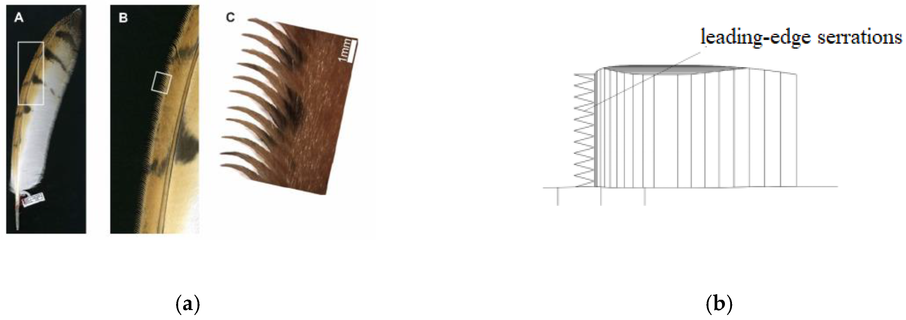
Figure 5 shows the structure of leading-edge serrations in owls. We designed the sail hull according to the structure seen in owls; that is, we created leading-edge serrations on the sail hull.
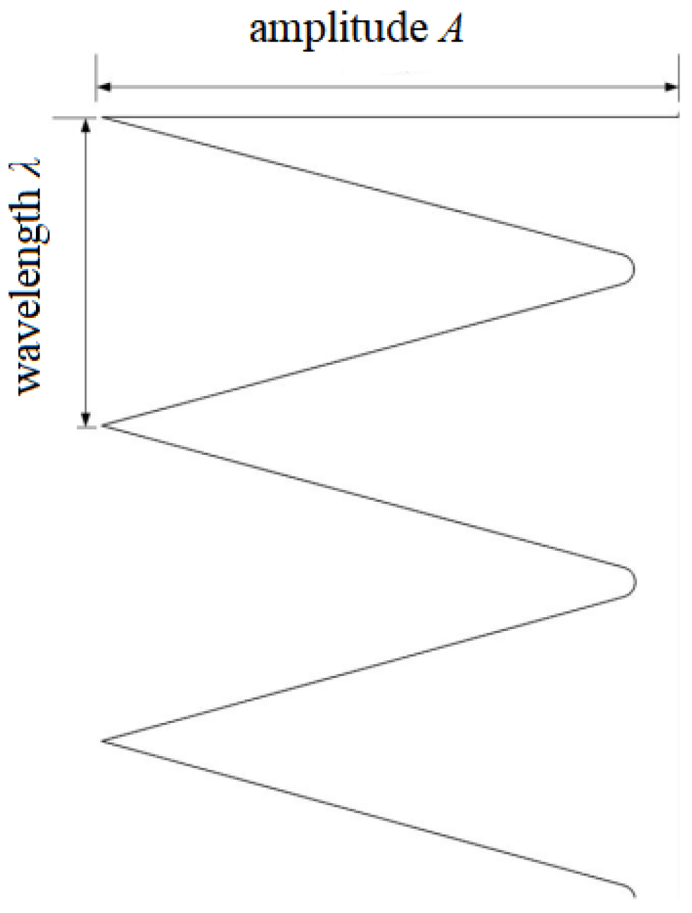
The geometric parameters of leading-edge serrations, the amplitude (A), and the wavelength (λ) are shown in
Figure 6. In this section, based on results from the aerodynamic field, we have selected an amplitude of 0.1c and a wavelength of 0.1h, where c is the chord length and h is the height of the sail hull.
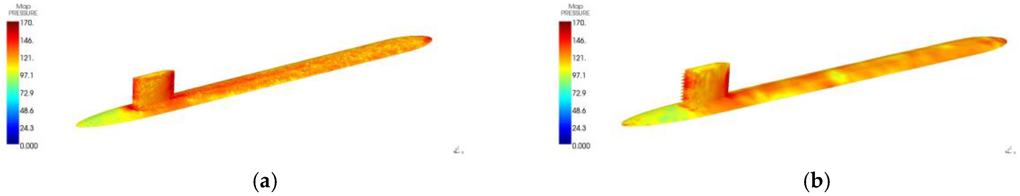
Figure 7 shows the surface pressure distribution comparison between the original model and the model with leading-edge serrations. We can see that the low-pressure area on both sides of the sail hull with leading-edge serrations becomes wider, and the minimum pressure is larger than that of the original model. The minimum pressure was increased by 22.4%. This phenomenon shows that the pressure gradient at the stagnation point of the sail hull is decreased, and the separation of the boundary layer is delayed.
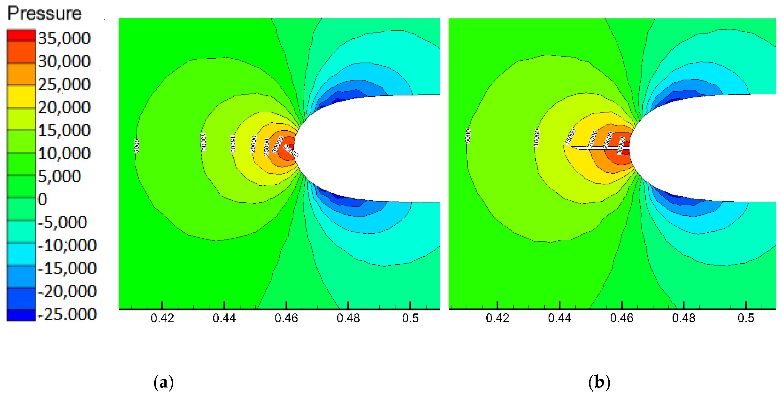
Figure 8 shows the pressure contour at Plane A of the two models. The horseshoe vortex is generated due to the pressure gradient at the junction between the leading edge of the sail hull and the submarine body. We can see that the maximum pressure at the junction between the sail hull and the submarine body becomes smaller after the placement of leading-edge serrations. The adverse pressure gradient also becomes smaller. Therefore, the formation of the horseshoe vortex has been influenced, such that the intensity of the horseshoe vortex will be reduced by leading-edge serrations.
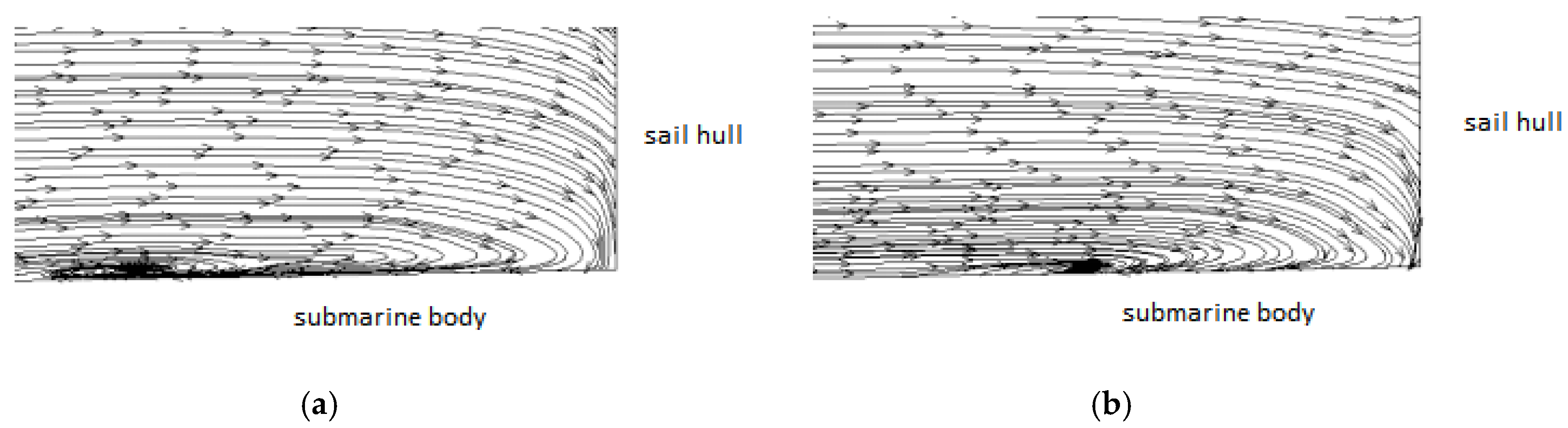
Figure 9 shows the streamlines at Plane B of the two models. As we know, the horseshoe vortex is formed at the leading edge of the sail hull, and then developed and dissipated. Therefore, the rotated streamlines show the origin of the horseshoe vortex, which exists in front of the leading edge of the sail hull. However, the vortex core becomes smaller and the adverse pressure gradient becomes even after leading-edge serrations are placed. This phenomenon confirms that leading-edge serrations reduce the pressure gradient and weaken the intensity of the horseshoe vortex.
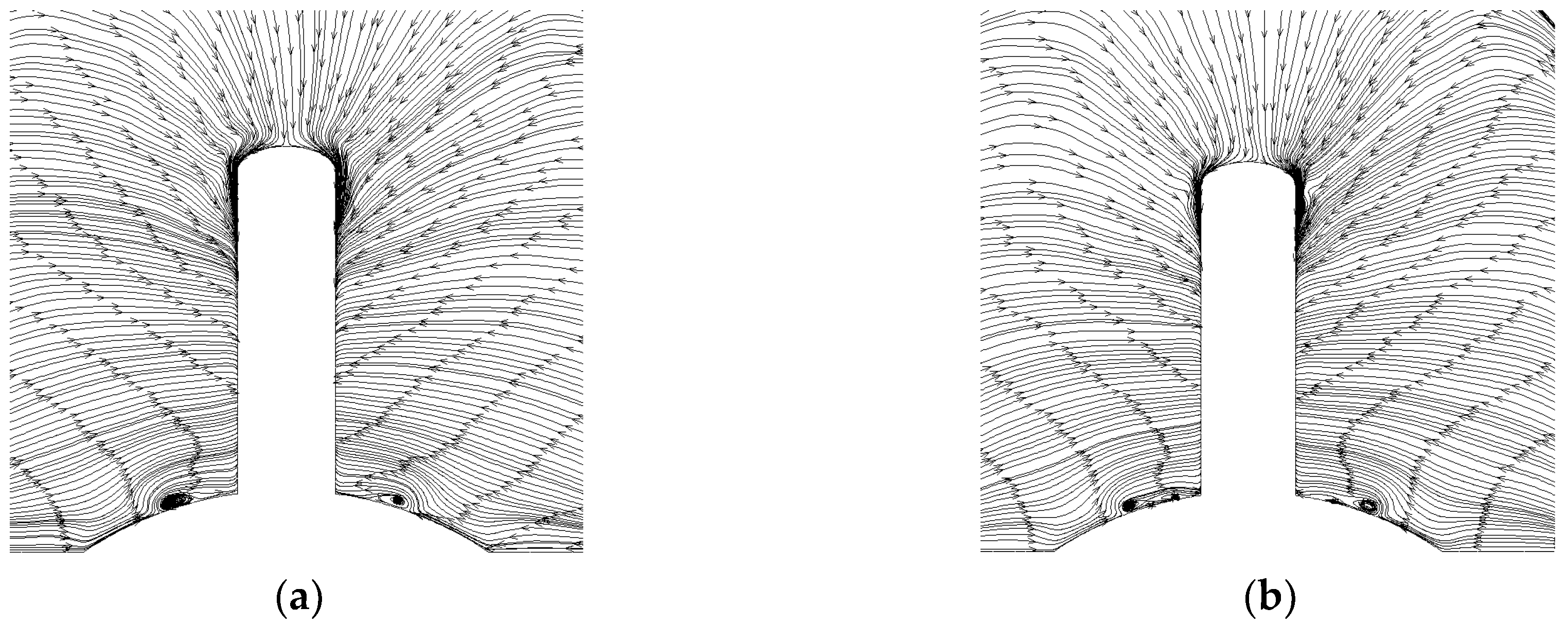
Figure 10 shows the streamlines at Plane C of the two models. The leading-edge serrations are similar to the flat plates in terms of the angle of attack. A pressure difference exists between the two sides. The water flows from the area of high pressure to the area of low pressure, and also runs along the flow direction. The resultant motion of these two factors formed a structure of spiral vortices, which are opposite to the rotation of the horseshoe vortex. Therefore, the intensity of the horseshoe vortex was weakened.
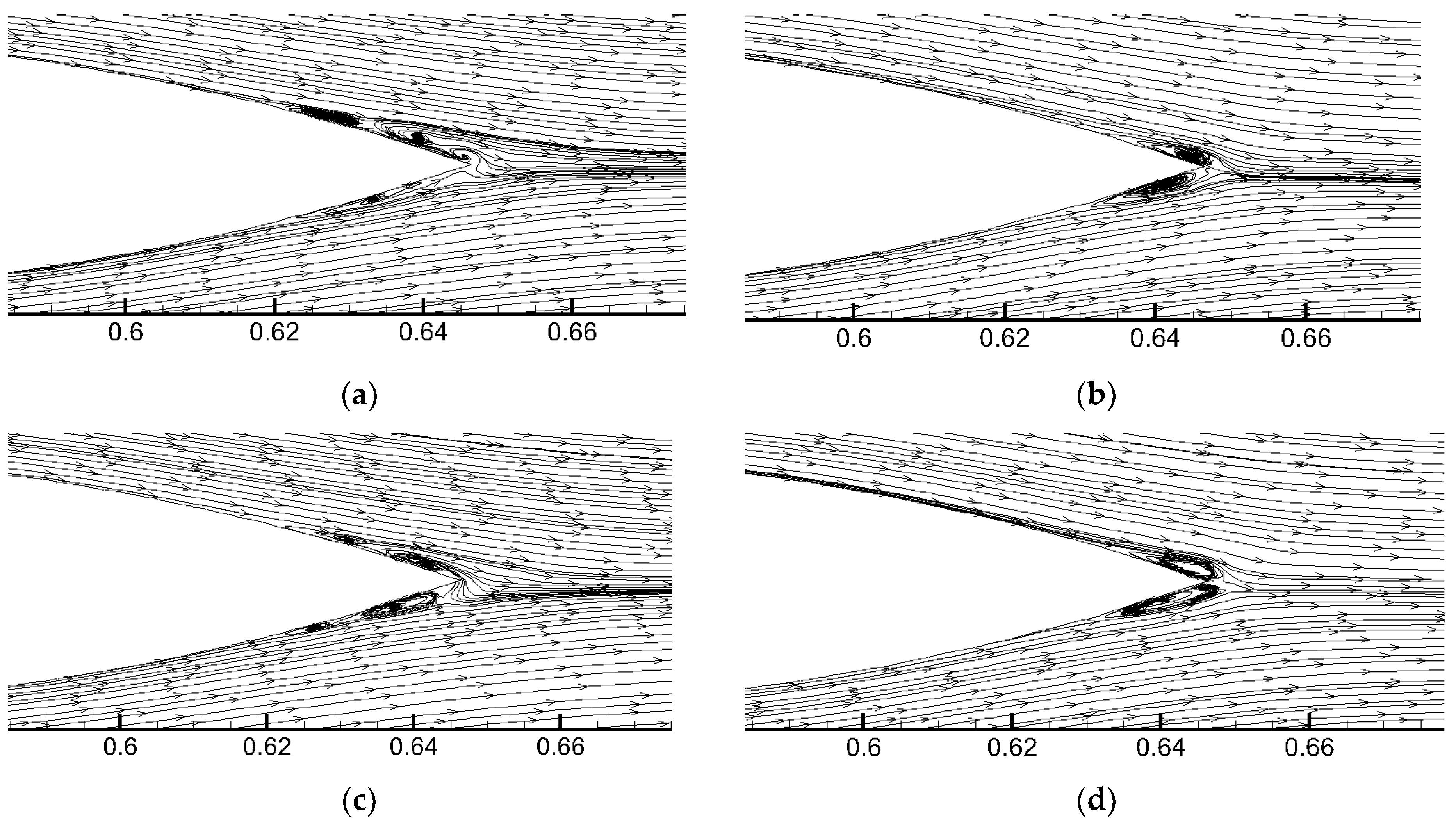
Figure 11 shows the streamlines at the trailing edge of the two models at different times. Through this comparison, we can see that the vortices generated by the boundary layer separation are formed at the position of
x = 0.62 m in the original model. On the other hand, the vortices generated by the boundary layer separation are formed at the position of
x = 0.63 m in the model with leading-edge serrations.
We may conclude that leading-edge serrations can inhibit boundary layer separation, even at the trailing edges of the sail hull, since leading-edge serrations are far away from the trailing edge of the model. The leading-edge serrations can also act as vortex generators, and inject outside flow energy into the boundary layer.
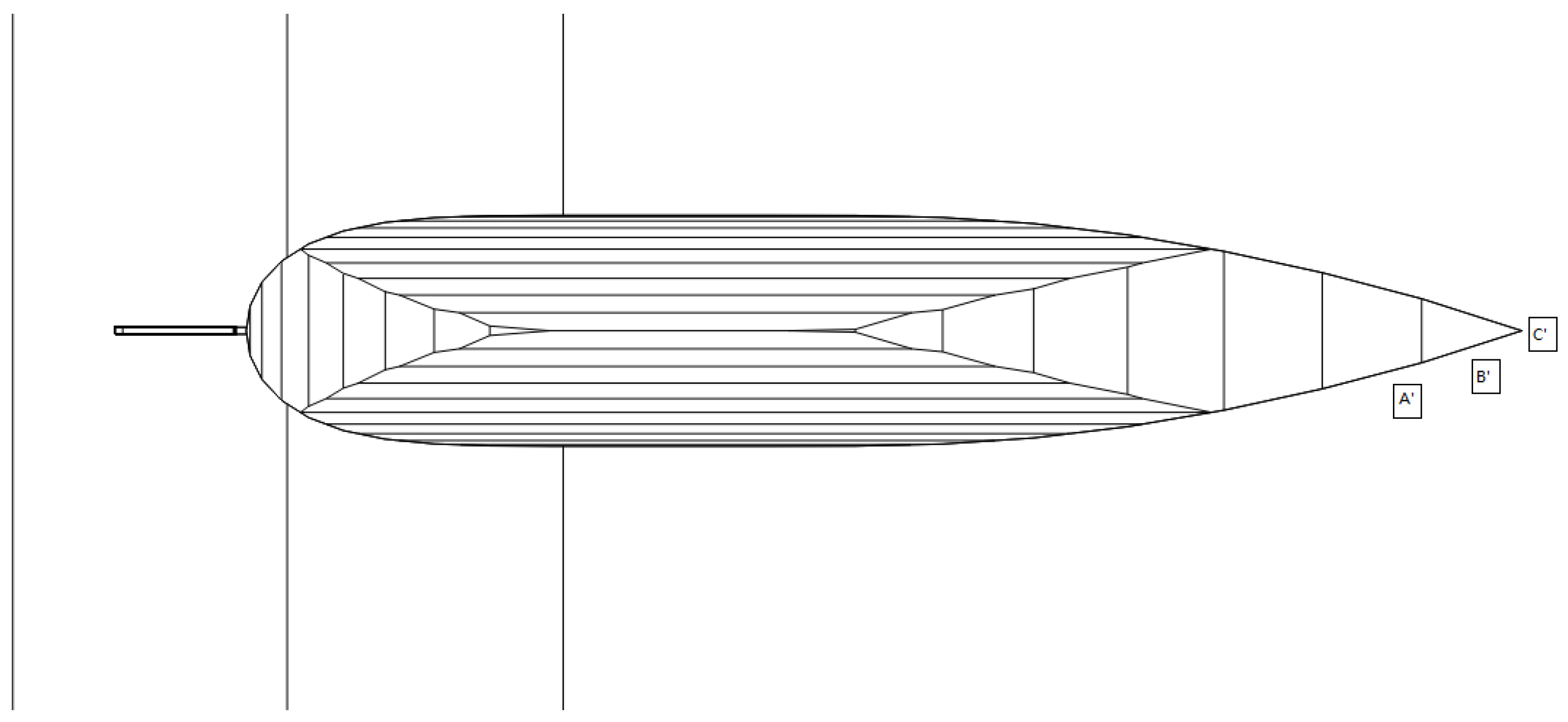
At the trailing edge of the sail hull at plane A, we have chosen three points: Point A’, Point B’, and Point C’. Point A’ and Point B’ are at a distance of 0.1c and 0.05c from the trailing edge, respectively. Point C’ is at the trailing edge.
Figure 12 is the schematic diagram of the three points in the sail hull.
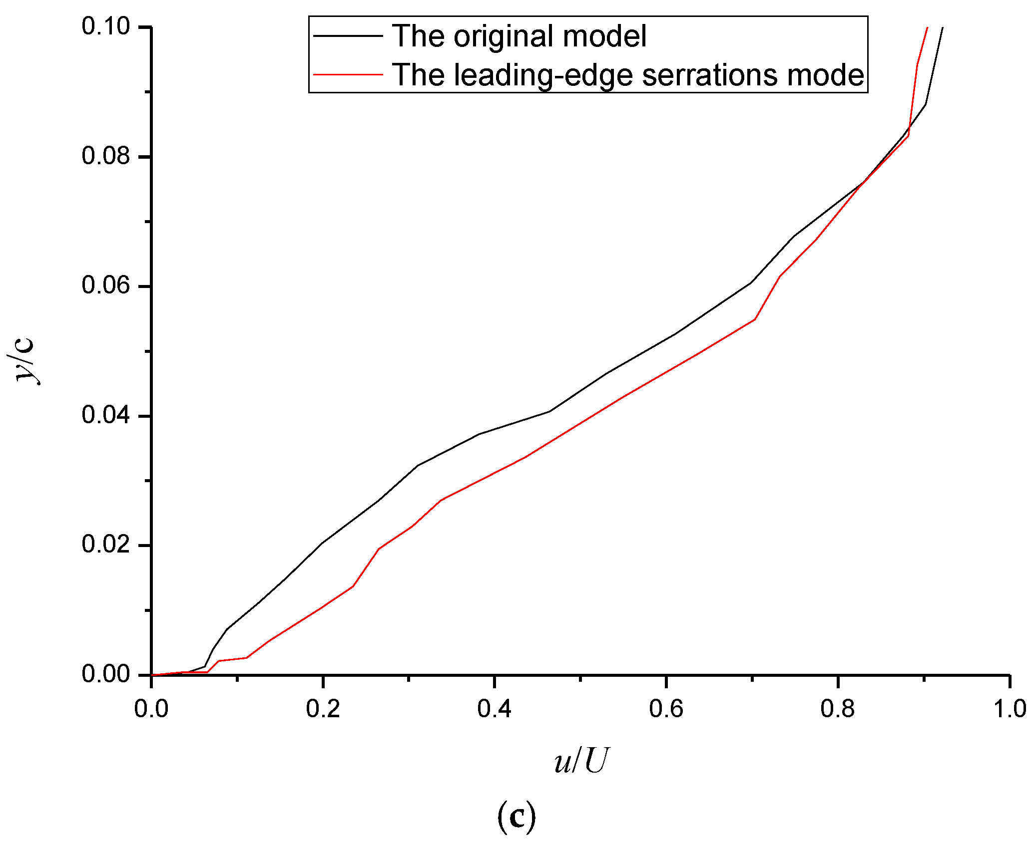
Figure 13 shows the boundary layer velocity distribution of the three points. The horizontal axis shows the ratio between the velocity and the incoming velocity (8.68 m/s). The vertical axis shows the ratio between the normal direction of the sail hull surface and the chord length of the sail hull.
At Point A’ and Point B’, a negative gradient at the wall velocity of the sail hull occurs in the original model. The velocity curve shows that the boundary layer separation occurs at the two points. However, no negative gradient occurs at the wall velocity of the model with leading-edge serrations. This phenomenon shows that boundary layer separation does not occur in the model with leading-edge serrations at these two points. Therefore, leading-edge serrations can effectively delay boundary layer separation at the trailing edge of the sail hull. At Point C’, no boundary layer separation occurs in either of the two models due to its position.
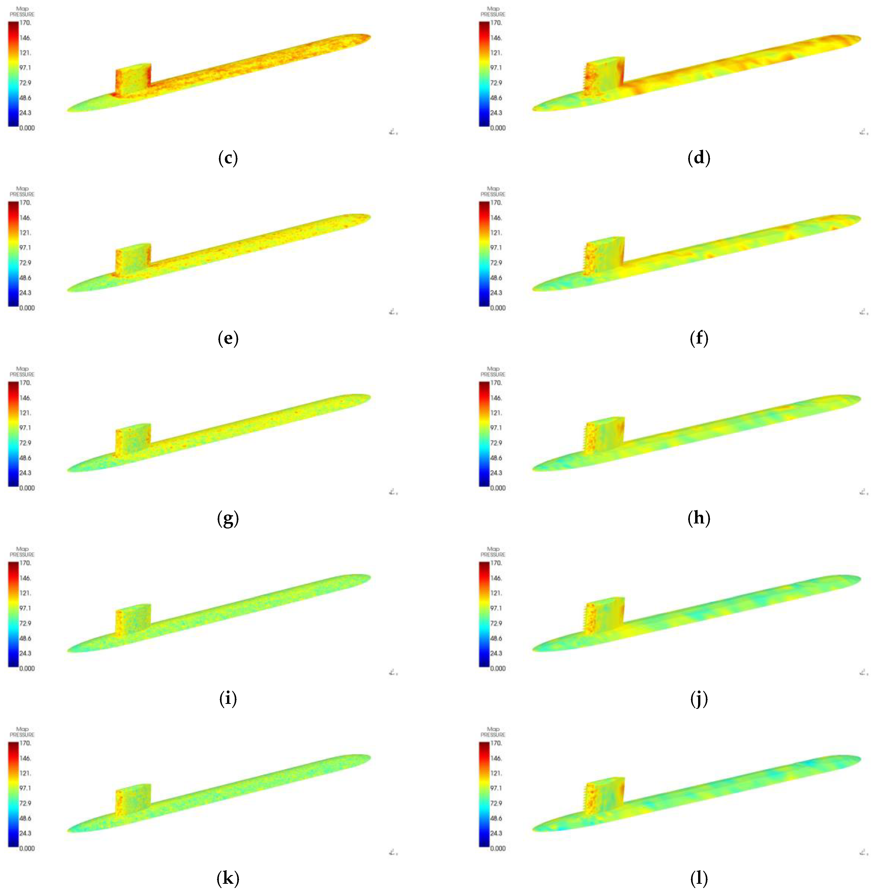
Figure 14 shows the fluctuation pressure contour at different frequencies of the original model and the model with leading-edge serrations. After the application of leading-edge serrations, the turbulent fluctuation pressure area caused by the horseshoe vortex on the surface of the sail hull and the submarine body is obviously reduced in the low-frequency range. This phenomenon further confirms that leading-edge serrations can weaken the intensity of the horseshoe vortex. Therefore, the low-frequency flow-induced noise from the excitation of the horseshoe vortex is weakened. At the same time, the intensive turbulent fluctuation pressure area at the trailing edge of the sail hull is also reduced in the low-frequency range. This phenomenon also demonstrates that leading-edge serrations can delay boundary layer separation, even if the leading-edge serrations are far away from the trailing edge. However, it should be noted that the presence of leading-edge serrations increases the leading-edge area of the sail hull. Since the leading-edge area is under high turbulent fluctuation pressure at each frequency, the flow-induced noise from the sail hull may be enhanced by leading-edge serrations in this case.
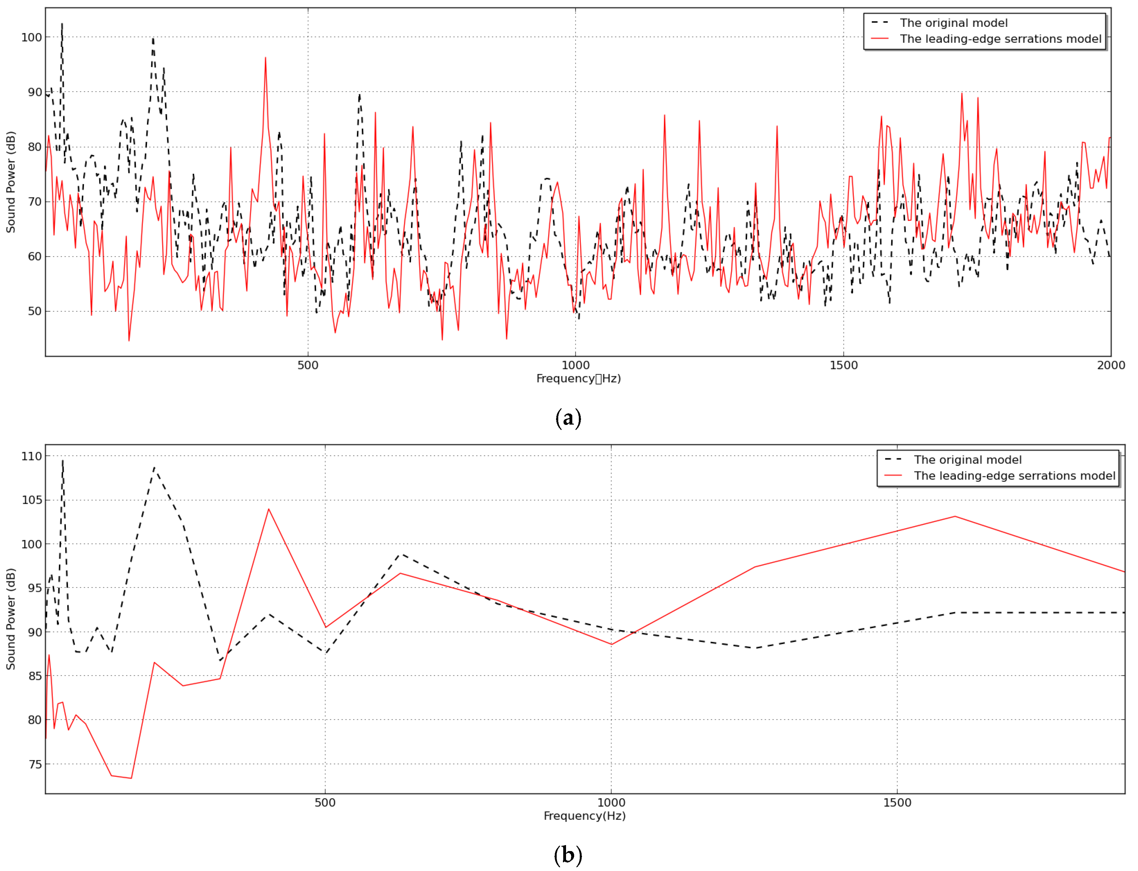
Figure 15 shows the comparison curve of the sound radiation power between the original model and the model with leading-edge serrations. In the low-frequency range, when
f <350 Hz, the sound radiation power from the model with leading-edge serrations is significantly lower than that of the original model. The two low-frequency peaks were eliminated, because leading-edge serrations effectively weaken the intensity of the horseshoe vortex. In the middle-frequency range, when 350 Hz<
f < 500 Hz, the sound radiation power from the model with leading-edge serrations is larger than that in the original model, because the presence of leading-edge serrations increases the leading-edge area of the sail hull. The reduction effect of the horseshoe vortex by leading-edge serrations is insufficient to offset the increase of sound radiation power from leading-edge serrations. Therefore, the flow-induced noise in this frequency range is increased. In the high-frequency range, when 550 Hz <
f < 1000 Hz, the sound radiation power from the model with leading-edge serrations is slightly less than that from the original model. This phenomenon shows that boundary layer separation at the trailing edge of the sail hull has been effectively delayed by the leading-edge serrations, and consequently, the flow-induced noise has decreased in this frequency range. The frequency of the tail vortex shedding is:
where
St is the Strouhal number,
U is the incoming velocity, and
C is the feature length of the model. According to Equation (23), the frequency of the tail vortex shedding is 595 Hz, as shown by the black dotted line in
Figure 15. This phenomenon indicates that leading-edge serrations can also influence the formation of tail vortex shedding.
However, in the frequency range of f > 1000 Hz, the sound radiation power from the model with leading-edge serrations is larger than that from the original model. Since the function of the leading-edge serrations is to destroy the large-scale eddies by turning them into small-scale eddies, these small-scale eddies contribute to the sound radiation power in this frequency range. This phenomenon demonstrates that leading-edge serrations can increase the flow-induced noise in the high-frequency range. If we want to use leading-edge serrations to reduce the flow-induced noise, we must consider the negative effect of the increase of high-frequency flow-induced noise. Through statistical analysis, the total level of sound radiation power from the model with leading-edge serrations is 5.2 dB lower than that from the original model in the frequency range from 10 Hz to 2000 Hz.
The mechanism of flow-induced noise reduction by leading-edge serrations in our models can be summarized as follows. First, leading-edge serrations can inject energy into the flow at the junction between the sail hull and the submarine body, and then the pressure gradient is reduced. Hence, the horseshoe vortex is suppressed. Second, leading-edge serrations can generate spiral vortices, which are opposite to the rotation of the horseshoe vortex. Therefore, the intensity of the horseshoe vortex in the downstream is weakened. Third, leading-edge serrations can also affect the formation of vortex shedding from the tail. However, leading-edge serrations increase the leading-edge area and enhance the flow-induced noise in the high-frequency range. Therefore, to achieve the optimum noise reduction, the parameters of leading-edge serrations—the wavelength and the amplitude—need to be investigated.
6. The Experimental Validation
To evaluate the flow-induced noise reduction effect by the use of leading-edge serrations, and validate the analysis of the numerical simulation, the hydrodynamic noise from the original model and the model with leading-edge serrations was measured in a gravity water tunnel in Harbin Engineering University.
6.1. The Theory of the Reverberation Method
If a complex underwater sound source is placed in free environment, the mean square sound pressure at a distance,
r, from the sound source is:
where
W0 is the sound radiation power,
Pe is the effective sound pressure,
is the density, and
is the sound velocity.
If the same sound source is placed in the reverberation tank, the mean square sound pressure is:
where
is a constant of the reverberation tank, and
is the coefficient of sound attenuation. Since the coefficient of sound attenuation in the water medium is smaller than the coefficient in the boundaries of the reverberation tank, the coefficient of sound attenuation in the water medium can be ignored.
The sound radiation power of the sound source in the far field can be expressed as:
Through the comparison of Equation (25) and Equation (26):
Then:
where
is the sound pressure level of the sound source,
is the sound pressure level of the spatial average in the reverberation area, and
is a correction factor that represents the difference of the sound pressure level between the spatial average measured in the reverberation field and the free field. The difference of the level can also be written as:
where
,
T60 is the reverberation time, and
V is the total volume of the reverberation tank.
6.2. Experimental Measurement
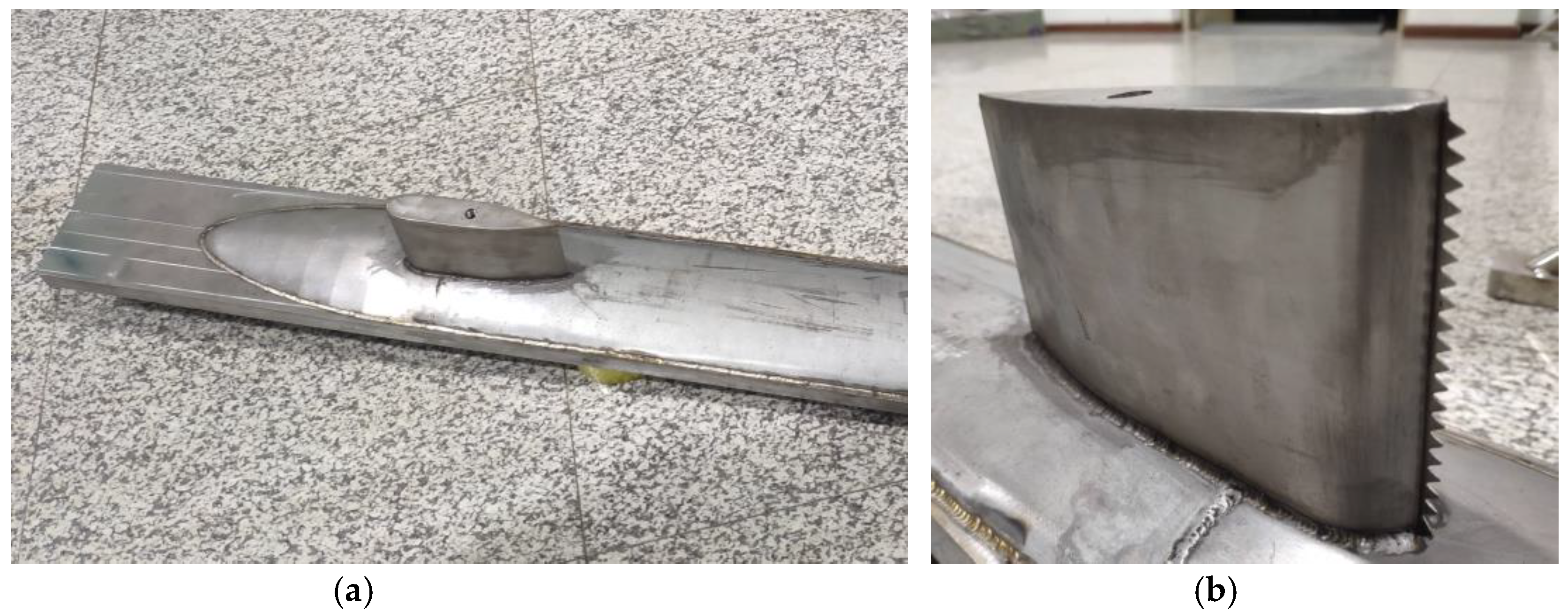
Figure 20 shows the picture of the original model and the model with leading-edge serrations. The parameters are as follows: the amplitude of the leading-edge serrations is 0.025c, and the wavelength of the leading-edge serrations is 0.05h, where c is the chord length and h is the height of the sail hull. The sound radiation power from the two models was measured by the reverberation method. Due to the measured frequency limitation of the reverberation tank, we put a fluctuation pressure sensor inside the sail hull to measure the turbulent fluctuation pressure instead of hydrophones, because the latter’s sensitivity is lower. Since the inside space of the sail hull is too small, we could place other fluctuation pressure sensors.
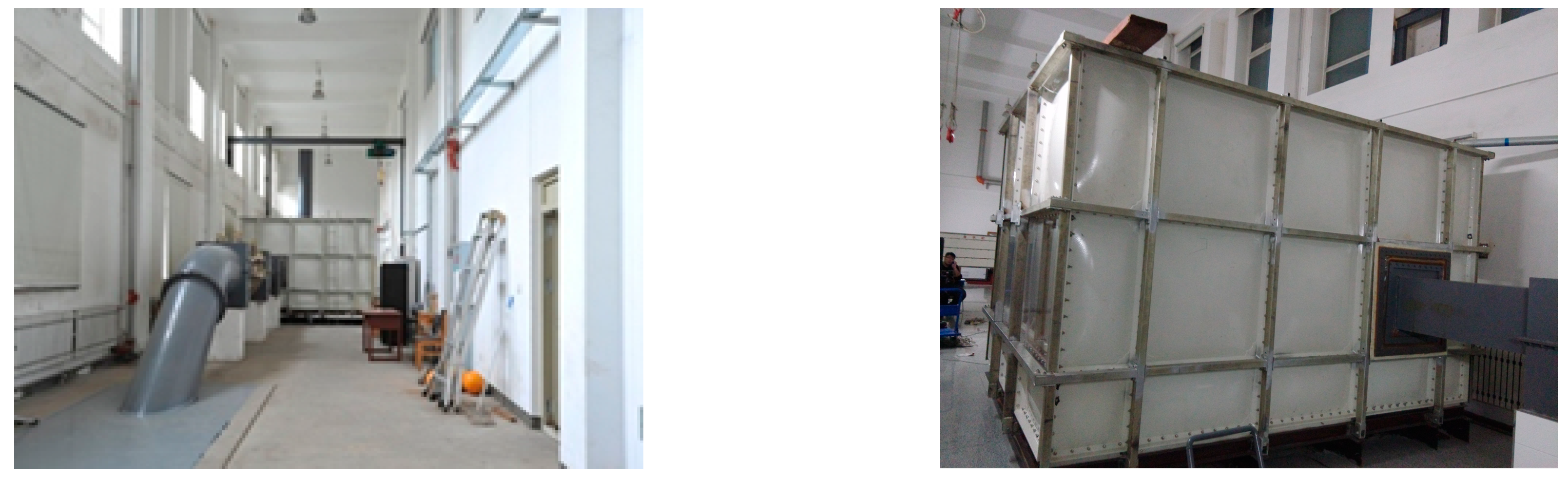
The gravity water tunnel is composed of a water tank, a contraction section, a rectifying section, a working section, a diffusion section, and the pipes. Each model was installed in the working section. To reduce the vibration from the other sections, an iron sand box and a Helmholtz muffler are installed at both ends of the working section.
Outside the working section, there is a reverberation tank made of steel and plastic, as shown in
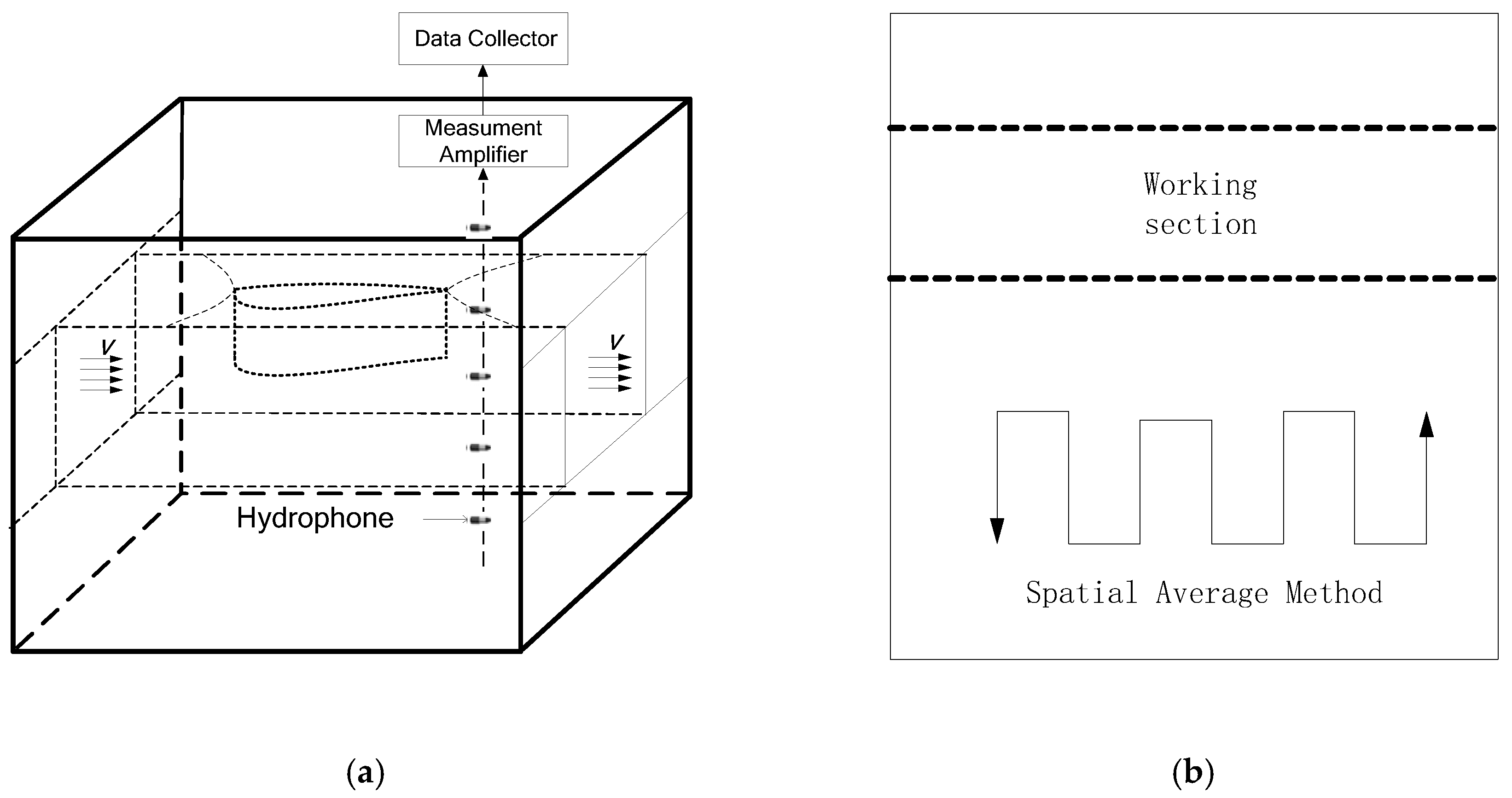
Figure 21. The bottom of the reverberation tank is vibration-damped to eliminate the vibration from the ground. In the reverberation tank, a vertical array of five hydrophones has been arranged in the reverberation area to measure the spatial average sound pressure, as shown in
Figure 22. The sound radiation power of the hydrodynamic noise was calculated according to Equation (30).
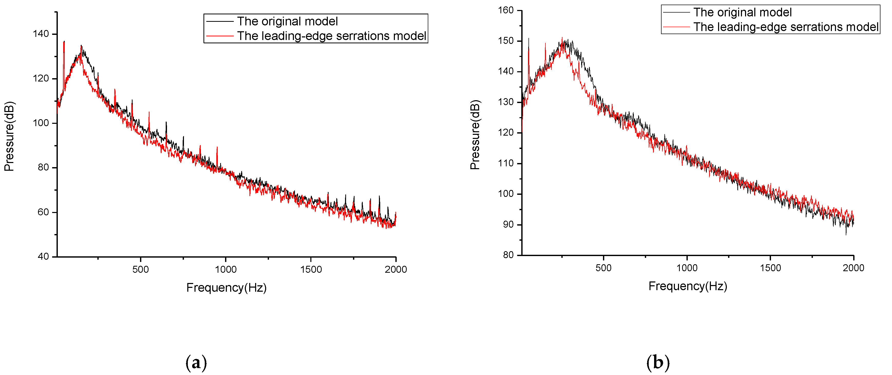
The measured frequency by the reverberation method in the reverberation tank was estimated as above 500 Hz. Below this frequency, we compared the sensitivities from the fluctuation pressure sensor and the hydrophone. Then, we calculated the sound pressure level using the data from the fluctuation pressure sensor. Since the space of the inside sail hull is small, the sound pressure collected by the fluctuation pressure sensor can be considered as spatial averaging. Therefore, we were able to calculate the total level of sound radiation power. The velocity of the water flow was 4.62 m/s and 8.68 m/s.
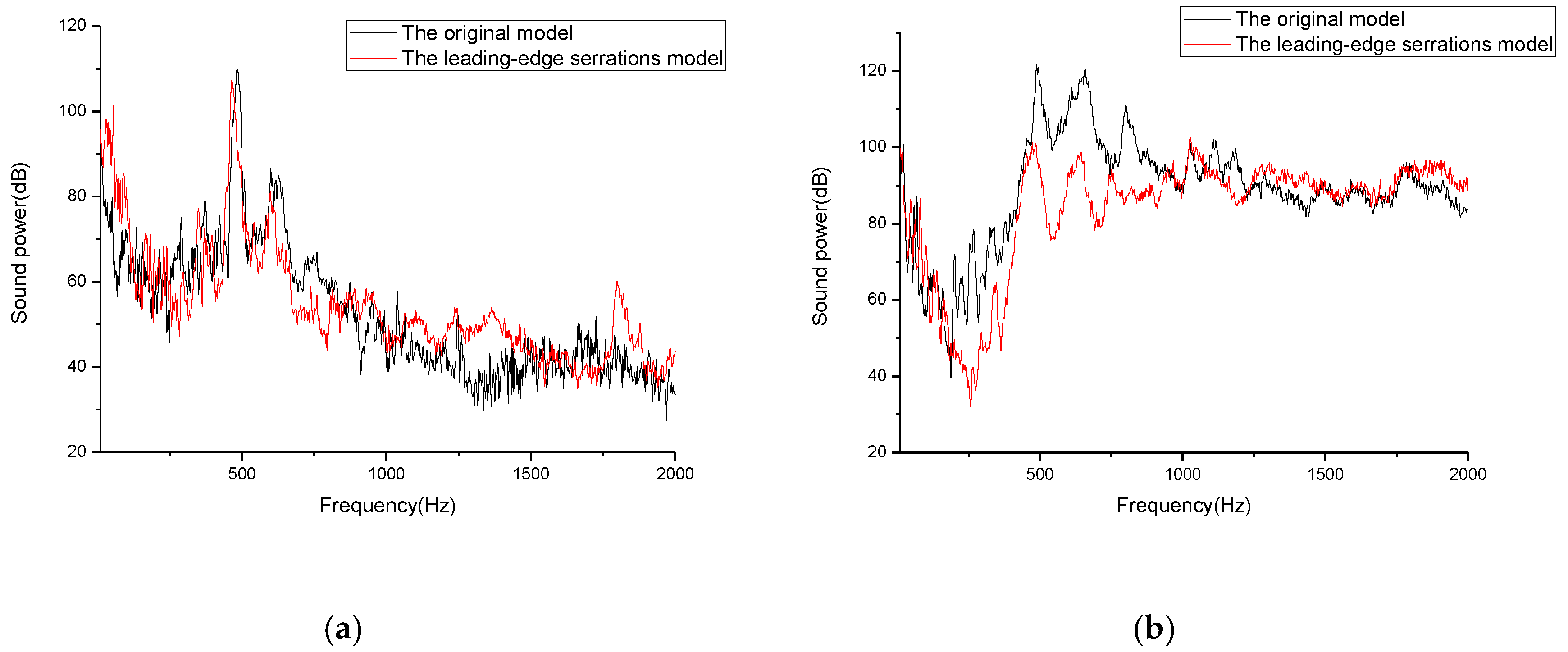
Figure 23 shows the turbulent fluctuation pressure collected by the fluctuation pressure sensor.
In
Figure 23, we can see that the turbulent fluctuation pressure has been suppressed in the low-frequency range, after the placement of leading-edge serrations. However, a high peak is observed at the frequency of 50 Hz. Through detailed analysis, the pressure level of this frequency was found to not have changed in the two experimental measurements: first, the measurement of the original model, and second, the measurement of the model with leading-edge serrations. We concluded that this peak frequency was generated from the electricity power supply. Since the fluctuation pressure sensor must be amplified by a conditioner, the conditioner can only work under an AC (Alternating Current) supply. In our country, the frequency of the electricity power supply is 50 Hz; therefore, the high peak at 50 Hz may come from the interference of the AC supply. In the data analysis, we have ignored this peak.
Compared with
Figure 19, we can see that the trend of the pressure changing with the frequency is very similar to
Figure 23b. If the frequency is less than 1000 Hz, the leading-edge serrations can suppress the hydrodynamic noise. When the frequency is higher than 1000 Hz, the leading-edge serrations can enhance the hydrodynamic noise.
Figure 24 shows the sound radiation power collected in the reverberation tank. We can see that when the frequency is less than 500 Hz, the sound radiation power from the two models is very low. This phenomenon clearly shows the measured frequency limitation, which is an intrinsic property of the reverberation tank.
If the frequency is less than 1000 Hz, the sound radiation power from the model with leading-edge serrations is less than that in the original model. When the frequency is higher than 1000 Hz, the sound radiation power from the model with leading-edge serrations is bigger than the original model. Therefore, the trend of sound radiation power changing with the frequency in
Figure 24b is similar to that in
Figure 19.
Through the statistical analysis, we found that the total sound radiation power of the two models is approximately proportional to the sixth power of the flow velocity. This phenomenon agrees well with the law of hydrodynamic noise. Due to time limitations, we have not calculated the noise reduction level of sound radiation power by leading-edge serrations at a flow velocity of 4.62 m/s. The measured total noise reduction level of sound radiation power by leading-edge serrations at a flow velocity of 4.62 m/s is 3.92 dB. The measured total noise reduction level of sound radiation power by leading-edge serrations is 8.89 dB at the flow velocity of 8.68 m/s. All of these results show that leading-edge serrations can be used to suppress hydrodynamic noise in scaled submarine models.
Through the comparison of the two models, the calculated noise reduction level of sound radiation power at a flow velocity of 8.68 m/s is 10.19 dB, as shown in
Table 4. However, there are still some differences between the numerical simulation and the experimental measurement.
First, the sail hull has been welded onto part of the submarine body. The experimental model is not as smooth as that in the numerical simulation.
Second, the thicknesses of the models in the numerical simulation are identical. However, the thicknesses of the models in the experiment are not identical, due to mechanical manufacturing limitations.
Third, there is no background noise in the numerical simulation. In the experiment, we could not entirely avoid the background noise from the ground, the circular pipes, the power supply, and so forth.
Fourth, other interferences also exist. For example, the flow velocity measurement repetition, the temperature of the water, and the boundary conditions in the experiment were not considered as rigid.
However, the measured level of hydrodynamic noise suppression is only 1.3 dB lower than the calculated level of hydrodynamic noise reduction. Since the models in the simulation and experiments are much smaller than real submarines, the noise reduction effect is obvious. We may conclude that if leading-edge serrations were to be placed on a larger model, the noise reduction level would be much more considerable. Therefore, we believe that the proposed noise reduction method by leading-edge serrations in our research can be applied to the enhancement of the acoustic stealth of underwater vehicles in the future.
7. Conclusions
Based on the results in the aerodynamic field, we placed leading-edge serrations onto the sail hull of a SUBOFF model to reduce its hydrodynamic noise. We investigated the flow field and the sound field of the original model with and without leading-edge serrations, by both numerical calculation and experiment testing. The flow field was calculated using the large-eddy simulation. The sound field was estimated by the wavenumber–frequency spectrum. The sound field was calculated by a combination of Lighthill’s acoustic analogy and the infinite element method. Since leading-edge serrations can break large-scale eddies into small-scale eddies, we focused on the suppression effect of the horseshoe vortex, because the horseshoe vortex is the main low-frequency noise source. The two significant parameters of leading-edge serrations—the amplitude and the wavelength—were comprehensively studied. To achieve the optimum noise reduction, we summarized the parameters of leading-edge serrations through the sound radiation power comparison between the original model and the model with leading-edge serrations of different amplitudes and different wavelengths. After that, we created two steel models according to the dimensions in the simulation. The experimental test was undertaken in a gravity water tunnel. Then, the calculated results were validated by the experimental measurement. The conclusions that we have reached are as follows:
First, leading-edge serrations can decrease the adverse pressure gradient of the sail hull. The formation of the horseshoe vortex is influenced by leading-edge serrations. Therefore, leading-edge serrations can be a feasible flow technique to suppress the flow-induced noise caused by the horseshoe vortex.
Second, leading-edge serrations can delay the boundary layer separation at the trailing edge of the sail hull. The flow-induced noise excited by the tail vortex shedding can be inhibited by leading-edge serrations.
Third, the amplitude of leading-edge serrations is a key parameter of the noise reduction. If the amplitude becomes shorter, better flow-induced noise reduction can be obtained. However, this parameter can only be achieved based on the evaluation effect of noise reduction.
Fourth, the wavelength of leading-edge serrations is another important parameter for noise reduction. If the wavelength becomes smaller, better flow-induced noise reduction can be achieved.
Fifth, an amplitude of 0.025c and a wavelength of 0.05h of the leading-edge serrations can achieve an optimum flow-induced noise reduction for the model in our study, where c is the chord length and h is the height of the sail hull.
Sixth, the noise reduction level of the experimental test is in good accordance with that of the numerical simulation. Therefore, the hydrodynamic noise reduction by leading-edge serrations has been validated.
Since our research model is scaled too much, yet the effect of noise reduction is greater than 6 dB, we may conclude that larger models could achieve a more obvious level of noise reduction, especially in the low-frequency range. We also believe that the results in this paper can provide some reference for the design of underwater vehicles with low hydrodynamic noise, such as submarines, torpedoes, and UUVs.


