Toward Realistic Ship Fuel Consumption Prediction Under Chronological Validation

Abstract

Accurate prediction of ship propulsion fuel consumption from operational data is important for performance assessment and energy efficiency management. This study examines how temporal structure and validation strategy influence the predictive performance of regression-based fuel consumption models using real operational data from a seagoing vessel. A controlled experimental framework is used to isolate the effects of chronological validation, temporal feature augmentation based on operational inputs, and autoregressive target information. Under strict chronological validation, a baseline regression model achieves R² = 0.788, while temporal feature augmentation improves performance to R² = 0.845 without using past fuel consumption values. An autoregressive configuration yields R² = 0.982, reflecting strong short-term persistence in the fuel consumption signal. Additional experiments show that random data partitioning can inflate reported R² by up to 0.19 compared with chronological evaluation. The results demonstrate that reported predictive accuracy depends strongly on evaluation design and temporal information structure, highlighting the importance of chronological validation for realistic operational prediction.

1. Introduction

Enhancing ship energy efficiency has become a critical issue for the maritime industry, primarily driven by the need to control operating costs and comply with increasingly stringent environmental regulations. The International Maritime Organization’s (IMO) 2022 Strategy on Reduction of GHG Emissions from Ships sets out ambitious decarbonization objectives, while amendments to MARPOL Annex VI introduce the Energy Efficiency Existing Ship Index (EEXI) and the Carbon Intensity Indicator (CII) as mandatory requirements for existing ships from 2023, thereby defining the current regulatory framework for operational energy efficiency [1,2,3].

Accurate prediction of ship propulsion fuel consumption is fundamental to achieving these goals, enabling optimized speed management, voyage planning, and trim optimization. Reliable estimation of fuel demand also contributes to operational safety, as significant errors in fuel consumption prediction may affect voyage planning and fuel reserve management, particularly on long passages or in regions where bunkering options are limited. While physics-based white-box models offer interpretability, they often struggle with the complexity and dynamic variability of real-world operations. This complexity arises from multifaceted factors including intricate hydrodynamic interactions [4], dynamic wind-assisted propulsion effects [5], and the need for real-time adaptation to changing meteorological conditions [6]; these are challenges that are difficult to fully encapsulate in analytical formulations.

Consequently, data-driven approaches, particularly machine learning (ML), have gained prominence for their ability to model complex, nonlinear relationships from high-frequency operational data. The field has evolved from foundational statistical models [7,8]; to sophisticated, integrated decision-support systems. Several studies have applied tree-based ensemble methods to ship fuel consumption prediction. These include Random Forest and gradient boosting approaches applied to operational vessel datasets, demonstrating the suitability of tabular machine learning models for capturing nonlinear relationships between operational and environmental variables [9,10,11], Bayesian-optimized systems for real-time fuel savings on ferries [12], and privacy-preserving fleet consumption models using federated learning [13]. Additionally, ML has proven effective for harbor vessel consumption prediction [14] and analysis of engine performance curves [15], demonstrating its versatility in maritime energy management.

Recent studies increasingly employ deep learning architectures to capture temporal dependencies in operational ship data. Typical approaches include recurrent neural networks and transformer-based sequence models that process sliding windows of historical observations [16,17,18]. These architectures learn temporal persistence in the fuel consumption signal through sequential input representations.

However, an important limitation of many recent deep learning approaches lies in their reliance on sliding temporal windows that include past fuel consumption values. While such autoregressive configurations are effective for short-term tracking and monitoring, they are less suitable for prospective operational scenarios in which future fuel consumption must be estimated without access to target history. In addition, increased architectural complexity may reduce interpretability and create practical challenges related to model validation, integration, and operational transparency in shipboard decision-support systems, where model transparency is essential for operational use [19].

These limitations indicate the need for modeling approaches that support forward prediction based solely on operational and environmental variables. Although feature engineering is widely recognized as a key component of data-driven modeling, temporal dependencies in fuel consumption studies are typically addressed through sequence architectures rather than through low-complexity temporal representations of input variables. This tight coupling between temporal learning and model complexity limits transparency and adaptability in operational environments.

The present study follows a different strategy by introducing time-aware feature engineering within a simple regression framework. Lagged values and rolling statistics of key operational and environmental parameters are used to represent short-term dynamics, while past fuel consumption is deliberately excluded. This enables the model to support genuine predictive and optimization applications where future fuel use is unknown.

The objective of this study is to assess whether temporal information derived solely from operational inputs improves predictive performance under realistic chronological conditions. By separating feature-level temporal representation from autoregressive persistence, the analysis isolates the contribution of operational dynamics to predictive capability without increasing model complexity.

Zhang et al. [20] developed a deep learning model based on BiLSTM for fuel consumption prediction using time-windowed operational data. The model processes sequential input data over fixed temporal horizons, enabling the network to capture temporal persistence and short-term dependencies present in the fuel consumption signal. Chen et al. [21] conducted a comparative study of several time-series deep learning architectures, including RNN, LSTM, Transformer, and Informer models. All evaluated configurations rely on sliding temporal windows of historical observations, where past fuel consumption values form part of the input sequence for predicting future states. Hu et al. [22] proposed an event-triggered Informer-based gray-box model for long-term fuel consumption prediction. The method operates on historical time-series sequences, exploiting temporal continuity in the system response through windowed input representations that include past fuel consumption behavior. Zhong et al. [18] proposed a hybrid architecture combining Residual Graph Convolutional Networks (ResGCN) with iLSTM and a multi-scale dynamic attention mechanism. The model is designed to capture both spatial relationships among ship operational parameters and complex temporal dependencies across multiple time scales. While this approach achieves high predictive accuracy, it relies on sequential input data that incorporate historical system states and therefore may primarily reflect temporal persistence rather than independent predictive relationships.

Beyond architectural complexity, reported predictive performance in ship fuel consumption studies is also strongly influenced by the information content of the input variables and the evaluation strategy. Previous work has shown that the predictive capability of tabular regression models in ship energy applications depends strongly on the physical relevance and information content of the selected inputs, highlighting the importance of domain-informed dataset analysis and feature selection [19].

Some recent studies include propulsion state variables such as engine load or shaft power among the predictors [23,24]. Since these quantities are physically coupled with fuel consumption and represent system-response variables rather than independent inputs available at decision time, their inclusion substantially increases the explained variance and reflects monitoring or nowcasting conditions rather than forward prediction capability. In addition, high accuracy has also been reported when temporally ordered operational data are randomly partitioned into training and test sets [10], which may lead to optimistic performance estimates due to temporal dependence between samples. From a methodological perspective, evaluation procedures that ignore temporal structure may violate key assumptions of time-series prediction [25].

Taken together, these observations indicate that differences in reported accuracy often reflect variations in temporal persistence, information availability, and validation design rather than model capability alone. However, these factors are typically addressed separately in the literature, which makes performance comparisons difficult and obscures the operational interpretation of reported results. This also explains why many published studies report very high predictive accuracy, as such results may reflect favorable evaluation conditions and information structure rather than true generalization to unseen future operating scenarios.

Within this context, the present study does not aim to introduce a new prediction architecture, but to examine how temporal structure and evaluation methodology influence the realism and interpretation of model performance. Numerous studies have already compared alternative machine learning algorithms for ship fuel consumption prediction. In contrast, the present study keeps the learning algorithm fixed in order to isolate the effects of temporal feature representation and evaluation strategy on reported predictive performance.

To address these methodological issues, this study proposes a controlled experimental framework that isolates the effects of (i) chronological validation, (ii) feature-level temporal information derived from operational and environmental variables, and (iii) short-term persistence introduced by autoregressive target inputs. By separating these factors under identical data and modeling conditions, the study enables a consistent and operationally meaningful interpretation of reported predictive performance. The main scientific contributions can be summarized as follows:

A controlled experimental framework that isolates the effects of chronological validation, input-based temporal information, and autoregressive persistence on reported model performance in ship fuel consumption prediction.

Quantification of the impact of evaluation strategy by directly comparing chronological and random data partitioning, demonstrating how temporal dependence can substantially inflate reported performance.

Systematic evaluation of feature-level temporal representation using lagged values and rolling statistics of operational and environmental variables within a low-complexity tabular regression framework.

Quantitative analysis of the performance gap between input-only temporal modeling and autoregressive configurations, clarifying the distinction between persistence-driven monitoring (nowcasting) and predictive modeling based on operational drivers.

Quantification of validation-induced performance inflation: the study shows that random data partitioning can increase the reported coefficient of determination by approximately 0.14–0.19 under identical data and model conditions, providing an empirically grounded reference for interpreting predictive performance in future studies.

2. Materials and Methods

2.1. Methodological Framework

This study addresses the problem of predicting ship energy efficiency using supervised regression models applied to operational and environmental data. The response variable represents propulsion fuel consumption, serving as a practical indicator of energy efficiency under varying operating conditions.

Unlike conventional regression approaches that treat observations as temporally independent, the proposed framework explicitly accounts for short-term temporal structure in the data. Rather than employing sequence-learning architectures, temporal dependency is incorporated at the feature level through lagged and rolling representations of selected input variables, a well-established approach in time-series analysis and machine learning for time series [26,27].

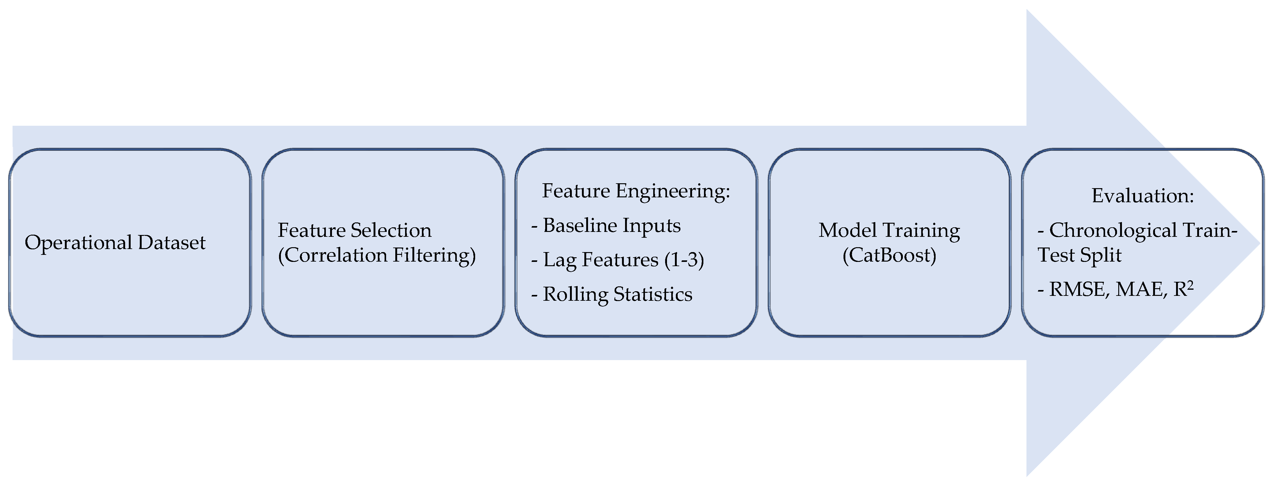
The overall methodological workflow of the study is illustrated in Figure 1.

This design enables controlled model complexity and preserves interpretability, while allowing short-term operational memory to be encoded within a stateless regression structure. The focus of the framework is therefore on assessing how explicit temporal feature augmentation influences regression performance under a controlled and reproducible modeling setup.

The methodological workflow consists of data preparation, feature engineering, model training, and performance evaluation. Model assessment is conducted using time-based train–test splits to reflect realistic operational deployment and to prevent information leakage, which can arise when standard cross-validation is applied to temporally ordered data [25]. Emphasis is placed on methodological transparency, reproducibility, and alignment with engineering interpretation, rather than on architectural complexity or purely accuracy-driven model design.

The analysis is based on the operational dataset previously published by Vorkapić et al. [9] and collected from a seagoing merchant vessel. The dataset integrates four primary sources: onboard automation system measurements, navigational data from ECDIS, operational records from noon reports, and external meteorological and oceanographic data corresponding to the vessel’s trajectory. The dataset is used without modification in order to ensure methodological consistency with the previous study and to isolate the effects of the revised modeling and evaluation approach introduced in the present work.

Within this framework, regression models designed for tabular data are employed, with CatBoost used as the primary learning algorithm [26,28], and the model configuration is kept consistent with the previous study to ensure a controlled comparison. Temporal dependencies are introduced at the feature level rather than through sequence modeling. Lagged values up to three previous observations (lags 1–3) and rolling statistics (mean and standard deviation over a window of three observations) are computed for selected operational and environmental variables. All temporal features are constructed using shifted windows to ensure strict temporal causality and to prevent information leakage.

The temporal features were applied to variables that represent dynamic operational and environmental conditions affecting propulsion power demand. These include propulsion state variables such as main engine RPM, vessel loading indicators such as draft and trim, and environmental factors including wind speed, wave height, and current conditions. Such variables are widely recognized in the literature as key drivers of ship fuel consumption due to their influence on propulsion load and hydrodynamic resistance.

A short window of three observations was used to capture immediate operational dynamics while limiting feature growth and reducing the risk of overfitting. Temporal augmentation was therefore restricted to physically relevant variables, with feature selection guided by engineering considerations and observed temporal continuity.

Lagged values of the target variable were excluded from the primary model to avoid autoregressive dependence and to preserve applicability to prospective prediction and optimization tasks. The learning algorithm and its configuration were kept fixed across all experiments to ensure that performance differences reflect the contribution of temporal input features rather than changes in model structure.

2.2. Data Source and Data Preparation

The initial candidate feature space comprised more than 100 onboard operational and environmental variables obtained from a continuous real-world operational dataset previously described in the Sensors study [9]. The dataset was collected from a seagoing liquefied petroleum gas (LPG) carrier with a capacity of 54,340 DWT, length of 225 m, and beam of 37 m. The vessel is equipped with a two-stroke HYUNDAI-MAN B&W 6G60ME-C9.2 main engine with a maximum output power of 12,400 kW and a fixed-pitch propeller (Hyundai Heavy Industries Co., Ltd., Ulsan, Republic of Korea). Among the available measurements, the variables most directly related to propulsion fuel demand represent dynamic operational and environmental conditions affecting propulsion power requirements. These include propulsion state variables such as main engine RPM, vessel loading indicators such as draft and trim, and environmental factors including wind speed, wave height, and current conditions.

The dataset covers the period from December 2016 to July 2017 and contains 18,499 time-ordered observations recorded from onboard monitoring systems at an approximately five-minute sampling interval. Non-operational conditions such as port stays, anchoring, drifting, berthing, and unberthing operations were excluded during preprocessing to focus on propulsion performance under normal navigation conditions. The selected data sources capture the principal factors influencing ship fuel consumption, including propulsion system operation, vessel loading condition, navigational state, and environmental resistance from wind, waves, and currents (

Table 1. Input and output variables in the prediction model.

No.	Variable	Unit	Source	Description
1	ME RPM	min−1	AMS	Main engine rotational speed
2	Air temperature	°C	AMS	Ambient air temperature
3	Sea water temperature	°C	AMS	Sea surface water temperature
4	Wind speed	knots	Anemometer	Measured wind speed
5	COG	°	ECDIS	Course over ground
6	Trim	m	AMS	Longitudinal inclination, positive aft
7	List	°	AMS	Transverse inclination
8	Wind direction	°	ECDIS	Wind direction relative to north
9	Uwind	m/s	Meteo-ocean data	Zonal wind component
10	Vwind	m/s	Meteo-ocean data	Meridional wind component
11	Draft_mean	m	AMS	Mean draft
12	Wind gust	m/s	Meteo-ocean data	Maximum short-term wind speed
13	Wave period	s	Meteo-ocean data	Dominant wave period
14	Sea state (logbook)	DSS	Ship’s logbook	Douglas Sea Scale
15	Significant wave height	m	Meteo-ocean data	Significant wave height
16	Sea current speed	m/s	Meteo-ocean data	Sea current magnitude
17	Wave direction	°	Meteo-ocean data	Direction of dominant waves
18	Sea direction	°	Meteo-ocean data	Direction of sea current
19	Swell (logbook)	DSS	Ship’s logbook	Douglas scale for swell
20	Wind (logbook)	Bft	Ship’s logbook	Beaufort wind scale
21	Propulsion fuel consumption	kg/h	AMS	Outlet variable

).

To control model complexity and preserve physical interpretability, domain-expert screening and correlation-based redundancy analysis were applied following the methodology established in that work. Pearson correlation analysis was used to identify highly correlated variables, and features with correlation coefficients exceeding 0.85 were removed unless they retained distinct physical relevance under transient or adverse operating conditions. The threshold of 0.85 was selected as a commonly used criterion for identifying strong linear dependence between predictors while preserving variables that may carry distinct operational meaning despite partial correlation. Removing highly correlated predictors reduces redundancy in the feature space and helps prevent multiple variables from representing the same physical information, which may otherwise bias the learning process or unnecessarily increase model complexity. This filtering step therefore improves the interpretability and stability of the regression model while preserving the most physically meaningful operational variables. To ensure methodological consistency and to isolate the effect of temporal feature representation, the same set of 20 input variables was retained unchanged in the present study, while propulsion fuel consumption was selected as the response variable. By keeping the feature set fixed and independent of the target variable, the analysis isolates the impact of temporal augmentation and evaluation strategy rather than improvements resulting from feature re-selection or target-driven optimization.

Derived efficiency indicators were excluded to prevent information leakage, while raw sensor signals were preserved. The dataset was obtained from the previously published study, where measurements from multiple onboard and environmental sources were temporally synchronized using a common timestamp and averaged where necessary. In the present study, the data were used in the processed form as provided, and no additional temporal resampling or interpolation was performed. Observations were treated as sequential records ordered in time, and lag features (1–3) represent short-term dependencies across consecutive observations.

The data were split chronologically using an 80% training and 20% testing ratio, corresponding to 14,799 training and 3700 testing samples. For model configurations incorporating lagged features, the first three observations were discarded due to temporal shifting, resulting in effective sample sizes of 14,796 training and 3697 testing samples.

The chronological split was applied within a continuous operational period, with the training and testing subsets representing comparable operating regimes. Descriptive analysis of key input variables indicated consistent value ranges across the two periods, suggesting no significant distribution shift between training and testing data.

2.3. Evaluation Metrics

Model performance is evaluated using a rigorous time-based train–test split to reflect realistic operational deployment and to prevent information leakage across temporal boundaries. The dataset is ordered chronologically, with the earlier portion used for training and the remaining portion reserved for testing. Randomized sampling and cross-validation techniques are deliberately avoided, as they would violate the temporal structure of the data and yield optimistically biased performance estimates.

Given the supervised regression setting with a continuous response variable, model accuracy is assessed using three complementary standard regression metrics:

Root Mean Square Error (RMSE) quantifies overall prediction error with greater sensitivity to larger deviations:

$$RMSE=\sqrt{{\displaystyle \frac{1}{n}}{\displaystyle \sum _{i=1}^n}{(p_i-a_i)}^2}.$$

(1)

where p_i denotes the predicted value, a_i is the actual value, and n the number of samples.

Mean Absolute Error (MAE) provides a robust measure of average prediction accuracy by equally weighting all deviations:

$$MAE={\displaystyle \frac{1}{n}}{\displaystyle \sum _{i=1}^n}\left|p_i-a_i\right|.$$

(2)

Coefficient of Determination (R²) indicates the proportion of variance in propulsion fuel consumption explained by the model:

$$R^2=1-{\displaystyle \frac{{\displaystyle {\sum }_{i=1}^n}{\left(a_i-p_i\right)}^2}{{\displaystyle {\sum }_{i=1}^n}{\left(a_i-\overline{a}\right)}^2}},$$

(3)

where $\overline{a}$ is the mean of the actual values.

Together, RMSE, MAE, and R² provide a balanced assessment of predictive accuracy, error magnitude, and goodness of fit, and are sufficient for comparing stateless and time-aware models within the scope of this study.

All data processing, model development, evaluation, and visualization were performed using open-source software. The analysis pipeline was implemented in Python (version 3.10) using standard scientific libraries for data handling and numerical analysis. Model training was carried out using CatBoost (version 1.2.8), while visualization was performed using standard Python plotting libraries.

Models were trained using CatBoost with default regression settings (iterations = 1000, depth = 6, learning_rate = 0.03, loss_function = RMSE). No hyperparameter optimization was performed, and the same parameter configuration was used for all model variants to ensure a controlled comparison across experimental conditions.

All experiments were executed on a standard workstation equipped with an Apple M1 processor and 8 GB RAM running macOS Tahoe 26.2 (Apple Inc., Cupertino, CA, USA), using identical computational settings throughout. The stochastic components of the algorithm were handled using the internal randomization procedures of the CatBoost framework. Due to the moderate dataset size and the use of a tabular gradient boosting model, the computational cost remained low. Training of individual model configurations required only a short execution time on a standard CPU environment without hardware acceleration.

3. Results

This section reports the predictive performance of the baseline, time-aware, and AR models. All configurations were evaluated under identical training and testing conditions to enable a controlled comparison of the impact of temporal feature augmentation.

3.1. Baseline Regression Performance (Stateless Model)

The baseline configuration follows the feature set and general modeling approach of the previous study [9], using the same input variables without temporal augmentation. However, all models in the present work were evaluated using a consistent chronological train–test split to ensure a fair comparison focused solely on the effect of temporal feature augmentation.

Model performance is evaluated on a time-based train–test split using RMSE, MAE, and R². When evaluated on the temporally held-out test set, the model achieves a coefficient of determination of R² = 0.788, with a corresponding RMSE of 161.55 kg/h and a mean absolute error (MAE) of 139.32 kg/h (

Table 2. Performance Comparison of Regression Models.

Model Configuration	Features	RMSE	MAE	R2
Baseline (Stateless)	26	161.55	139.32	0.788
Time-aware (lag + rolling)	68	138.4	123.76	0.845
Autoregressive (nowcasting)	75	47.31	39.25	0.982

).

In regression-based operational prediction problems, no universal threshold defines an “acceptable” R² value, as performance depends on the variability of the system and the available predictors. Therefore, the baseline model is used as a reference configuration, and subsequent models are evaluated comparatively to quantify the effect of temporal information.

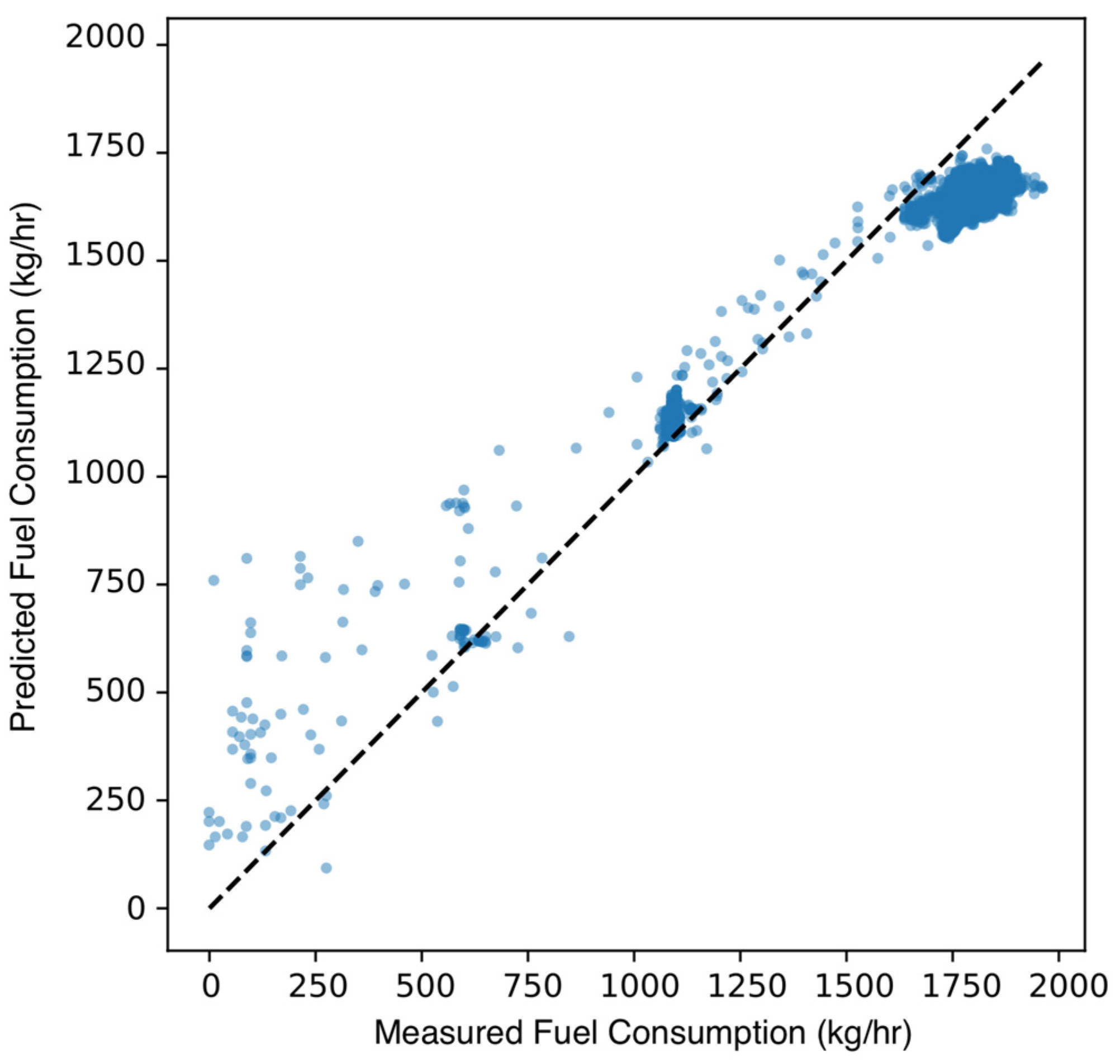
A scatter comparison between measured and predicted propulsion fuel consumption values for the baseline stateless regression model is shown in Figure 2, illustrating the overall agreement across the operating range.

While the scatter comparison confirms that the baseline model captures the dominant steady-state relationships, it does not provide insight into the model’s ability to track short-term dynamics.

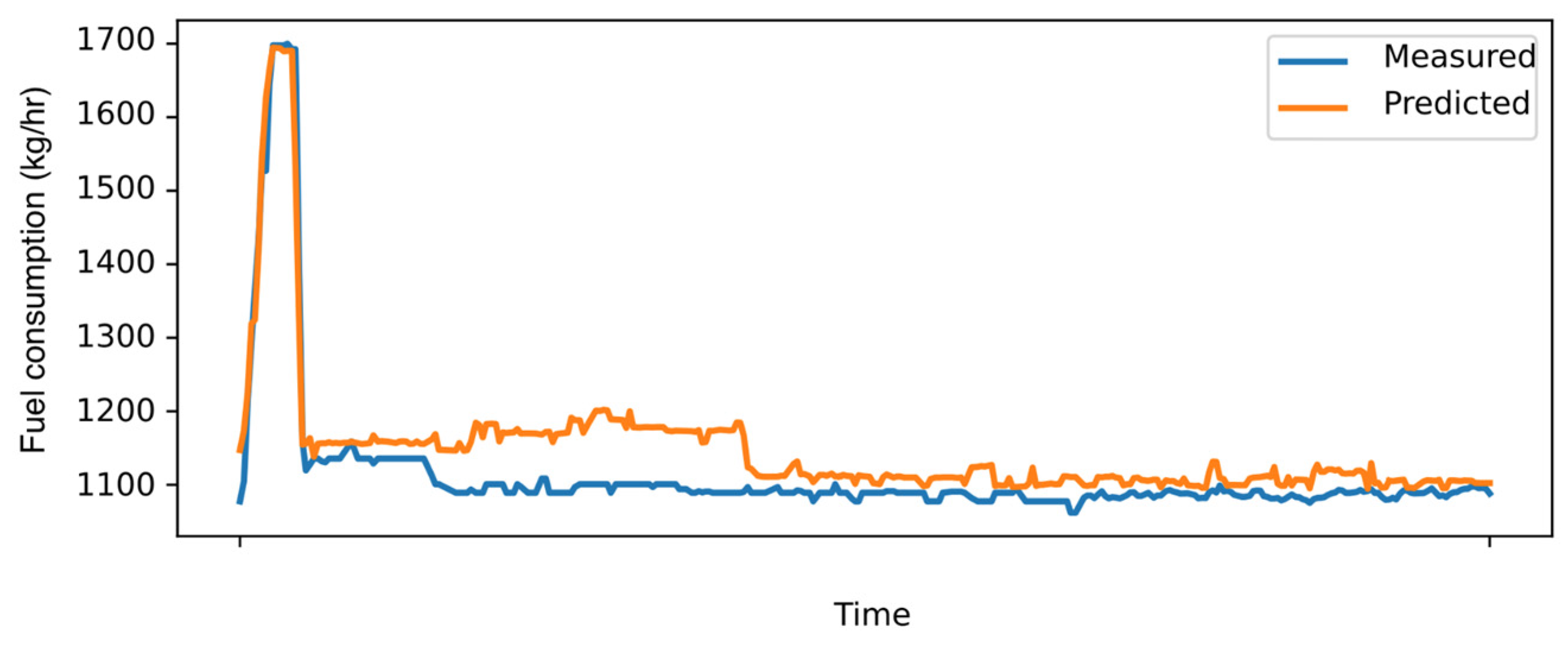
The figure illustrates a representative segment of the operational time series. Absolute timestamps are omitted from the horizontal axis for clarity; the axis represents the relative sequence of observations. The segment corresponds to a stable operating regime, whereas the complete dataset covers a wider range of engine loads and fuel consumption levels, as reflected in the scatter plot (Figure 2). The baseline model reproduces the global consumption trend but underrepresents short-term persistence and transient behavior. A representative time-series segment comparing measured and predicted propulsion fuel consumption for the baseline stateless regression model is shown in Figure 3. The baseline model reproduces general trends but exhibits limited ability to follow short-term persistence and transient variations, reflecting the absence of explicit temporal memory.

The baseline results establish a reference level of predictive accuracy against which the time-aware configuration is assessed. As expected, the stateless model captures the dominant steady-state relationships between propulsion fuel consumption and the selected operational and environmental inputs, but shows limited ability to represent short-term persistence and transient effects.

These baseline results provide a controlled benchmark for evaluating the contribution of explicit temporal feature engineering introduced in the subsequent analysis.

The corresponding performance metrics are summarized in Table 2.

The reported feature counts reflect both the primary input variables and additional derived features introduced during preprocessing. The baseline configuration consists of the 20 operational and environmental variables listed in Table 1, together with auxiliary time-context features derived from the timestamp, resulting in a total of 26 input features.

In the time-aware configuration, the feature space was expanded by applying lagged values (lags 1–3) and rolling statistics (mean and standard deviation over a three-observation window) to a subset of operational and environmental variables. This temporal augmentation added 42 derived features, increasing the total number of input features to 68.

The autoregressive (AR) configuration further included seven lagged values of the target variable, resulting in a total of 75 input features.

3.2. Time-Aware Model Performance

Introducing temporal information through lagged and rolling features of selected input variables leads to a consistent and measurable improvement in predictive performance. The time-aware regression model, which augments the baseline feature set with past values and rolling statistics of input variables only, achieves an R² = 0.845 on the same test set, with RMSE reduced to 138 kg/h and a corresponding reduction in MAE to 123.76 kg/h (Table 2).

The reported R² value should be interpreted in the context of strict chronological validation and the exclusion of autoregressive target information. Under these conditions, the model relies solely on operational and environmental predictors, and the resulting performance represents a realistic estimate of predictive capability for prospective operational deployment.

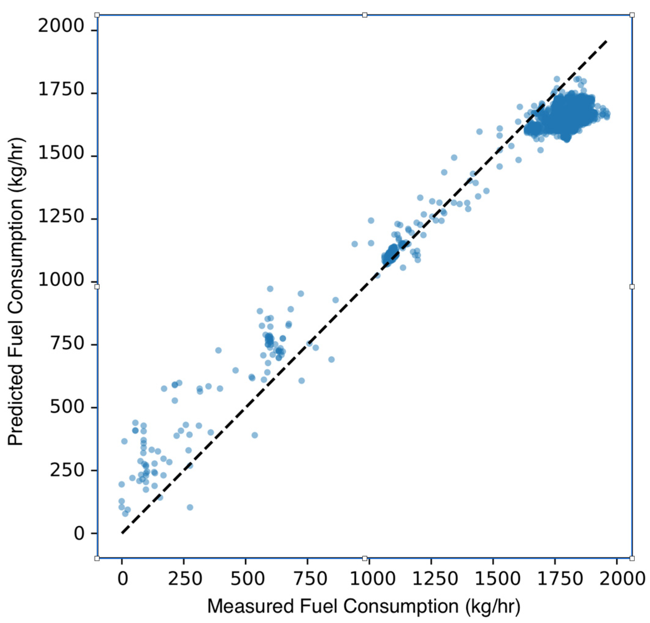
Compared to the stateless baseline, the time-aware model exhibits reduced dispersion around the one-to-one line, reflecting improved representation of short-term variability through explicit temporal feature augmentation. This improvement is illustrated in the measured versus predicted comparison shown in Figure 4.

Compared to the stateless baseline, the time-aware model demonstrates a consistent improvement across all evaluation metrics. The inclusion of short-term temporal context enables the regression model to better capture persistence effects and transient operating conditions that are not fully represented by instantaneous measurements alone. As a result, prediction errors are reduced and the overall goodness of fit is improved. Quantitative results reported in Table 2 confirm the observed improvement over the stateless baseline.

Importantly, these gains are achieved without increasing architectural complexity or introducing AR dependence on the target variable. The model remains a supervised tabular regression, with temporal information encoded explicitly at the feature level. This confirms that short-term temporal feature engineering can enhance predictive performance while maintaining transparency and controlled model behavior.

A direct comparison between the baseline and time-aware models highlights the impact of temporal feature engineering on predictive performance. Using the same input variables from the previous study and identical evaluation protocols, observed differences reflect temporal feature augmentation alone.

Across all reported metrics, the time-aware model consistently outperforms the baseline configuration. Reductions in RMSE and MAE indicate improved accuracy in capturing short-term variations in propulsion fuel consumption, while higher R² values reflect a better overall representation of variance in the response variable. These improvements are consistent with the presence of operational inertia and delayed system responses that cannot be fully described by instantaneous inputs alone.

The comparison confirms that introducing limited temporal memory at the feature level provides measurable benefits over a purely stateless regression approach. At the same time, the absence of additional sensors, architectural changes, or target autoregression ensures that the comparison remains controlled and methodologically transparent. As shown in Table 2, the time-aware configuration yields lower RMSE and MAE values and a higher R² compared to the baseline model.

3.3. Autoregressive Configuration for Short-Term Tracking

In addition to the stateless and time-aware models, a separate autoregressive (AR) configuration was evaluated to assess the effect of including past values of the target variable. In this setup, historical fuel consumption values were provided as inputs, allowing the model to exploit short-term temporal continuity in the response signal. The AR model achieved a coefficient of determination of R² = 0.982, with RMSE of 47 kg/h and MAE of 39.25 kg/h (Table 2).

The substantially higher accuracy reflects the strong short-term persistence present in the fuel consumption signal. However, this configuration depends on the availability of past target values and therefore differs in scope from models intended for prospective prediction based solely on operational and environmental inputs.

Accordingly, the AR model is considered a reference for short-term tracking performance rather than a candidate for operational energy efficiency prediction within the framework of this study.

3.4. Effect of Random vs. Chronological Evaluation

To assess the impact of evaluation methodology on reported performance, additional experiments were conducted using random train–test partitioning of the same dataset. All model configurations and hyperparameters were kept identical, allowing a controlled comparison between random and chronological evaluation.

Table 3. Validation-Induced Performance Differences: Chronological vs. Random Splitting.

Model	Chronological R2	Random R2	ΔR2
Baseline (Stateless)	0.788	0.978	+0.190
Time-aware (lag + rolling)	0.845	0.984	+0.139
Autoregressive (nowcasting)	0.982	0.992	+0.010

summarizes the resulting performance differences.

The results in Table 3 show that the data partitioning strategy has a pronounced effect on the reported predictive performance. When random train–test splitting is applied, the coefficient of determination increases substantially for models based solely on operational and environmental inputs. For the stateless baseline model, R² increases from 0.788 to 0.978 (ΔR² = +0.190), while the time-aware configuration increases from 0.845 to 0.984 (ΔR² = +0.139).

In contrast, the autoregressive configuration shows only a minor change in performance (ΔR² = +0.010). Because this model explicitly incorporates past fuel consumption, its predictive accuracy is already dominated by short-term temporal persistence and is therefore less sensitive to the partitioning strategy.

The large performance gains observed for the input-only models indicate that random partitioning allows strong temporal dependence and operating-regime similarity between training and test samples. Under such conditions, the evaluation may partially reflect temporal continuity within the dataset rather than the model’s ability to generalize to unseen future operating conditions.

These results demonstrate that evaluation methodology alone can increase reported R² by up to approximately 0.14–0.19. This finding highlights the importance of strict chronological validation when the objective is forward operational prediction and indicates that performance values obtained under random partitioning are not directly comparable to those derived under realistic chronological conditions.

Taken together, the results confirm that the observed differences in predictive accuracy arise primarily from evaluation design rather than from model capability. Importantly, these performance changes are obtained under identical data, feature sets, and model configurations, with the validation strategy as the only varying factor. This controlled comparison shows that evaluation design alone can inflate the reported coefficient of determination by approximately 0.14–0.19 in time-ordered maritime operational data, providing a quantitative reference for interpreting high predictive accuracies reported in the literature.

4. Discussion

The results show that incorporating temporal structure from operational inputs leads to a measurable improvement in fuel consumption prediction accuracy. The time-aware model increases the coefficient of determination from R² = 0.788 to R² = 0.845, with corresponding reductions in RMSE and MAE. This indicates that short-term operational history contains predictive information beyond instantaneous measurements. The moderate magnitude of the improvement suggests that the baseline model already captures the dominant steady-state relationships, while temporal features primarily represent transient behavior and system inertia.

Importantly, this improvement is achieved without using lagged values of the target variable. The model therefore remains suitable for prospective prediction and operational optimization scenarios where future fuel consumption must be estimated solely from operational and environmental conditions.

The substantially higher performance of the autoregressive configuration (R² = 0.982) reflects strong short-term persistence in the fuel consumption signal. While this property can be effectively exploited for short-horizon tracking and monitoring, it primarily represents persistence-driven accuracy rather than improved prediction based on operating conditions. Evaluating the autoregressive model separately therefore helps distinguish monitoring capability from predictive performance relevant for decision support. High predictive accuracies reported in recent ship fuel consumption studies are therefore not always directly comparable, as they depend strongly on the available input information and the evaluation strategy. In particular, performance may increase when models exploit temporal persistence, system-response variables that embed operational effects, or data partitioning approaches that do not fully preserve chronological structure. These findings indicate that part of the very high accuracy reported in the literature may reflect evaluation design and temporal information structure rather than genuine predictive capability under forward operational conditions.

In the earlier Sensors study, the model was also based exclusively on operational and environmental inputs, without the use of autoregressive target information or propulsion state proxies. However, the evaluation setting did not explicitly enforce strict chronological separation, which may allow regime similarity between training and test data. Together with the near-perfect performance observed for the autoregressive configuration in the present study, this indicates that very high R² values may reflect persistence effects or regime similarity rather than intrinsic model capability.

In contrast, the present input-only model, evaluated under strict chronological validation and using only decision-time operational and environmental variables, provides a more realistic estimate of predictive performance for forward operational deployment.

Additionally, a supplementary experiment comparing random and chronological data partitioning confirmed the sensitivity of reported performance to the validation strategy. When random splitting was applied to the same dataset, the baseline and time-aware configurations achieved R² values of 0.978 and 0.984, respectively, compared to 0.788 and 0.845 under chronological evaluation. This substantial increase (ΔR² ≈ +0.139 to +0.190) indicates that temporal dependence between training and test samples can lead to strongly optimistic performance estimates if chronological structure is not preserved.

From a physical perspective, the benefit of temporal input features is consistent with the dynamic response of ship propulsion systems. Fuel consumption depends not only on instantaneous operating conditions but also on recent load history, maneuvering activity, and delayed thermal and hydrodynamic effects. Encoding short-term temporal context at the feature level allows these transient effects to be captured without introducing explicit physical modeling or autoregressive dependence on the response variable.

Because these dynamics are most pronounced during changing operating conditions, the practical value of temporal augmentation is greatest in non-stationary regimes. During stable operation, the baseline model already captures the dominant steady-state relationships. This suggests that onboard implementations could adopt a mode-aware strategy, using simple stateless predictions under steady conditions and activating time-aware features when significant load or environmental changes are detected. In addition, the strong performance of the input-only configuration supports the use of models based on a limited set of physically meaningful variables, improving robustness, reducing sensor availability requirements, and simplifying maintenance in shipboard decision-support systems.

The moderate magnitude of the improvement further suggests that additional gains are more likely to depend on data quality, measurement accuracy, and the inclusion of additional operational or environmental information than on increased model complexity.

The analysis is based on data from a single vessel and operating profile. Although the observed behavior is consistent with known propulsion system characteristics, quantitative results may vary across different ship types and operating conditions. Extending the analysis to multiple vessels and longer operational periods represents an important direction for future work.

The results of this study should be interpreted in the context of strict chronological validation, which reflects realistic operational deployment conditions. Under this evaluation framework, the time-aware model demonstrates measurable improvement over the baseline while remaining applicable to prospective prediction scenarios. The separation of input-based temporal features from autoregressive configurations clarifies the contribution of operational dynamics versus short-term persistence, providing a transparent basis for model selection based on intended application scope.

The proposed modeling framework is designed with practical shipboard deployment in mind. Because the model relies exclusively on operational and environmental inputs that are routinely available from onboard monitoring systems, it can be integrated into existing vessel performance monitoring platforms without requiring additional sensors or complex data pipelines.

One potential application is real-time operational decision support. By estimating expected propulsion fuel consumption under given operating conditions, the model could assist officers and technical managers in evaluating speed adjustments, trim optimization strategies, or routing decisions. The time-aware configuration, which incorporates short-term temporal context from operational variables, can also improve the model’s ability to capture transient responses during changing environmental or operating conditions.

Another relevant application is performance monitoring and anomaly detection. Deviations between predicted and observed fuel consumption may indicate changes in hull condition, propulsion efficiency, or environmental disturbances, providing an additional diagnostic indicator for technical management and energy efficiency analysis.

Due to the relatively low computational cost and reliance on standard operational data, the proposed approach is suitable for deployment in onboard decision-support systems or fleet performance monitoring platforms.

5. Conclusions

This study examined how temporal structure and evaluation strategy affect the realism and operational interpretation of machine learning models for ship propulsion fuel consumption. Using the same operational dataset and baseline modeling framework as in previous work, a controlled analysis was conducted to isolate the effects of chronological validation, feature-level temporal augmentation, and autoregressive target information.

Incorporating short-term temporal context from operational and environmental inputs improved performance under strict chronological evaluation, increasing the coefficient of determination from R² = 0.788 to R² = 0.845. Because past fuel consumption was excluded, the resulting model remains suitable for prospective prediction and optimization based solely on available operating conditions.

The much higher accuracy obtained with the autoregressive configuration reflects strong short-term persistence in the fuel consumption signal. While effective for short-horizon tracking, such models rely on target history and therefore represent monitoring capability rather than forward prediction based on operational drivers. Evaluating this configuration separately allows persistence effects to be distinguished from physically meaningful predictive relationships.

The results indicate that, under realistic chronological conditions, performance improvements obtained from input-based temporal information represent genuine predictive capability, while very high accuracy values may primarily reflect temporal persistence, regime similarity, or additional information content rather than intrinsic model capability. A supplementary comparison between random and chronological data partitioning showed that random splitting increased the coefficient of determination by approximately 0.14–0.19 across model configurations, confirming that neglecting temporal structure can lead to substantially optimistic performance estimates. These findings support the use of chronological evaluation when benchmarking machine learning models intended for forward operational prediction.

Further improvements are likely to depend more on data quality, measurement accuracy, and the availability of operational and environmental information than on increased model complexity.

The analysis is based on operational data collected from a single seagoing LPG carrier, which means that the quantitative results reflect the specific operational characteristics of that vessel. Consequently, the reported predictive performance should not be directly generalized to other ship types or operating profiles. However, the methodological framework proposed in this study, including temporal feature engineering and chronological validation, is not vessel-specific and can be applied to other ships provided that comparable operational datasets are available.