Spatiotemporal Characteristics and Physical–Ecological Coupling Mechanisms of Spring Phytoplankton Blooms in the Bohai Sea

Abstract

Spring phytoplankton bloom mechanisms in the Bohai Sea show clear spatial differences, but the physical–biological coupling in the ice-covered Liaodong Bay (LDB) remains poorly understood. Utilizing satellite observations and high-resolution reanalysis data from 2009 to 2023, this study explores the drivers of spring blooms through generalized additive models (GAMs) and the Equation of State of Seawater (EOS). The results reveal pronounced regional heterogeneity. In the southern Bohai Sea, bloom dynamics are co-regulated by a complex combination of nutrient availability and localized physical mixing. In contrast, blooms in LDB are predominantly driven by the shoaling of the mixed layer depth (MLD), a physical state intrinsically linked to winter sea-ice melt. Linear decomposition of water density via EOS quantitatively demonstrates that spring stratification in LDB is salinity-dominated (contributing ~60.7%), rather than thermally driven. The rapid influx of low-salinity meltwater forms a strong halocline that suppresses vertical mixing and physically compresses the MLD into the euphotic zone. Consistent with Sverdrup’s Critical Depth Theory, this inferred physical pathway effectively alleviates light limitation and acts as the primary trigger for the early bloom peak timing. This complete melting–freshening–stratification–light coupling chain provides a novel physical perspective on how mid-latitude marginal sea ecosystems respond to climate change, distinct from canonical polar light-limitation models.

1. Introduction

Phytoplankton blooms, characterized by the rapid accumulation of algal biomass [1], are critical biological events in mid-to-high latitude shelf seas that regulate primary productivity and shape marine food web dynamics [2,3]. As China’s only semi-enclosed internal sea, the Bohai Sea (BS) is subject to intense human activity and terrigenous inputs, resulting in severe ecological stress and frequent eutrophication-driven blooms [4,5,6]. However, the mechanisms triggering these spring blooms exhibit pronounced spatial heterogeneity, largely due to distinct regional physical environments [7]. Notably, the BS is the lowest-latitude seasonal ice-covered sea in the Northern Hemisphere [8,9]. This unique physical setting suggests that bloom dynamics in the ice-covered LDB may diverge fundamentally from those in predominantly ice-free waters. While previous studies utilizing long-term satellite observations have characterized the spatiotemporal variations in chlorophyll-a in the BS [10], they have primarily focused on surface-based correlations with conventional environmental drivers such as wind fields, river discharge, and sea surface temperature (SST) [11,12]. As a result, the mechanistic linkage between winter sea-ice processes, stratification development, and subsequent bloom phenology has not been comprehensively explored. In particular, few studies have examined the interannual variability of bloom timing in relation to objectively defined ice-melt transitions and density-based stratification changes. A more integrated, process-oriented analysis is therefore needed to clarify how winter sea ice influences spring bloom dynamics in LDB.

In traditional high-latitude studies, sea ice is generally viewed as a barrier to photosynthetically active radiation (PAR), meaning blooms typically initiate only at the ice edge or following complete ice retreat due to under-ice light limitation [5,13,14]. However, Sverdrup’s Critical Depth Hypothesis posits that bloom initiation fundamentally requires the mixed layer depth (MLD) to shoal above a critical depth, a state where phytoplankton photosynthesis exceeds respiration [15]. In ice-affected waters, the release of freshwater during sea-ice melt provides a potent physical mechanism for this shoaling; the resulting low-salinity surface layer establishes a strong halocline that suppresses vertical turbulent mixing. This freshwater-induced stratification effectively compresses the MLD into the well-illuminated euphotic zone, thereby relieving light limitation and triggering spring blooms [16,17,18]. While Sverdrup’s framework emphasizes the balance between mixed layer depth and critical depth, the present study does not explicitly compute critical depth. Instead, we focus on diagnosing mixed layer depth variability and density-driven stratification changes as practical indicators of the transition from deep winter mixing to bloom-favorable conditions.

In shallow shelf environments, such as the BS, where bathymetry is limited and light levels increase rapidly in spring, the shoaling of the mixed layer provides a more direct and operational metric for assessing bloom initiation dynamics. Although this meltwater–stratification–bloom framework is well-documented in polar regions, its applicability to shallow, mid-latitude marginal seas remains uncertain. Unlike polar oceans, the BS is characterized by higher background solar radiation, shallow bathymetry, strong tidal mixing, and eutrophic conditions. Under such settings, it is crucial to determine whether sea-ice melt retains a dominant physical role or if thermal forcing and nutrient availability dictate bloom dynamics. Addressing this knowledge gap is the primary objective of this study.

To extend Sverdrup’s critical depth theory to seasonally ice-covered, mid-latitude systems, we propose a conceptual scheme built upon three interrelated hypotheses.

Hypothesis 1.

In the ice-dominated LDB, spring stratification is primarily driven by meltwater-induced surface freshening rather than the canonical mid-latitude mechanism of thermal surface warming.

Hypothesis 2.

Bloom drivers exhibit a spatial dichotomy; LDB dynamics are governed predominantly by physical controls, whereas biochemical factors dominate the largely ice-free southern BS.

Hypothesis 3.

The rapid influx of low-salinity meltwater functions as a critical physical switch, suppressing vertical mixing and compressing the MLD into the euphotic zone to trigger spring blooms in ice-affected mid-latitude bays.

By testing these hypotheses using satellite observations and high-resolution reanalysis data from 2009 to 2023, this study utilizes a combined generalized additive model (GAM) and density decomposition framework to explicitly isolate the physical effects of sea-ice melt. Ultimately, this work establishes an integrated meltwater–freshening–stratification–light conceptual scheme, offering novel physical insights into how mid-latitude marginal sea ecosystems respond to climate change.

2. Materials and Methods

2.1. Study Area

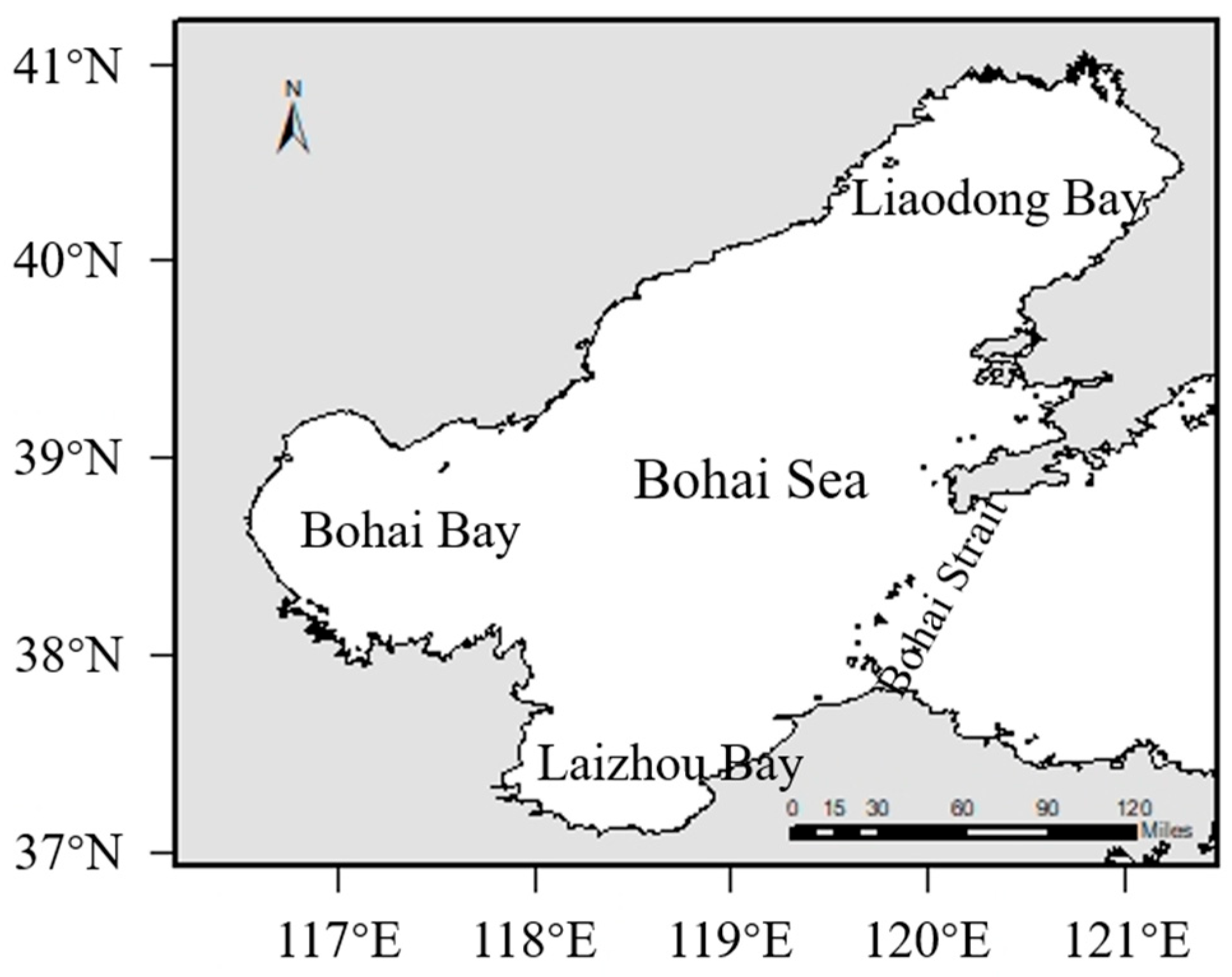
The study area covers the entire Bohai Sea (BS) (37° N–41° N, 117° E–122° E), a semi-enclosed shallow shelf sea with an average depth of only ~18 m [19]. Water exchange with the Yellow Sea is limited, occurring exclusively through the eastern Bohai Strait. Influenced by both the East Asian monsoon and terrigenous inputs, the thermohaline structure of the BS exhibits significant seasonal variability. Furthermore, high eutrophication levels provide a sufficient material basis for phytoplankton outbreaks [20]. Based on geographic features and hydrodynamic conditions, the BS is generally divided into three major bays—LDB in the north, Bohai Bay in the west, and Laizhou Bay in the south—along with the Central Bohai Basin (Figure 1).

2.2. Satellite Remote Sensing and Reanalysis Data

Chlorophyll-a (Chl-a) data were derived from the MODIS-Aqua Level 3 products in 2009–2023 (https://oceandata.sci.gsfc.nasa.gov/ (accessed on 2 May 2025)), with a temporal resolution of 8 days and a spatial resolution of 4 km. These products were retrieved using the OC3M ocean color algorithm. After spatial subsetting, regional Chl-a time series were generated by calculating the spatial arithmetic mean of all valid (cloud-free and ice-free) pixels within each predefined bay. The 8-day compositing of the Level-3 products naturally minimized daily data gaps; any remaining missing pixels within a region were excluded from the spatial average to avoid interpolation artifacts. From this robust regional time series, a spring (March–May) dataset was constructed to extract key ecological indices, including bloom intensity and initiation timing. For each subregion, spatial averaging yielded one representative annual value per variable, which was subsequently used for interannual statistical analysis (2009–2023, n = 15). Individual grid cells were not treated as independent samples in the modeling framework.

Winter sea-ice data were obtained from the daily snow and ice products of the Interactive Multisensor Snow and Ice Mapping System (IMS) provided by the National Snow and Ice Data Center (NSIDC) (https://nsidc.org/data/g02156/versions/1 (accessed on 2 May 2025)). The dataset features a spatial resolution of 4 km. The study period covers the winters from 2009 to 2023 (defined as December 1 to March 31 of the following year). Since the raw IMS data utilize a Polar Stereographic Projection, they were reprojected to the geographic coordinate system (WGS84) using the Mapping Toolbox, followed by a geometric correction of the latitude–longitude grids.

To quantitatively characterize the evolution of water column physical structures during sea-ice melting, Global Physical Reanalysis data (2009–2023) provided by the Copernicus Marine Environment Monitoring Service (CMEMS) (https://data.marine.copernicus.eu/products (accessed on 2 May 2025)) were utilized at a spatial resolution of 1/12°. This dataset provides high-resolution daily parameters for seawater potential temperature and sea surface salinity. To investigate the driving effects of physical processes on biogeochemical cycles, CMEMS Global Biogeochemical Reanalysis products (0.25° resolution) were synchronously employed to extract surface data for nitrate, phosphate, and silicate. It should be noted that the CMEMS biogeochemical reanalysis has a spatial resolution of 0.25°, which may limit its ability to accurately resolve fine-scale nutrient gradients in shallow estuarine and nearshore environments such as the Bohai Sea. Therefore, nutrient-related results in this study should be interpreted as indicative of regional-scale tendencies rather than precise nearshore concentrations. Consistent with this regional focus, we avoided pixel-by-pixel interpolation between the 4 km satellite data and the 0.25° biogeochemical grids. Direct spatial interpolation can introduce significant artificial errors in these complex coastal waters. Instead, all variables were independently averaged into regional means, which were then used directly as inputs for the generalized additive models (GAMs).

2.3. Data Processing and Statistical Methods

2.3.1. Calculation of Spring Bloom Intensity

To quantitatively characterize the intensity and phenological variability of spring phytoplankton blooms, this study adopts the maximum chlorophyll-a approach established by Park et al. [21] for assessing ice-driven spring blooms in marginal seas. For each pixel (i,j), the maximum chlorophyll-a concentration during the spring period (March–May) was first identified and used as an indicator of spring bloom intensity, which is expressed as

$$Chl{a}_{\max }\left(i,j\right)=\max \left[Chl{a}_3\left(i,j\right),Chl{a}_4\left(i,j\right),Chl{a}_5\left(i,j\right)\right]$$

(1)

The specific day on which this maximum chlorophyll-a concentration occurred was recorded as the bloom peak day of year (Bloom DOY), serving as the temporal metric to describe the timing of the spring bloom peak. This method effectively captures the spatial variability in bloom phenology, particularly in regions characterized by pronounced spatial heterogeneity.

Despite the widespread application of advanced phenological algorithms, such as threshold-based and derivative methods in long-term open ocean studies [22], their use in the Bohai Sea presents significant challenges. Threshold methods rely on a stable winter background baseline, which is highly susceptible to disruption in the Bohai Sea due to elevated turbidity from intense sediment resuspension in early spring. Previous research on optically complex coastal waters has indicated that interference from suspended particulate matter and colored dissolved organic matter (CDOM) can substantially increase the uncertainty associated with simple threshold-based approaches [23]. Derivative methods, in contrast, are highly sensitive to missing data points common in satellite observations, particularly in cloud-prone and ice-covered waters. Related studies have demonstrated that data gaps in time series can amplify noise and the risk of misclassification in derivative-based phenological metrics [24]. Therefore, effectively determining the maximum value can cut through high-frequency optical noise and reliably capture the spatiotemporal differences in bloom timing associated with meltwater-induced stratification events.

2.3.2. Calculation of Sea-Ice Parameters

Sea-ice area (SIA) was calculated using the IMS sea-ice product released by NOAA/NSIDC. Specifically, grid cells with a pixel value of 3 in the IMS dataset were classified as sea-ice-covered. The daily sea-ice area can be expressed as

$$S_{\mathrm{day}}=\sum _{i=1}^N\left({\delta }_i\times A_{\mathrm{cell}}\right)$$

(2)

where N denotes the total number of grid cells within the study region, ${\delta }_i$ is the sea-ice indicator for the i-th grid cell (equal to 1 when the pixel value is 3 and 0 otherwise), and A_cell represents the area of a single grid cell (approximately 16 km²). Based on the daily SIA, the annual mean and annual maximum sea-ice areas were further calculated to characterize interannual variability in sea-ice conditions.

The sea-ice melt date was defined as the first day, starting from 1 February of each year, when the regional sea-ice area decreased to zero and remained at zero for at least 15 consecutive days. The February 1st start date was selected to bypass the primary winter growth phase, as the peak ice season typically occurs in January or February. Furthermore, because the Bohai Sea is characterized by a pulsed, short-duration sea-ice regime prone to transient refreezing, the 15-day persistence window was implemented to filter out short-term synoptic weather fluctuations, ensuring the identified date represented the permanent seasonal retreat of sea ice. The melt date was expressed as the day of year (DOY), following the definition of Brown et al. [25].

2.3.3. Physical Environmental Parameters

The mixed layer depth (MLD) was determined using a density threshold criterion, defined as the shallowest depth at which the in situ seawater density ρ(z) differs from a reference density ρ_ref by a prescribed threshold

$$\rho \left(z\right)-{\rho }_{\mathrm{ref}}\ge {\displaystyle \frac{0.03 \mathrm{k}\mathrm{g}}{{\mathrm{m}}^3}}$$

(3)

where ρ_ref denotes the in situ density at the reference depth, and the shallowest depth satisfying this condition was taken as the MLD. The threshold value follows de Boyer Montégut et al. [26] and has been shown to effectively capture variations in upper-ocean mixing intensity. A shallower mixed layer indicates stronger stratification, which is generally favorable for the development of spring phytoplankton blooms

To quantitatively distinguish the relative contributions of temperature and salinity to spring water-column stratification, a linear decomposition of the density difference (Δρ) between the surface and bottom layers was performed based on the seawater equation of state. Under a given pressure, seawater density can be expressed as ρ = ρ (T, S). Considering that vertical gradients of temperature and salinity are relatively small during the spring ice-melt period, the density response to temperature and salinity variations can be approximated by a first-order linear relationship

$$\Delta \rho \approx {\left({\displaystyle \frac{\mathsf{\partial }\rho }{\mathsf{\partial }T}}\right)}_{S,p}\Delta T+{\left({\displaystyle \frac{\mathsf{\partial }\rho }{\mathsf{\partial }S}}\right)}_{T,p}\Delta S=A_T\Delta T+B_S\Delta S$$

(4)

The linear decomposition approach is widely used to quantify the relative roles of thermal and saline effects on upper-ocean stratification. Given the shallow and well-mixed nature of the Bohai Sea, we validated this approximation by regressing the total density difference (Δρ) against the linear components for the study period. The results show that the linear model captures over 95% of the density variability (R² = 0.96, p < 0.01). This high degree of fit confirms that the linear approximation is robust for identifying the primary physical drivers in this mid-latitude marginal sea. In this framework, ΔT = T_s − T_b and ΔS = S_s − S_b, where T_s and S_s denote springtime surface temperature and salinity, respectively, while T_b and S_b represent the corresponding bottom-layer values. The coefficients A_T and B_S quantify the contributions of thermal expansion and salinity contraction to density stratification.

2.3.4. Statistical Analysis Methods

To quantitatively reveal the impact of winter sea ice on spring blooms and further evaluate the influence of various environmental factors on the timing and intensity of blooms in the BS, this study employs the following two statistical analysis methods.

Instead of simple linear correlations, the modified Mann–Kendall (M-K) test and Sen’s slope estimator were applied to examine relationships between sea-ice parameters and spring bloom metrics. These non-parametric methods are robust against outliers and account for temporal autocorrelation in the time series by adjusting the variance, which is essential for interannual sea-ice data.

To further characterize potential nonlinear responses of bloom phenology and intensity to environmental forcing, generalized additive models (GAMs) were separately constructed for LDB and the southern Bohai Sea. In this study, the GAMs were implemented utilizing the fitrgam function in MATLAB version R2022a, which operates on a machine-learning gradient boosting framework rather than traditional spline parameterization. Consequently, variable importance is estimated using the amplitude of the partial dependence functions, which reflects the relative sensitivity of the response variable to each predictor.

To ensure the robustness of the models and address potential multicollinearity among environmental factors, a Variance Inflation Factor (VIF) analysis was conducted prior to model training. Only explanatory variables with a VIF < 5 were retained in the final models. Furthermore, the overall model performance was evaluated using 10-fold cross-validated coefficient of determination (R²) and Root Mean Square Error (RMSE). Because the analysis was conducted at the interannual scale with one observation per year, temporal autocorrelation is expected to be minimal. The separation by complete seasonal cycles reduces the likelihood of strong serial dependence between consecutive observations.

3. Results

3.1. Spatial Characteristics of Spring Phytoplankton Blooms

3.1.1. Average Spatial Distribution of Spring Chl-a Concentration

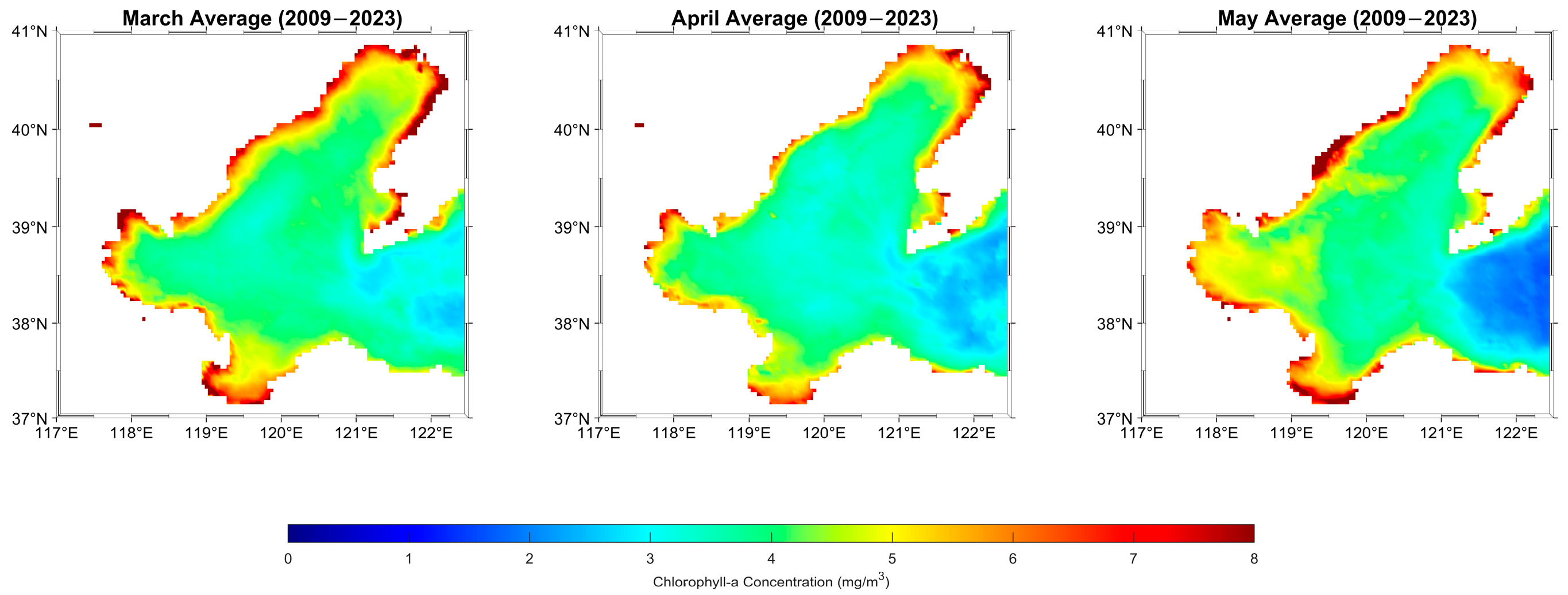
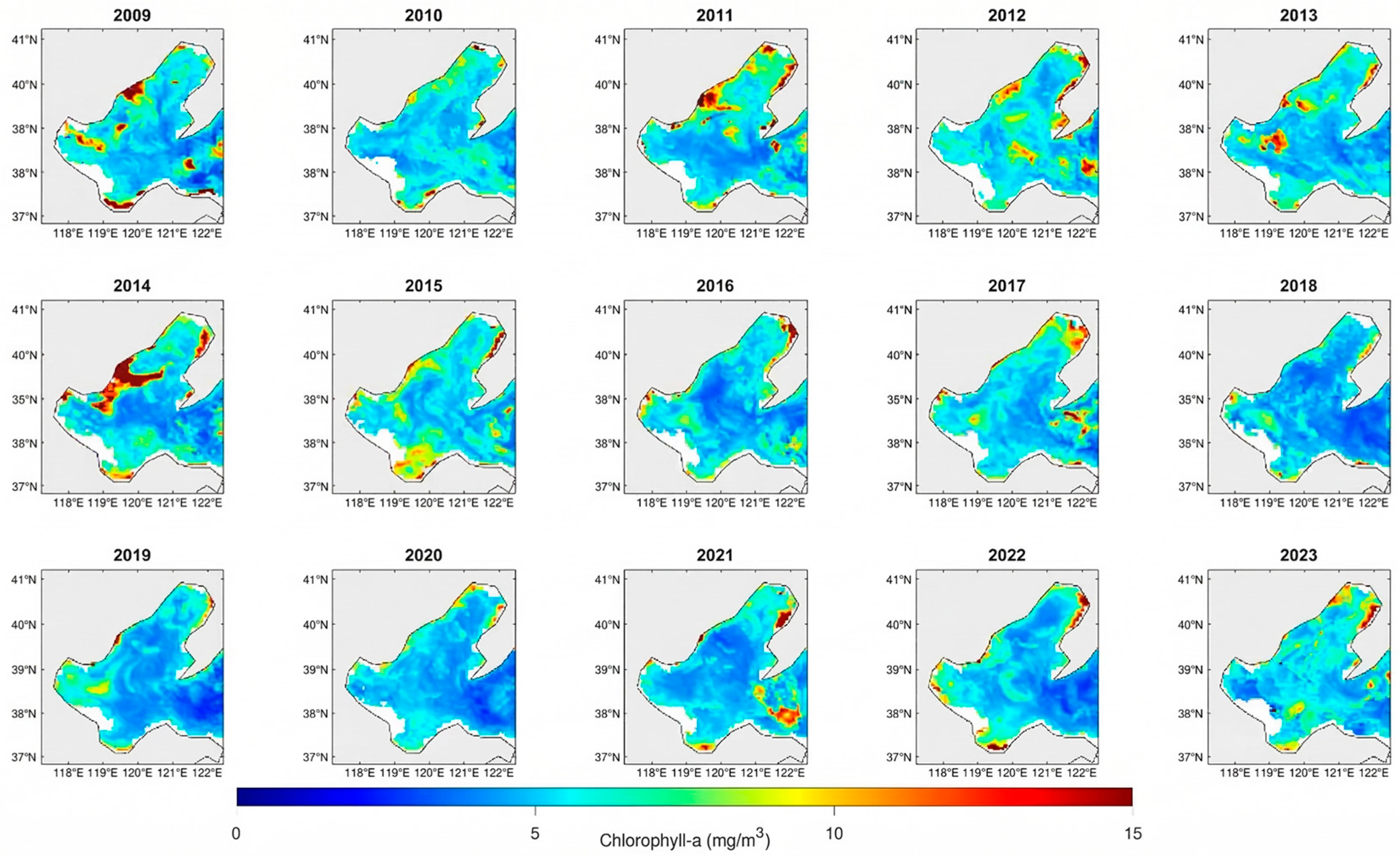
Chl-a concentration serves as a proxy for phytoplankton biomass and indicates the intensity of spring blooms. The multi-year average spring (March–May) Chl-a distribution in the BS from 2009 to 2023 (Figure 2) reveals a distinct spatial pattern characterized by high concentrations in nearshore waters and lower values in offshore regions. High-value zones were predominantly concentrated in the nearshore waters of LDB, Bohai Bay, and Laizhou Bay, where concentrations persistently exceeded 5 mg/m³. Given the exceptionally high background Chl-a average of the Bohai Sea (~4.5 mg/m³) [12]. The areas with Chl-a concentrations exceeding 5 mg/m³ effectively highlight severe, above-average phytoplankton hotspots driven by coastal eutrophication. We looked at the 15-year period of spring Chl-a peaks. Their spatial pattern (Figure 3) showed a clear nearshore distribution. The ice-covered regions of the LDB exhibit pronounced peaks. This shows high bloom intensity in these waters affected by ice. Direct satellite observations revealed highly localized high-concentration hotspots in specific years, such as along the Qinhuangdao coast in 2011 and 2014, and near the inner Bohai Bay in 2009, 2014, and 2022. These visual findings align with previous in situ observations [27,28]. Due to the resolution limits of the regional nutrient reanalysis data, direct quantification of these fine-scale chemical drivers is not feasible here. Instead, based on their spatial association with localized winter sea-ice presence, we hypothesize that these hotspots are fueled by localized nutrient enrichment from winter river discharge and coastal thawing. Together with increasing spring temperatures and light availability, this hypothesized nutrient pulse likely promotes the rapid phytoplankton growth observed in the satellite record.

3.1.2. Spatiotemporal Characteristics of Spring Bloom Peak Timing

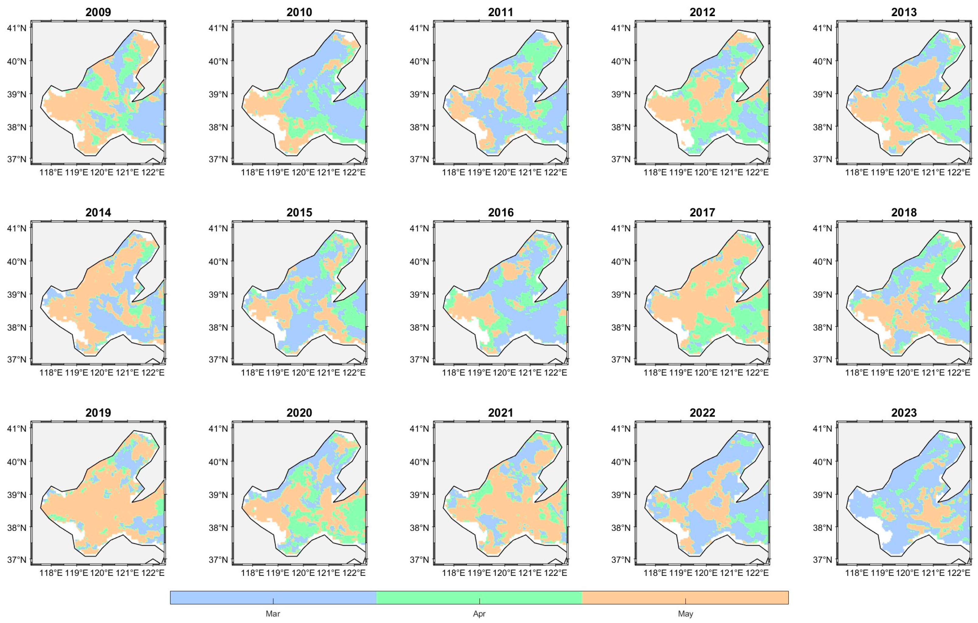
Figure 4 illustrates the spatial distribution of spring Chl-a peak timing (Bloom DOY) in the Bohai Sea in 2009–2023, highlighting the dominant timing of bloom occurrence and regional contrasts. To quantitatively illustrate these temporal patterns, the distributions of peak bloom timing for the primary subregions are summarized in

Table 1. Quantitative distribution of spring bloom peak timing (day of year) across major subregions (2009–2023).

Subregion	Median Peak DOY	Standard Deviation (Days)
Liaodong Bay	99	±8.5
Bohai Bay	125	±15.0
Laizhou Bay	104	±14.6

. Overall, pronounced temporal offsets in spring bloom peak timing were observed among different subregions. Blooms in the northern and central parts of LDB generally peaked earliest in March–April (median DOY of 99 ± 8.5 days), whereas those in Bohai Bay (median DOY of 125 ± 15.0 days) and Laizhou Bay (median DOY of 104 ± 14.6 days) predominantly reached their maxima in April–May. In some individual years (e.g., 2014, 2017, and 2019), relatively delayed bloom peaks, approaching May, occurred along the marginal areas of LDB. However, the Bloom DOY in the core region of LDB remained earlier than that in the southern bays. This spatiotemporal pattern reflects asynchronous seasonal evolution of sea-ice melt and upper-ocean temperature across the Bohai Sea. From a spatial gradient perspective, the spring bloom peak exhibits a clear north–south contrast, with earlier blooms in the northern regions and progressively later blooms toward the south. In addition, Bloom DOY generally occurs earlier in the outer parts of each bay (defined here as the deeper waters transitioning toward the Central Bohai Basin) than in their inner coastal regions (the shallow, tightly enclosed coastal margins).

3.2. Variability of Winter Sea Ice Across Different Temporal Scales

3.2.1. Interannual Variability

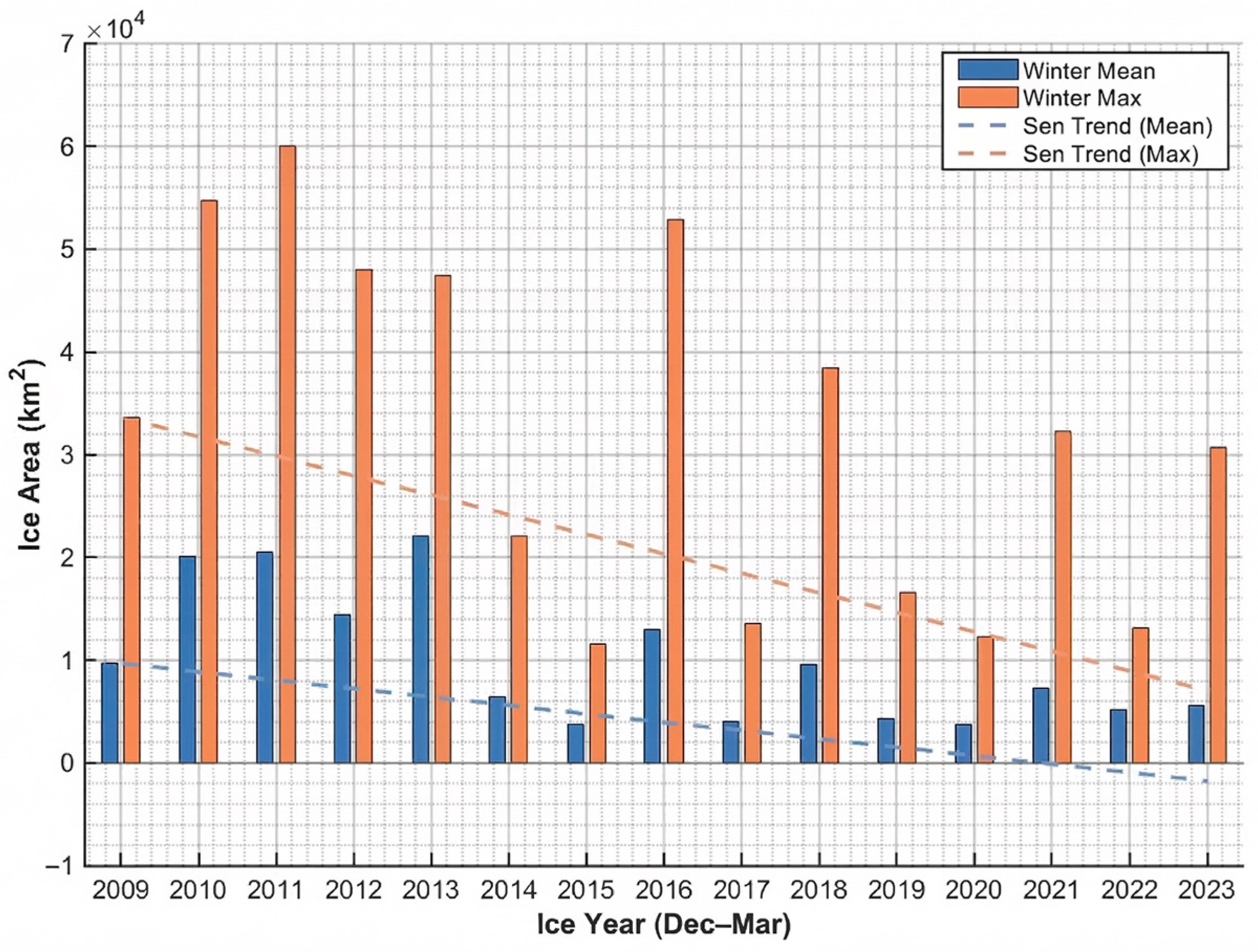
Based on the interannual variability of sea-ice area in the Bohai Sea in 2009–2023 (Figure 5), pronounced year-to-year fluctuations are evident, superimposed on a statistically significant long-term declining trend. The annual mean sea-ice area decreased at a rate of −816.99 km² yr⁻¹ (Sen’s slope; 95% CI: −1643.58 to −8.98 km² yr⁻¹; modified Mann–Kendall p = 0.0377). Similarly, the annual maximum sea-ice area declined at −1900.00 km² yr⁻¹ (95% CI: −4252.80 to −116.00 km² yr⁻¹; p = 0.0377), indicating a significant reduction in peak winter ice coverage over the study period.

Relatively extensive sea-ice conditions persisted in 2010–2013, with the annual maximum sea-ice area peaking at approximately 6.0 × 10⁴ km² in 2011. The second highest values occurred in 2010 and 2016. In contrast, 2015 and 2017 represent typical light-ice years, with annual maximum sea-ice areas of only about 1.1 × 10⁴ km² and 2.1 × 10⁴ km², respectively. Notably, the intervening year 2016 exhibited an anomalously high ice extent, with an annual maximum sea-ice area reaching 5.3 × 10⁴ km²—approximately five times that of 2015—and an annual mean sea-ice area increasing to 1.3 × 10⁴ km². Despite the pronounced ice conditions in 2016, the mean sea-ice extent remained lower than that in 2011, suggesting that the extreme ice coverage in 2016 was more likely driven by short-lived, high-intensity cold events rather than persistently low temperatures throughout the entire winter season.

3.2.2. Monthly Variability

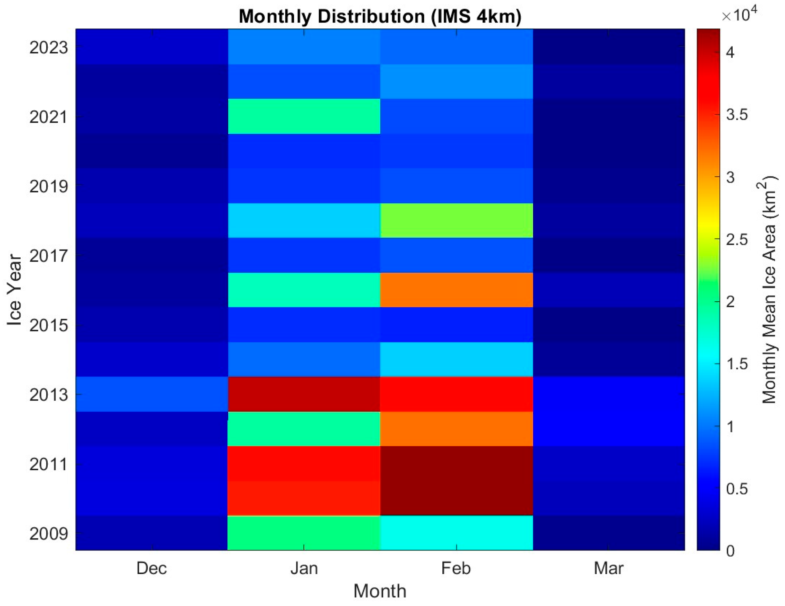
Sea ice in the Bohai Sea exhibits pronounced seasonal growth and decay (Figure 6), with the primary ice-covered period extending from December to the following March. The peak ice season typically occurs in January or February, when monthly mean sea-ice area reaches its highest values. During the peak seasons of 2010, 2011, and 2013, monthly sea-ice area exceeded 4.0 × 10⁴ km², followed by rapid melting in March. Figure 6 clearly illustrates distinct high-value bands in 2010–2013 and 2016, consistent with the interannual variability described above. This pattern of rapid formation, short-lived persistence, and abrupt melting indicates a pulsed, short-duration sea-ice regime. Such temporal concentration of meltwater release provides a physical basis for subsequent analyses of its transient impacts on spring physical–ecological conditions.

3.3. Spatiotemporal Relationships Between Sea Ice and Phytoplankton Blooms

Table 2. Spatially resolved Sen’s slope and Mann–Kendall significance between sea-ice parameters and spring bloom characteristics (2009–2023).

Subregion	Ice Variable	Bloom Variable	Sen’s Slope	p-Value	Samples (n)
Whole Bohai	Max Area	Peak DOY	0.00	1.00	15
Whole Bohai	Max Area	Peak Chl	0.00	0.50	15
Whole Bohai	Mean Area	Peak DOY	0.00	0.70	15
Whole Bohai	Mean Area	Peak Chl	0.00	0.50	15
Whole Bohai	Melt DOY	Peak DOY	0.68	0.58	14
Whole Bohai	Melt DOY	Peak Chl	−0.00	1.00	14
Liaodong Bay	Max Area	Peak DOY	−0.00	0.92	15
Liaodong Bay	Max Area	Peak Chl	−0.00	0.92	15
Liaodong Bay	Mean Area	Peak DOY	0.00	0.32	15
Liaodong Bay	Mean Area	Peak Chl	0.00	0.92	15
Liaodong Bay	Melt DOY	Peak DOY	2.67	0.03	15
Liaodong Bay	Melt DOY	Peak Chl	−0.03	0.88	15
Bohai Bay	Max Area	Peak DOY	0.00	0.65	7
Bohai Bay	Max Area	Peak Chl	−0.00	0.45	7
Bohai Bay	Mean Area	Peak DOY	0.00	0.65	7
Bohai Bay	Mean Area	Peak Chl	−0.00	0.45	7
Bohai Bay	Melt DOY	Peak DOY	0.45	0.71	7
Bohai Bay	Melt DOY	Peak Chl	−0.01	0.71	7
Laizhou Bay	Max Area	Peak DOY	0.00	1.00	4
Laizhou Bay	Max Area	Peak Chl	−0.00	1.00	4
Laizhou Bay	Mean Area	Peak DOY	0.02	1.00	4
Laizhou Bay	Mean Area	Peak Chl	−0.00	1.00	4
Laizhou Bay	Melt DOY	Peak DOY	−0.24	1.00	4
Laizhou Bay	Melt DOY	Peak Chl	−0.05	1.00	4

presents the results of the modified Mann–Kendall (M-K) analysis and Sen’s slope estimations for the relationships between sea-ice parameters and spring bloom metrics across different subregions of the Bohai Sea. To ensure statistical rigor and avoid artificial inflation of significance due to spatial autocorrelation, all analyses were conducted using regionally averaged annual time series.

At the scale of the entire Bohai Sea, no statistically significant monotonic relationships were detected between sea-ice area, melt timing, and bloom characteristics (p > 0.05), indicating a limited basin-wide statistical response of spring blooms to sea-ice variability. In contrast, Liaodong Bay (LDB) exhibited a significant positive relationship between sea-ice melt date and bloom peak timing (Sen’s slope = 2.67 days/day, p = 0.0275). This result suggests that a one-day delay in sea-ice retreat corresponds to an approximately 2.7-day delay in the bloom peak. This strong phenological control highlights the critical role of ice melt timing in this ice-dominated northern subregion. However, no significant relationships were found between sea-ice area and bloom metrics in LDB, suggesting that bloom phenology is more sensitive to the timing of ice melt than to the total ice extent.

In Bohai Bay and Laizhou Bay, no statistically significant relationships were detected. It should be noted that the effective sample sizes in these two subregions were considerably smaller (n = 7 and n = 4, respectively). This reduction is primarily due to the fact that during several winters in the 2009–2023 study period, IMS satellite observations recorded no detectable sea ice in these southern areas. The reduced sample size limits the statistical power of the analysis and partly explains the absence of significant associations in these regions.

Overall, the influence of sea ice on spring blooms exhibits pronounced regional heterogeneity. A statistically robust ice–phenology linkage was identified only in Liaodong Bay, reflecting a clear north–south contrast in ice-driven ecological responses.

3.4. GAMs Analysis of Dominant Drivers of Spring Phytoplankton Blooms

Based on the correlation analysis presented in the previous section, we found that in LDB, the sea-ice melt date was significantly positively correlated with bloom peak timing, whereas in Bohai Bay and Laizhou Bay, the limited winter sea-ice coverage resulted in no clear correlation between these variables. To further quantify the relative contributions of multiple environmental variables within a nonlinear predictive framework, Bohai Bay and Laizhou Bay were combined as the southern Bohai Sea for the subsequent GAM analysis.

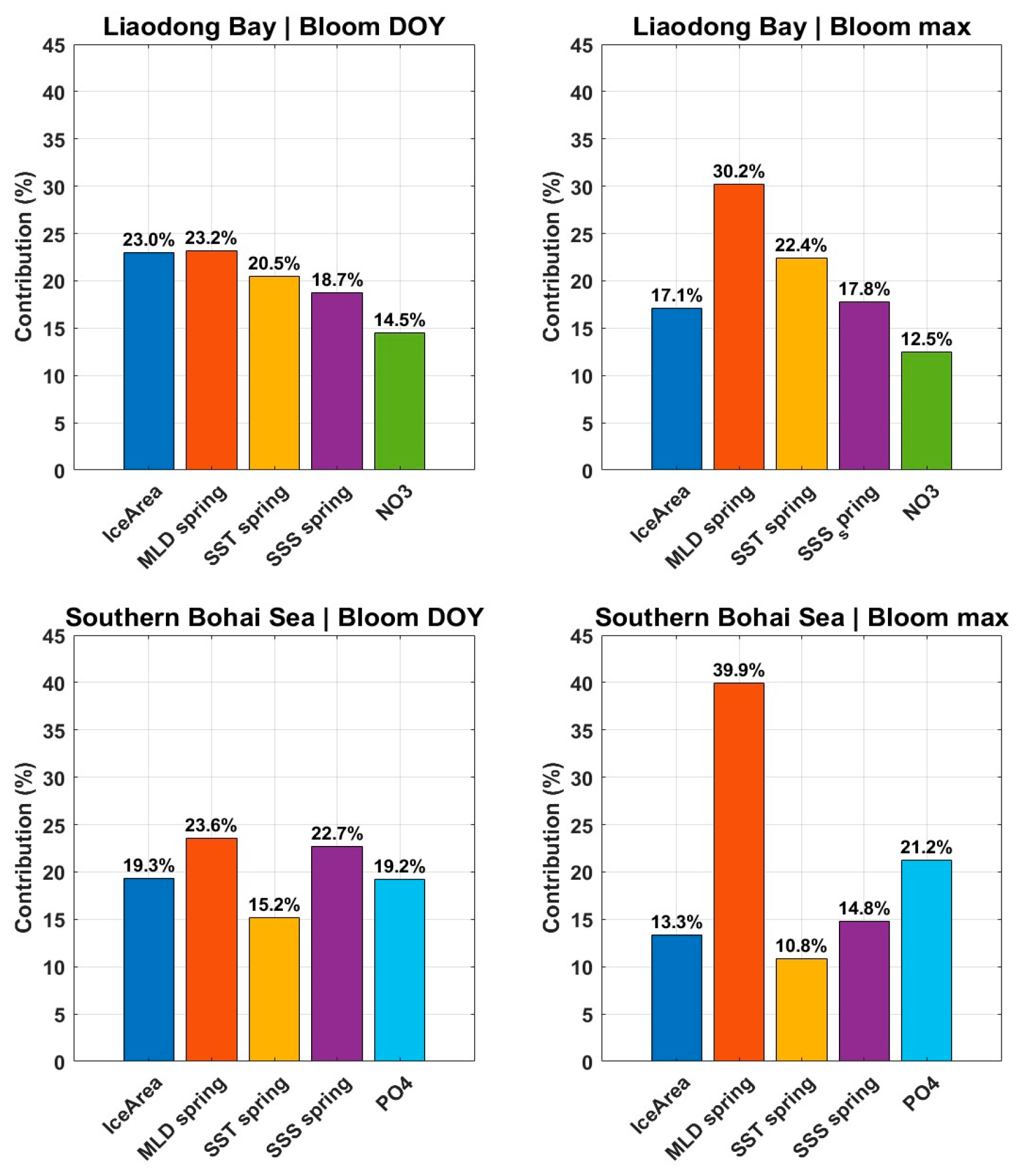
GAM results (Figure 7,

Table 3. Summary of generalized additive model (GAM) predictor selection (VIF), relative importance, and cross-validated model performance for spring bloom timing and intensity in Liaodong Bay and the southern Bohai Sea.

Region and Response Variable	Explanatory Variables	VIF	Relative Importance (%)	Model Performance (Cross-Validated)
Liaodong Bay
Bloom DOY	MLD spring	<5	23.20%	R2 = 0.32
	Ice area	<5	23.00%	RMSE = 15.63 days
	SST spring	<5	20.50%
	SSS spring	<5	18.70%
	NO3	<5	14.50%
Bloom max	MLD spring	<5	30.20%	R2 = 0.29
	SST spring	<5	22.40%	RMSE = 1.48 mg/m3
	SSS spring	<5	17.80%
	Ice area	<5	17.10%
	NO3	<5	12.50%
Southern Bohai Sea
Bloom DOY	MLD spring	<5	23.60%	R2 = 0.38
	SSS spring	<5	22.70%	RMSE = 22.25 days
	Ice area	<5	19.30%
	PO4	<5	19.20%
	SST spring	<5	15.20%
Bloom max	MLD spring	<5	39.90%	R2 = 0.41
	PO4	<5	21.20%	RMSE = 0.31 mg/m3
	SSS spring	<5	14.80%
	Ice area	<5	13.30%
	SST spring	<5	10.80%

) indicate pronounced spatial heterogeneity in the environmental factors associated with spring phytoplankton blooms in the BS. In Liaodong Bay, both bloom timing and bloom intensity exhibit stronger statistical associations with physical variables. For the bloom peak timing (Bloom DOY), spring mixed layer depth (23.2%) and sea-ice area (23.0%) show the highest relative predictive contributions, followed by spring sea surface temperature (20.5%), salinity (18.7%), and nitrate (14.5%). For bloom peak intensity (Bloom max), mixed layer depth again shows the largest relative importance (30.2%), with SST (22.4%), salinity (17.8%), sea-ice area (17.1%), and nitrate (12.5%) contributing to varying degrees. The cross-validated model performance indicates moderate predictive skill (R² = 0.32, RMSE = 15.63 days for Bloom DOY; R² = 0.29, RMSE = 1.48 mg/m³ for Bloom max). These results suggest that variability in upper-ocean physical structure is statistically closely associated with interannual bloom dynamics in LDB.

In the southern Bohai Sea, the distribution of predictor importance appears more balanced, implying the joint influence of physical and biogeochemical factors. For bloom peak timing, mixed layer depth (23.6%) and salinity (22.7%) exhibit comparable contributions, followed by sea-ice area (19.3%), phosphate (19.2%), and SST (15.2%). For bloom intensity, mixed layer depth shows the strongest predictive contribution (39.9%), while phosphate (21.2%), salinity (14.8%), sea-ice area (13.3%), and SST (10.8%) contribute to a lesser extent. The predictive performance is relatively higher than in LDB (R² = 0.38, RMSE = 22.25 days for Bloom DOY; R² = 0.41, RMSE = 0.31 mg/m³ for Bloom max). These statistical results indicate a likely influence of Yellow River discharge in the southern region. Multiple mechanisms, including riverine input, stratification, and nutrient availability, appear to jointly influence bloom dynamics.

These statistical results indicate a likely influence of Yellow River discharge in the southern region. Multiple mechanisms, including riverine input, stratification, and nutrient availability, appear to jointly influence bloom dynamics.

3.5. Dominant Drivers of Spring Stratification in Liaodong Bay

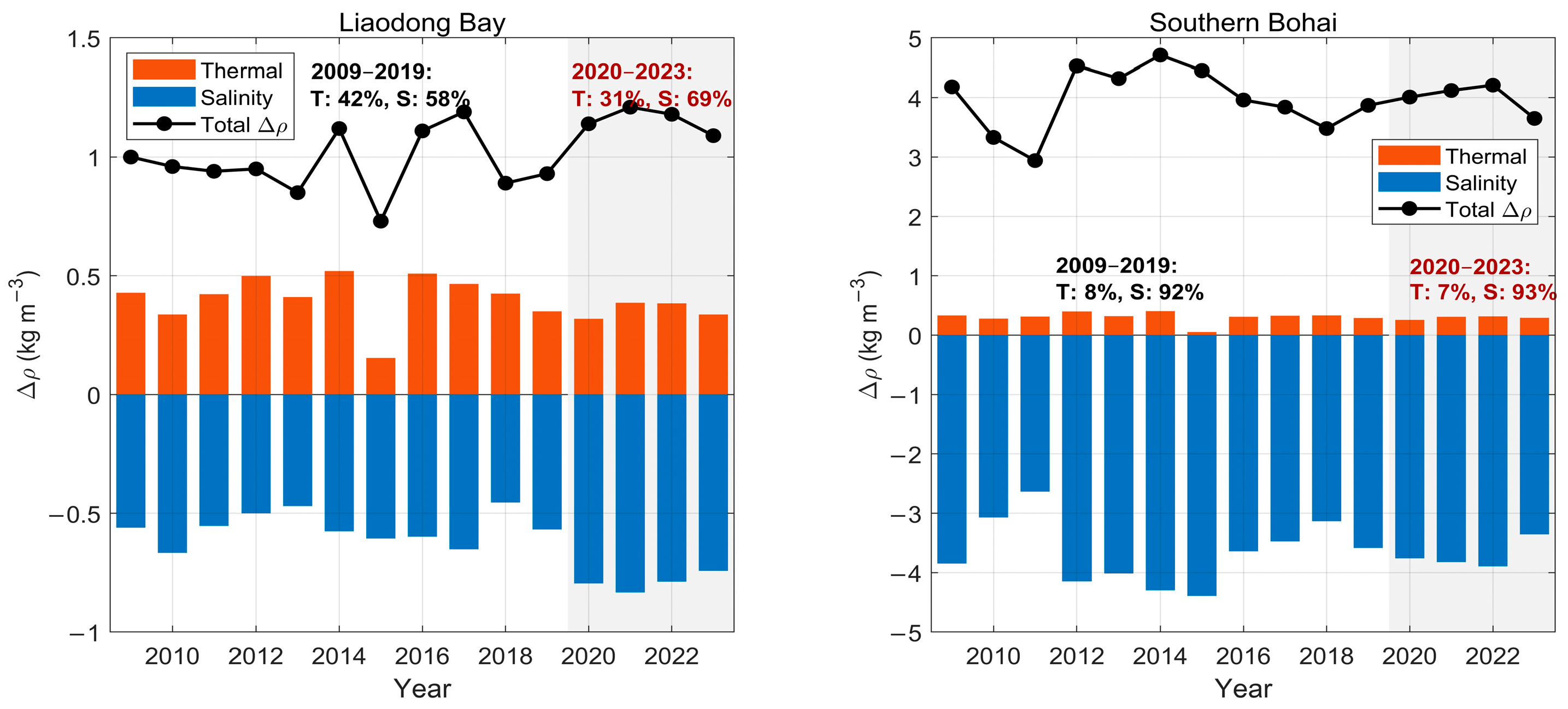
Previous GAM results indicated that spring phytoplankton blooms in LDB are strongly regulated by sea-ice extent and mixed layer depth. To further elucidate the physical mechanisms through which sea ice influences mixed layer depth, we analyzed temperature and salinity data from surface and bottom layers during spring (March–May) in 2009–2023. Density difference (Δρ) was calculated as an indicator of stratification intensity, and a linear decomposition into thermal and salinity contributions was performed (Figure 8,

Table 4. Statistical parameters of the linear decomposition of water stratification and the relative contributions of thermal and salinity effects in Liaodong Bay and Southern Bohai during spring (2009–2023).

Region	A Thermal	B Salinity	R2	Thermal Contribution	Salinity Contribution
Liaodong Bay	0.12	0.75	0.95	0.39	0.61
Southern Bohai	0.12	0.79	0.99	0.08	0.92

) to quantify the relative roles of different factors in controlling water column stability. This decomposition approach has been widely used in studies of mixed layer structure and water-column stratification [26,29,30].

The decomposition results indicate a salinity-dominated stratification pattern in the southern Bohai Sea. Given the hydrographic setting of this region, such stratification is likely influenced by freshwater inputs from the Yellow River. Although river discharge time series were not explicitly analyzed in the present study, this interpretation is consistent with recent numerical modeling studies. For example, Ju demonstrated that Yellow River runoff plays a dominant role in regulating the salinity distribution and the spatial extent of low-salinity zones in Laizhou Bay, thereby modulating upper-ocean density structure [31]. Salinity contributes about 92.4% on average to the total density difference (R² > 0.9), indicating a typical salinity-controlled stratification, which is consistent with previous studies [32]. The LDB shows a different situation. It is deeper, experiences stronger tidal mixing, and is covered by extensive sea ice in winter, resulting in a more complex stratification regime. Both thermal and dynamic factors play roles in controlling stratification. Our analysis further shows that, in Liaodong Bay, salinity still dominates, contributing about 60.7% on average to stratification. Our analysis shows details for Liaodong Bay. Salinity contributes about 60.7% on average to stratification. Temperature contributes about 39.3% to stratification. This differentiation mainly shows the modulation of freshwater pathways. Yellow River discharge and wind stress do this modulation [33]. There are also inherent differences among the bays. They are in a geographic–dynamic setting and energy balance [34].

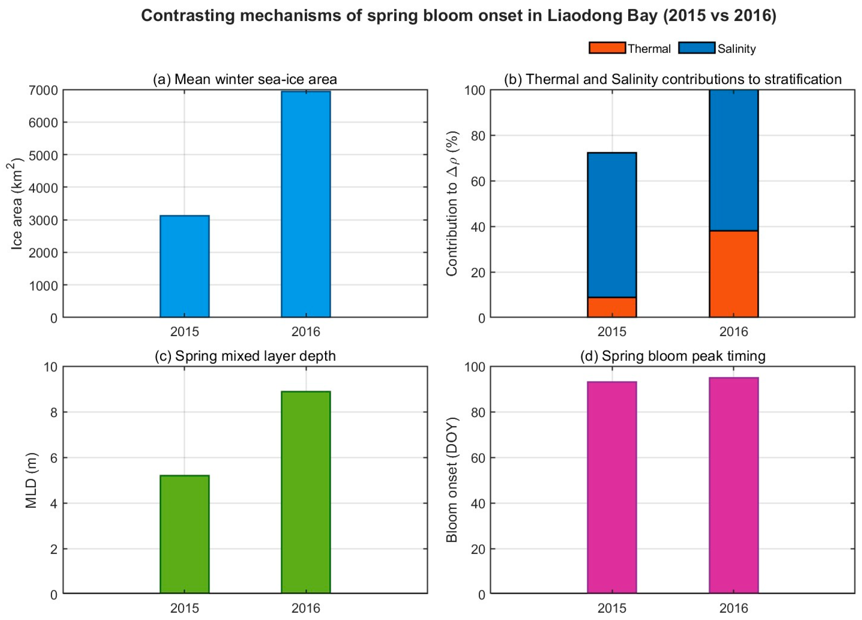
At the interannual scale, Δρ in both regions decreased markedly in spring 2015, with a minimal contribution from temperature, yet the bloom peak timing in Liaodong Bay (LDB) occurred approximately 27 days earlier in 2015 (DOY 93.01 ± 27.43) compared to 2014 (DOY 119.62 ± 33.14). This significant advancement is consistent with the transition to an exceptionally shallow mixed layer (5.21 m) observed in 2015, which satisfied Sverdrup’s critical depth criterion and triggered an earlier bloom outbreak despite the weak thermal stratification. Further analysis of LDB indicates a shift in stratification mechanisms around 2020. In 2009–2019, the relative contributions of temperature and salinity were approximately 42% and 58%, respectively; since 2020, salinity has increased to ~69%, while temperature contribution declined to ~31% (Figure 8). This shift likely reflects recent changes in freshwater fluxes in the Bohai Sea, such as enhanced precipitation and increased river discharge, which have altered the salinity structure [35]. The transition from joint thermal–salinity control to predominantly salinity-driven stratification suggests that the physical environment in LDB is evolving toward a more stable, strongly stratified state, a pattern similarly observed in other semi-enclosed seas strongly influenced by terrestrial freshwater inputs [31].

4. Discussion

4.1. Winter Sea-Ice Effects on Spring Phytoplankton Blooms

Comprehensive correlation analysis, GAM modeling, and density decomposition collectively indicate significant spatial heterogeneity in the drivers of spring phytoplankton blooms in the Bohai Sea. LDB exhibits a typical physically dominated regime, whereas the southern Bohai Sea is regulated by a combination of physical and biogeochemical factors.

In Liaodong Bay, winter sea-ice melt is the key physical factor controlling bloom peak timing. GAM results explicitly show that sea-ice extent and mixed layer depth (MLD) jointly regulate both bloom peak timing and peak intensity. Specifically, for bloom peak timing, their combined contribution reaches 46.2% (Ice Area: 23.0%, MLD: 23.2%). Similarly, for bloom peak intensity, their combined contribution accounts for 47.3% (Ice Area: 17.1%, MLD: 30.2%). Meltwater from sea-ice decay is crucial for establishing strong stratification, which lowers surface salinity and maintains a shallow mixed layer, promoting phytoplankton accumulation in the well-illuminated surface layer [36]. This stable stratification significantly shoals the MLD. Although photosynthetically active radiation (PAR) and euphotic depth were not directly measured in the present study, the physical compression of the mixed layer likely increases light availability for phytoplankton trapped in the surface layer. This inferred pathway is robustly supported by recent literature on ice-edge blooms [37], which demonstrates that meltwater-induced stratification fundamentally creates favorable light conditions, leading to earlier and more intense blooms. Therefore, our findings remain highly consistent with Sverdrup’s critical depth theory: strong salinity stratification suppresses vertical turbulent mixing, which is hypothesized to confine the MLD within the euphotic zone and relieve light limitation.

To further highlight the influence of contrasting ice conditions, we compared two consecutive years within the Liaodong Bay (LDB) spatial domain (Figure 9): 2016 (a heavy ice year) and 2015 (a light ice year). This comparison confirms the nonlinear characteristics of the bloom response. In 2016, extensive ice melt formed a strong salinity stratification, providing an efficient physical pathway for MLD shoaling. Conversely, 2015 exhibited no obvious meltwater layer. However, based on the CMEMS reanalysis data, the spring (March–May) atmospheric and hydrographic conditions spatially averaged across the LDB were anomalously cold. The mean spring temperature in 2015 was 3.19 ± 0.65 °C (compared to 8.42 ± 0.74 °C in 2016). This cold anomaly reduced wind-driven mixing and maintained an extremely shallow regional MLD of 5.21 ± 10.77 m. The large spatial standard deviation of MLD reflects the steep hydrodynamic gradient from the shallow inner bay to the deeper central basin. Nevertheless, this predominantly shallow MLD robustly satisfied the Sverdrup criterion, initiating an early bloom despite the weak thermal stratification. Ultimately, the timing of the bloom peak depends critically on MLD shoaling; while sea-ice melt is the primary driver, anomalously cold conditions can occasionally provide a secondary physical pathway to achieve this stable state.

4.2. Spatial Heterogeneity of Bloom Drivers in the Southern Bohai Sea

The southern Bohai Sea exhibits a fundamentally different regime. Unlike the extensive coverage in LDB, winter sea ice in the southern bays is intermittent and geographically restricted (e.g., completely absent in several years during the 2009–2023 period). Consequently, this localized meltwater input is spatially and temporally insufficient to generate a basin-wide, stable halocline. The overarching stratification in the south is instead dominated by massive freshwater discharge from the Yellow River. However, this does not imply that sea ice is ecologically irrelevant in the south. In fact, our updated GAM results highlight that the sea-ice area still maintains a notable contribution to bloom peak timing (19.3%) and intensity (13.3%). This suggests that in the specific cold years and coastal margins where ice does form, localized meltwater release still actively modulates bloom dynamics. Overall, bloom variability in the southern Bohai Sea is co-regulated by a complex combination of physical mixing, intermittent sea-ice effects, and riverine nutrient input (with PO4 showing a strong 21.2% relative contribution to bloom intensity).

It should be noted, however, that the apparent nutrient-driven regime in the southern Bohai Sea remains subject to data limitations. The CMEMS reanalysis data employed here, though useful for regional trends, have not been extensively validated in situ for this eutrophic coastal zone. Because global models often struggle to resolve the episodic, high-concentration nutrient inputs from the Yellow River, our GAM results regarding nutrient control should be considered preliminary. While they indicate a shift toward biogeochemical regulation in the south, high-resolution field observations are ultimately required to corroborate these localized processes.

4.3. Limitations and Perspectives

Additionally, it is important to acknowledge the limitations regarding the methodology used to define spring blooms in this study. By defining bloom intensity as the maximum Chl-a concentration, this approach intrinsically simplifies the complex temporal dynamics of phytoplankton phenology. While robust against the severe early-spring optical noise typical in this region, it overlooks bloom duration, shifts in the seasonal baseline, and the potential occurrence of multiple secondary blooms. Future studies incorporating high-frequency geostationary satellite data are recommended to capture the full phenological life cycle.

In conclusion, while the melt–stratification–bloom mechanism is established in polar oceans, our study reveals distinct new characteristics for the mid-latitude Bohai Sea:

(1)

Unlike polar regions where severe under-ice light limitation dictates that blooms only occur post-retreat, the adequate background radiation in the mid-latitude Liaodong Bay means that light only becomes sufficient when the MLD is physically compressed into the euphotic zone by meltwater.

(2)

We quantitatively demonstrated that spring stratification in the ice-covered Liaodong Bay is predominantly salinity-driven rather than thermally driven. This completely updates the conventional assumption that mid-latitude spring stratification relies primarily on surface warming.

(3)

Our GAM analysis highlights a stark spatial heterogeneity unique to this marginal sea. While the southern Bohai Sea is largely nutrient-controlled (with nitrate playing a major role), the ice-covered Liaodong Bay is overwhelmingly physically controlled. Specifically, MLD acts as the direct physical driver governing light availability, while sea-ice melt serves as the essential forcing mechanism that compresses the MLD into the euphotic zone. This demonstrates that sea ice acts as a localized, dominant physical switch in an otherwise nutrient-complex coastal system.

In summary, this complete melting–freshening–stratification–light coupling chain explicitly defines the ‘new physical perspective’ highlighted in this study. Our quantitative density decomposition firmly establishes that the physical foundation of the Liaodong Bay spring bloom is a salinity-dominated dynamic process, rather than the thermally-driven warming typical of other mid-latitude marginal seas. Furthermore, distinct from polar mechanisms where ice melt primarily serves to relieve light attenuation, the critical ecological role of sea-ice in this mid-latitude bay is providing a rapid freshwater flux that suppresses turbulent mixing and compresses the MLD. This distinct physically-driven regime enriches our understanding of how mid-latitude sea-ice ecosystems uniquely respond to seasonal and interannual climatic variations.

5. Conclusions

This study uses data from 2009 to 2023. It explains spring phytoplankton blooms’ spatiotemporal differences in the BS. It also provides statistical evidence consistent with the physical–biological coupling mechanisms driven by sea-ice melting. The main conclusions are as follows:

(1)

Winter sea-ice area in the Bohai Sea exhibits a significant long-term declining trend superimposed with substantial interannual variability. The ecological influence of sea ice displays pronounced regional heterogeneity. In Liaodong Bay (LDB), sea-ice melt timing is significantly and positively associated with peak bloom timing (Sen’s slope = 2.67 days/day). The southern Bohai Sea exhibits a relatively stronger statistical association with nutrient variability, although this inference is subject to uncertainties inherent in global reanalysis data in nearshore environments.

(2)

GAM results give clear information. Blooms in the LDB are predominantly associated with physical processes. The bloom peak timing is most strongly associated with MLD and sea-ice area, with relative contributions of 23.2% and 23.0%, respectively. Bloom peak intensity is predominantly explained by MLD, contributing 30.2%. The southern BS exhibits a different pattern, where blooms show a stronger dependence on nutrient conditions.

(3)

LDB has a clear coupling chain: melting–freshening–stratification–light. Sea-ice meltwater lowers surface salinity and creates a strong halocline, which suppresses vertical mixing and keeps MLD within the euphotic zone. This process eases light limitation. It also starts bloom outbreaks. Salinity contributes about 60% to the density difference. Although initial water temperatures during the melting phase are low, this highly stable structure allows the surface to warm quickly, ensuring blooms effectively develop and persist.

References

1. Shi, J.; Liu, Y.; Mao, X.; Guo, X.; Wei, H.; Gao, H. Interannual Variation of Spring Phytoplankton Bloom and Response to Turbulent Energy Generated by Atmospheric Forcing in the Central Southern Yellow Sea of China: Satellite Observations and Numerical Model Study. Cont. Shelf Res. 2017, 143, 257–270. [Google Scholar] [CrossRef] [Scilit]
2. Townsend, D.W.; Keller, M.D.; Sieracki, M.E.; Ackleson, S.G. Spring Phytoplankton Blooms in the Absence of Vertical Water Column Stratification. Nature 1992, 360, 59–62. [Google Scholar] [CrossRef] [Scilit]
3. Chiswell, S.M.; Calil, P.H.R.; Boyd, P.W. Spring Blooms and Annual Cycles of Phytoplankton: A Unified Perspective. J. Plankton Res. 2015, 37, 500–508. [Google Scholar] [CrossRef] [Scilit]
4. Chen, Y.; Wang, L.; Liu, Z.; Su, D.; Wang, Y.; Qi, Y. Biodiversity and Interannual Variation of Harmful Algal Bloom Species in the Coastal Sea of Qinhuangdao, China. Life 2023, 13, 192. [Google Scholar] [CrossRef] [Scilit]
5. Li, X.-Y.; Yu, R.-C.; Richardson, A.J.; Sun, C.; Eriksen, R.; Kong, F.-Z.; Zhou, Z.-X.; Geng, H.-X.; Zhang, Q.-C.; Zhou, M.-J. Marked Shifts of Harmful Algal Blooms in the Bohai Sea Linked with Combined Impacts of Environmental Changes. Harmful Algae 2023, 121, 102370. [Google Scholar] [CrossRef] [Scilit]
6. Wei, Y.; Cui, H.; Hu, Q.; Bai, Y.; Qu, K.; Sun, J.; Cui, Z. Eutrophication Status Assessment in the Laizhou Bay, Bohai Sea: Further Evidence for the Ecosystem Degradation. Mar. Pollut. Bull. 2022, 181, 113867. [Google Scholar] [CrossRef] [Scilit]
7. Liu, S.; Li, G.; Liu, S.; Zhang, L.; Li, M.; Feng, Q.; Xing, L.; Yu, D.; Pan, Y. Impacts of Sea Ice on Suspended Sediment Transport during Heavy Ice Years in the Bohai Sea. Front. Mar. Sci. 2024, 11, 1411770. [Google Scholar] [CrossRef] [Scilit]
8. Wang, A.; Tang, M.; Zhao, Q.; Liu, Y.; Li, B.; Shi, Y.; Sui, J. Analysis of Sea Ice Parameters for the Design of an Offshore Wind Farm in the Bohai Sea. Ocean Eng. 2021, 239, 109902. [Google Scholar] [CrossRef] [Scilit]
9. Liu, C.; Gu, W.; Chao, J.; Li, L.; Yuan, S.; Xu, Y. Spatio-Temporal Characteristics of the Sea-Ice Volume of the Bohai Sea, China, in Winter 2009/10. Ann. Glaciol. 2013, 54, 97–104. [Google Scholar] [CrossRef] [Scilit]
10. Zhang, H.; Qiu, Z.; Sun, D.; Wang, S.; He, Y. Seasonal and Interannual Variability of Satellite-Derived Chlorophyll-a (2000–2012) in the Bohai Sea, China. Remote Sens. 2017, 9, 582. [Google Scholar] [CrossRef] [Scilit]
11. Du, Y.; Zhang, X.; Ma, S.; Yao, N. Chlorophyll-a Concentration Variations in Bohai Sea: Impacts of Environmental Complexity and Human Activities Based on Remote Sensing Technologies. Big Data Res. 2024, 36, 100440. [Google Scholar] [CrossRef] [Scilit]
12. Zhang, K.; Zhao, X.; Xue, J.; Mo, D.; Zhang, D.; Xiao, Z.; Yang, W.; Wu, Y.; Chen, Y. The Temporal and Spatial Variation of Chlorophyll a Concentration in the China Seas and Its Impact on Marine Fisheries. Front. Mar. Sci. 2023, 10, 1212992. [Google Scholar] [CrossRef] [Scilit]
13. Ardyna, M.; Mundy, C.J.; Mayot, N.; Matthes, L.C.; Oziel, L.; Horvat, C.; Leu, E.; Assmy, P.; Hill, V.; Matrai, P.A.; et al. Under-Ice Phytoplankton Blooms: Shedding Light on the “Invisible” Part of Arctic Primary Production. Front. Mar. Sci. 2020, 7, 608032. [Google Scholar] [CrossRef] [Scilit]
14. Hill, V.J.; Light, B.; Steele, M.; Zimmerman, R.C. Light Availability and Phytoplankton Growth Beneath Arctic Sea Ice: Integrating Observations and Modeling. J. Geophys. Res. Ocean. 2018, 123, 3651–3667. [Google Scholar] [CrossRef] [Scilit]
15. Sverdrup, H.U. On Conditions for the Vernal Blooming of Phytoplankton. J. Cons. Int. Explor. Mer. 1953, 18, 287–295. [Google Scholar] [CrossRef] [Scilit]
16. Douglas, C.C.; Briggs, N.; Brown, P.; MacGilchrist, G.; Naveira Garabato, A. Exploring the Relationship between Sea Ice and Phytoplankton Growth in the Weddell Gyre Using Satellite and Argo Float Data. Ocean Sci. 2024, 20, 475–497. [Google Scholar] [CrossRef] [Scilit]
17. Castagno, A.P.; Wagner, T.J.W.; Cape, M.R.; Lester, C.W.; Bailey, E.; Alves-de-Souza, C.; York, R.A.; Fleming, A.H. Increased Sea Ice Melt as a Driver of Enhanced Arctic Phytoplankton Blooming. Glob. Change Biol. 2023, 29, 5087–5098. [Google Scholar] [CrossRef] [Scilit]
18. Oldenburg, E.; Popa, O.; Wietz, M.; von Appen, W.-J.; Torres-Valdes, S.; Bienhold, C.; Ebenhöh, O.; Metfies, K. Sea-Ice Melt Determines Seasonal Phytoplankton Dynamics and Delimits the Habitat of Temperate Atlantic Taxa as the Arctic Ocean Atlantifies. ISME Commun. 2024, 4, ycae027. [Google Scholar] [CrossRef] [Scilit]
19. Chen, C.-T.A. Chemical and Physical Fronts in the Bohai, Yellow and East China Seas. J. Mar. Syst. 2009, 78, 394–410. [Google Scholar] [CrossRef] [Scilit]
20. Zhai, W.; Zhao, H.; Su, J.; Liu, P.; Li, Y.; Zheng, N. Emergence of Summertime Hypoxia and Concurrent Carbonate Mineral Suppression in the Central Bohai Sea, China. J. Geophys. Res. Biogeosciences 2019, 124, 2768–2785. [Google Scholar] [CrossRef] [Scilit]
21. Park, K.-A.; Kang, C.-K.; Kim, K.-R.; Park, J.-E. Role of Sea Ice on Satellite-Observed Chlorophyll-a Concentration Variations during Spring Bloom in the East/Japan Sea. Deep. Sea Res. Part I Oceanogr. Res. Pap. 2014, 83, 34–44. [Google Scholar] [CrossRef] [Scilit]
22. Nicholson, S.-A.; Ryan-Keogh, T.J.; Thomalla, S.J.; Chang, N.; Smith, M.E. Satellite-Derived Global-Ocean Phytoplankton Phenology Indices. Earth Syst. Sci. Data 2025, 17, 1959–1975. [Google Scholar] [CrossRef] [Scilit]
23. Blondeau-Patissier, D.; Gower, J.F.R.; Dekker, A.G.; Phinn, S.R.; Brando, V.E. A Review of Ocean Color Remote Sensing Methods and Statistical Techniques for the Detection, Mapping and Analysis of Phytoplankton Blooms in Coastal and Open Oceans. Prog. Oceanogr. 2014, 123, 123–144. [Google Scholar] [CrossRef] [Scilit]
24. Zhou, B.; Shi, K.; Wang, W.; Zhang, D.; Qin, B.-Q.; Zhang, Y.; Dong, B.; Shang, M.S. Phytoplankton Succession Phenology Trends in the Backwaters of the Three Gorges Reservoir in China and Their Drivers: Results from Satellite Observations. Ecol. Indic. 2022, 143, 109435. [Google Scholar] [CrossRef] [Scilit]
25. Brown, L.C.; Howell, S.E.L.; Mortin, J.; Derksen, C. Evaluation of the Interactive Multisensor Snow and Ice Mapping System (IMS) for Monitoring Sea Ice Phenology. Remote Sens. Environ. 2014, 147, 65–78. [Google Scholar] [CrossRef] [Scilit]
26. de Boyer Montégut, C.; Madec, G.; Fischer, A.S.; Lazar, A.; Iudicone, D. Mixed Layer Depth over the Global Ocean: An Examination of Profile Data and a Profile-Based Climatology. J. Geophys. Res. Oceans 2004, 109, C12003. [Google Scholar] [CrossRef] [Scilit]
27. Yao, P.; Lei, L.; Zhao, B.; Wang, J.; Chen, L. Spatial-Temporal Variation of Aureococcus anophagefferens Blooms in Relation to Environmental Factors in the Coastal Waters of Qinhuangdao, China. Harmful Algae 2019, 86, 106–118. [Google Scholar] [CrossRef] [Scilit] [PubMed]
28. Kong, F.; Yu, R.; Zhang, Q.; Yan, T.; Zhou, M. Pigment Characterization for the 2011 Bloom in Qinhuangdao Implicated “Brown Tide” Events in China. Chin. J. Oceanol. Limnol. 2012, 30, 361–370. [Google Scholar] [CrossRef] [Scilit]
29. Yu, L.; Weller, R.A. Objectively Analyzed Air–Sea Heat Fluxes for the Global Ice-Free Oceans (1981–2005). Bull. Am. Meteorol. Soc. 2007, 88, 527–540. [Google Scholar] [CrossRef] [Scilit]
30. Kara, A.B.; Rochford, P.A.; Hurlburt, H.E. Efficient and Accurate Bulk Parameterizations of Air–Sea Fluxes for Use in General Circulation Models. J. Atmos. Ocean. Technol. 2000, 17, 1421–1438. [Google Scholar] [CrossRef] [Scilit]
31. Ju, K.; Xiong, L.; Liu, T.; Li, Z.; Zhang, M. Numerical Analysis of the Influence of Runoff Input on Salinity Distribution and Its Mechanisms in Laizhou Bay. J. Mar. Sci. Eng. 2024, 12, 1858. [Google Scholar] [CrossRef] [Scilit]
32. Bian, C.; Jiang, W.; Pohlmann, T.; Sündermann, J. Hydrography-Physical Description of the Bohai Sea. J. Coast. Res. 2016, 74, 1–12. [Google Scholar] [CrossRef] [Scilit]
33. Wang, Q.; Guo, X.; Takeoka, H. Seasonal Variations of the Yellow River Plume in the Bohai Sea: A Model Study. J. Geophys. Res. Oceans 2008, 113, C12003. [Google Scholar] [CrossRef] [Scilit]
34. Simpson, J.H.; Hunter, J.R. Fronts in the Irish Sea. Nature 1974, 250, 404–406. [Google Scholar] [CrossRef] [Scilit]
35. Ji, F.; Xiong, X.; Yang, J.; Liu, Y.; Han, L.; Dong, M.; Xu, S. Local Freshwater Fluxes Determine Salinity Variations of the Bohai Sea: Based on 60 Years of Observations. Reg. Stud. Mar. Sci. 2024, 80, 103899. [Google Scholar] [CrossRef] [Scilit]
36. von Appen, W.-J.; Waite, A.M.; Bergmann, M.; Bienhold, C.; Boebel, O.; Bracher, A.; Cisewski, B.; Hagemann, J.; Hoppema, M.; Iversen, M.H.; et al. Sea-Ice Derived Meltwater Stratification Slows the Biological Carbon Pump: Results from Continuous Observations. Nat. Commun. 2021, 12, 7309. [Google Scholar] [CrossRef] [Scilit]
37. Lester, C.W.; Wagner, T.J.W.; McNamara, D.E.; Cape, M.R. The Influence of Meltwater on Phytoplankton Blooms Near the Sea-Ice Edge. Geophys. Res. Lett. 2021, 48, e2020GL091758. [Google Scholar] [CrossRef] [Scilit]
Figure 1. Map of the study area in the Bohai Sea, showing the major subregions including Liaodong Bay, Bohai Bay, Laizhou Bay, and the Bohai Strait.
Jmse 14 00540 g001
Figure 2. Fifteen-year mean spatial distribution of spring chlorophyll-a (Chl-a) concentration in the Bohai Sea (2009–2023).
Jmse 14 00540 g002
Figure 3. Interannual spatial distribution of spring maximum chlorophyll-a (Chl-a) concentration in the Bohai Sea from 2009 to 2023.
Jmse 14 00540 g003
Figure 4. Spatial distribution of the timing (phenology) of the spring chlorophyll-a (Chl-a) peak in the Bohai Sea from 2009 to 2023.
Jmse 14 00540 g004
Figure 5. Interannual variations of maximum and mean winter sea-ice extent in the Bohai Sea in 2009–2023.
Jmse 14 00540 g005
Figure 6. Heatmap of monthly mean sea-ice area (km2) in Bohai Sea.
Jmse 14 00540 g006
Figure 7. Relative contributions of spring environmental factors to bloom peak timing (Bloom DOY) and magnitude (Bloom max) in Liaodong Bay and the southern Bohai Sea, based on generalized additive models (GAMs).
Jmse 14 00540 g007
Figure 8. Interannual variations in surface-bottom density difference (Δρ) and the decomposition of thermal and salinity contributions in Liaodong Bay (left) and Southern Bohai (right) during spring from 2009 to 2023. The gray shaded area and red font color highlight the 2020–2023 period, indicating a recent shift towards predominantly salinity-driven stratification.
Jmse 14 00540 g008
Figure 9. Comparison of the physical–biological coupling mechanisms between a heavy ice year (2016) and a light ice year (2015) in Liaodong Bay: (a) Mean winter sea-ice area; (b) Relative contributions of thermal and salinity effects to spring water-column stratification (Δρ); (c) Spring mixed layer depth (MLD); and (d) Spring bloom peak timing (Bloom DOY).
Jmse 14 00540 g009