Reinforcement Learning-Based Sliding Mode Control of Underwater Vehicles with Bow Rudders and X-Stern Rudders

Abstract

This paper addresses the motion control for an x-rudder underwater vehicle, which features a bow rudder and four independent x-shaped stern rudders. To achieve coordinated operation of bow and stern rudders of the x-rudder underwater vehicle, the motion controller is divided into two parts: dynamic controller and control distributor. A model-free sliding mode parameter optimization control algorithm for underwater vehicles based on reinforcement learning (RL) is proposed. The proposed algorithm integrates a fast terminal sliding mode controller based on prior model knowledge with a model-free, data-driven input derived from reinforcement learning, ensuring both efficiency and adaptability. The control allocator employs an improved sequential quadratic programming approach to tackle the mixed minimization problem, considering various evaluation criteria and constraints. The effectiveness of the proposed control method is validated through numerical simulations across different conditions, and its performance is compared in terms of accuracy, convergence, and computational complexity.

1. Introduction

The unique design of the x-rudder presents several challenges compared to the conventional cruciform rudder commonly used in autonomous underwater vehicle (AUV) control. These challenges include variations in steering characteristics, the distribution of rudder control forces, and the development of fault-tolerant control strategies to manage potential actuator failures. Addressing these complexities requires specialized analysis and design approaches to fully leverage the advantages of the x-rudder system while ensuring the reliable and efficient operation of the AUV.

Wang et al. [1] proposed an innovative approach that utilizes a non-model-based iterative sliding mode control method to calculate virtual steering rudder commands in situations where hydrodynamic coefficients are unknown. In this framework, the virtual horizontal and vertical rudder commands are treated as control efforts generated by an incremental feedback dynamics controller. The allocation is divided into two stages. Firstly, the pseudo-inverse method is used for rudder command allocation. If the results are unsatisfactory, optimization strategies are applied to improve the allocation performance. Xia et al. [2] introduced an adaptive chattering-free terminal sliding mode control method aimed at enhancing tracking performance and convergence speed. To tackle chattering issues, a fuzzy-based parameter optimization approach was implemented, while robustness to unknown disturbances was enhanced through the use of disturbance observers. Furthermore, a highly efficient and energy-saving rudder allocation strategy was developed to handle multi-objective optimization problems under various constraints, such as rudder saturation and rolling limitations, while considering the complex dynamic characteristics of the actuators.

An application of sliding mode control (SMC) methodology tailored for nonlinear systems with partially known dynamics was pressed in [3], which employs a hybrid approach that combines data-driven and model-based techniques. To address the uncertainties in the system dynamics, a deep policy gradient method is implemented, enabling the adaptive adjustment of the sliding mode control output. Lv et al. [4] developed a fault-tolerant control approach for autonomous underwater vehicles based on sliding mode control. This method introduces a thruster weighting matrix, whose values are dynamically adjusted based on the severity of the thruster fault. Joe et al. [5] designed a second-order sliding mode controller to address unpredictable disturbances caused by fluid dynamics uncertainties and ocean currents. Zhang et al. [6] proposed an adaptive sliding mode control strategy that incorporates switching gain adjustment to alleviate chattering effects. Additionally, the approach employs a neural network to estimate unknown terms, enhancing the controller’s adaptability and robustness. To address the singularity issue and improve the convergence time of conventional terminal sliding mode control (TSMC), a novel fast terminal sliding mode surface (FTSMS) was proposed [7].

To eliminate the well-known chattering issue in sliding mode control, significant research efforts have been undertaken [8]. Among these, an adaptive radial basis function (RBF) neural network controller has been integrated with a fast integration terminal sliding mode controller. Model parameter uncertainties, approximation errors, and environmental disturbances are effectively managed, particularly in multi-underwater robot systems, while exhibiting continuous chattering suppression [9]. Similarly, another strategy combines high-order sliding mode observers (HOSMOs) with a continuous terminal SMC framework to achieve finite-time trajectory tracking for flexible-joint robots, effectively suppressing chattering while compensating for matched and mismatched disturbances [10].

An accurate dynamic model is necessary for the controller design of underwater vehicles. However, it remains a challenge with the strongly coupled, multivariable, uncertain properties of the highly nonlinear AUV dynamics, as well as the numerous external disturbances affecting underwater vehicle models. Therefore, model-based control methods are insufficient for solving the navigation control problem of autonomous underwater vehicles. Instead, control strategies without prior knowledge are more suitable for addressing these challenges. Neural networks have been employed to approximate unknown models or account for general uncertainties in underwater vehicle research.

Jiang et al. [11] proposed an optimal control method that incorporates terminal functions to effectively address state constraints. A strategy based on iterative optimization was introduced to solve the Hamilton–Jacobi–Bellman (HJB) equation associated with the optimal control of nonlinear systems. In response to challenges associated with model uncertainty, such as unknown disturbances and fluid dynamics parameters, Cui et al. [12] employed an extended state observer. Subsequently, they developed an integrated sliding mode controller based on a multi-input, multi-output extended state observer, which estimates unknown external disturbances and ensures the tracking performance of AUVs. Moreover, reinforcement learning (RL) has attracted considerable attention from researchers [3], wherein model uncertainties and external environmental disturbances are incorporated into the optimal control strategy through rewards derived from environmental feedback.

However, due to high computational complexity, entirely model-free control methods are still unsuitable for practical applications. As a result, some researchers have proposed combining learning-based control methods with traditional model-based approaches to address control problems that involve model uncertainty. A reinforcement learning-based adaptive sliding mode controller (RLASMC) was proposed to enhance tracking accuracy in robotic arm systems with nonlinear friction, modeling inaccuracies, and external disturbances [13]. This controller incorporates a robust term specifically designed to eliminate the effects of external disturbances, system uncertainties, and joint friction. Furthermore, the dynamic states of the robotic arm are utilized as input for the reinforcement learning agent, enabling it to optimize the parameters of the sliding mode controller within a continuous action space. This integration of reinforcement learning enhances the controller’s adaptability and overall performance in complex and uncertain environments.

Bao et al. [14] designed a compensator based on an adaptive radial basis function (RBF) neural network to compensate for the model errors with external sea state disturbances and improve the control accuracy of the system. Yan et al. [15] developed an asynchronous localization algorithm based on RL to determine the AUV position. A scalable sampling strategy known as the multivariate probability collocation method was proposed and combined with orthogonal fractional factorial design (M-PCM-OFFD) to evaluate the time-varying uncertainty parameters of the AUV model. Additionally, a tracking scheme for AUV depth control was proposed in [16]. The effectiveness of the RL-based algorithm mentioned above has been verified in AUV tracking control simulations and experiments. A robust control framework is proposed for quadrotors, combining a Robust Integral of the Signum of Error (RISE) controller with a One-Actor-Dual-Critic (OADC) learning structure [17]. By conditioning policy updates only on positive evaluations from both critics, the approach ensures efficient learning, suppresses control chattering, and maintains robust trajectory tracking. To resolve the conflict between input saturation constraints and performance optimality, an actor– reinforcement learning architecture is embedded within a two-step control design framework [18]. This formulation employs a nonquadratic cost function to explicitly penalize control efforts near saturation limits, thereby enabling the online synthesis of an adaptive feedback policy.

Traditional SMC is highly sensitive to the adjustment of critical parameters, such as the switching gain and boundary layer thickness, which often lack unified and systematic design methodology. Inappropriate parameter selection may lead to excessive chattering, degraded transient response, or even instability. Although various heuristic and adaptive schemes have been introduced, they typically rely on oversimplified assumptions, require precise mathematical models, and exhibit limited robustness under time-varying dynamics and actuator constraints. Motivated by the RL algorithm, this paper proposes a RL-enhanced control framework that integrates a fast terminal sliding mode controller (FTSMC) with a model-free optimization module based on the Deep Deterministic Policy Gradient (DDPG) algorithm. A customized reward function is constructed to penalize tracking deviations, enabling real-time adaptive tuning of the SMC parameters without explicit system modeling. The proposed framework maintains the finite-time convergence and inherent robustness of FTSMC, while significantly suppressing chattering and improving control continuity and precision.

For multi-actuator configurations such as x-shaped rudders, control allocation is generally formulated as an optimization problem that maps virtual control inputs to individual actuator commands, while explicitly accounting for actuator redundancy and fault-tolerant requirements. In this context, Johansen et al. [19] presented a comprehensive survey of control allocation strategies, systematically categorizing linear and nonlinear model-based approaches. For linear systems, widely used methods include unconstrained generalized inverse techniques, as well as constrained schemes such as redistributed pseudo-inverse methods and linear or quadratic programming-based error minimization approaches. For nonlinear systems, representative solutions include nonlinear programming, mixed-integer programming, and Lyapunov-based dynamic optimization methods. The approach proposed in this paper considered optimal control of a class of over-actuated nonlinear systems that are affine in the control input [20].

Several approaches have been proposed to solve the mixed minimization problem arising from control allocation. One of these is the nonlinear programming method, an iterative numerical optimization technique that combines the sequential quadratic programming (SQP) algorithm with the active set algorithm [21]. This method simplifies the computational complexity by approximating nonlinear multi-objective functions through the iterative solution of a quadratic single-objective function. Another approach is dynamic optimization [22], which reformulates nonlinear optimization problems as Lyapunov functions, ultimately deriving allocation update rules. While this method provides asymptotically optimal solutions with minimal computational effort, its accuracy may decrease, and convergence issues are often encountered. A third method is the fixed-point method, an iterative numerical approach with a simple update rule [23]. Although this method guarantees convergence, it may require a significant amount of time. For the control allocation problem in x-rudder underwater vehicles, considering factors such as allocation performance, computational complexity, and convergence, the nonlinear programming method is selected for its effectiveness.

In summary, the control allocation for x-rudder underwater vehicles can be effectively addressed by solving the mixed minimization problem using nonlinear programming methods. Compared to the pseudo-inverse method, optimization-based approaches offer the advantage of incorporating additional constraints and objectives, while the pseudo-inverse method primarily focuses on minimizing control allocation errors [24,25,26]. Furthermore, optimization-based allocation methods can be extended to handle fault scenarios, such as the failure of one or more actuators—capabilities that the pseudo-inverse method lacks. This article focuses on the motion control and allocation of x-rudder underwater vehicles under conditions with unknown hydrodynamic coefficients, aiming to enhance performance and robustness in complex operational environments.

The contributions of this paper are characterized by the following features:

(1)

A model-free fast terminal sliding mode control parameter optimization algorithm based on RL is proposed for the motion control of x-rudder underwater vehicles. The control algorithm is composed of two components: the model-based fast terminal sliding mode controller, which is derived from prior knowledge of the system’s nonlinear dynamics, and the model-free input of the data-driven component, which is utilized for reinforcement learning. The parameters of the controller are computed by the DDPG algorithm. To mitigate the chattering problem inherent to sliding mode control, both the control input and the system state are penalized in the reward function. In contrast to traditional fixed-parameter control methods, reinforcement learning-based control strategies enable dynamic adaptation to complex nonlinear systems and uncertain environments. Through the adaptive optimization of controller parameters, the issue of control jitter, which is typically associated with traditional sliding mode control, has been effectively mitigated. This results in enhanced system accuracy, stability, and robustness.

(2)

An advanced quadratic programming control allocator was designed to address the coordination challenge between the bow rudder and the x-shaped stern rudders. The control allocator solves the mixed minimization problem through the improved SQP method, satisfying multiple evaluation criteria such as accuracy and energy consumption. Moreover, the method ensures that actuator constraints are rigorously satisfied, enhancing the overall system coordination and optimizing the performance of the vessel’s propulsion and maneuvering systems. This approach represents a novel integration of optimization techniques with actuator limitations, offering a significant advancement over conventional control allocation strategies.

The rest of this article is organized as follows. Section 2 provides dynamic modeling of underwater vehicles, Section 3 designs a model-free fast terminal sliding mode controller based on reinforcement learning (RLFTSMC), Section 4 compares and analyzes simulations between different controllers, and Section 5 presents the conclusions and future prospects.

2. Description of Dynamic Modeling

In this section, we describe the coordinate frames of LDUUV (Large Displacement Unmanned Underwater Vehicle).

2.1. Coordinate Frames of LDUUV

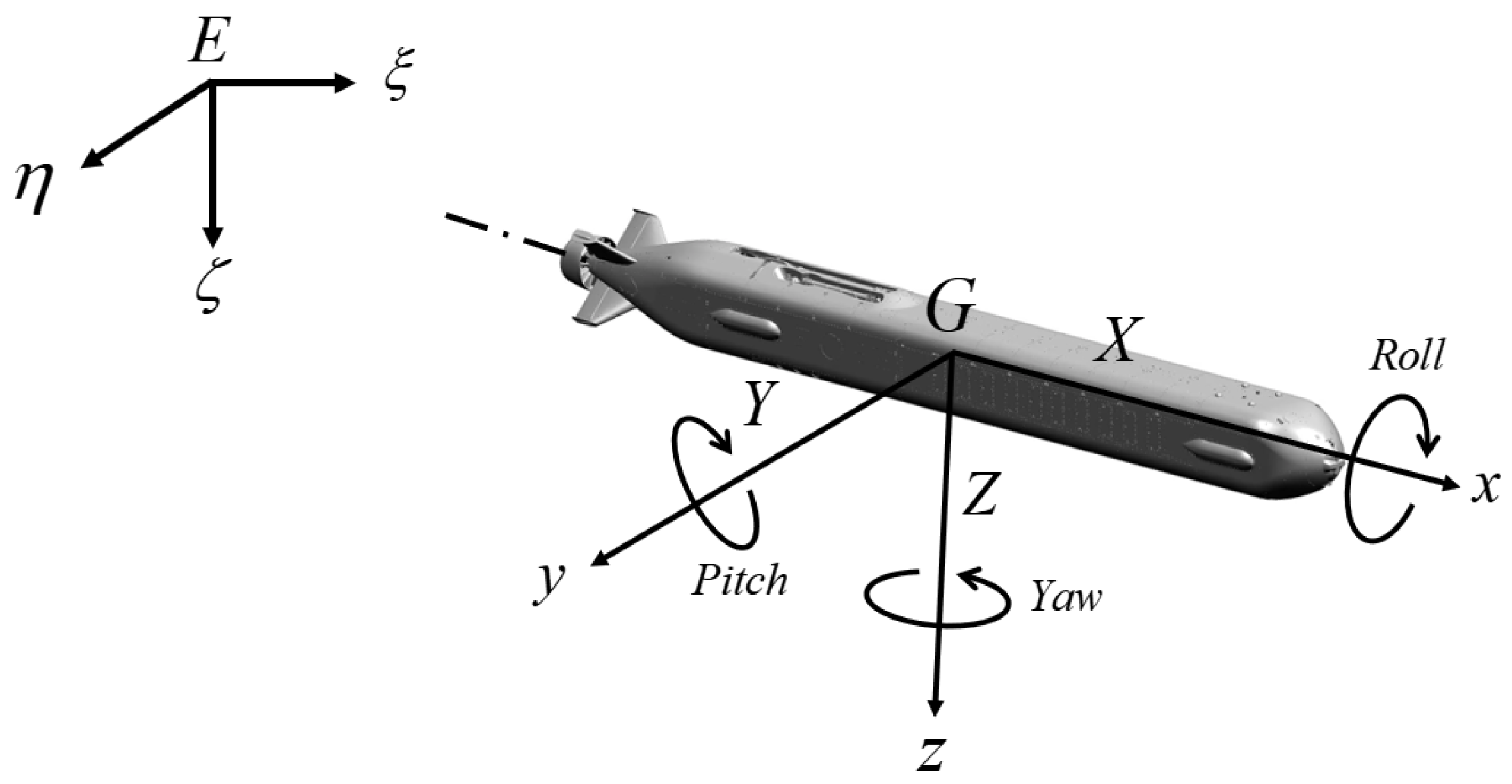
The corresponding coordinate system is the system of the Society of Naval and Marine Engineers (SNAME) [27] terminology bulletin recommended by the International Water Tank Conference (ITTC). The corresponding two right-handed Cartesian coordinate systems are shown in Figure 1. One is the fixed coordinate system $E-\xi \eta \zeta$, which is an inertial coordinate system used to represent the spatial position and attitude of LDUUV. The other is the motion coordinate system $G-xyz$, which is fixed to LDUUV and moves together with LDUUV. $E\xi$ is usually pointed to the main course of the LDUUV, $E\zeta$ points towards the center of the Earth, and $E\eta$ is vertical to $E-\xi \eta \zeta$. The origin G is usually set at the center of gravity of the LDUUV, with Gx, Gy, and Gz serving as the axial, lateral, and vertical directions of the LDUUV motion, respectively.

The motion of LDUUV has six degrees of freedom, including surge, sway, and heave, which refer to longitudinal, lateral, and vertical displacement, as well as yaw, roll, and pitch. Correspondingly, there are six independent coordinates to describe the position and attitude of the LDUUV. A geodetic coordinate system is defined for the six coordinates corresponding to the positions and directions along the x, y, and z axes, represented by $\left[x,y,z,\varphi ,\theta ,\psi \right]$. The influence of Earth’s rotation is ignored, since it is assumed that the fixed frame of the Earth is inertial. The linear and angular velocities $\left[u,v,w,p,q,r\right]$ are described in the fixed body coordinate system, which is a motion coordinate system with the origin fixed on the LDUUV.

2.2. Model Description and Uncertainty Analysis

The motion of LDUUV is affected by complex hydrodynamic forces, and these parameters (such as damping coefficient, additional mass coefficient, lift coefficient, etc.) are usually obtained through experiments or simulations; there are measurement errors or unmodeled dynamic effects. The uncertainty of LDUUV models is originally from various factors such as measurement errors in hydrodynamic parameters, disturbances in marine environments, nonlinearity of actuators, and unmodeled dynamics. These uncertainties can lead to low control accuracy, slower convergence speed, and even system instability. Therefore, the robustness and adaptability of controller design need to be fully considered, since they face dynamic changes and complex environmental disturbances.

LDUUV appearance and characteristics are similar to submarines; therefore, the mathematical model of LDUUV motion is established by investigating the nonlinear equation of the submarine control motion. LDUUV is regarded as a rigid body, applying the theory of center of mass motion and Euler dynamic equations to derive the translational and rotational equations of the LDUUV. The six degrees of freedom motion equations of the LDUUV are as follows:

$$\left\{\begin{array}{c}X=m\left[(\dot{u}-vr+wq)-x_G\left(q^2+r^2\right)+y_G(pr-\dot{r})+z_G(pr+\dot{q})\right]\hfill \\ Y=m\left[(\dot{v}-wp+ur)-y_G\left(r^2+p^2\right)+z_G(qr-\dot{p})+x_G(qp+\dot{r})\right]\hfill \\ Z=m\left[(\dot{w}-uq+vp)-z_G\left(p^2+q^2\right)+x_G(rp-\dot{q})+y_G(rq+\dot{p})\right]\hfill \\ K=I_{xx}\dot{p}+\left(I_{zz}-I_{yy}\right)qr+m\left[y_G(\dot{w}+pv-qu)-z_G(\dot{v}+ru-pw)\right]\hfill \\ M=I_{yy}\dot{q}+\left(I_{xx}-I_{zz}\right)rp+m\left[z_G(\dot{u}+qw-rv)-x_G(\dot{w}+pv-qu)\right]\hfill \\ N=I_{zz}\dot{r}+\left(I_{yy}-I_{xx}\right)pq+m\left[x_G(\dot{v}+ru-pw)-y_G(\dot{u}+qw-rv)\right]\hfill \end{array}\right.$$

(1)

The above equation represents the relationship between the external forces (X, Y, Z) and external moments (K, M, N), acting on the hull and the motion parameters when the center of mass does not coincide with the origin of the motion coordinate system. XG, YG, and ZG denote the position of the center of gravity of the LDUUV and serve as the reference centre of motion. The moments of inertia of the x-, y-, and z-axes, concerning the body-fixed coordinate system, are represented by Ixx, Iyy, and Izz, respectively, and the products of inertia satisfy the relationships Ixy = Iyx, Ixz = Izx, and Iyz = Izy.

Derive the dimensionless form of the six degree of freedom spatial motion equation of the X-rudder, when the center of gravity of the LDUUV coincides with the origin of the dynamic system, based on the submarine maneuverability equation and the forces and moments acting on the x-rudder LDUUV [28,29]. The origin of the dynamic system is taken at the center of gravity of the product; since xG = yG = zG = 0, Equation (1) can be rewritten as follows:

The axial force equation is

$$\begin{array}{c}m(\dot{u}-vr+wq)={\displaystyle \frac{1}{2}}\rho L^4\left[X_{qq}^{\prime }{q}^2+X_{rr}^{\prime }{r}^2+X_{rp}^{\prime }rp\right]\hfill \\ +{\displaystyle \frac{1}{2}}\rho L^3\left[X_u^{\prime }\dot{u}+X_{vr}^{\prime }vr+X_{wq}^{\prime }wq\right]+{\displaystyle \frac{1}{2}}\rho L^2\left[X_{uu}^{\prime }{u}^2+X_{vv}^{\prime }{v}^2+X_{ww}^{\prime }{w}^2\right]\hfill \\ +{\displaystyle \frac{1}{2}}\rho L^2\left[a_T{u}^2+b_{T}u{u}_c+c_T{u}_c^2\right]-(W-B)sin\theta +X_{\delta }\hfill \end{array}$$

(2)

The lateral force equation is

$$\begin{array}{c}m(\dot{v}-wp+ur)={\displaystyle \frac{1}{2}}\rho L^4\left[Y_r^{\prime }\dot{r}+Y_p^{\prime }\dot{p}+Y_{p\left|p\right|}^{\prime }p\left|p\right|+Y_{pq}^{\prime }pq+Y_{qr}^{\prime }qr+Y_{r\left|r\right|}^{\prime }r\left|r\right|\right]\hfill \\ +{\displaystyle \frac{1}{2}}\rho L^3\left[Y_{\dot{v}}^{\prime }\dot{v}+Y_r^{\prime }ur+Y_p^{\prime }up+Y_{vq}^{\prime }vq+Y_{wp}^{\prime }wp+Y_{wr}^{\prime }wr+Y_{v\left|r\right|}^{\prime }{\displaystyle \frac{v}{\left|v\right|}}\left|{\left(w^2+v^2\right)}^{{\displaystyle \frac{1}{2}}}\right|\left|r\right|\right]\hfill \\ +{\displaystyle \frac{1}{2}}\rho L^2\left[Y_0^{\prime }{u}^2+Y_v^{\prime }uv+Y_{v\left|v\right|}^{\prime }v\left|{\left(w^2+v^2\right)}^{{\displaystyle \frac{1}{2}}}\right|+Y_{vv}^{\prime }vw\right]+(W-B)cos\theta sin\varphi +Y_{\delta }\hfill \end{array}$$

(3)

The vertical force equation is

$$\begin{array}{c}m(\dot{w}-uq+vp)={\displaystyle \frac{1}{2}}\rho L^4\left[Z_{\dot{q}}^{\prime }\dot{q}+Z_{pp}^{\prime }{p}^2+Z_{rr}^{\prime }{r}^2+Z_{rp}^{\prime }rp+Z_{q\left|q\right|}^{\prime }q\left|q\right|\right]\hfill \\ +{\displaystyle \frac{1}{2}}\rho L^3\left[Z_{\dot{w}}^{\prime }\dot{w}+Z_q^{\prime }uq+Z_{vr}^{\prime }vr+Z_{vp}^{\prime }vp+Z_{w\left|q\right|}^{\prime }{\displaystyle \frac{w}{\left|w\right|}}\left|{\left(v^2+w^2\right)}^{{\displaystyle \frac{1}{2}}}\right|\left|q\right|\right]\hfill \\ +{\displaystyle \frac{1}{2}}\rho L^2\left[Z_0^{\prime }{u}^2+Z_w^{\prime }uw+Z_{\left|w\right|}^{\prime }u\left|w\right|+Z_{ww}^{\prime }\left|w{\left(v^2+w^2\right)}^{{\displaystyle \frac{1}{2}}}\right|\right]\hfill \\ +{\displaystyle \frac{1}{2}}\rho L^2\left[Z_{w\left|w\right|}^{\prime }w\left|{\left(v^2+w^2\right)}^{{\displaystyle \frac{1}{2}}}\right|+Z_{vv}^{\prime }{v}^2\right]+(W-B)cos\theta cos\varphi +Z_{\delta }\hfill \end{array}$$

(4)

The roll moment equation is

$$\begin{array}{c}{I}_x\dot{p}+\left(I_z-I_y\right)qr={\displaystyle \frac{1}{2}}\rho L^5\left[K_{\dot{p}}^{\prime }\dot{p}+K_{\dot{r}}^{\prime }\dot{r}+K_{p\left|p\right|}^{\prime }p\left|p\right|+K_{qr}^{\prime }qr+K_{pq}^{\prime }pq+K_{r\left|r\right|}^{\prime }r\left|r\right|\right]\hfill \\ +{\displaystyle \frac{1}{2}}\rho L^4\left[K_{\dot{v}}^{\prime }\dot{v}+K_p^{\prime }up+K_r^{\prime }ur+K_{vq}^{\prime }vq+K_{wp}^{\prime }wp+K_{wr}^{\prime }wr\right]\hfill \\ +{\displaystyle \frac{1}{2}}\rho L^3\left[K_0^{\prime }{u}^2+K_v^{\prime }uv+K_{v\left|v\right|}^{\prime }v\left|{\left(v^2+w^2\right)}^{{\displaystyle \frac{1}{2}}}\right|+K_{vw}^{\prime }vw\right]\hfill \\ -\left(z_{G}W-z_{C}B\right)cos\theta sin\varphi +K_{\delta }\hfill \end{array}$$

(5)

The pitch moment equation is

$$\begin{array}{c}{I}_y\dot{q}+\left(I_x-I_z\right)rp={\displaystyle \frac{1}{2}}\rho L^5\left[M_{\dot{q}}^{\prime }\dot{q}+M_{pp}^{\prime }{p}^2+M_{q\left|q\right|}^{\prime }q\left|q\right|+M_{rr}^{\prime }{r}^2+M_{rp}^{\prime }rp\right]\hfill \\ +{\displaystyle \frac{1}{2}}\rho L^4\left[M_{\dot{w}}^{\prime }\dot{w}+M_q^{\prime }uq+M_{vr}^{\prime }vr+M_{vp}^{\prime }vp+M_{\left|w\right|q}^{\prime }\left|{\left(v^2+w^2\right)}^{{\displaystyle \frac{1}{2}}}\right|q\right]\hfill \\ +{\displaystyle \frac{1}{2}}\rho L^3\left[M_0^{\prime }{u}^2+M_w^{\prime }uw+M_{\left|w\right|}^{\prime }u\left|w\right|+M_{w\left|w\right|}^{\prime }w\left|{\left(v^2+w^2\right)}^{{\displaystyle \frac{1}{2}}}\right|\right]\hfill \\ +{\displaystyle \frac{1}{2}}\rho L^3\left[M_{ww}^{\prime }\left|w{\left(v^2+w^2\right)}^{{\displaystyle \frac{1}{2}}}\right|+M_{vv}^{\prime }{v}^2\right]-\left(z_{G}W-z_{C}B\right)sin\theta +M_{\delta }\hfill \end{array}$$

(6)

The yaw moment equation is

$$\begin{array}{c}{I}_z\dot{r}+\left(I_y-I_x\right)pq={\displaystyle \frac{1}{2}}\rho L^5\left[N_{\dot{r}}^{\prime }\dot{r}+N_{\dot{p}}^{\prime }\dot{p}+N_{p\left|p\right|}^{\prime }p\left|p\right|+N_{r\left|r\right|}^{\prime }r\left|r\right|+N_{pq}^{\prime }pq+N_{qr}^{\prime }qr\right]\hfill \\ +{\displaystyle \frac{1}{2}}\rho L^4\left[N_{\dot{v}}^{\prime }\dot{v}+N_p^{\prime }up+N_r^{\prime }ur+N_{wr}^{\prime }wr+N_{wp}^{\prime }wp+N_{vq}^{\prime }vq+N_{\left|p\right|r}^{\prime }\left|{\left(v^2+w^2\right)}^{{\displaystyle \frac{1}{2}}}\right|r\right]\hfill \\ +{\displaystyle \frac{1}{2}}\rho L^3\left[N_0^{\prime }{u}^2+N_v^{\prime }uv+N_{v\left|v\right|v}^{\prime }v\left|{\left(v^2+w^2\right)}^{{\displaystyle \frac{1}{2}}}\right|+N_{vw}^{\prime }vw\right]+N_{\delta }\hfill \end{array}$$

(7)

The rudders force in the external force (moment) acting on the spatial motion of the x-rudder vehicle can be calculated by the following equation [1]:

$$\begin{array}{c}{X}_{\delta }=X_{{\delta }_1}{u}^2\left|{\delta }_1\right|+X_{{\delta }_2}{u}^2\left|{\delta }_2\right|+X_{{\delta }_3}{u}^2\left|{\delta }_3\right|+X_{{\delta }_4}{u}^2\left|{\delta }_4\right|\hfill \\ Y_{\delta }=Y_{{\delta }_1}{u}^2{\delta }_1+Y_{{\delta }_2}{u}^2{\delta }_2+Y_{{\delta }_3}{u}^2{\delta }_3+Y_{{\delta }_4}{u}^2{\delta }_4\hfill \\ Z_{\delta }=Z_{{\delta }_1}{u}^2{\delta }_1+Z_{{\delta }_2}{u}^2{\delta }_2+Z_{{\delta }_3}{u}^2{\delta }_3+Z_{{\delta }_4}{u}^2{\delta }_4\hfill \\ K_{\delta }=K_{{\delta }_1}{u}^2{\delta }_1+K_{{\delta }_2}{u}^2{\delta }_2+K_{{\delta }_3}{u}^2{\delta }_3+K_{{\delta }_4}{u}^2{\delta }_4\hfill \\ M_{\delta }=M_{{\delta }_1}{u}^2{\delta }_1+M_{{\delta }_2}{u}^2{\delta }_2+M_{{\delta }_3}{u}^2{\delta }_3+M_{{\delta }_4}{u}^2{\delta }_4\hfill \\ N_{\delta }=N_{{\delta }_1}{u}^2{\delta }_1+N_{{\delta }_2}{u}^2{\delta }_2+N_{{\delta }_3}{u}^2{\delta }_3+N_{{\delta }_4}{u}^2{\delta }_4\hfill \end{array}$$

(8)

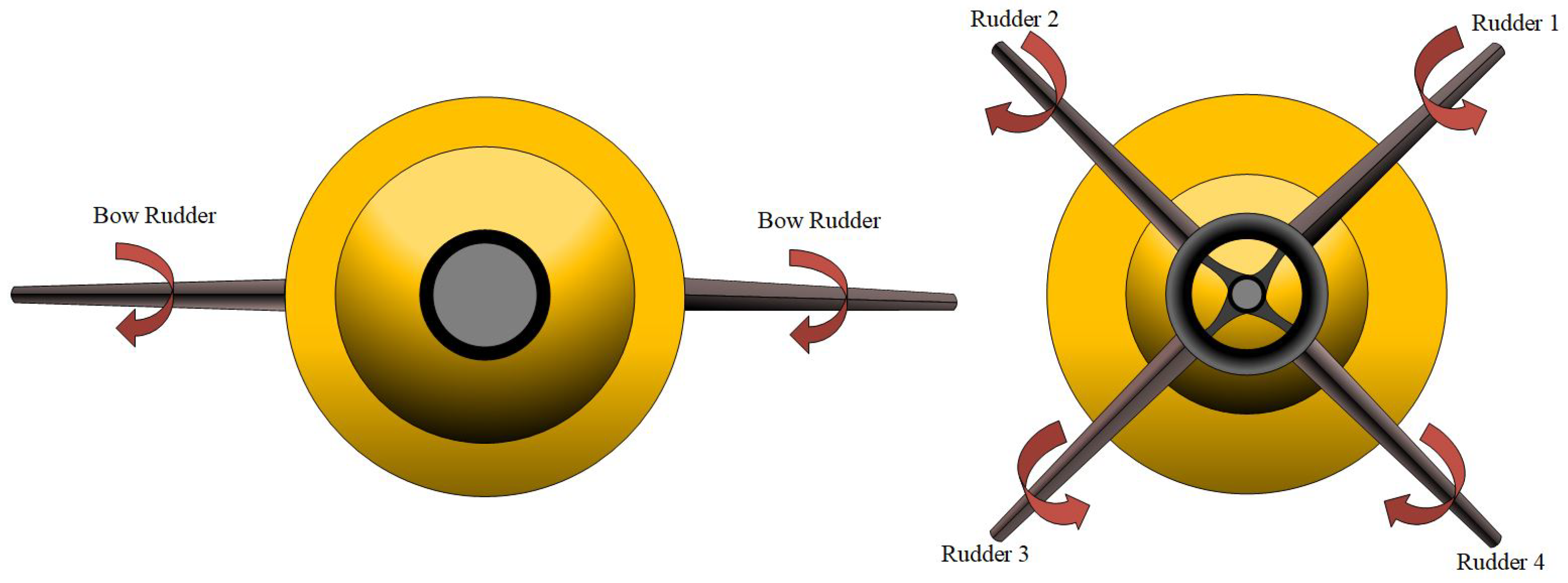
In Figure 2, the stern x-shaped rudder configuration is shown on the right, while the bow rudder configuration is shown on the left. The x-rudder and cross-rudder are suitable for different AUV control requirements. The design of a cross-rudder consists of two mutually perpendicular control surfaces, located in the vertical and horizontal planes, respectively. The horizontal rudder is responsible for pitch control, thereby adjusting the ascent and descent of the LDUUV. The vertical rudder is responsible for heading control and is used to change the left and right direction. The layout of the x-rudder is obtained by deflecting the rudder surface 45° along the central axis of the hull based on the cross-rudder. Four control surfaces are distributed in an x-shaped layout; each control surface of the x-rudder affects pitch and heading simultaneously. The main advantage of the x-rudder is that it increases maneuverability, especially in complex underwater navigation, with good stability and agility.

2.3. Analysis of Motion Equations for Horizontal Plane

In the study of decoupling horizontal subsystems, roll motion is usually ignored to reduce the complexity of the problem, so only lateral velocity v, heading angular velocity r, and forward velocity u are considered. If it is assumed that the forward speed u can be kept stable by a forward speed controller, which will simultaneously compensate for the interference of motion on u due to other axes, then the forward speed u can be eliminated from the longitudinal motion equation. Assuming that the center of gravity coincides with the origin of the inertial frame on the horizontal plane, the model can be further simplified to derive the dynamic model of the horizontal subsystem. The vertical face system can also be simplified using the following equations.

Usually, in the design of complex dynamic controllers, to facilitate the design, the six degrees of freedom dynamic model is often decoupled as a three degrees of freedom model. This paper decouples the dynamic model of LDUUV into a horizontal motion model and a vertical motion model for a large inertia underwater robot equipped with bow rudder and x-shapes stern rudder, ignoring its roll direction motion. The horizontal plane dynamic model is as follows:

$$\left\{\begin{array}{c}m(\dot{u}-vr)=X_{\dot{u}}\dot{u}+X_{uu}{u}^2+X_{vv}{v}^2+X_{rr}{r}^2+X_{vv}v{r}^2+X_{\delta \dot{\delta }}{\delta }^2+X_T\hfill \\ m(\dot{v}+ur)=Y_{\dot{v}}\dot{v}+Y_{\dot{r}}\dot{r}+Y_{v}v+Y_{r}r+Y_{v\left|v\right|}v\left|v\right|+Y_{r\left|r\right|r\mid }r\left|r\right|+Y_{v\left|r\right|r}v\left|r\right|\hfill \\ +Y_{\delta }\delta +Y_{\left|r\right|\delta }\left|r\right|\delta \hfill \\ I_z\dot{r}=N_{\dot{v}}\dot{v}+N_{\dot{r}}\dot{r}+N_{v}v+N_{r}r+N_{v\left|v\right|}v\left|v\right|+N_{v\left|r\right|}v\left|r\right|+N_{r\left|r\right|}r\left|r\right|+N_{\delta }\delta \hfill \\ +N_{\left|r\right|\delta }\left|r\right|\delta \hfill \end{array}\right.$$

(9)

where m is the mass; $X_{\dot{u}},X_{uu},X_{vv},Y_{\dot{v}},Y_{\dot{r}},Y_{v\left|r\right|},N_{\dot{v}},N_{\dot{r}},N_v$ denote the hydrodynamics coefficients of surge, sway, and yaw direction respectively; $I_z$ is the inertial tensor about z-axis; $X_T$ is the propeller thrust in the forward direction; $X_{\delta \delta },{\delta }^2{Y}_{\delta }\delta +Y_{\left|r\right|\delta }\left|r\right|\delta ]$ and $N_{\delta }\delta +N_{\left|r\right|\delta }\left|r\right|\delta$ are the force generated by the rudder of the surge, sway, and yaw direction respectively. The forces and moments generated by the rudders are given by Equation (8).

To facilitate the design of the control law, Equation (9) is simplified as

$$\left\{\begin{array}{c}\dot{u}={\alpha }_u+{\beta }_u{X}_T\hfill \\ \dot{v}={\alpha }_v+{\beta }_v{X}_T\hfill \\ \dot{r}={\alpha }_r+{\beta }_r{\tau }_r\hfill \end{array}\right.$$

(10)

where

$$\begin{array}{c}{\alpha }_u=X_{uu}{u}^2+X_{vv}{v}^2+X_{rr}{r}^2+X_{vr}v{r}^2-mvr\hfill \\ {\beta }_u=1/m-X_{\dot{u}}\hfill \\ {\tau }_u=X_{\delta \delta }{\delta }^2\hfill \\ {\tau }_T=X_T\hfill \\ {\alpha }_v=Y_{\dot{r}}\dot{r}+Y_{v}v+Y_{r}r+Y_{v\left|v\right|}v\left|v\right|+Y_{r\left|r\right|r}r\left|r\right|+Y_{v\left|r\right|}v\left|r\right|-mur\hfill \\ {\beta }_v=1/m-Y_{\dot{v}}\hfill \\ {\tau }_v=Y_{\delta }\delta +Y_{\left|r\right|\delta }\left|r\right|\delta \hfill \\ {\alpha }_r=Y{N}_{\dot{v}}\dot{v}++N_{v}v+N_{r}r+N_{v\left|v\right|}v\left|v\right|+N_{v\left|r\right|}v\left|r\right|+N_{r\left|r\right|}r\left|r\right|\hfill \\ {\beta }_r=I_z-N_{\dot{r}}\hfill \\ {\tau }_r=N_{\delta }\delta +N_{\left|r\right|\delta }\left|r\right|\delta \hfill \end{array}$$

(11)

3. Controller Design

In this section, the cascaded controller is designed for the control of basic movements such as heading. In traditional sliding mode control methods, external disturbances, model uncertainty, and actuator saturation are not considered. When the underwater vehicle model and hydrodynamic coefficients are unknown and model-based methods are not applicable, a model-free fast terminal sliding mode control framework based on reinforcement learning is introduced. This approach adaptively tunes controller parameters in real time to ensure robust and accurate dynamic control under uncertainty.

3.1. Sliding Mode Controller Design

Sliding mode control is a commonly used method in control systems, which has been widely used in underwater robot control due to its robustness to external disturbances and model uncertainties.

To derive the control law, the heading error is defined as ${\psi }_e=\psi -{\psi }_r$, and the sliding surface is given as

$$s={\dot{\psi }}_e+{\alpha }_0{\psi }_e$$

(12)

By analyzing Equation (10), the second-order derivative of course can be derived as

$$\ddot{\psi }=\dot{r}={\alpha }_r+{\beta }_r{\tau }_r$$

(13)

The goal of sliding surface design is to enable the state of the control system to approach zero along the sliding surface, ensuring that the system error converges to zero. In this sliding surface function, several different error terms are included to optimize different response characteristics:

(1)

${\psi }_e$ represents the derivative of the error, reflecting the rate of the error ny adjusting to control the rapid response of the system to errors.

(2)

${\alpha }_0{\psi }_e$ represents the current error term, which directly affects the steady-state accuracy of the system. By increasing the value of ${\psi }_e$, the sensitivity of the sliding mode to the error will be enhanced, which helps to converge the error to zero faster.

To derive the control law, a Lyapunov candidate is selected as

$$V={\displaystyle \frac{1}{2}}{s}^2$$

(14)

By analyzing Equation (14), its derivative can be derived as

$$\dot{V}=s\dot{s}$$

(15)

Multiplying Equations (12) and (15), Equation (15) can be represented as follows:

$$\begin{array}{cc}\hfill \dot{V}& =s\dot{s}=\left({\dot{\psi }}_e+{\alpha }_0{\psi }_e\right)\left({\ddot{\psi }}_e+{\alpha }_0{\dot{\psi }}_e\right)\hfill \\ \hfill & =\left({\dot{\psi }}_e+{\alpha }_0{\psi }_e\right)\left(\ddot{\psi }-{\ddot{\psi }}_r+{\alpha }_0{\dot{\psi }}_e\right)\hfill \\ \hfill & =\left({\dot{\psi }}_e+{\alpha }_0{\psi }_e\right)\left({\alpha }_r+{\beta }_r{\tau }_r-{\ddot{\psi }}_r+{\alpha }_0{\dot{\psi }}_e\right)\hfill \end{array}$$

(16)

Based on the Lyapunov stability theory, the stability of the control system is usually guaranteed by constructing a positive definite Lyapunov function $V\left(x\right)$. Analyze $V\left(x\right)$ and ensure its derivative $\dot{V}\left(x\right)$ is non-positive definite, within the entire system state space.

Inspired by the tuning philosophy in [1], the proportional gain $k_1$ is designed to ensure rapid convergence of the sliding surface, and the nonlinear gain $k_2$ is configured to suppress disturbances and model uncertainties while minimizing chattering effects. Subsequently, these parameters were fine-tuned through simulation studies to adapt to the dynamic characteristics of our specific system. This two-step process—starting from a theoretically grounded baseline and then refining through practical validation—ensured both stability and performance in real-time implementation. For the above sliding surface design, the course control law is designed as:

$${\tau }_r={\displaystyle \frac{1}{{\beta }_r}}({\ddot{\psi }}_r-{\alpha }_r-{\alpha }_0{\dot{\psi }}_e-k_{1}s-k_{2}tanh\left(s\right))$$

(17)

where $k_1$ is the proportional gain of sliding mode control; $k_2$ is the nonlinear gain of sliding mode control.

The parameters taken by the traditional sliding mode controller in this paper are defined as follows: ${\alpha }_0=0.05$; $k_1=2.35$; $k_2=0.05$.

For further stability analysis, Equation (14) is substituted into Equation (16), from which the derivative of the Lyapunov function is obtained as

$$\dot{V}=s(-k_{1}s-k_{2}tanh\left(s\right))$$

(18)

Due to the uniqueness of the nonlinear functions $tanh\left(s\right)$, which approximates linearly around $s\to 0$ and rapidly approaches a constant, this control law has the characteristics of fast convergence and suppression of chattering.

As an odd function, $tanh\left(s\right)$ satisfies $tanh(-s)=-tanh\left(s\right)$, with range $[-1,1]$. The specific analysis of whether the derivative of V conforms to Lyapunov stability is as follows:

(1)

If $s>0$ or $s<0$, $-k_1{s}^2<0$;

(2)

If $s>0$, $tanh\left(s\right)>0$, $-k_{2}stanh\left(s\right)<0$;

(3)

If $s<0$, $tanh\left(s\right)<0$, $-k_{2}stanh\left(s\right)<0$.

Since $\dot{V}\le 0$ for all s, and $\dot{V}<0$ whenever $s\ne 0$, it can be concluded from Lyapunov’s direct method that the equilibrium at $s=0$ is globally asymptotically stable.

3.2. Design of Sliding Mode Controller Based on Reinforcement Learning

3.2.1. Design of Fast Terminal Sliding Mode Controller

A nonlinear sliding surface is introduced by the fast terminal sliding mode controller, which can enable the system to converge within a finite time. This terminal sliding surface design can ensure the rapid attainment of a stable state of the system without requiring a deep understanding of the global dynamic characteristics of the system. This feature enables fast terminal sliding mode control to exhibit certain “model independent” characteristics in some situations, making it suitable for nonlinear and highly uncertain systems. This method can effectively reduce the dependence on the system model when facing unknown or uncertain dynamic systems.

To derive the control law, the heading error is defined as ${\psi }_e={\psi }_r-\psi$, and the sliding surface is given as

$$s={\dot{\psi }}_e+{\alpha }_1{{\psi }_e}^p+\beta {{\psi }_e}^q$$

(19)

where ${\psi }_e$ represents the current error term; ${\alpha }_1\beta$ are the proportionality coefficients of the sliding surface.

For the above sliding surface design, the course control law is designed as

$$u=-k_{3}s-k_4{\left|s\right|}^{\gamma }tanh\left(s\right)$$

(20)

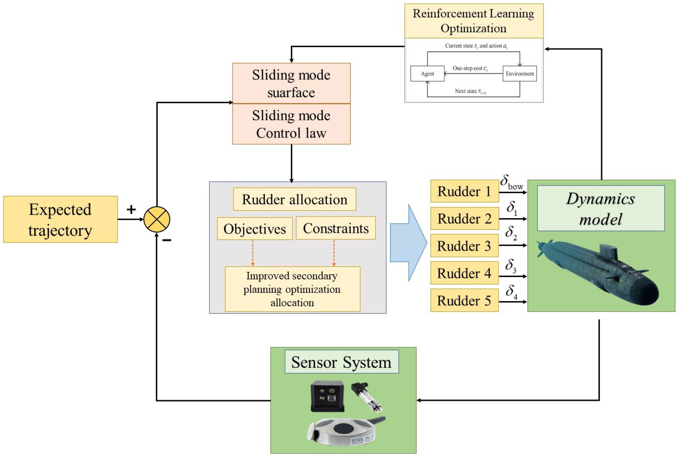
As illustrated in Figure 3, the proposed control framework integrates sliding mode controller, reinforcement learning optimization, and x-rudder allocation.

3.2.2. Analysis of Lyapunov Stability

To guarantee the stability of the control system, a Lyapunov candidate is selected as

$$V={\displaystyle \frac{1}{2}}{s}^2$$

(21)

By analyzing Equation (21), its derivative can be derived as

$$\dot{V}=s\dot{s}$$

(22)

Multiplying Equations (19) and (22), Equation (22) can be derived as follows:

$$\dot{V}=s\dot{s}=s({\ddot{\psi }}_e+{\alpha }_{1}p{{\psi }_e}^{p-1}{\dot{\psi }}_e+\beta q{{\psi }_e}^{q-1}{\dot{\psi }}_e)$$

(23)

The error dynamic equation of the system is $\ddot{x}=u+f(x,\dot{x})$. Therefore, the second-order derivative of course error can be derived as

$${\ddot{\psi }}_e=\ddot{\psi }-{\ddot{\psi }}_d=u+f({\psi }_e,{\ddot{\psi }}_e)$$

(24)

Substituting Equation (20) into Equation (24), Equation (24) can be rewritten as

$${\ddot{\psi }}_e=-k_{3}s-k_4{\left|s\right|}^{\gamma }tanh\left(s\right)+f({\psi }_e,{\ddot{\psi }}_e)$$

(25)

By substituting Equation (25) into Equation (23), Equation (23) can be derived as follows:

$$\dot{V}=s(-k_{3}s-k_4{\left|s\right|}^{\gamma }tanh\left(s\right)+f({\psi }_e,{\ddot{\psi }}_e)+{\alpha }_{1}p{{\psi }_e}^{p-1}{\dot{\psi }}_e+\beta q{{\psi }_e}^{q-1}{\dot{\psi }}_e)$$

(26)

The influence of nonlinear term $f({\psi }_e,{\ddot{\psi }}_e)$ can be eliminated through compensation methods or learning strategies (or assuming that this term can be ignored).

The specific stability analysis process is listed as follows:

(1)

$-k_3{s}^2\le 0$, ${\left|s\right|}^{\gamma }>0$, $-k_{4}s{\left|s\right|}^{\gamma }tanh\left(s\right)<0$;

(2)

For the unknown nonlinear term $sf({\psi }_e$, ${\ddot{\psi }}_e)$, which can be assumed to be ignored;

(3)

If ${\psi }_e\to 0$, ${{\psi }_e}^{p-1}\to 0$, ${{\psi }_e}^{q-1}\to 0$.

The design of the sliding surface can control the effect of this factor within an effective range.

According to the above analysis, the derivative of the Lyapunov function satisfies:

$$\dot{V}\le -k_3{s}^2-k_4|s{|}^{\gamma +1}+\epsilon$$

(27)

where $\epsilon$ represents the residual effects of the third and fourth terms. When the controller gains $k_3$ and $k_4$ are large enough, they can be ignored. Therefore, Equation (27) can be rewritten as

$$\dot{V}\le -k_3{s}^2-k_4|s{|}^{\gamma +1}$$

(28)

The faster growth rate of $|s{|}^{\gamma +1}$ compared to $s^2$ ($0<\gamma <1$) ensures that the sliding surface $s\to 0$ is within finite time. Therefore, $\dot{V}\le 0$ is guaranteed.

3.3. Optimization of Sliding Mode Parameters Based on Reinforcement Learning

Controller design involves various parameters ${\alpha }_1,\beta ,k3,k4,p,q,\gamma$. Conventional methods for tuning sliding mode controllers often require repeated manual adjustments of the controller parameters, whereas reinforcement learning enables their automatic optimization. Due to the large number of control variables, we fix the control parameters of the sliding surface and only need to train the parameters of the controller.

Therefore, the obtained fixed parameters are ${\alpha }_1=0.05,\beta =0.02,p=2.0,q=0.5$.

The specific design of the reinforcement learning control process is as follows:

(1)

State and Action Design:

States: System input states error $\left[{\psi }_e,{\dot{\psi }}_e\right]$;

Action: Controller output parameters $k3,k4,\gamma$.

(2)

Reward function design:

The design of the reward function is as follows, and the specific hierarchical reinforcement learning reward function is shown in Algorithm 1:

$$\mathrm{Reward}=tanh\left(k11\ast abs\left(e_{\_}\mathrm{depth}\right)+k12\ast w+k13\ast r+k14\ast abs\left(e_{\_}\mathrm{pesi}\right)\right)$$

(29)

where $k11=-0.01,k12=-0.02,k13=-0.05,k14=-0.05$, $e_{\_}\mathrm{depth}$ is the error of depth, and $e_{\_}\mathrm{pesi}$ is the error of the course.

The goal of RL is to maximize long-term returns by optimizing current behaviors, enabling agents to make optimal decisions in each state. The DDPG algorithm is used to solve continuous action space problems, combining the ideas of deterministic strategies and empirical replay [12]. By designing a reasonable strategy network, oscillations and instability during the training process can be reduced, and parameters can be dynamically adjusted based on current state feedback to enhance the dynamic performance of the controller.

The Markov Decision Process (MDP) is defined by the tuple $\mathcal{M}=(\mathcal{S},\mathcal{A},\mathcal{P},r,\gamma )$, where $\mathcal{S}$ is the state space, $\mathcal{A}$ is the action space, $\mathcal{P}\left(s^{\prime }\right|s,a)$ denotes the state transition probability, $r(s,a)$ is the reward function, and $\gamma \in (0,1)$ is the discount factor. The cumulative discounted reward (also called the return) starting from time step t is defined as:

$$R_t=\sum _{k=0}^{\infty }{\gamma }^k{r}_{t+k}$$

(30)

To evaluate the quality of a state or a state–action pair under a given policy $\pi$, RL defines two fundamental value functions: the state-value function and the action-value function, also known as the Q-function. The state-value function $V^{\pi }\left(s\right)$ represents the expected cumulative discounted reward that the agent can obtain starting from state s and thereafter following policy $\pi$:

$$V^{\pi }\left(s\right)=\mathbb{E}\left[\sum _{t=0}^{\infty }{\gamma }^t{r}_t\mid s_0=s\right]$$

(31)

The action-value function $Q^{\pi }(s,a)$ is defined as the expected cumulative discounted reward when the agent starts from state s, takes action a, and subsequently follows the policy $\pi$ for all future steps.

$$Q(s,a)=\mathbb{E}\left[\sum _{t=0}^{\infty }{\gamma }^t{r}_t\mid s_0=s,a_0=a\right]$$

(32)

where r is the immediate reward obtained at time step t; $\gamma$ is the discount factor used to attenuate the impact of future rewards; s and a are the state and action, respectively.

In the actor–critic architecture, such as in the DDPG algorithm, the critic network is trained to approximate the action-value function $Q^{\pi }(s,a)$ using sampled interactions, while the actor-network is updated to select actions that maximize this Q-value. This enables the agent to iteratively improve its policy in continuous action spaces.

The critic network of DDPG updates Q-values through the Bellman equation, which can be repressed as follows:

$$y=r+\gamma Q^{\prime }\left(s^{\prime },a^{\prime };{\theta }^{\prime }\right)$$

(33)

where r is the immediate reward; s is the next state and a is action; $\gamma$ is the discount factor; $\theta$ is the parameter of the target network.

The goal of the critic network is to update the parameters of the Q-value network by minimizing the following loss function, which is given as follows:

$$L\left(\theta \right)=\mathrm{E}\left[{(y-Q(s,a;\theta \left)\right)}^2\right]$$

(34)

The update of the actor utilizes the policy gradient method to maximize the Q-value through gradient ascent. The update process of the actor-network can be represented as follows:

$${\nabla }_{{\theta }^{\mu }}J\approx \mathrm{E}\left[{\nabla }_{a}Q\left(s,a;{\theta }^Q\right){\nabla }_{{\theta }^{\mu }}\mu \left(s;{\theta }^{\mu }\right)\right]$$

(35)

where J is the objective function of the actor-network; $\mu \left(s;{\theta }^{\mu }\right)$ is the output action of the actor-network; $\theta$ is the parameter of the actor-network; $Q\left(s,a;{\theta }^Q\right)$ is the output of the critic network; ${\theta }^Q$ is the parameter of the critic network.

In order to dynamically adjust the parameters of the sliding mode controller in real time, $k3$, $k4$, and $\gamma$ are selected as the tuning parameters for the proposed control algorithm. The parameter optimization algorithm for sliding mode control based on reinforcement learning proposed in this paper is shown in Algorithm 1.

Algorithm 1 Implementation of parameter optimization control algorithm

1: Initialize environment and proxy model; 2: Extract ObservationInfo and ActionInfo; 3: Custom Cache ReplayBuffer; 4: Create an intelligent agent network setup DDPGNetworks and set training parameters; For episode = 1:numEpisodes  5: Reset environment state parameters;  6: Initialize variables used to store data for this round;  For step = 1:maxSteps   7: Intelligent agent generates actions;   If $i_{cnt}>=10$, obtain the action generated by reinforcement learning every 10 steps;   8: The sliding mode control parameters k3, k4, and r obtained through DDPG training are inputted into the controller, and the optimized control parameters are input into the horizontal rudder angle dr and vertical rudder angle de;   9: Control allocation of bow and stern rudder through improved quadratic planning rudder command allocation method;   10: Reward function setting:    $Reward=tanh\left(k11\ast abs\left(e_{\_}\mathrm{depth}\right)+k12\ast w+k13\ast r+k14\ast abs\left(e_{\_}\mathrm{pesi}\right)\right)$;    If $abs\left(e_{\_}\mathrm{depth}\right)<0.1$     $Reward=Reward+0.05$;    end    If $abs\left(e_{\_}\mathrm{pesi}\right)<1\ast D2R$     $Reward=Reward+0.1$;    end    If $abs\left(e_{\_}\mathrm{pesi}\right)>10$     $Reward=Reward-4\ast abs\left(e_{\_}\mathrm{pesi}\right)$;    end    If $abs\left(e_{\_}\mathrm{pesi}\right)<5\ast D2R$     $Reward=Reward+2\ast (5\ast D2R-abs\left(e_{\_}\mathrm{pesi}\right))$;    end    If $abs\left(e_{\_}\mathrm{pesi}\right)<0.1\ast D2R$     $stabl{e}_{\_}\mathrm{time}=stabl{e}_{\_}\mathrm{time}+1$;    If $stabl{e}_{\_}\mathrm{time}>=1000$     $IsDone=true$;    end    else     $stabl{e}_{\_}\mathrm{time}=0$;    end   11: Storage Experience to ReplayBuffer;   12: Update the current state to state = NextState;   13: Save relevant data such as status, actions, and rewards;   14: Check if the termination conditions have been met.  end end

Compared with the traditional fixed gain sliding mode controller, the reinforcement learning-based sliding mode controller can adaptively adjust control gains in response to dynamic disturbances. This enhances the system’s robustness to model uncertainties and environmental interferences, as validated by the Lyapunov analysis and simulation results. The sliding controller parameters are optimized by the DDPG algorithm, with the sliding surface converging within a finite time while avoiding chattering. Algorithm 1 utilizes the DDPG framework to adaptively tune the nonlinear sliding mode parameters in a continuous control space. 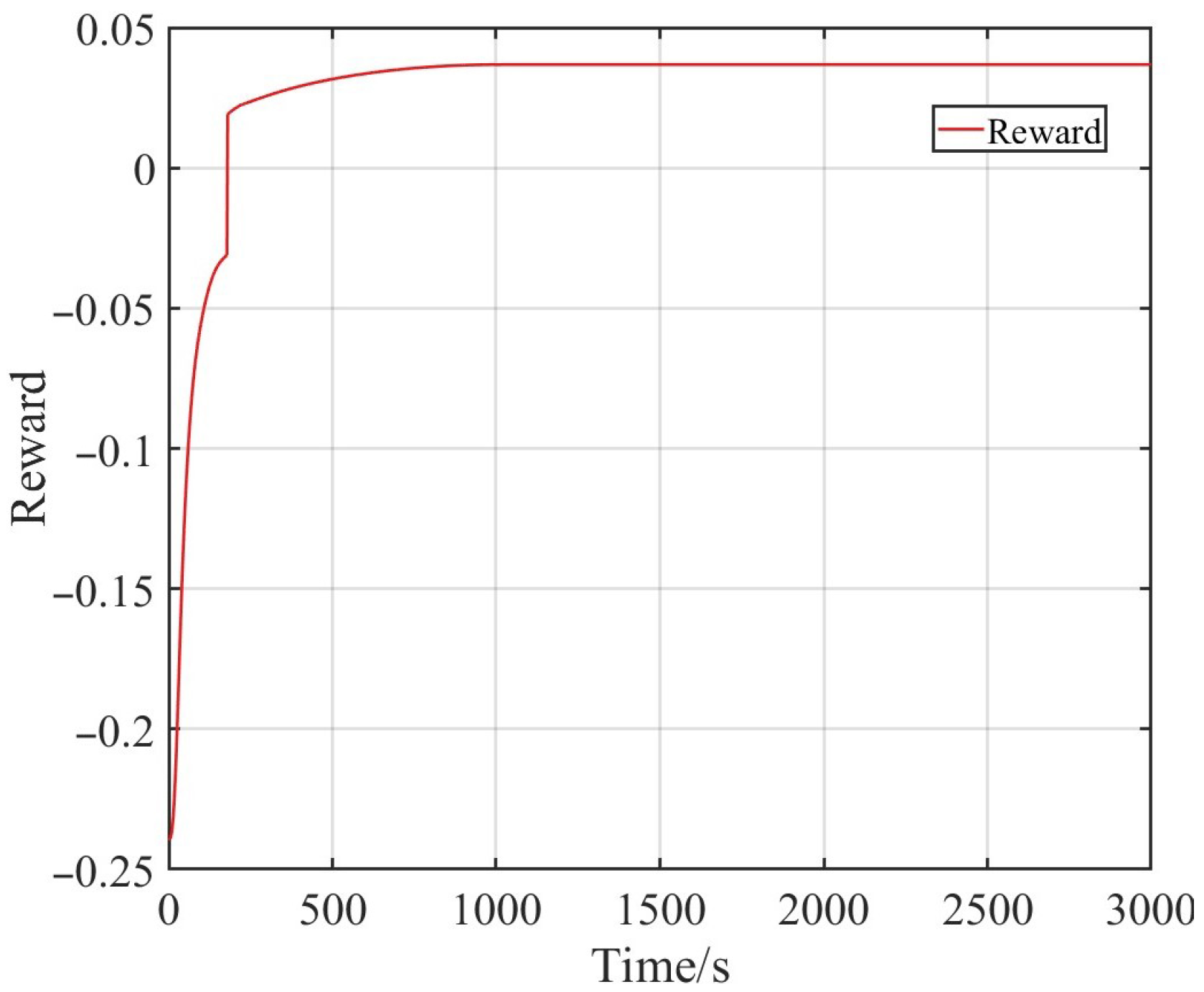Only a subset of parameters $k3,k4,\gamma$ are selected to reduce learning complexity while ensuring sufficient performance improvement. This strategy strikes a balance between control effectiveness and training convergence, as illustrated by the stable reward curve in Figure 4.

3.4. Improved Secondary Planning Rudder Command Allocation

A modified quadratic programming algorithm is proposed for the control allocation problem, while considering actuator constraints and objective optimization. The method of optimizing control allocation for each of the five rudder commands can be shown as follows:

(1)

Establish an action matrix based on the rudder layout of the AUV:

$${\mathbf{T}}_{\mathbf{actual}}=\mathbf{H}\mathbf{\delta }$$

(36)

where ${\mathbf{T}}_{\mathbf{actual}}={\left[F_x,F_y,F_z,M_x,M_y,M_z\right]}^{\mathsf{T}}$, the total force and torque actually generated by rudder commands; $\mathbf{H}$ represents the matrix of rudder allocation, which includes the installation position and operational efficiency of the rudder; $\delta$ represents the vector of the rudder angle.

(2)

The optimization goal is to minimize the error (the difference between the desired torque and the actual torque) and the energy consumption. The optimization method is designed as

$$\underset{\delta }{min}{∥{\mathbf{T}}_{\mathbf{cmd}}-\mathbf{H}\mathbf{\delta }∥}^2+\lambda {∥\delta -{\delta }_{\mathrm{prev}}∥}^2$$

(37)

where ${\mathbf{T}}_{\mathbf{cmd}}$ represents the expected total force and torque; the first term represents torque error; the second term represents penalty term for rudder angle variation; $\lambda$ is the weight factor.

Physical limitations and dynamic characteristics constraints of rudder actuators are represented as follows:

$${\delta }_{min}\le \delta \le {\delta }_{max},\dot{\delta }\le {\delta }_{max\mathrm{rate}}$$

(38)

4. Experimental Design and Result Analysis

To verify the effectiveness of the method proposed in this paper, numerical simulations were implemented using a Python 3.12.4-based simulation environment to evaluate the performance of the proposed controller. Select the hydrodynamic model of the LDUUV of NPS as the simulation model, and the hydrodynamic parameters are shown in

Table 1. Parameters of the hydrodynamic model.

Parameter	Value	Parameter	Value	Parameter	Value
W	53,400	L	5.3	ZG	0.061
Xudot	−7.6 × 10−3	Xvv	5.3 × 10−2	Xww	1.7 × 10−1
Yvdot	−5.5 × 10−2	Yv	−1.0 × 10−1	Yr	3.0 × 10−2
Zwdot	−2.4 × 10−1	Zvv	−6.8 × 10−2	Zrr	−7.4 × 10−3
Kvdot	1.2 × 10−4	Kv	3.1 × 10−3	Kr	−8.4 × 10−4
Mwdot	−6.8 × 10−3	Mvv	−2.6 × 10−2	Mrr	2.9 × 10−3
Nvdot	1.2 × 10−3	Nv	−7.4 × 10−3	Nr	−1.6 × 10−2

.

Firstly, the heading and depth control simulations were conducted to verify the basic functionality of the proposed control method. Then, a three-dimensional spatial path-tracking simulation was conducted to verify whether the proposed method meets the basic practical requirements.

4.1. Case 1: Heading Control

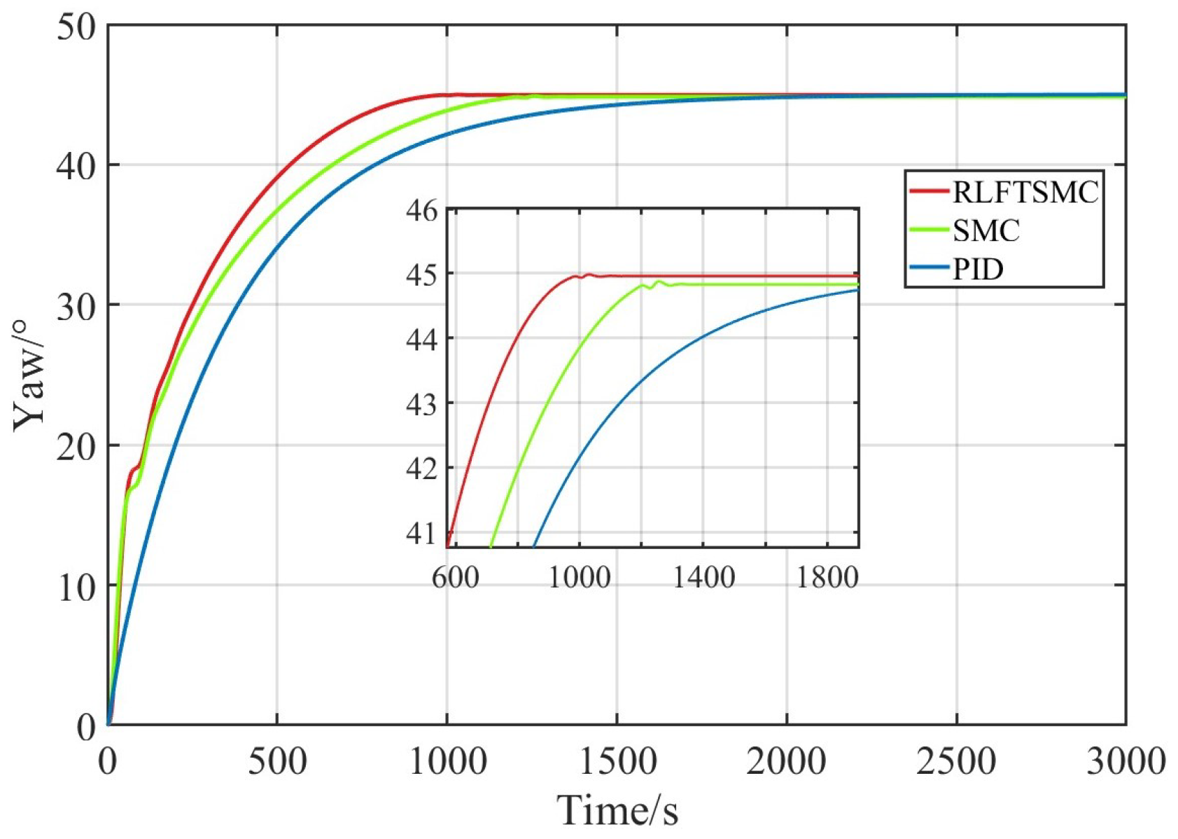
To verify the effectiveness of the proposed method, course control simulations were conducted and are explained in this section. At the beginning of the simulation, LDUUV is located at position $[x_0,y_0,z_0]=[0,0,0]$, with an initial attitude $[{\varphi }_0,{\theta }_0,{\psi }_0]=[0,0,0]$. The expected heading is set as ${\psi }_d={45}^{\circ }$. In the simulation, the forward speed remains at 4 knots. The specific simulation situation is shown in the following figures.

Figure 4 shows the convergence process of the reward function, which ultimately converges to a constant value.

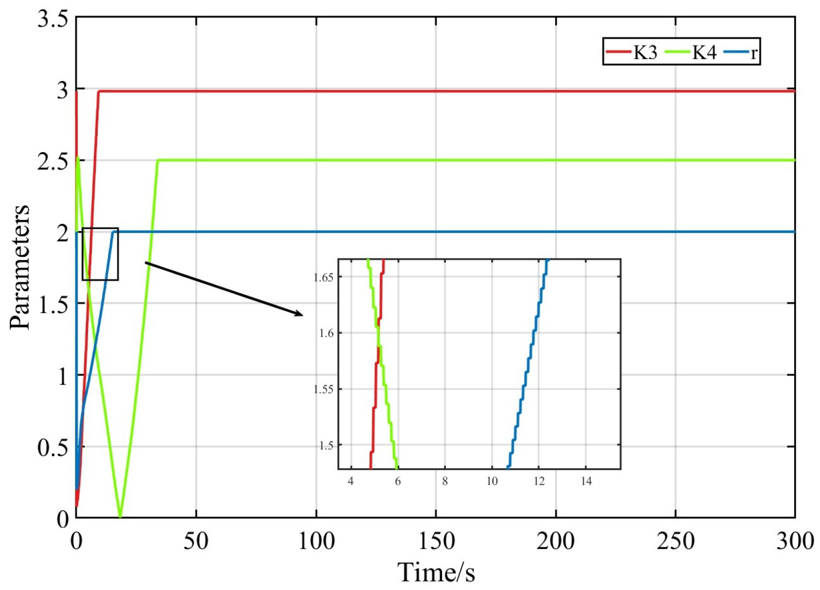
Figure 5 shows the parameter optimization process of sliding mode control based on reinforcement learning, starting from the initial initialization parameters and eventually converging to a fixed parameter. This also intuitively demonstrates the optimization process of reinforcement learning.

As shown in Figure 6, the control response of RLFTSMC is faster and more efficient than that of SMC and PID. When facing sudden or changing target states, RLFTSMC can achieve and stabilize the target value in a shorter period of time. In contrast, although SMC and PID can achieve the ultimate goal, it is significantly slower in response time and requires a longer time to converge to a steady state.

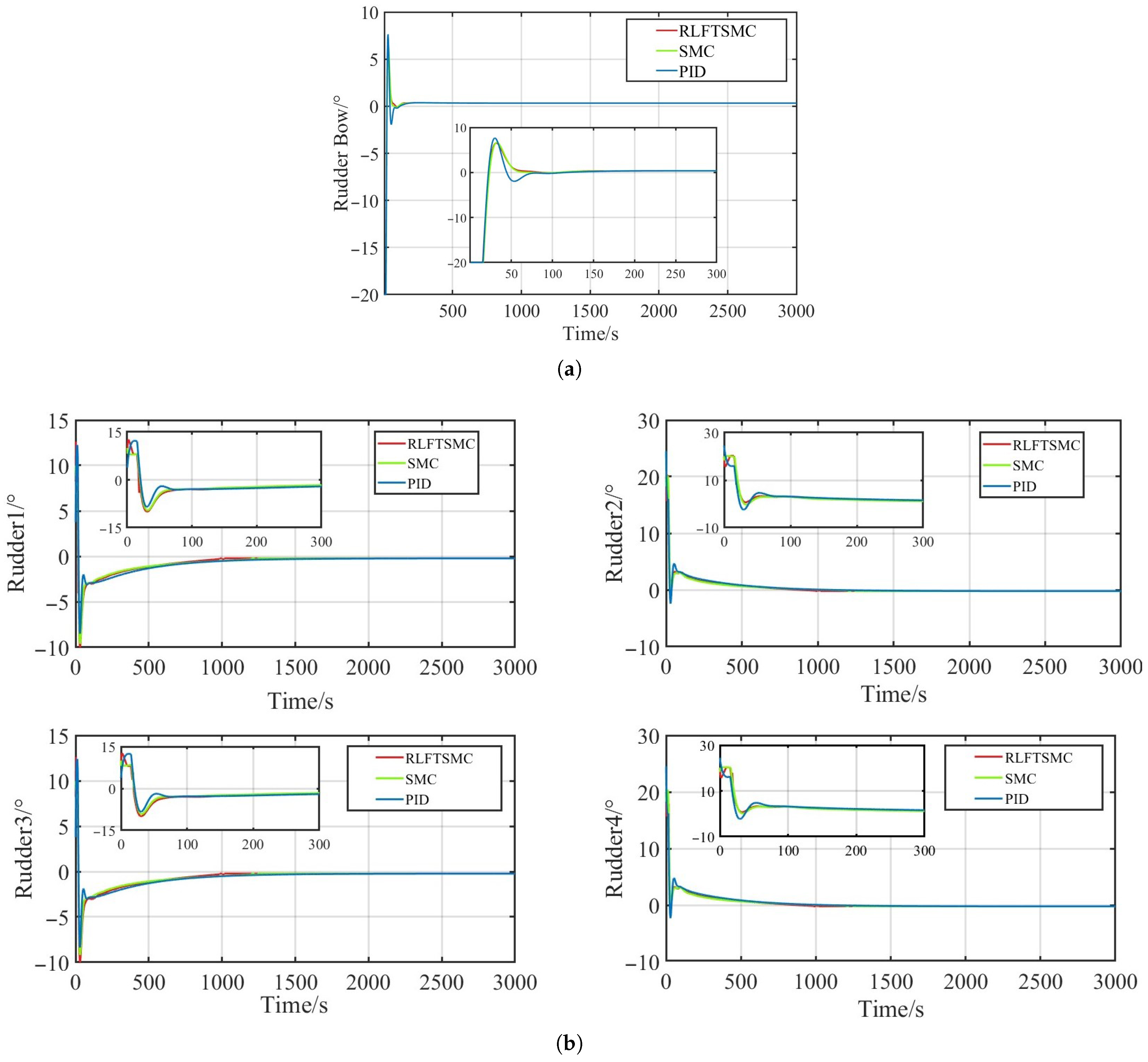
The simulation process is shown in Figure 7, where the control input of rudder 1 is equivalent to that of rudder 3, and the same relationship exists between rudder 2 and rudder 4. This symmetrical relationship between rudders indicates that the control strategy fully considers the coordination and balance of control inputs in system design, effectively avoiding uneven workload on the rudder surface, thereby improving the overall efficiency and stability of the system.

As can be seen from

Table 2. Quantitative comparison of tracking errors in course tracking.

Controllers	Heading Error (MAE/%)	Convergence Time (s)
PID	0.236	2190
SMC	0.378	1272
RLFTSMC	0.092	995

, the proposed RLFTSMC achieves the best overall performance in terms of transient response and control accuracy. Specifically, RLFTSMC reduces the convergence time by 21.7% compared to the SMC controller and by 54.6% compared to PID, demonstrating faster dynamic response under heading tracking tasks. In terms of tracking accuracy, the proposed RLFTSMC achieves the lowest mean absolute heading error, reducing the error by 60.8% compared to the PID controller and by 75.6% compared to the SMC controller. Although the SMC controller converges slightly faster than PID, it results in a significantly larger steady-state error, as shown in the heading response curves. These observations indicate that the PID controller achieves higher steady-state accuracy at the cost of slower convergence, whereas the SMC controller responds faster but suffers from higher residual error. In comparison, RLFTSMC effectively balances both convergence speed and steady-state precision, confirming its advantage in real-time heading control applications.

In addition, RLFTSMC demonstrated better smoothness and stability in the variation of rudder angle control input. Throughout the simulation process, the rudder angle variation pattern generated by RLFTSMC is more coherent, avoiding severe fluctuations or unnecessary high-frequency oscillations, thereby reducing wear on the actuator and system energy consumption. This enables RLFTSMC to effectively extend the system’s service life while ensuring fast convergence, improving the reliability and engineering applicability of the control system.

In contrast, although SMC and PID can achieve the goal, its steering effect response speed is slower, the convergence time is longer, and there may be significant fluctuations in the control input. This difference shows the comprehensive advantages of RLFTSMC in terms of control accuracy, response speed, and actuator protection, making it the preferred solution for achieving efficient and stable control scenarios.

4.2. Case 2: Path Following

Path tracking is an important task for verifying the stable navigation control performance of underwater vehicles. The goal of the task is to evaluate the ability of the LDUUV to accurately track along a set path in complex environments while examining the flexibility of attitude adjustment and the smoothness of control inputs during its navigation process.

In this case, we assume that the initial position of the underwater vehicle is $[x_0,y_0,z_0]=[0,0,0]$ and the initial attitude is $[{\varphi }_0,{\theta }_0,{\psi }_0]=[0,0,0]$, which means the underwater vehicle is in a stationary state on the horizontal plane, facing the reference path.

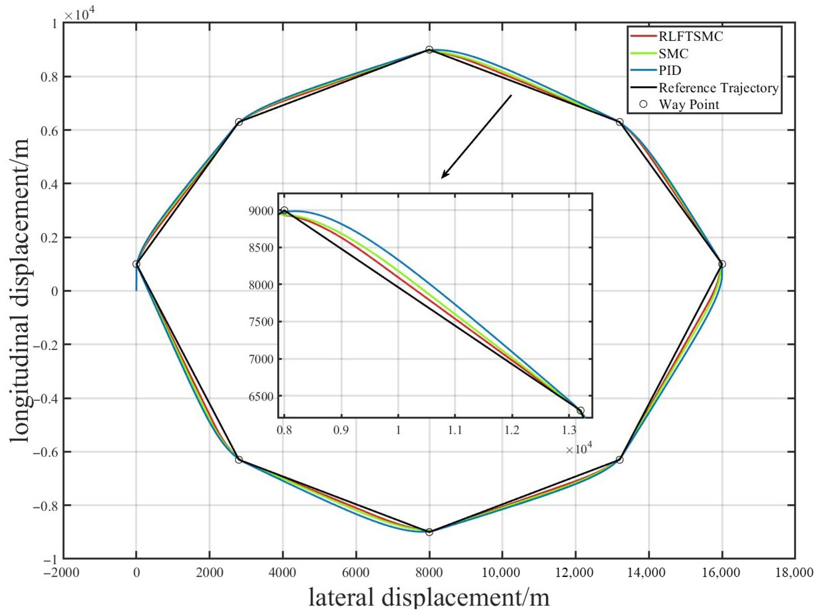
To verify the control performance of the underwater vehicle, a set of discrete waypoints was selected for path planning. This path covers various typical actions such as course tracking, depth control, and smooth cruising of the underwater vehicle, comprehensively examining the path-tracking ability and adaptability. These waypoints are set as wp1 = [0 1000 20], wp2 = [2800 6300 20], wp3 = [8000 9000 20], wp4 = [13,200 6300 20], wp5 = [16,000 1000 20], wp6 = [13,200 −6300 20], wp7 = [8000 −9000 20], wp8 = [2800 −6300 20].

The forward velocity was maintained at 4 knots throughout the entire simulation process. The expected trajectory and actual trajectory of the underwater vehicle are shown in Figure 8.

As shown in Figure 8, overall, the performance of RLFTSMC and SMC are almost the same, which is better than PID. Therefore, the robustness of RLFTSMC and SMC during heading was demonstrated. In addition, there is no serious chattering in the control inputs of both methods. It is evident from the figure that RLFTSMC has the best tracking performance. All three methods successfully complete the predefined path, including turning, straight-line cruising, and waypoint switching. However, RLFTSMC exhibits the highest accuracy in following the reference trajectory, particularly during turning transitions and long-distance curve segments.

Table 3. Quantitative comparison of tracking errors in path tracking.

Controllers	First Edge (m)	Second Edge (m)	Third Edge (m)	Fouth Edge (m)	Fifth Edge (m)	Sixth Edge (m)	Seventh Edge (m)	Eighth Edge (m)
PID	0.122	0.065	0.049	0.021	0.018	0.018	0.019	0.008
SMC	0.082	0.043	0.026	0.016	0.011	0.013	0.011	0.006
RLFTSMC	0.071	0.027	0.016	0.011	0.007	0.008	0.006	0.004

provides a segment-wise quantitative comparison. It can be observed that all three methods have sufficiently small errors in path tracking, but RLFTSMC performs more accurately because the relative error is the smallest among the three methods. RLFTSMC achieves the lowest tracking error on all eight path edges, with improvements of approximately 40–70% over PID, and 20–40% over SMC. This confirms that the proposed method offers higher precision in both linear and nonlinear maneuvering conditions.

Based on the above numerical results of two different scenarios and corresponding analysis, some discussions can be drawn as follows:

(1)

From a functional perspective, RLFTSMC, SMC, and PID are capable of performing various underwater vehicle maneuvers, including heading, depth, and waypoint tracking.

(2)

From the perspective of maneuverability and energy efficiency, the response speed of RLFTSMC is faster than SMC and PID. The disadvantage is that it requires more and faster rudder deflection, resulting in higher energy consumption.

(3)

From the perspective of parameter adaptability, RLFTSMC is a simpler tuning parameter compared to SMC and PID. As evident from the data analysis presented in Table 3, RLFTSMC yields the smallest tracking curve error compared to the other two methods.

5. Conclusions and Future Prospects

This article is dedicated to the issue of the LDUUV motion control with bow rudder and x-shaped stern rudders. A hybrid control framework is presented, which integrates model-based FTSMC with a reinforcement learning-based algorithm for real-time optimization of the controller. The proposed RLFTSMC utilizes the DDPG algorithm to dynamically adjust the controller gains, enabling adaptive performance in complex and uncertain underwater environments. The approach significantly mitigates chattering and enhances control smoothness, while preserving the finite-time convergence and robustness characteristics of FTSMC, as rigorously validated through Lyapunov stability analysis. To achieve coordinated control of the bow and stern rudders, an improved SQP control allocator is developed. This allocator solves a constrained nonlinear optimization problem that incorporates actuator limitations, energy efficiency, and control smoothness criteria. The numerical simulations validate the effectiveness of the proposed framework under model-unknown conditions. The RLFTSMC method outperforms conventional SMC and PID methods in terms of path tracking accuracy, convergence speed, and disturbance rejection capability. Future work will focus on extending the proposed framework to actuator failure scenarios. As actuator faults can significantly alter system dynamics and degrade control allocation performance, developing adaptive fault diagnosis and fault-tolerant strategies will be critical for enhancing the operational safety of underwater environments.