Quantitative Approach to the Preliminary Risk Analysis of Environmental Contamination Caused by Oil Spills from Offshore Oil and Gas Installations

Abstract

Despite improvements in oil spill prevention, recent data confirm that oil releases at sea are still a concern due to the severe environmental contamination potential. Regulations and standards addressing the safety of offshore oil and gas operations against major accident hazards require assessing and minimizing the risk to the environment caused by oil spills, as well as proving the effectiveness of emergency response plans. The present study proposes an innovative approach to the preliminary risk analysis of environmental contamination due to offshore oil spills, capable of orienting the engineering design of offshore installations and assessing the risk mitigation derived from the introduction of different safety barriers and emergency response strategies. New specific risk indexes and a novel procedure for their calculation were developed. The risk indexes are based on both the frequencies and the consequences of the spills, quantified as oil masses in each marine compartment. The approach allowed for obtaining robust risk indexes, also suitable for guiding the application of detailed oil spill risk assessment methods. A case study is presented to demonstrate the potential of the new approach.

1. Introduction

In the last two decades, the oil and gas industry has implemented extensive measures to prevent the occurrence of accidents resulting in oil spills [1,2,3]. However, the frequency of oil spill events from offshore installations does not evidence a definite decreasing tendency: actually, oil spill statistics (e.g., as those reported in [4,5,6,7]) present controversial trends depending on the sea area and the time period. For instance, about 1200 oil spills occurring worldwide between 1974 and 2010 were examined in [4], yet no definitive trend could be established. As a second example, data from Norway for the 2005–2024 period show a stabilization in the number of spills since 2013, followed by an increase in 2021–2022 compared with 2019–2020 and again by a decrease in 2023–2024 [7]. Accidents causing large uncontrolled releases of oil from offshore oil and gas facilities still occur, as confirmed by the Montara blowout (Timor Sea, 2009), the Deepwater Horizon accident (Gulf of Mexico, 2010), the Gannet Alpha leak (North Sea, 2011), and the Campos Basin spill (Brazil, 2011) [8,9]. Furthermore, the influence of climate change on offshore oil spill accidents has to be taken into account because of the possibility of an increase in oil spill risk [10].

A growing awareness of the risks involved in offshore oil and gas operations spread after the Deepwater Horizon accident, leading the European Union to a review of policies and regulations aimed at enhancing the safety standards of these activities. The process resulted in the release of Directive 2013/30/EU on the safety of offshore oil and gas operations [11], which establishes “minimum requirements for preventing major accidents in offshore oil and gas operations and limiting the consequences of such accidents”. The Directive focuses mainly on the protection of human lives and of the environment, not specifically addressing assets and reputation, that are in the responsibility of the operators. Thus, the report on major hazards required by the Directive aims at safeguarding the workers and the environment. In particular, when considering the potential impact on the marine environment, an Oil Spill Risk Assessment (OSRA) study has to be included in the report [12].

Despite the Directive poses a clear requirement concerning the need to assess the risk to both people and the environment, no specific guidelines are available to support its application. In particular, the Directive explicitly defines risk as the combination of the frequency of an accidental event and the severity of its consequences, in accordance with the definition introduced by the ISO guidelines on risk management [13,14] and with the definition of risk applied in the context of the control of major accident hazards in the chemical and process industry [15,16]. However, conventional quantitative risk assessment models usually address—for both onshore and offshore activities—only the risk of human fatalities, usually expressed as local specific individual risk or societal risk [17]. Despite the large number of OSRA methods published in the technical literature, no widely accepted approach is available for the quantitative assessment of the risk of environmental contamination caused by oil spills. Moreover, no agreement is present on the risk indexes expressing the risk to the environment. Thus, a standardized methodological approach for the quantitative assessment of the risk to the environment of major accidents involving oil spills is still lacking [18,19,20].

In the present study, an original metrics for a preliminary risk analysis of the environmental contamination caused by offshore oil spills in the context of major accident hazards and a set of novel risk indexes were developed. The novel risk indexes developed are based both on the likelihood of oil spills and on their consequences. The consequences of oil spills are expressed in terms of the amounts of oil present in each sea compartment, i.e., as the masses of oil floating on the sea surface, submerged in the water column, sedimented on the sea floor, and beached along the coastline. A procedure supporting their calculation is also provided, suitable for the use in the framework of an initial Oil Spill Risk Assessment of offshore oil and gas installations. The screening method developed, which takes into account both topside and subsea releases, allows considering the influence on risk of different safety measures and of different contingency response actions, in order to quantify the risk reduction due to emergency response, in compliance with the requirements of Directive 2013/30/EU. Furthermore, it supports the engineering design of oil and gas facilities, because the new indexes make it possible to include the risk to the environment in the decision process about the preferred design option.

This paper has the following structure: the state of the art of OSRA procedures is presented in Section 2, in order to highlight the need for a novel OSRA method specifically addressing the environmental contamination caused by oil spills. In Section 3, the new risk indexes for expressing the risk of environmental contamination are introduced and the methodology for their calculation is described. In Section 4, a case study is presented. Section 5 and Section 6 report, respectively, the results of the case study and the discussion of the main findings, while some conclusive remarks are drawn in Section 7.

2. State-of-the-Art of OSRA Methods

A wide number of risk assessment methods addressing the management and control of the environmental risk of oil spill accidents in offshore oil and gas installations have been proposed in the literature. Most of the methods were developed after the Deepwater Horizon blowout that can be considered a cornerstone event when considering the environmental consequences of oil spills at sea. An overview of a few of these methods is provided by the study of Neves et al. [21], also reporting a comparative analysis of their features and outputs.

As documented in [22,23], OSRA procedures can take significant advantage of the recent progress in the comprehensive simulation of oil releases provided by oil spill consequence models (as those proposed e.g., in [24,25,26,27,28,29,30,31,32,33,34,35,36,37]). More specifically, the increase in the computational resources available allows applying routinely the “stochastic” evaluation of the consequences of oil leakages. In fact, the simulation of an oil release can be carried out assuming different starting dates, so to reflect the variety of meteorological and oceanographic situations (usually defined “metocean” conditions), which could be present when the spill occurs, leading to different fates and transport patterns of the oil [38]. The results of the stochastic consequence analysis are often reported by means of maps showing, for a spill occurring in a given location, the spatial distribution of the percentage probability of the oil presence. Examples of maps with the oil presence probability can be found, for instance, in [39,40]. While these maps are effective tools for the description of the results of the probabilistic assessment of the consequences of a given spill event, they do not account for the occurrence frequency of the accident. Hence, these maps “per se” are not suitable to express the risk to the environment in accordance with the definition of risk introduced by the Directive 2013/30/EU.

Therefore, the focus of the present state-of-the-art section was limited to methods in which the risk of accidental spills is assessed as a combination of the yearly frequency of occurrence of the spills and of their consequences, since only this category of methods delivers risk indexes complying with the requirements of Directive 2013/30/EU. Nevertheless, in order to obtain a more complete picture of the available methodologies, the methodologies developed for oil spills from tankers and, more generally, from ships, were also considered, since most of them can be adapted to oil and gas facilities with minor modifications.

The OSRA approaches taking into account both the frequencies and the consequences of spills can be classified in three categories, having an increasing complexity [41]: (1) source-based methods; (2) exposure-based methods; and (3) damage-based methods. While in source-based procedures the consequences of the oil spills are expressed by the amount of oil spilled, in exposure-based procedures, they correspond to the exposure, i.e., to the impact of the oil on the ecological resources in the oiled area. In damage-based methods a further step is added to the analysis of the consequences of the oil spills, obtaining the recovery times of the species impacted by the oil. A more detailed explanation of the features of these three categories of OSRA methods is reported in the Supplementary Material.

Even acknowledging the recent advances in OSRA methods, which mostly implement exposure- or damage-based approaches, the existing procedures still present some weaknesses, mostly deriving from five different factors.

Firstly, most procedures (e.g., those described in [42,43,44]) focus only on the sea surface and/or the coastline, neglecting the other marine compartments. Even those considering the dissolution and dispersion of oil in the water column do not take into account the sea bottom [45,46,47]. However, the Deepwater Horizon blowout proved that, despite the sunken oil is not directly visible, its amount may be a relevant percentage of the spill volume, so that the sea bottom can be heavily affected by the consequences of an oil spill [48].

Secondly, the existing approaches (e.g., those proposed in [45,46,47,49]) are qualitative or semi-quantitative. Some of them make use of discrete correlations for the estimation of the consequences of the oil spills, which are not always able to discriminate the effects of different releases, in particular when involving small volumes of oil [50]. In this regard, it should be remarked that in Europe operators of offshore oil and gas installations are required to conduct risk analyses considering as targets both people and the marine environment [11]. This requirement is coherent with the fact that, since more than 25 years, the European legislation includes the environment beside the human health, when considering the targets of major industrial accidents [51]. Rather intuitively, in spite of the different goals of these studies, they should be carried out consistently and with the same level of detail. However, this has not been the case up to now, due to the lack of quantitative methodologies for analyzing the risk of environmental contamination caused by major accidents.

A third limit of the existing semi-quantitative OSRA methods is related to the unavailability of the input data necessary for the evaluation of the exposure. For instance, the ERA Acute methodology needs to input the spatial distribution of the valuable plants and animals in a 10 km × 10 km grid, and monthly averaged data for expressing the temporal distribution of the species. However, such detailed information is currently available only for a minority of sea areas worldwide, as confirmed by [52]. Consequently, very often, only a qualitative estimate of the impact of a spill on the biological resources present in the oiled zone can be carried out, as required, e.g., in the procedure described in [46].

The fourth issue of the existing semi-quantitative procedures is related to the computational time. In fact, since running a biological model with a fine spatial and temporal resolution in order to estimate the exposure requires a significant effort, usually only worst case meteorological and oceanographic conditions are taken into account when simulating the fate and the trajectory of the oil [52]. However, these metocean conditions could be extremely rare, and their application may not provide a representative figure of the effects of the oil spill, in terms of both the more probable position of the oiled area and of the extension of the ecological impact. Furthermore, basing the emergency response on worst case simulations, without considering less severe but more frequent metocean situations, could lead to an improper planning of the response, for instance in terms of the optimal positioning of the contingency equipment.

A further limit of the procedures available to date is the high degree of uncertainty affecting the environmental risk results. This uncertainty derives from the uncertainty in the consequences of the oil spills, expressed as impacts on the ecological components or recovery times of the impacted population. In fact, moving along the consequence chain of an oil spill scenario, i.e., passing from the amount of the spill to the simulation of the fate of the oil, and from the latter to the evaluation of the impact on the ecological species and, in case of damage-based approaches, to the estimation of the restitution times, an increasing number of assumptions and input parameters are incorporated into the risk metrics, leading to the propagation and amplification of uncertainty, as exemplified in [53,54,55]. In particular, the calculation of the impact and of the damage of the natural resources, which is based on a biological model requiring as an input the spatial and temporal distribution of the vulnerable ecological components, usually provides a significant contribution to uncertainty. In fact, a huge uncertainty in the risk results hinders the possibility of including them in the engineering decision making processes on the design of the oil and gas facilities, as well as of efficiently comparing their values with risk acceptability criteria [53]. Therefore, in order to reduce the uncertainty of the consequences of the oil spills, it may be considered to limit the consequence analysis at an earlier stage, immediately after the simulation of the fate of the spilled oil and before the application of a biological model. In fact, the results provided by oil spill fate models are represented by the so called “oil budget”, that is by the temporal trend of the amounts of oil in the different marine compartments.

It has also to be remarked that the final aim of risk assessment is the reduction in risk, which is a progressive process supporting the objective of continuous improvement. This can greatly benefit from the comparison of risk figures with risk acceptability criteria established by public authorities, which should stimulate the identification and implementation of additional technical, operational, and organizational safety barriers [13,41,56]. Therefore, the implementation of a risk metric coherent with current acceptability criteria would be an important advantage also in methods addressing the preliminary risk screening.

Thus, the review of OSRA methods available in the literature to date clearly shows the need to improve the existing approaches for the assessment of the environmental risk deriving from oil spills and the metrics implemented to express the risk of environmental contamination [53].

3. Methodology

The purpose of the innovative methodology developed in the present study for preliminary risk analysis of environmental contamination caused by oil spills from offshore oil and gas installations is twofold. On the one hand, the risk results may be used to guide the design of oil and gas facilities, making it possible to compare the risk to the environment of oil spills deriving from alternative design options, as well as the evaluation of the effectiveness of alternative safety barriers in reducing the risk values. On the other hand, since the novel method can include the contribution of emergency response actions, it can be applied for quantifying the influence of these actions on the final risk figures.

Moreover, in order to overcome the weaknesses of the methods adopted to date, the original method developed within the present study: (1) provides consistent risk indexes addressing all marine compartments; (2) is fully quantitative; (3) is applicable worldwide (even there where accurate mapping of the vulnerable resources is not yet available); (4) considers a broad spectrum of meteorological and oceanographic conditions; and (5) provides a preliminary estimate of the risk of environmental contamination based on robust risk indexes, which are not affected by the uncertainties introduced by biological models and which can be used in the successive application of exposure- and damage-based methods.

3.1. Definition of Specific Risk Indexes for the Contamination of the Marine Environment

As a starting point, a specific risk metric is defined for the four marine compartment that may be contaminated by the oil spill: the sea surface, the water column, the coastline, and the sea bottom. The risk metric introduced is based on the amount of oil impacting each compartment and on the frequency of such an occurrence. In particular, four cumulative F(m_c) risk curves are defined, one for each compartment, expressing the yearly cumulated occurrence frequency F of an oil spill resulting in a mass of oil equal to or higher than m_c in the compartment c considered:

• F(m_seasur) expressing the yearly cumulated occurrence frequency F of an oil spill resulting in a mass of oil floating on the sea surface equal to or higher than m_seasur;
• F(m_watcol) expressing the yearly cumulated occurrence frequency F of an oil spill resulting in a mass of oil submerged in the water column equal to or higher than m_watcol;
• F(m_coastl) expressing the yearly cumulated occurrence frequency F of an oil spill resulting in a mass of oil beached along the coastline equal to or higher than m_coastl;
• F(m_seaflo) expressing the yearly cumulated occurrence frequency F of an oil spill resulting in a mass of oil deposited on the seafloor equal to or higher than m_seaflo.

The mass values m_seasur, m_watcol, m_coastl, and m_seaflo, which represent the terms of the so called “oil budget”, i.e., the mass balance of the oil spill, are typically provided as an output by oil fate and trajectory models [57]. As better explained in Section 3.2, the mass values depend on the features of the spill, on the physical and chemical properties of the oil, on the morpho-bathymetry of the area where the oil is dispersing, on the environmental conditions in this area during and after the release, and on the emergency response strategies adopted for contrasting the spill. All these data represent the input to the oil fate and trajectory model to be run in the application of the methodology. Instead, they do not depend on the fauna and flora potentially affected by the oil (as, e.g., coral reefs, mangroves, seagrass, etc.). Actually, the amounts of oil in the four sea compartments, which represent the consequences of oil spills in the risk indexes introduced in the present study, are key factors in causing the negative effects inflicted by the spill to the marine compartments, thus being important terms for expressing the risk to the environment [58]. In fact, these data are among the information gathered in the post-accident analysis of spill events (as reported, for instance, in [59]).

The F(m_c) risk curves may be calculated for a single spill i (for instance the release caused by the rupture of the riser of an offshore facility), considering all the metocean conditions which could be present when the spill occurs, following the procedure described in Section 3.2. However, it is also possible to calculate the curves for a set of oil spills N_ss, that is, spills with different release rate and duration, as, for instance, all the topside releases or all the subsea spills considered possible for a facility of interest, or even the whole set of the topside and subsea spills N_spill which can occur on an installation.

From each F(m_c) risk curve, a point-value risk index EXm_c, corresponding to the amount of oil yearly expected in the sea compartment c, may be obtained by means of Equation (1):

$${EXm}_c={\int }_0^{\mathrm{\infty }}F\left(m_c\right)·d{m}_c$$

(1)

Thus, from the four F(m_c) risk curves previously defined, the following point-value risk indexes are derived:

• EXm_seasur, expressing the mass of oil yearly expected to float on the sea surface;
• EXm_watcol, expressing the mass of oil yearly expected to be submerged in the water column;
• EXm_coastl, expressing the mass of oil yearly expected to beach along the coastline;
• EXm_seaflo, expressing the mass of oil yearly expected to sediment on the sea bottom.

The calculation process of Equation (1) is introduced in Section 3. Indeed, each point-value risk index coincides with the area beneath the correspondent F(m_c) curve, which takes into account all oil spills (from the smallest to the largest) in all possible metocean conditions. In this way, it allows overcoming the fourth limit of the existing methods mentioned in Section 2. It is important to notice that the cumulative risk curves used to derive the risk indexes are similar to the F_fat(N_fat) risk curves expressing the cumulative frequency, F_fat, of an event causing a number of fatalities at least equal to N_fat, which represent the most common approach for expressing societal risk in the context of the risk analysis of major accident hazards [16]. Moreover, the point value risk indexes which can be obtained from each F(m_c) curve are analogous to the potential life loss index derived for a F_fat(N_fat) curve, representing the yearly expected number of fatalities and coinciding with the area beneath the F_fat(N_fat) curve [60]. Thus, the indexes proposed for the quantification of the environmental risk are built on a well-known and broadly recognized risk metric, extending to the environment an approach widely adopted when calculating risk to people. A similar method has proven to be effective also in the quantification of the environmental damage of major accidents resulting in oil spills from onshore pipelines [19,61].

In the definition of the new risk metrics, the simplifying assumption of considering four separate sea compartments was made. Actually, while this schematization is functional to the calculation of risk, from an ecological point of view, the marine compartments are strictly interconnected. However, as reported before, a strong point of the new OSRA approach is the calculation of the environmental risk for all the marine compartments.

3.2. Calculation of the Risk Indexes

In order to obtain valuable results, consistency should be assured among the new risk indexes calculated for the environment and the conventional risk indexes calculated for humans. 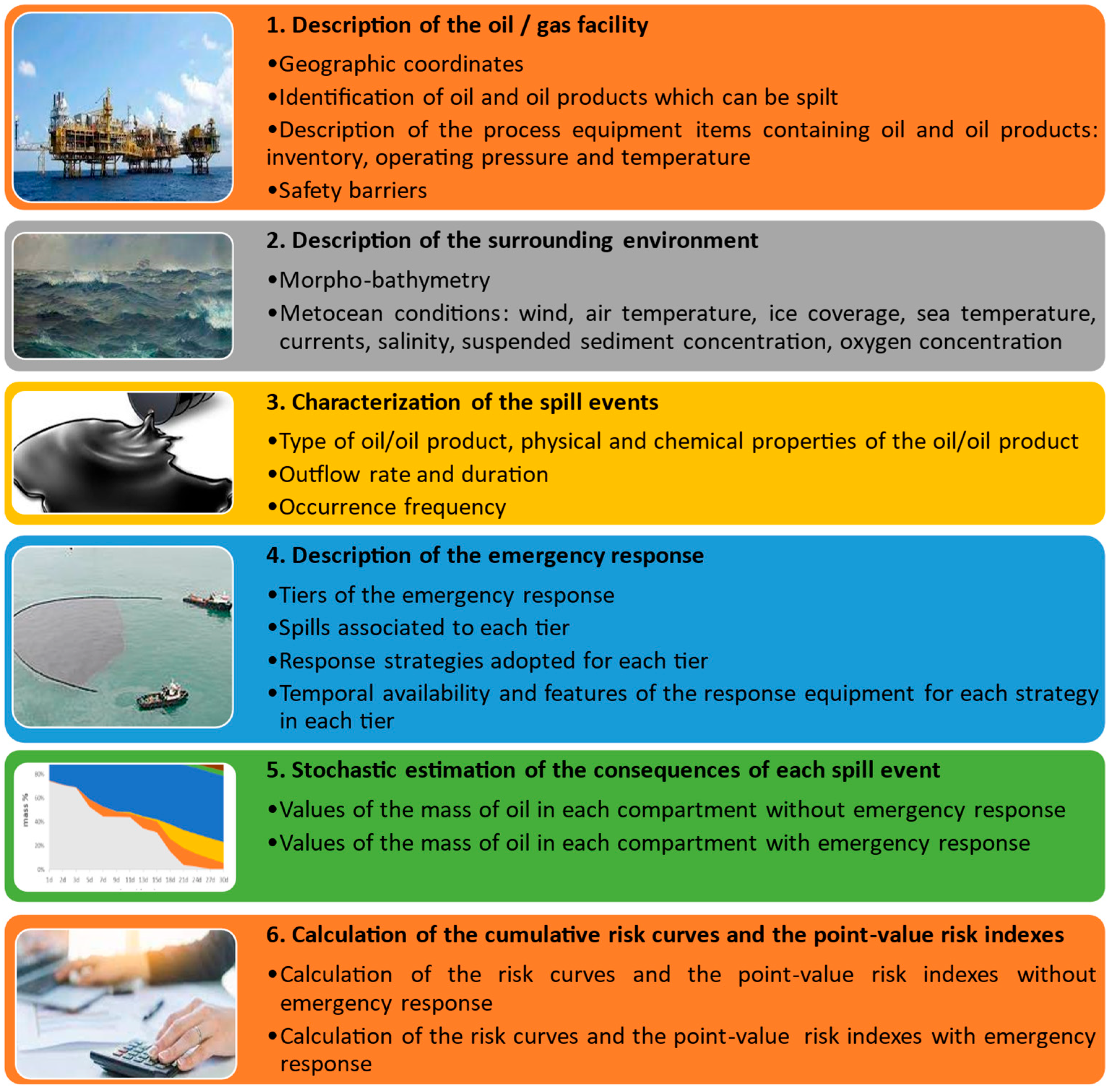Therefore, the risk screening approach proposed herein for the calculation of the environmental risk indexes is based on the extension of that used in conventional quantitative risk assessment in order to calculate the risk to people caused by major accidents (as fires, explosions, and toxic releases) [15,16,62]. The methodology developed for the calculation of the risk indexes consists in six steps, as shown in Figure 1.

With reference to Figure 1, the six steps correspond to the gathering of the different data required by the new risk approach (step 1, step 2, and step 4), the application of a hazard identification technique and of suitable source models (step 3), and the application of an oil fate and trajectory model (step 5), finally leading to the last stage, i.e., the calculation of the new risk indexes (step 6).

In more detail, the first step of the procedure consists in gathering the information about the risk source. This requires to determine the latitude and longitude of the facility, since they are typically assumed as the coordinates of the spill origin. Furthermore, it is necessary to identify the process units in which oil and oil products are present and to collect the values of their inventories, as well as their pressure and temperature operating conditions. Even the presence of safety barriers has to be considered, such as, for instance, alarms, safety interlocks, isolating valves, and catch basins.

In step 2, the meteorological and oceanographic data in the area that may be impacted by the oil have to be retrieved. The spatial and temporal resolution of the data must be consistent with the requirements of the software used to simulate the trajectory and fate of oil spills, as described in step 5. In addition, since each spill has to be simulated using different starting dates to account for seasonal and interannual variability in metocean conditions, the data should cover a period of several years. While ten or more years are very often recommended [63], shorter time spans (down to a single year) may be acceptable for screening studies in the context of preliminary risk analyses [46,64]. Hindcasts of metocean data (e.g., wind, air temperature, ice coverage, currents, seawater temperature, salinity, oxygen concentration, suspended solid concentration) are currently available for all the seas of the world (even for the Arctic or for developing countries), making straightforward the application of the procedure to any sea area. In future, the ongoing improvement in the quality of these data will positively affect the method, providing more precise risk values. In order to capture the temporal variability of these data and, consequently, to obtain a realistic representation of all the possible trajectories of the oil, metocean conditions usually refer to a multi-year period [38]. More and more sources make these data available worldwide. For instance, the European Union’s Earth Observation Programme has developed the Copernicus Marine Environment Monitoring Service, which provides full, free, and open access to ocean data on a global scale (i.e., for all seas of the world) [65]. Similarly, the HYCOM consortium sponsored by the US National Ocean Partnership Program makes available metocean data on a global scale [66]. Clearly enough, uncertainties may be present in such data and should be carefully considered according to their specific source (e.g., as reported in [4]). However, a discussion of this aspect is out of scope of the present study.

Step 3 requires the quantitative characterization of all the oil spill events to be considered for the calculation of the risk indexes. In the case of offshore oil and gas installations, a structured approach called ENvironmental hazards IDentification (ENVID) can be applied for the identification of the potential events leading to oil spills. This technique consists of workshops involving experts in safety and in other engineering disciplines (e.g., maintenance and operations) [46]. However, the standard hazard identification methods typically applied in the context of the risk of major accidents [67] and, more specifically, those proposed for offshore installations [41,68] can be used too. In fact, the selection of the hazard identification technique falls upon the risk analyst. After identifying the oil spills, each oil has to be characterized with its physical and chemical properties. In fact, as a function of the inventories and operating conditions of the equipment items from which the oil spills might originate (retrieved in step 1) and of the oil properties (retrieved in step 2), the rate and the duration of each spill are calculated, using appropriate source models (e.g., as those described in [62,69,70]). Furthermore, an annual occurrence frequency f_spill,i is assigned to each spill i. It has to be recalled that the presence of safety barriers strongly influences the results of step 3. In fact, preventive safety measures reduce the spill frequencies, while protective safety measures can diminish the outflow rate and the duration of the loss of containment events.

With respect to step 4, usually in the case of offshore installations a tiered preparedness and response approach is recommended as the underlying basis for the preparation of the oil spill contingency plan. This approach assigns oil spill events having different severity to tiers characterized by different response capabilities, using the amount of oil spilled as an estimate of the severity of the spill. In fact, the emergency plan has to address the spills identified in the risk assessment for each response level [71,72].

In order to estimate the consequences of each spill (step 5), the application of an oil fate and transport model to the oil spills identified in step 3 is needed. The fate and transport of the oil depend on the morpho-bathymetry and on the metocean data retrieved in step 2, and, in case emergency response is considered, on the response strategies described in step 4. As explained in step 2, each spill has to be simulated in different metocean conditions, running stochastic simulations. While the number of stochastic simulations needed for robust results depends on the specific case study, generally a minimum of 50 simulations seems to be required [55]. A review of oil spill models is reported in [57]. Even if the novel risk assessment methodology has a general validity and is not based on the results of a specific software tool, the application of a model able to take into account emergency response is necessary to carry out the required calculations. The choice of the model to adopt is let to the risk analyst. The analysis of the fate of the spilled oil should be carried out twice: in the first run, no emergency response is considered; in the second run, the oil amounts in each compartment are determined considering emergency interventions intended to mitigate the effects of the spilled oil. Rather intuitively, these amounts are influenced by emergency response actions, as shown further on in Section 5 and Section 6.

Clearly, the amount of oil present in each environmental compartment changes as a function of time. The oil on the sea surface is maximum at the end of the release, then it decreases mainly due to the evaporation of the light fractions, to the entrainment of oil in the water column and to the stranding of the oil, when the slick nears the coastline. A similar trend, typically slightly delayed with respect to the one of the floating oil, is observed also for the oil in the water column. In fact, the oil enters the water column from the slick and progressively exits from this compartment because of its deposition on the sea bottom. However, the sedimentation of the oil on the seabed and its deposition on the shoreline usually begin with some delay with respect to the start of the spill, when the oil slick and the underlying water column with the submerged oil approach the coastline and the shallow water in front of it. It might also be that the oil never reaches the coast, if the combined action of the winds and of the currents drifts the slick toward the open sea. In this case, the oil on the sea surface disappears after a certain time, without any beaching, and the oil in the water column sinks and settles down onto the seafloor. In the end, on a different and significantly longer time scale, the oil deposited on the beach and on the seafloor gradually decreases due to the biodegradation processes. Further details about the oil weathering and transport processes and their evolution over time are reported elsewhere [73,74].

From the above discussion, it is evident that a reference time has to be defined for the estimation of the amounts of oil in each compartment, m_c, necessary for the calculation of the risk indexes. In order to highlight the influence of the emergency response, selecting a time related to the end of the emergency actions, when the contribution of these actions to the reduction in the oil amount in each sea compartment is maximum, is suggested. Values of this time are typically reported in oil spill emergency response plans, depending on the response tier [46]. Indeed, it has to be noted that contamination may continue after the end of the emergency response. In fact, the amounts of oil in each compartment evolve over time, and the timing of maximum contamination differs among compartments for a given simulation (i.e., a specific combination of spill and starting date). Furthermore, for a given compartment, the temporal evolution of the oil mass differs from one simulation to another. However, without fixing a reference time, it would not be possible to compare the oil mass values caused by a given spill in a given compartment on different starting dates. Thus, in the present approach, the time at which the emergency response ends is taken as a reference time for the comparison purposes, and should not be considered as the time at which oil diffusion is ended.

Oil fate and transport models are generally implemented in software codes, which provide as an output the values of m_c,i,j, i.e., the mass of oil present at the selected reference time in the sea compartment c as a consequence of spill i occurring on date j, to which specific metocean conditions are associated. These oil masses m_c,i,j are calculated in step 5 of the procedure for all the spill events considered, N_spill, for all the dates on which the spills are assumed to start, N_sim, and for all the four marine compartments c (with c = seasur for the sea surface, c = watcol for the water column, c = coastl for the coastline, and c = seaflo for the seafloor).

In order to calculate the final risk indexes (step 6), the frequencies and the consequences of the spill events have to be combined. Since all the N_sim starting dates of a spill, i.e., all the sets of the corresponding metocean conditions, have the same occurrence probability, P_met, this probability can be determined as follows:

$$P_{met}=1/N_{sim}$$

(2)

Consequently, the frequency of spill i occurring on a date j, i.e., in the presence of a set of metocean conditions, f_met,i is given by

$$f_{met,i}=f_{spill,i}{·P}_{met}$$

(3)

Thus, a total of N_sim couples (m_c,i,j, f_met,i) can be obtained for each compartment c and spill i. The cumulated frequency values F_c,i, can be derived as a function of the frequency values f_met,i, so that N_sim couples (m_c,i,j, F_c,i) are calculated, representing the points of the F(m_c) curve for spill i and compartment c. Furthermore, the point value risk index expressing the mass of oil yearly expected in compartment c in case of spill i can be determined as follows:

$${EXm}_c=\sum _{j=1}^{N_{sim}}{f}_{met,i}·m_{c,i,j}$$

(4)

In fact, based on the correlation among the cumulated frequency values F_c,i, and the frequency values f_met,i, the following equivalence can be easily demonstrated:

$$\sum _{j=1}^{N_{sim}}{f}_{met,i}·m_{c,i,j}=\sum _{j=1}^{N_{sim}}{F}_{c,i}·{\mathsf{\Delta }m}_{c,i,j}\approx \underset{0}{\overset{\infty }{\int }}F\left(m_c\right)·d{m}_c$$

(5)

Similarly, when considering a number of spills N_ss, with 1 < N_ss ≤ N_spill, a total of N_ss·N_sim couples (m_c,i,j, f_met,i) can be derived, from which N_ss·N_sim couples (m_c,i,j, F_c,i) are obtained. The latter represent the points of the F(m_c) curve for compartment c caused by the N_ss spills. Correspondingly, the point value risk indexes expressing the mass of oil yearly expected in each compartment c when considering the N_ss spills, are determined as follows:

$${EXm}_c=\sum _{i=1}^{N_{ss}}\sum _{j=1}^{N_{sim}}{f}_{met,i}·m_{c,i,j}$$

(6)

4. Application to a Case Study: Data and Assumptions

The developed methodology was applied to an oil facility, both to illustrate the step-by-step application of the procedure and to test its capabilities. The selected installation corresponds to a Floating, Production, Storage, and Offloading (FPSO) unit with subsea wells and export through offloading. In fact, this kind of offshore unit represents a relevant case study, because it can give rise to both topside and subsea oil spills, having highly different spill amounts and durations and requiring different emergency response interventions. 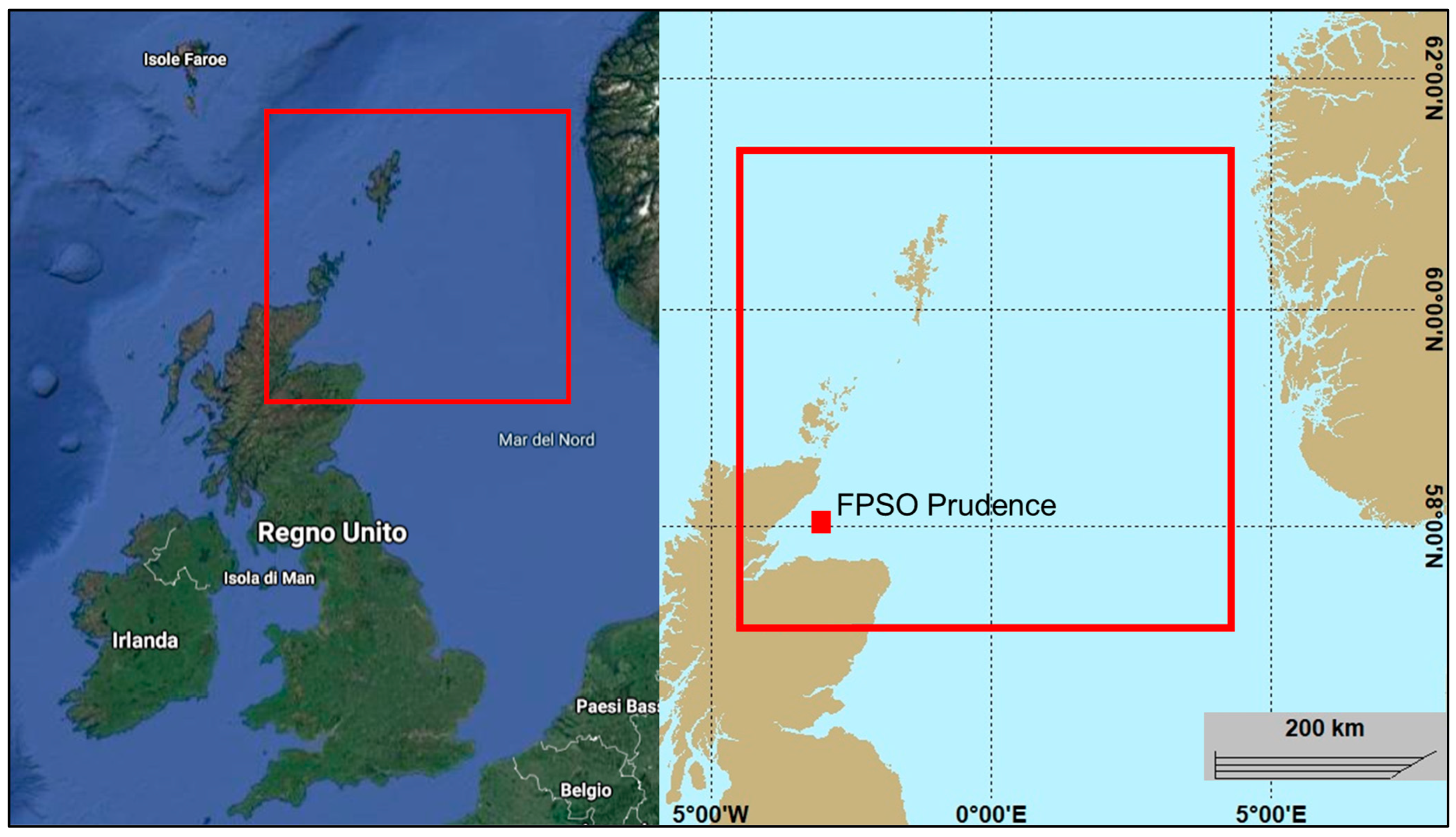The facility selected is that considered by the following [46]: a fictitious FPSO unit named Prudence, in the production phase, sited in the North Sea off Scotland (UK), as shown in Figure 2.

The oil produced at the Prudence field is similar to the Statfjord C blend, a light low-sulphur oil produced in an oil field sited northern to the FPSO [75,76]. A diesel tank is also present on the Prudence FPSO [46].

The Prudence facility is equipped with all the safety measures required by the current regulations in the region considered and by the sectorial good practices, as blowout preventers, subsea capping and containment systems, subsea leak detection systems, integrity monitoring of all the tanks and process equipment units, monitoring by personnel of all the crude oil unloading and the diesel uploading operations. Further details on the safety systems are reported in [46].

The average water depth at the Prudence field is equal to 49 m, while the minimum distance between the FPSO and the coast is 24 km. Suitable data about the winds and the currents were obtained from the Copernicus Marine Environment Monitoring Service [65,77], which provides 2D 6-h-averaged wind data with a spatial resolution (expressed as latitude × longitude) of 1/4° × 1/4° (approximately 27.8 km × 14.7 km) and 3D 24-h-averaged current data with a horizontal spatial resolution of 1/12° × 1/12° (approximately 9.3 km × 4.9 km) and considering up to 50 vertical levels. Data referring to a period of five years (2013–2017) were considered for the simulations of the oil spills. The air and sea temperatures were both assumed equal to 8 °C [78]. For salinity, the value of 34.5 ppt was adopted [79]. The dissolved oxygen concentration was taken equal to 10 mg/L [80], while for the suspended particulate matter the value of 0.8 mg/L was used [81]. For the sake of simplicity, the temperatures, the salinity, the oxygen, and the suspended solid concentrations were considered constant in time and spatially uniform.

The potential oil spills assigned to the Prudence facility were identified by a dedicated ENVID study reported in [46], based on the features of the installation and on the available safety barriers.

Table 1. Oil spills identified in the ENVID study carried out for the Prudence FPSO (adapted from [46]).

Spill ID	Spill Category		Oil Type	Rate	Duration	Total Mass	Temperature	Frequency fspill,i	Response Tier
/	/		/	t/d	h or d	t	°C	ev/y	/
S1	blowouts from production wells		crude blend	2227	2 d	4454	65	6.73 × 10−5	3
S2					5 d	11,135	65	2.60 × 10−5	3
S3					15 d	33,405	65	2.91 × 10−5	3
S4					50 d	111,350	65	3.06 × 10−5	3
S5				1513	2 d	3026	65	9.68 × 10−5	3
S6					5 d	7565	65	3.74 × 10−5	3
S7					15 d	22,695	65	4.18 × 10−5	3
S8					50 d	75,650	65	4.40 × 10−5	3
S9	leaks from subsea systems and risers	small flowline leak	crude blend	345	2 h	28.7	20	2.59 × 10−3	1
S10		large flowline leak		1242	12 h	621	20	9.10 × 10−4	2
S11		small riser leak		384	1 h	16	20	9.36 × 10−4	1
S12		large riser leak		2904	1 h	121	20	2.66 × 10−3	1
T1	leaks from the process system	large leak second stage separator	crude blend	2064	0.5 h	43	40	9.69 × 10−4	1
T2		small leak second stage separator		252	2 h	21	40	7.10 × 10−3	1
T3	leaks from the FPSO	offloading buoy	crude blend	103,632	1 h	4318	8	9.00 × 10−5	3
T4		fire and explosion in cargo tank or engine room, structural failure, ship collision	crude blend	132,444	2 h	11,037	8	2.10 × 10−4	3
T5		loss of position	crude blend	300	24 h	300	8	7.30 × 10−4	2
T6		leak from tank	diesel	646	48 h	1292	8	4.68 × 10−4	2

provides an overview of these events.

A total of 12 subsea spills (S1 ÷ S12) and 6 topside spills (T1 ÷ T6) were identified for the facility. Subsea leakage events correspond to blowouts or to leaks from subsea systems and risers, while topside spills correspond to releases from either the process system or the FPSO. Thus, the total number of spills of the installation N_spill is equal to 18 loss of containment events, belonging to four spill categories. Since all the spills origin in a rather small area, for the sake of simplicity they can be assumed as having the same geographical coordinates. Only spill T6 involves diesel fuel, while in all the other events crude oil is released. The leakage events are characterized by rather different outflow rates (from 25 t/d to 132,444 t/d), durations (from 0.5 h to 50 d), total released mass values (from 16 t to 11,350 t), spill temperatures (from 8 °C to 65 °C), and occurrence frequencies (from 2.60 × 10⁻⁵ ev/y to 7.10 × 10⁻³ ev/y). Furthermore, as shown in the last column of Table 1, each spill is assigned to a different emergency response level.

In fact, the oil spill emergency response plan of the Prudence FPSO is organized on three tiers, applying a widely used reference scheme. The tier 1 response is applied to face the smaller spills, which may be dealt with local resources provided by the operator of the facility. The tier 2 response is applied to combat medium spills, which may have a wider impact area, thus requiring response services provided by different sources operating on a regional or even on a national scale. Lastly, the largest spills, which have the potential to cause widespread damage, require a tier 3 response, implying the mobilization of international response capabilities [46,82].

Table 2. Tiered response plan for the Prudence FPSO (adapted from [46]).

Tier	Strategy	Equipment and Logistics	Spills
1	Application of dispersants on the slick	Application of 5 m3 of dispersant through the stand-by vessel, assumed to be available on site 45 min after the start of the spill. The dispersant to oil ratio is 1:20 (1 part of dispersant is used to spray 20 parts of oil).	S9, S11, S12, T1, T2
2	Mechanical recovery	A supply vessel, equipped with a side-sweeping arm for oil containment and recovery, is assumed to be available on site within 10 h since the start of the spill.	S10, T5, T6
	Application of dispersants on the slick	On day 1, application of 5 m3 of dispersant by means of the stand-by vessel considered to be available on site within 45 min; application of other 5 m3 of dispersant by means of the stand-by vessel after uploading at the onshore base. Application of further 15 m3 of dispersant by means of a supply vessel available on site after 6 h. On day 2 application of further 10 m3 of dispersant through both the stand-by and the supply vessel. The dispersant to oil ratio is always 1:20.
	Mechanical recovery	A supply vessel, equipped with a side-sweeping arm for oil containment and recovery, is assumed to be available on site within 10 h and operates until day 6, recovering 150 m3/d of oil and water mixture. On day 6, 3 additional supply vessels are assumed to arrive on site, so that the total recovery rate of oil and water mixture is increased up to 1000 m3/d. Each vessel has a storage capacity of about 550 m3. The maximum oil content in the mixture (which is composed by the oil-in-water emulsion forming the slick and free water) is 15%. The four vessels are available to operate until day 55.	S1, S2, S3, S4, S5, S6, S7, S8, T3, T4
	Application of dispersants on the slick	On day 1, application of 5 m3 of dispersant by means of the stand-by vessel assumed to be available on site within 45 min. On day 2, application of further 15 m3 of dispersant by means of the stand-by vessel and a supply vessel assumed to approach the site. During days 3 ÷ 5, large scale aerial application of 20 m3/d/sortie of dispersant, 3 sorties/d. The dispersant to oil ratio is 1:20 in case of both the vessel and the aircraft application.
	Subsea injection if dispersants	Subsea injection of 20 m3/d of dispersant from day 6 until the end of the spill. The dispersant to oil ratio is 1:100.	S1, S2, S3, S4, S5, S6, S7, S8

summarizes the main features of the response strategies applied within each tier of the tactical response plan adopted for the Prudence FPSO. Additional details on the response actions are reported elsewhere [46].

As shown in Table 2, the emergency response of the Prudence FPSO is based on the mechanical recovery of the oil floating on the sea surface and on the spraying of dispersants. The application of dispersants on the slick addresses all the 18 oil spills, while for blowouts (i.e., for spills S1 ÷ S8) also the subsea injection of dispersants is used. Controlled in situ burning is not foreseen, since the environmental data indicate that the conditions in the area are hardly suitable for the deployment of this technique [46].

The calculation of the consequences of the oil spills considered for the case study was performed by means of the OSCAR—Oil Spill Contingency And Response—software (version 9.0.0.) developed by the Norwegian research institute SINTEF, using version 9.0.0 of the code [64,83]. In fact, the OSCAR code can be applied worldwide. All spills listed in Table 1 comply with the minimum spill amount of 5 tons required by the software. Furthermore, both the Statfjord C blend and diesel are present in the OSCAR oil database. Since their physical-chemical properties strongly affect oil weathering processes,

Table 3. Physical–chemical properties of the spilled oils [81].

	Statfjord C Blend	Marine Diesel
API degree	38.2	35.9
pour-point	−3 °C	−36 °C
viscosity (at 13 °C)	21 cP	3.9 cP
wax content	4.19%	0.05%
asphaltene content	0.09%	0.05%

summarizes their main values, as reported in the database [81]. A more exhaustive characterization of these oils can be found elsewhere [84,85].

For each of the accidental spill events listed in Table 1, stochastic simulations were run as a function of the oil type, the spill rate, and the duration of the release, considering the specific metocean conditions corresponding to 46 different starting dates of the spills in each of the 5 years for which metocean data were retrieved. Initially, six starting days per year were selected, considering year 2016. Since the oil mass budget results varied significantly across the different starting dates, additional simulations were iteratively performed. This process continued until adding new starting dates no longer produced distinct oil mass curves across the various compartments. In this manner, it was determined that, for the selected case study, 46 simulations per year—corresponding to 230 simulations over the selected five-year period—were sufficient to achieve stable risk results. Consequently, a first set of N_sim = 230 simulations was run for each spill, not considering emergency response. A second set of 230 runs was then carried out for each spill to consider the mitigation due to the response actions assumed, implementing for each accidental scenario the interventions of the corresponding tier, as reported in Table 2. However, for the spills assigned to tier 3, the subsea injection of dispersants could not be modeled, since the OSCAR software does not have this capability. Actually, the OSCAR code is able to simulate the adoption of mechanical recovery and of the application of dispersants on the sea surface using both vessels and aircrafts, also taking into account the limit values of the environmental conditions and of the oil slick features at which the response actions become impaired or even ineffective [86]. In fact, the time window for the implementation of remediation strategies is usually pretty short and limited to a few days, after which the thickness and the viscosity of the oil slick reach the threshold values preventing the effective application of both mechanical recovery and spraying of dispersants [87].

In accordance with this evidence, as reported in Table 2, the response plan of the Prudence FPSO foresees that all the emergency actions are stopped within five days after the end of the spill. Thus, this time was selected as the reference time for the determination of the mass values of the oil budget, m_c,i,j, which were calculated for each spill five days after the end of the release.

5. Results

In the following, the results obtained in the assessment of the case study described in Section 4 are reported and discussed.

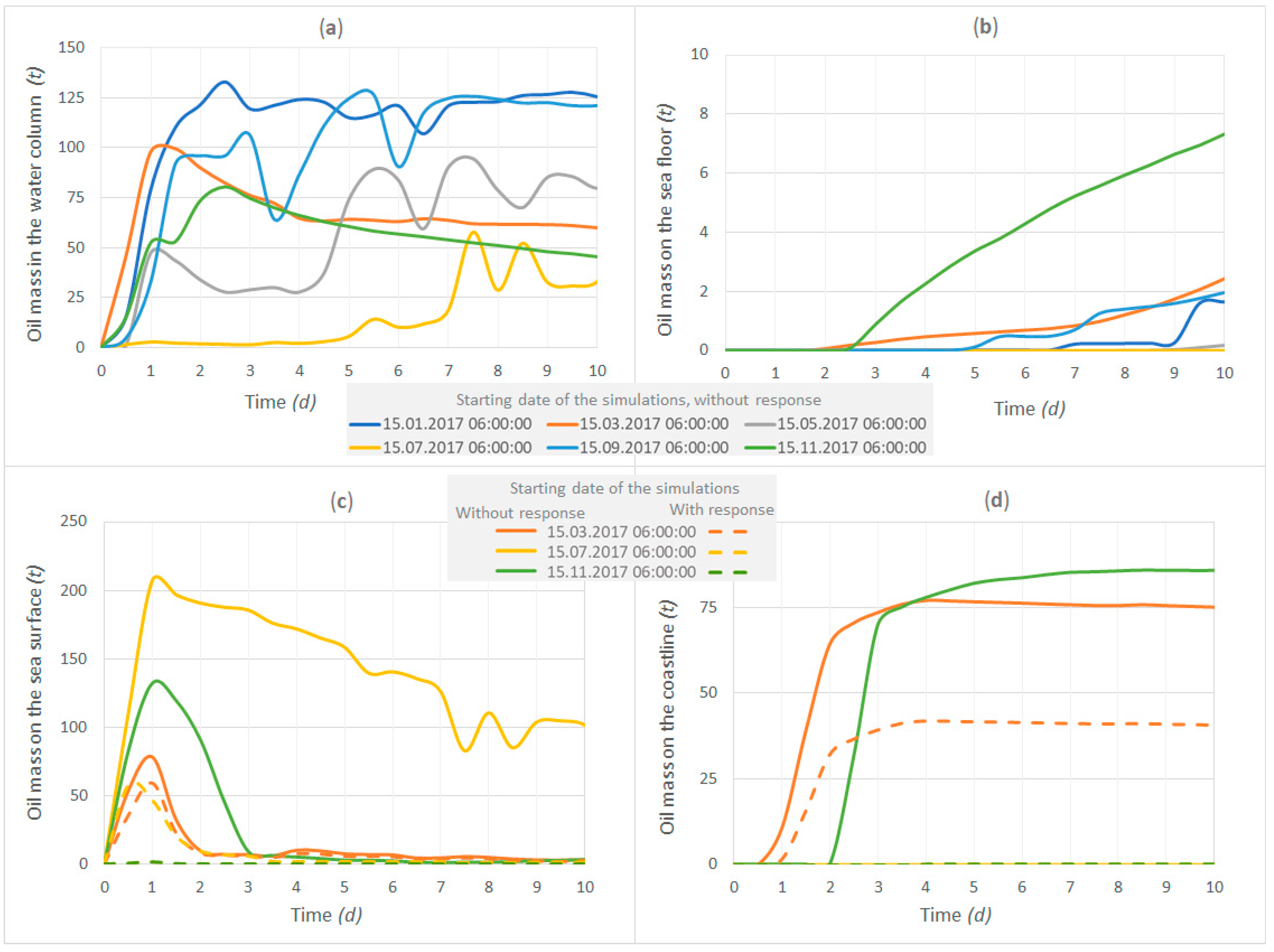
Figure 3a,b shows the temporal trends of the masses of oil in the water column and deposited on the seabed, for six simulations, starting on different dates, in the absence of emergency response. It can be noticed that the curves are dissimilar because of the differences in the meteorological and oceanographic data determining the fate and transport of the oil after the spill, thus justifying the necessity of basing the calculation of the risk for the environment on a large number of metocean conditions.

In Figure 3c,d, the trends of the masses of oil floating on the sea surface and stranded along the coastline are reported for three simulations, considering the absence and the presence of emergency response actions (which correspond to tier 2, as indicated in Table 2). In addition to confirming the strong influence of the starting dates of the simulations on the mass of oil on the sea surface, Figure 3c highlights how emergency response can decrease the amount of floating oil. In fact, while for the simulation starting on 15 March 2017 at 06:00:00 the reduction is slight, for the simulation starting on 15 July 2017 at 06:00:00 the maximum amount of floating oil is reduced by around 75%, and for the simulation starting on 15 November 2017 at 06:00:00 the floating oil is totally eliminated. Hence, the metocean conditions present during the simulation time have a major influence also on the effectiveness of emergency response. Similar considerations apply also to Figure 3d, which refers to the amounts of beached oil. Furthermore, Figure 3d highlights the fact that, for the simulation starting on 15 November 2017 06:00:00, the oil slick does not reach the coastline, neither in presence nor in absence of emergency response. In fact, for this simulation the action of the winds and of the currents pushes the oil slick into the open sea. The vertical dotted line in Figure 3a–d refers to the time at which the oil mass values m_c,i,j were taken for obtaining the F(m_c) risk curves. Since spill T5 has a duration of 2 h, for this spill, the reference time corresponds to 5.08 d. For instance, from Figure 3a, it can be derived that m_watcol, _{T5, 15 January 2017 06:00:00} = 114.8 t, m_watcol, _{T5, 15 March 2017 06:00:00} = 64.1 t, m_watcol, _{T5, 15 May 2017 06:00:00} = 74.2 t, m_watcol, _{T5, 15 July 2017 06:00:00} = 5.6 t, m_watcol, _{T5, 15 September 2017 06:00:00} = 124.3 t, m_watcol, _{T5, 15 November 2017 06:00:00} = 60.4 t.

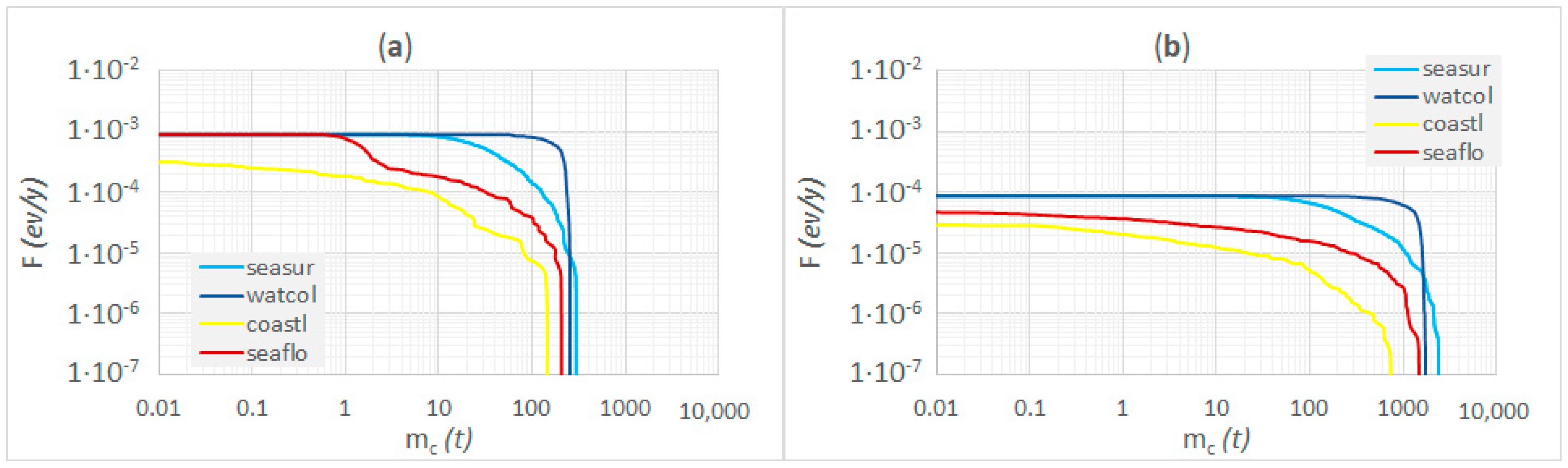
Figure 4 and Figure 5 report some examples of the results obtained in the calculation of the risk indexes for the case study. In particular, Figure 4 shows the F(m_c) curves of spills S10 and T3 in the absence of an emergency response. The figures also evidence how the different compartments are impacted by the oil spill.

From each curve of Figure 4, by applying Equation (4), the yearly expected mass of oil in the corresponding compartment can be obtained, as explained in Section 4. For instance, the simulation of Spill S10 on the different starting dates j (i.e., in different metocean condition j = 1, …, 230) cause a number N_sim = 230 of different values of the mass of oil floating on the sea surface (at the chosen reference time) m_seasur,S10,j, ranging from 2.5 t (if the spill occurs on date j = 28 January 2016 14:00) to 296.0 t (if the spill occurs on date j = 2 June 2013 12:00). Since Equation (2) provides for each starting date an occurrence probability P_met = 0.002 and the frequency of spill S10 f_spill,S10 corresponds to 9.10 × 10⁻⁴ ev/y (as reported in Table 2), by applying Equation (3) the frequency of spill S10 in each metocean condition f_met,j = 3.96 × 10⁻⁶ ev/y can be obtained. 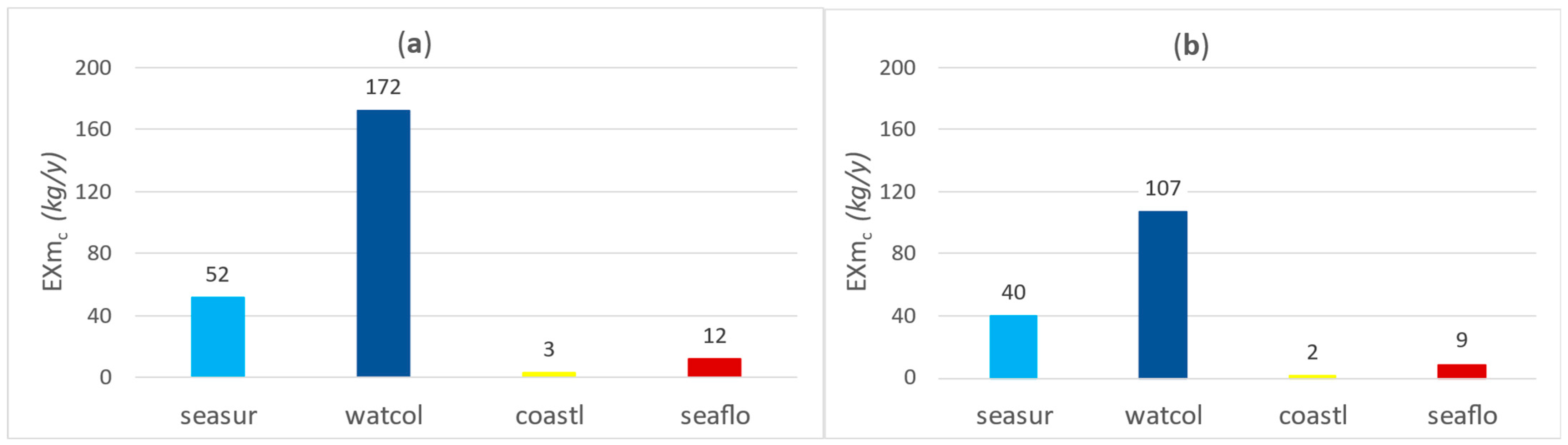Hence, this value represents also the occurrence frequency of each m_seasur,S10,j value. By applying Equation (4), the mass of oil floating on the sea surface yearly expected as a consequence of spill S10 can be calculated, obtaining Exm_sesdurf = 52 kg/y.

By means of this procedure, the amounts of oil yearly expected in all the marine compartments, EXm_c, were obtained for the spills S10 and T3, as reported in Figure 5.

Figure 4a shows that the maximum value of the cumulated frequency, F, for the curves referring to the sea surface, the water column, and the seabed is the same, being equal to 9.1 × 10⁻⁴ ev/y, which is the occurrence frequency of spill S10, as reported in Table 1. Differently, the maximum value of F for the curve referring to the coastline (3.0 × 10⁻⁴ ev/y) is lower. This means that spill S10, which is a subsea release, always results in the contamination of the sea surface, of the water column, and of the sea bottom. However, in some metocean situations, the oil is drifted off the coast by the winds and the currents, so that no oil beaches along the shoreline. Actually, the stranding of the oil occurs in metocean conditions having an overall probability of occurrence expressed by the ratio of the maximum value of F(m_coastl) with respect to the spill frequency, that results equal to about 0.33.

Similarly, Figure 4b shows that when spill T3 is considered, which is a topside release, the metocean circumstances causing the deposition of the oil on the seabed have an overall occurrence probability of about 0.51, while the probability of those resulting in the stranding of the oil is of about 0.33. As expected, the sea surface and the underlying water column are affected by the spill in all metocean conditions.

In general, in case of topside spills, it is possible that in specific metocean data, both the seafloor and the coastline are not impacted by the oil, while, when subsea spills take place in shallow water, as in the case study, the seabed is always affected.

Comparing Figure 4a,b, it is evident that the cumulated frequencies of spill S10 are about one order of magnitude higher that those corresponding to spill T3. However, when looking at the maximum amounts of oil expected in the different sea compartments (i.e., at the maximum values on the x-axis of the plots), these are one order of magnitude higher for spill T3, ranging from 750 t (for the seafloor) to 2500 t (for the sea surface), with respect to spill S10, for which they are between 200 t and 300 t for all the sea compartments. These differences directly derive from the differences in the occurrence frequencies and in the masses of oil released in the two spills, as reported in Table 1. However, Figure 5 shows that the amounts of oil expected per annum in the various sea compartments, EXm_c, are rather similar for the two leakage events, due to the compensation of the spill frequencies and consequences. Thus, while the consequences of spill T3 are on average more severe than those of spill S10, when considering the oil masses expected in the marine compartments, the point value risk indexes result similar for the two spills, being the differences in the risk figures of the two releases within a factor 2, as shown in Figure 5.

These results highlight the usefulness of the environmental risk indexes in comparing the risk of different accidental oil spills in the four marine compartments. Nevertheless, it should be remarked that the risk indexes should not be used to directly compare the risk of a given spill to different sea compartments. Actually, the damage of the oil to the ecological resources is utterly different in the different compartments, so that the ultimate consequences of the oil contamination have to be assessed separately for the sea surface, the water column, the coastline, and the seabed, as confirmed by the procedures proposed by all the OSRA methods available in the literature addressing more than one compartment [23,38].

The above defined risk indexes can be used also to assess the effectiveness of additional safety barriers installed on an offshore facility. In general terms, risk reduction can be achieved by means of preventive measures, reducing the occurrence frequency of the spill events, and by protective measures, reducing the outflow rate and/or the duration of the spill, so to cut down the amount of oil released to the seawater. Since it is widely acknowledged that preventive measures, causing the reduction in spill frequencies, must be given priority [53,88], accounting for the spill frequencies in the risk indexes results of extreme importance. As shown in Figure 4 and Figure 5, the risk indexes defined in the present approach are able to capture the role of the spill frequencies, which are not taken into account by the OSRA methods focusing only on the evaluation of the effects of the spills.

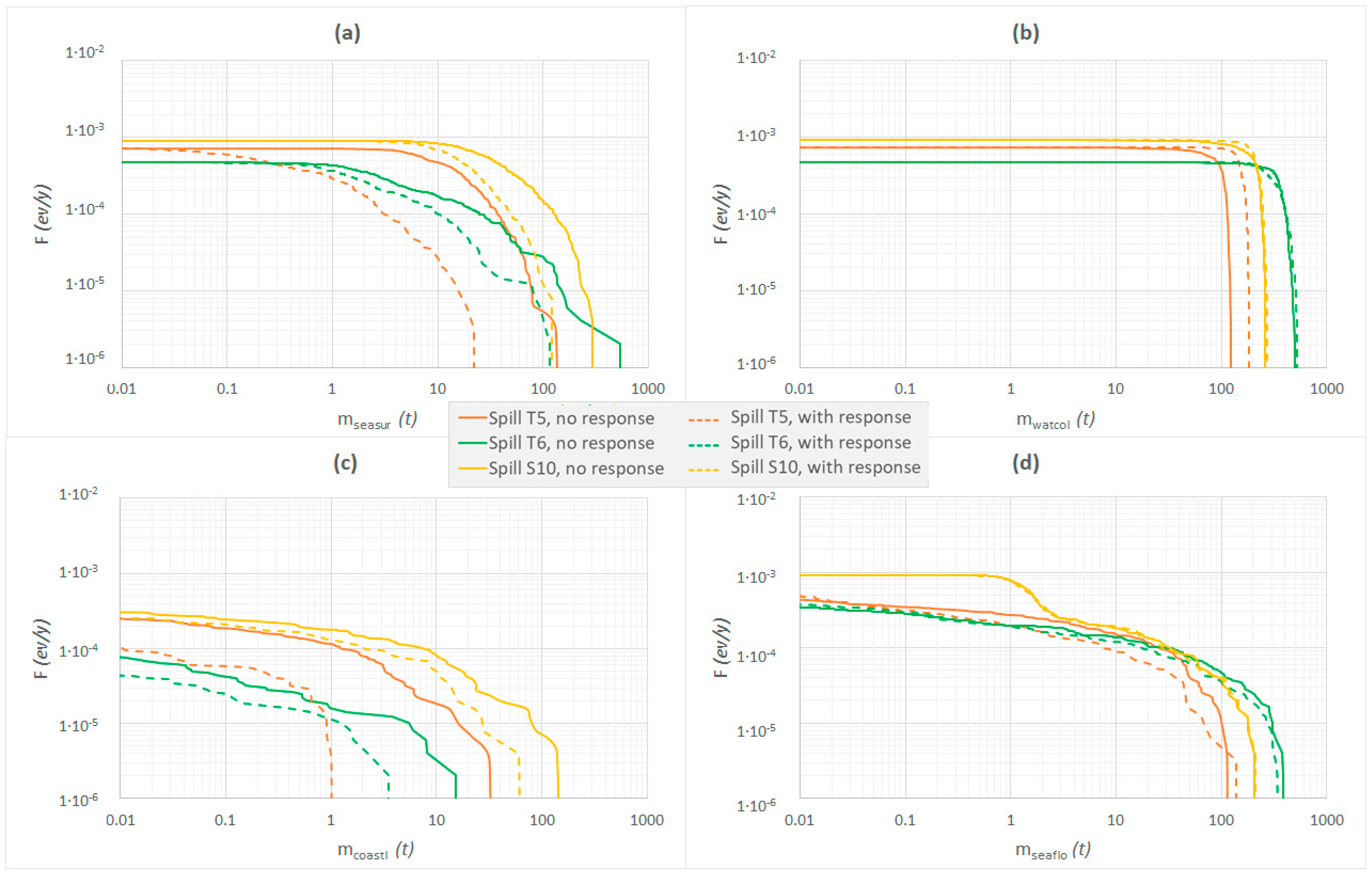
Emergency response measures, as those listed in Table 2, contribute to mitigate the spill consequences. The risk indexes defined in the present approach are suitable to highlight also this influence. Figure 6 reports the F(m_c) curves evaluated both in the presence and in the absence of emergency response for the accidental events assigned to tier 2 response (i.e., spills T5, T6, and S10, as reported in Table 2).

Figure 6a,c shows that, as expected, for all the spills considered, the emergency actions reduce the risk to the sea surface and the coastline. The maximum amounts of oil on the sea surface and beached along the coastline considerably decrease for all the spills. For instance, in the case of spill T5, the maximum mass of oil on the sea surface reported in Figure 6a is reduced from more than 500 t to 120 t, whereas the maximum amount of stranded oil decreases from 32 t to 1 t. Moreover, it can be noticed that, in the F(m_coastl) curves reported in Figure 6c, the maximum values of both the beached oil mass and the cumulated frequency decreases for all the spills. For instance, in case of spill T5 the maximum value of the cumulated frequency is reduced from 2.5 × 10⁻⁴ ev/y to 1.1 × 10⁻⁴ ev/y, highlighting that the combined action of mechanical recovery and spraying of dispersants, which are the remediation strategies adopted in the tier 2 emergency response, halves the probability of oiling the shoreline.

Differently, the comparison of Figure 6b,d shows that the presence of emergency response measures induces only minor changes in the F(m_c) curves referring to the water column and to the seabed. Actually, for spills S10 and T6 the curves in the absence and in the presence of emergency response are nearly overlapped both for the water column and for the seafloor. Instead, for spill T5, the maximum mass of oil impacting the water column results even higher when considering emergency response. This may be reasonably explained keeping in mind that the application of dispersants on the slick, differently from mechanical recovery, does not remove the oil from the sea, rather it transfers the contamination—and thus the risk—from the sea surface to the water column [89,90]. Nevertheless, since the oil can persist on the sea surface for long times (e.g., several days or even weeks), while in the water column it is usually diluted to negligible concentrations within few hours, usually the spraying of dispersants is deemed bringing a considerable net benefit to the marine environment [82,91,92]. When emergency response actions are deployed for spill T5, as a consequence of the increase in the maximum mass of oil in the water column, the maximum mass of oil depositing on the seafloor increases too, as shown in Figure 6d. However, it can be observed that, overall, emergency interventions reduce the cumulated frequency values of oil deposited on the sea bottom.

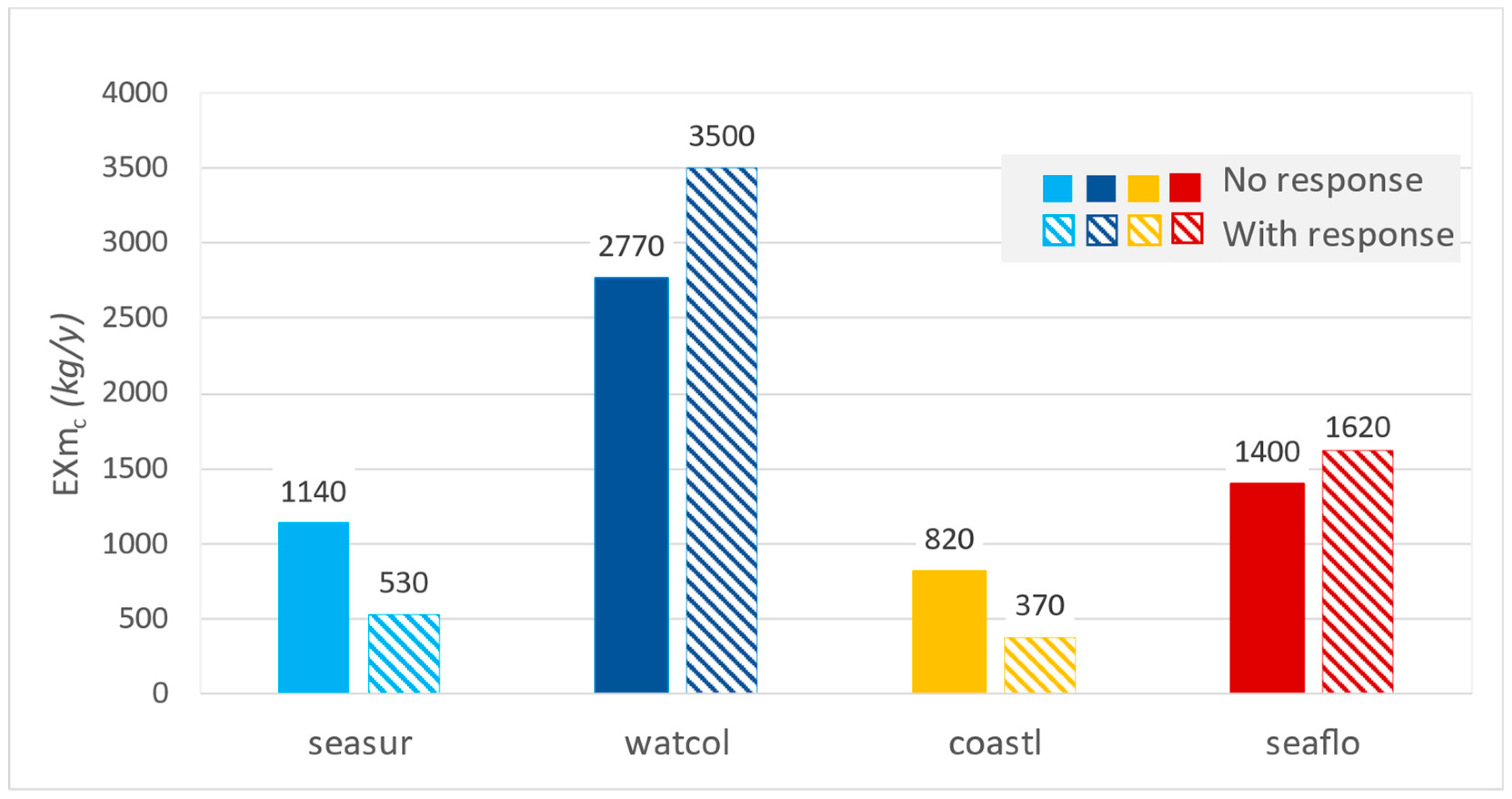
A further insight concerning the influence of emergency response on the environmental risk indexes is achieved by comparing the masses of oil expected each year in the different marine compartments, EXm_c, evaluated in the presence and in the absence of emergency response. Figure 7 reports the results obtained for the entire facility, considering all the 18 oil spills which can occur on the Prudence FPSO, as listed in Table 1.

Figure 7 shows that the masses of oil annually expected on the sea surface and along the coastline are more than halved by emergency response actions, while those impacting the water column and the seabed increase by +21% and +13%, respectively. This result was expected, since the beaching of the oil occurs when the slick floating on the sea surface reaches the coastline, thus a reduction in the amount of oil in the slick reasonably reduces the mass oil that can beach. Similarly, since the deposition of oil on the seafloor derives from the oil entrained in the water column, which sinks by gravity and finally settles down on the sea bottom [73], an increase in the oil present in the water column turns out in an increase in the oil affecting the sea bottom.

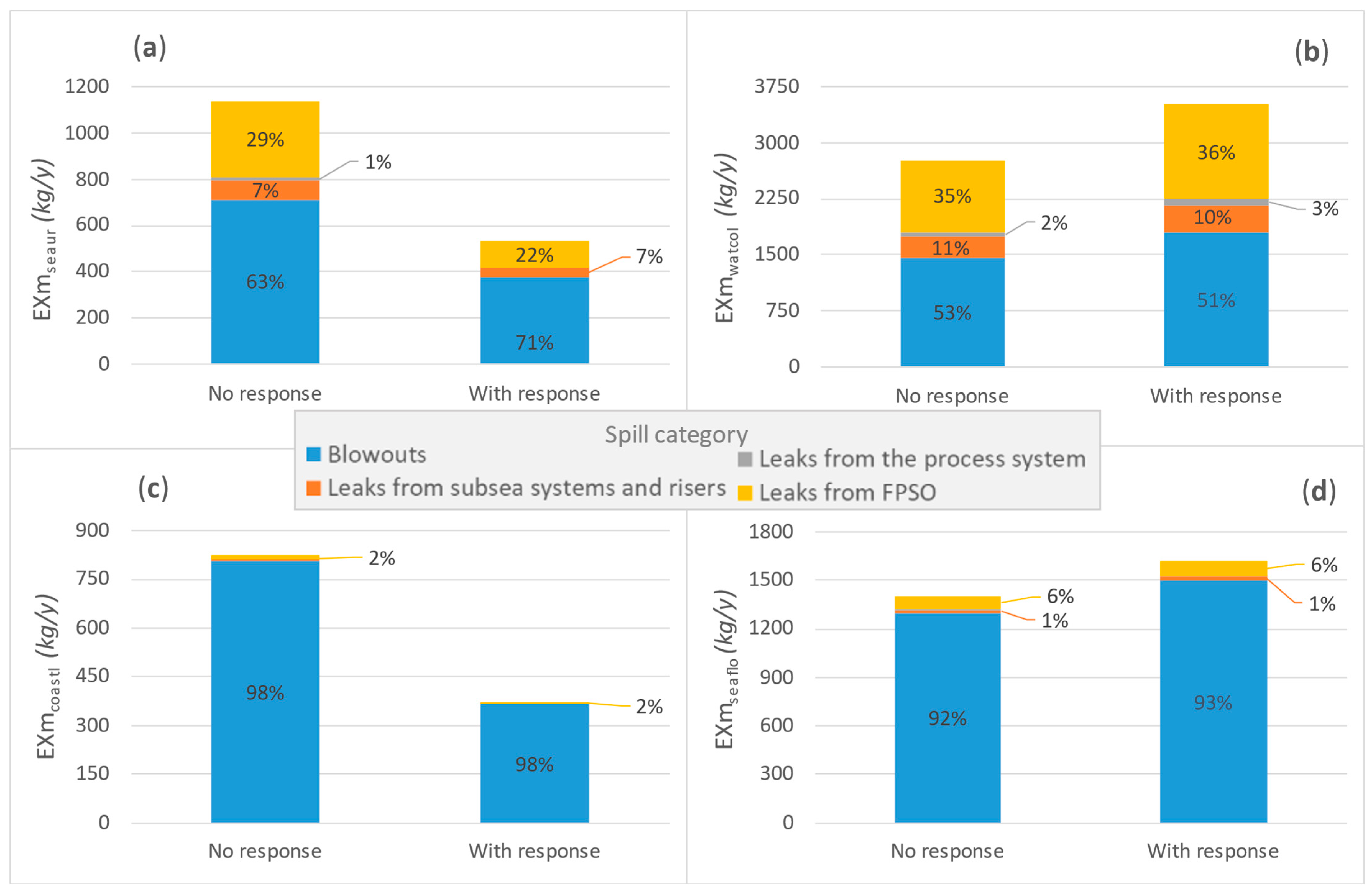
As reported in Table 1, the loss of containment events associated to the Prudence FPSO are grouped in four spill categories, defined on the basis of the system affected by the spill. Figure 8 shows the percentage contribution of each spill class to the masses of oil annually expected in the different sea compartments when considering the entire set of spills.

Figure 8c,d highlights that the masses of oil yearly expected to be deposited along the shoreline and on the seabed derive almost entirely from blowouts, which provide a contribution ranging from 92% to 98% of the total mass. The role of blowouts is rather important also when considering the sea surface (for which the contribution reaches 71%, as shown in Figure 8a) and the water column (for which the contribution is in the range 51% ÷ 53%, as shown in Figure 8b). However, in the latter compartments, also the leaks from the FPSO considerably influence the annual expected amount of oil. Differently, the contributions of the releases from the subsea systems and risers play a minor part in the oil affecting the sea surface and the water column, having a negligible importance when considering the impact on the seafloor and on the coastline. Finally, the influence of the spills from the process system is minor for all the marine compartments.

It can also be noticed that, differently from the expected oil masses, the percentage contributions of the oil spill categories to the overall risk are not affected by the presence of emergency response interventions, having rather similar values in the absence and in the presence of emergency response whatever the sea compartment.

The information presented in Figure 8 is useful to address the introduction of further safety barriers and/or to improve the effectiveness of the existing ones. Actually, the results clearly show that safety measures addressing the process system would have a negligible effect on the risk of the whole installation, while additional safety barriers preventing blowouts could significantly reduce the risk figures of the Prudence FPSO.

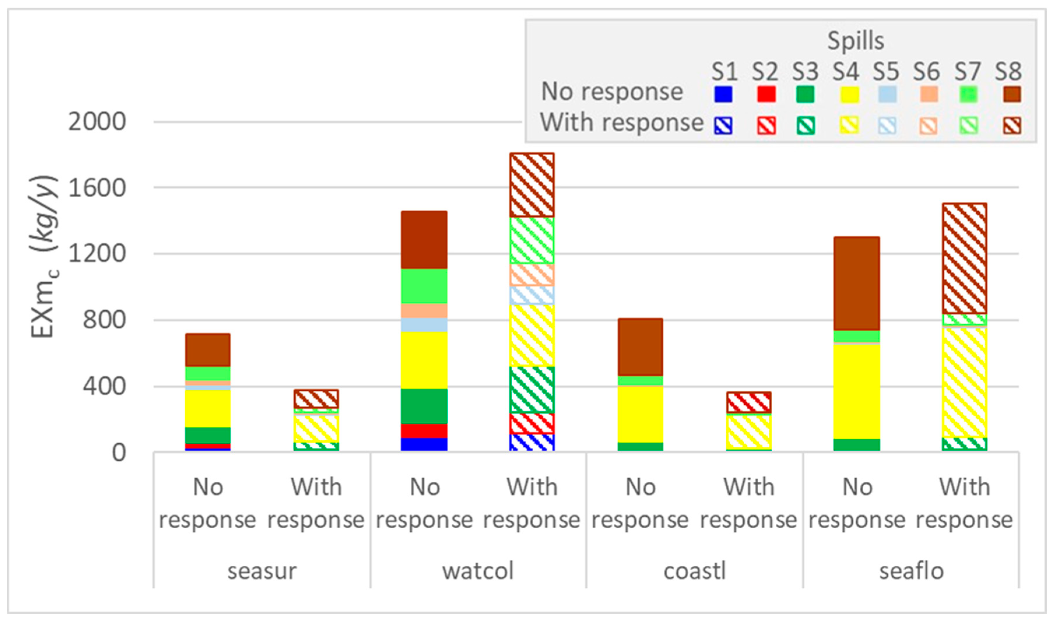
The support provided by the above defined risk indexes to decision-making addressing the design of safety barriers can be even higher, if the level of detail of the risk results is increased. As an example, Figure 9 shows the masses of oil expected to affect yearly the various marine compartments, considering separately spills S1 to S8, i.e., the leakage events related to blowouts. The annual expected amounts of oil were obtained for each of these spills both in the absence and in the presence of emergency response, considering a tier 3 response, as indicated in Table 2.

Looking at Figure 9, it is evident that the risk values of the spills of the couples S1 and S5, S2 and S6, S3 and S7, S4 and S8, are rather similar. This similarity was expected, since the spill volumes and the spill frequencies present minor differences within each couple, as evidenced in Table 1.

Furthermore, Figure 9 shows that for all the blowout spills, emergency response actions cause a relevant risk reduction for the sea surface and the coastline, even if the risk is transferred to the water column and the sea bottom, determining a minor increase in the amounts of oil per annum expected in the latter compartments. The subsea injection of dispersants, which cannot be simulated by the OSCAR software, as explained before, would enhance even more the risk transfer between the marine compartments.

It can also be noticed that spills S4 and S8, which are assumed to last for 50 days, as reported in Table 1, provide the most relevant contributions to the risk indexes associated to blowouts. Thus, actions aimed at risk reduction should give priority to the prevention and mitigation of these spills, since measures addressing the other blowout events would have a minor effect on the risk of this class of spillages. Thus, the usefulness of the risk indexes defined in orienting the implementation of safety actions is confirmed.

The results reported in Figure 9 also evidence that the annual amount of oil expected to reach the seafloor could be relevant in shallow waters, as those characterizing the Prudence oil field. Even if a specific assessment is needed to understand the environmental damage caused by the oil impacting the seabed, the risk results obtained confirm the need to include the sea bottom in the overall assessment of the risk to the environment posed by oil spills.

6. Discussion

A first important remark concerns the importance of the developed approach in the perspective of the application of the provisions of Directive 2013/30/EU. As shown in the previous section, the novel methodology allows for complying with the prescriptions of the Directive. In particular, the method developed provides the risk indexes in the absence and in the presence of emergency response systems, as explicitly required by the Directive, thus allowing for the quantification of the effectiveness of the contingency actions undertaken to combat oil spills. Actually, the method supports the quantitative assessment of the risk reduction due to different response strategies (i.e., mechanical recovery, application of dispersants, and in situ burning), also considering specific local factors that introduce differences in the deployment of each strategy (e.g., in regard to the location, type, and number of the oil spill response equipment and personnel). As a consequence, it can assist decision makers involved in oil spill contingency planning.

Moreover, the approach allows the comparison of the risk to the environment deriving from different engineering design options of offshore installations. Actually, different technological solutions can be adopted for extracting, processing, and transporting the hydrocarbons (e.g., with respect to the type of offshore structures, the location of the wellheads, the manifolds and risers, the number and types of separators, the number and type of storage vessels, the transfer to the mainland of the hydrocarbons, etc.). The new method is applicable whatever the design configuration of the installation. In fact, the different failure rates, failure modes, and release inventories deriving from different technology concepts and operating conditions may be considered in the application of the method, resulting in different occurrence frequencies and different source terms of the oil spills, and, consequently, in different values of the risk indexes. Thus, the method may support risk-based decision making for the identification of the preferred design option.

It should also be remarked that the new OSRA approach, though applied in the present study only to oil and gas facilities, can be easily extended to oil tankers and, more generally, to all the sources potentially releasing crude oil and hydrocarbons into the marine environment (e.g., oil reservoirs—even in presence of enhanced oil recovery), fixed installations along the coasts, sealines, ships fueled with oil products). This feature is extremely valuable, since it allows for calculating the risk to the environment of a specific sea area, taking into account all the anthropic activities from which oil spills may derive. In fact, using the same indexes for expressing the risk to the environment provides a complete risk figure, as well as an immediate comparison of the contribution of each oil spill source to the overall risk. Thus, the approach developed supports the identification of the main risk sources in a region of interest and represents an effective guide to risk mitigation actions.

It has to be pointed out that while for the Prudence FPSO case study the OSCAR software was used, the new OSRA method does not require the adoption of the OSCAR code for the estimation of the fate and transport of the oil. In fact, any other model for the consequence assessment of oil spills providing the temporal trend of the masses of oil in the marine compartments and capable of taking into account the influence of emergency response can be used. Consequently, any advance in oil spill modeling, and in particular in the simulation of the response techniques which can be deployed to combat a major oil spillage, can be easily included in the method, contributing to a more realistic assessment of the amounts of oil in the sea compartments and, hence, of the risk of environmental contamination caused by oil spills. Intuitively, the applicability limit of the software tool selected for the consequence assessment of the oil spills becomes an applicability limit of the OSRA procedure too. Firstly, the software has to be applicable to the sea area to be considered. For instance, if the new procedure has to be used in the Arctic, an oil spill code capable of simulating the fate and trajectory of the oil in ice-covered water is necessary. Secondly, the oil/oil product spilled has to be present in the oil database of the software adopted for the consequence assessment of the oil spills, or at least to be similar to one of the oils included in the database. Thirdly, the software should be able to consider the amount, rate, and duration of the oil spills to be simulated. For instance, while in the OSCAR software there is no upper limit to the amount of oil spilled, the use of this code is optimal for spills over 5 tons. In fact, all oil spills of the Prudence FPSO case study comply with this requirement. Lastly, the oil spill code needs to be able to model the response strategies of the oil spill contingency plan. While most codes (and among them, the OSCAR software) can take into account mechanical recovery, application of dispersants, and in situ burning, the simulation of the subsea injection of dispersants is not yet possible, although specific studies are currently undertaken for the inclusion of this strategy among the response options [93].

Notably, in order to obtain robust risk indexes orienting the aforementioned decision-making processes, curbing the amplification of uncertainty in the estimation of the risk of oil spills is crucial. For this reason, the novel risk indexes assume the mass balance results of the stochastic simulations of the oil spilled at sea as the consequences of the spill, since the oil masses in the marine compartments are affected only by the features of the spill and by the local metocean conditions, but not by the ecological resources in the area.

However, this strong point of the method also represents its limitation. In fact, this approach does not assess the impact on and the damage to the ecological species and the natural habitats in the region affected by the oil spills. Actually, exposure- and damage-based methods are capable of estimating the effects of oil spills on marine and coastal wildlife and plants. This information is essential for planning wildlife rescue, clean-up, and rehabilitation activities, as well as for the protection and restoration of natural habitats. Hence, the methodology developed, which can be placed between source- and exposure-based methods, requires to be complemented by the application of exposure- and damage-based models. In this sense, it represents a risk screening method providing a preliminary assessment of the risk of environmental contamination.

Nevertheless, the new OSRA method can be applied to seas where currently exposure- and damage-based risk procedures cannot be used due to the lack of data on the ecological components. This issue is of particular importance, since the description of the natural resources has been started only recently and is not yet available in several regions, currently impeding the application in these areas of methods requiring the assessment of exposure and damage. Even in countries that have always been at the cutting-edge of the consequence analysis of oil spills, the limited availability and poor quality of the data on the ecological components (whether the species have been mapped, what is their geographical distribution and their temporal presence) is still a critical issue (e.g., in Norway [52]).

It should be remarked that the oil spill occurrence frequencies and the spatio-temporal distribution of the oil in the marine compartments, which are necessary for the calculation of the new risk indexes, may well be used, in a following step, to feed exposure- and damage-based models. Thus, considering the rapid progress of the mapping of the ecological species in more and more marine areas, in perspective the results of the present approach are of value also for the application of exposure- and damage-based oil spill risk models, that may be applied as a follow-up to the present methodology, to gather a more detailed picture of the impact of oil spills on the different environmental compartments. The results of the latter approaches can be further processed for predicting the expected costs of the oil spills, up to the clean-up and restoration of the natural components damaged by the oil [94,95].

7. Conclusions

The methodology developed provides a novel comprehensive approach for the preliminary quantitative analysis of the risk of environmental contamination caused by oil spills from offshore facilities. The method allows complying with the provisions of Directive 2013/30/EU concerning the analysis of the risk to the marine compartments. The new risk indexes are able to provide a direct quantification of the mitigation introduced by emergency response systems, as explicitly required by the Directive, thus supporting the development of contingency response plans to combat oil spills. The new indexes are also effective in supporting the comparison of the risk to the environment deriving from alternative engineering design options of oil and gas installations. The novel OSRA method thus overcomes the five main limitations of the available methodologies evidenced in Section 2, and can be applied also to seas and geographical areas where currently exposure- and damage-based risk procedures cannot be adopted, due to the lack of data on the ecological components. In addition, the new approach, though described in the present study only with reference to oil and gas facilities, can be easily extended to oil tankers and, more generally, to all the sources potentially releasing oil and oil products into the marine environment (e.g., fixed installations along the coasts, sealines, ships fueled with oil products). This feature is crucial to the calculation of the risk of environmental contamination caused by oil spills in a specific sea area, which has to take into account all the installations and anthropic activities from which oil spills impacting the area can derive.

Therefore, the methodology described in the present study contributes in providing the oil and gas industry and the competent authorities with a thorough picture of the risk to the environment caused by oil spills, based on quantitative data. The risk figures obtained may give effective support for the implementation of exposure- and damage-based models, as well as the definition of oil spill risk reduction actions, in order to enhance the environmental protection of the sea.