Article

Fused Geophysical–Contrastive Learning Model for CYGNSS-Based Sea Surface Wind Speed Retrieval in Typhoon Regions


1
College of Information Technology, Shanghai Ocean University, Shanghai 201306, China
2
Shanghai Marine Intelligent Information and Navigation Remote Sensing Engineering Technology Research Center, Shanghai 201306, China
3
College of Foreign Languages, Shanghai Ocean University, Shanghai 201306, China
4
Guangxi Meteorological Observatory, Nanning 530022, China
5
School of Geodesy and Geomatics, Wuhan University, Wuhan 430079, China
*
Author to whom correspondence should be addressed.
J. Mar. Sci. Eng. 2026, 14(2), 208; https://doi.org/10.3390/jmse14020208
Submission received: 22 December 2025 / Revised: 14 January 2026 / Accepted: 16 January 2026 / Published: 20 January 2026
(This article belongs to the Section Physical Oceanography)

Abstract

Global Navigation Satellite System Reflectometry (GNSS-R) provides a vital means for sea surface wind speed retrieval, yet its application under extreme typhoon conditions remains challenging. Conventional geophysical models (GMFs) saturate in high wind speed regimes (>20 m/s), and deep learning models (e.g., CNNs) are constrained by data sparsity and feature complexity in typhoon environments. To address these issues, we propose a Comparative Learning method of CNN-Transformer with GMF fusion (CLCTG). The CNN branch extracts local coupling patterns, the Transformer branch models global dependencies, and Kullback–Leibler (KL) divergence loss is used for contrastive learning to heighten sensitivity to complex typhoon wind fields. The GMF branch serves as a physical reference/anchor in the low- to moderate-wind-speed range (<20 m/s) to guide the learning of data-driven branches and avoid overfitting by any single data-driven path. The adaptive fusion branch dynamically reweights the three branch outputs, combining local statistical characteristics to improve performance over approximately 0–30 m/s and extending the range of reliable GNSS-R retrieval from about 20 m/s to about 30 m/s; it should be noted that CLCTG exhibits a performance bottleneck in the extreme >30 m/s range. To further improve high-wind-speed predictions, we introduce environmental features based on their correlation with wind speed; ablation experiments demonstrate that the combined use of environmental parameters and CYGNSS features maximizes overall accuracy. Testing on five typhoons from the Eastern and Western Hemispheres confirms CLCTG’s generalization across diverse geographic contexts, and branch-wise comparisons validate its structural advantages. Buoy observations show peripheral errors below 3 m/s and physically consistent wind speed gradients in the core region. These results indicate that multi-source fusion of CYGNSS and environmental data, coupled with contrastive learning and physical reference, offers a reliable and efficient solution for typhoon wind speed retrieval.

1. Introduction

Typhoons are among the most destructive natural disasters worldwide, and the sea surface wind field is a key element for accurate forecasting of both typhoon intensity and track. Currently, conventional remote-sensing and GMF-based approaches achieve reasonable accuracy in the low- to moderate-wind-speed range (<20 m/s), but a unified benchmark for systematic performance assessment at high wind speeds (>20 m/s) is still lacking, and validation samples are extremely sparse. Although synthetic aperture radar (SAR) has shown potential for polarimetric inversion at high wind speeds [1,2], its limited revisit period makes it difficult to meet the requirements of real-time typhoon monitoring. Exploiting the forward-scattering characteristics of GNSS-R for wind speed retrieval offers a new avenue for high-wind monitoring.
Since Zavorotny and Voronovich proposed the two-dimensional delay–Doppler power model [3,4], researchers have developed various geophysical models based on delay–Doppler map (DDM) observables. In addition, deep-learning methods can be regarded as a data-driven, generalized GMF that, by fusing more input features to mine more complex nonlinear relationships, offers greater flexibility and accuracy for wind speed retrieval.
In 2014, Clarizia et al. [5] constructed a minimum-variance estimator by combining multiple observations, achieving a root-mean-square error (RMSE) of 1.65 m/s in the low- to moderate-wind-speed range. In 2016, Rodriguez et al. [6] used principal component analysis (PCA) to optimize linear combination coefficients, but the overall RMSE exceeded 4 m/s when wind speed exceeded 20 m/s. In 2018, Ruf et al. [7] developed the Fully Developed Seas (FDS) GMF for medium-to-low winds (RMSE ≈ 2 m/s) and the Young Seas/Limited Fetch (YSLF) GMF for hurricane conditions (high-wind RMSE ≈ 6.5 m/s). In 2021, Pascual et al. [8] further introduced significant wave height (SWH) to construct a two-dimensional lookup table, reducing the retrieval RMSE to 1.19 m/s. These studies demonstrate the reliability of GNSS-R at low-to-moderate wind speeds, but traditional GMFs typically show marked accuracy degradation when wind speed exceeds 20 m/s due to increased complexity in sea surface scattering mechanisms.
In recent years, deep learning—viewed as a data-driven generalized GMF—has shown advantages in handling nonlinear relationships. Architectures such as fully connected networks (FCNs) [9,10,11,12], convolutional neural networks (CNNs) [13], and Transformers [14] have been widely applied. In 2022, Asgarimehr et al. [15] proposed CyGNSSnet, which reduced RMSE by approximately 28% relative to traditional methods. Also in 2022, Guo et al. [16] introduced an improved CNN (MCNN), achieving RMSEs of 1.46 m/s and 2.97 m/s in the 0–12 m/s and 12–25 m/s ranges, respectively. In 2023, Lu et al. [17] used a CNN–LSTM to capture spatiotemporal features and reported an RMSE of 1.34 m/s over the 0–30 m/s range. In 2024, Du et al. [18] further reduced errors in high-wind regimes using a residual fully convolutional network (RFCN) and fine-tuning strategies. Their fine-tuned RFCN (FT_RFCN) achieved RMSEs of 1.031 m/s for 0–30 m/s and 3.283 m/s for >20 m/s. Nevertheless, despite their flexibility in function approximation, neural networks remain limited under extreme conditions by: (i) scarcity of training samples; (ii) potential distortion due to lack of physical priors; and (iii) insufficient attention to the dynamic evolution of wind fields.
To address these bottlenecks, the CARE framework proposed by Ge et al. [19] demonstrated the potential of contrastive learning to enhance feature representation. However, in typhoon scenarios, the intertwining of extreme winds (>30 m/s) and intense spatiotemporal dynamics (e.g., eyewall structures and spiral rainbands) poses systemic challenges: high-quality validation data in core regions are scarce, conventional physical models may fail, and pure data-driven methods face uncertainty in extrapolating to extreme wind speeds.
Therefore, developing a retrieval method that can synergize physical mechanisms with data-driven strengths, mitigate extreme-sample scarcity, and accurately characterize the dynamic evolution of a typhoon core is a critical gap for improving typhoon monitoring and early-warning capabilities. To address this challenge, this paper proposes a Comparative Learning method that fuses CNN-Transformer models with a GMF (CLCTG). The model is an engineering-oriented, multi-branch hybrid framework designed for extreme typhoon conditions. The framework highlights are as follows:
(1)
Adopt a dual-branch architecture with a CNN branch and a Transformer branch and introduce contrastive learning based on the Kullback–Leibler divergence to align local and global representations under few-sample conditions and enhance generalization capability in high-wind-speed regions;
(2)
Establish a GMF branch as a physical prior reference that is used only in the medium-to-low wind-speed regions where GMF is effective, serving as a physical anchor to guide learning and thereby avoiding enforced reliance on GMF in high-wind-speed regions where it fails;
(3)
Design an uncertainty-based adaptive fusion strategy that dynamically balances between data-driven predictions and the GMF reference to maintain robustness when the physical model locally fails or data uncertainty increases.
The reported performance metrics for the aforementioned models are taken from their original publications; their experimental datasets and reference ground truth differ from those used in this study. This study used CYGNSS data from January 2019 to July 2023 for model training, and several representative typhoon cases were selected for testing (Pacific: SAOLA, YAGI, BEBINC; Atlantic: IDALIA, BERYL). The inversion results of CLCTG were further validated through multi-source comparisons with the U.S. National Centers for Environmental Prediction (NCEP) reanalysis data, CYGNSS L2 (CYL2) product data, the International Best Track Archive for Climate Stewardship (IBTrACS) best-track typhoon data, and in situ buoy measurements from the U.S. National Data Buoy Center (NDBC) in order to comprehensively evaluate its accuracy, robustness, and capability in capturing the dynamic evolution of typhoon wind fields.

2. Datasets and Data Processing

2.1. CYGNSS Dataset

The CYGNSS constellation was successfully deployed on 15 December 2016 [20]. This system comprises eight microsatellites, each with a mass of about 30 kg, operating in a low Earth orbit at an approximate altitude of 520 km and an inclination of 35° [21]. Every satellite carries one right-hand circularly polarized (RHCP) antenna to acquire direct signals from GPS transmitters and two left-hand circularly polarized (LHCP) antennas to capture signals reflected from the ocean or land surfaces. By integrating the all-weather capability of GPS bistatic radar with enhanced spatiotemporal sampling, CYGNSS overcomes the coverage and meteorological constraints inherent in conventional observation methods. The present analysis employed data from the CYGNSS Version 2.1 product [22].
Wind speed retrieval within the CYGNSS framework relies on a key observable known as the DDM. Wind-sensitive geophysical observables, primarily the Normalized Bistatic Radar Cross Section (NBRCS), are derived from the DDM. The NBRCS is computed specifically around the specular point using a window of 3 delay bins and 5 Doppler bins. The theoretical model for the DDM correlation power of GNSS signals scattered from the sea surface [23] is given by
P τ ^ , f ^ g = P T λ 2 4 π 3 A G x , y T σ x , y 0 G x , y R R x , y T 2 R x , y R 2 Λ τ ^ ; x , y 2 S f ^ ; x , y 2 d x   d y
where P τ ^ , f ^ g denotes the coherently processed received power of the scattered signal, P T is the GNSS satellite transmit power; G x , y T and G x , y R represent the antenna gains of the transmitter and receiver, respectively; R x , y T and R x , y R are the distances from the GNSS satellite and the receiver to the mirror reflection point [24]; σ x , y 0 is the NBRCS, which is related to the roughness of the scattering surface; λ is the carrier wavelength of the GNSS satellite signal [3]; Λ τ ^ ; x , y 2 and S f ^ ; x , y 2 are the delay and Doppler spreading functions of the GPS signal; and A defines the integral area over the effective scattering surface for each delay–Doppler cell. The NBRCS ( σ 0 ) is obtained by combining the calibrated bistatic radar cross section with the effective scattering area [25,26,27], calculated as
σ 0 = σ t o t a l A t o t a l = i = 1 N j = 1 M σ τ i , f j i = 1 N j = 1 M A τ i , f j
where σ t o t a l  and A t o t a l  are the aggregate scattering cross-section and effective scattering area within a selected DDM window, with M and N representing the window’s Doppler and delay dimensions, respectively. For CYGNSS, the standard processing uses a window of size M = 5 (Doppler) and N = 3 (delay) centered on the specular point.
This study utilized CYGNSS L2 YSLF (CYL2) data, which provided time-stamped and geolocated mean wind speeds (m/s) and mean square slopes (MSS) at a resolution of 25 × 25 km. Version 3.2 applies the latest GMF/SWH correction method, incorporates additional swell correction under low wind speed conditions, and features improved quality control, delivering more accurate and reliable wind speed estimates. As the most recent release available for model validation, it enables verification of generalization capability under new algorithms and annotations. Therefore, CYL2 v3.2 data was selected as one of the datasets for accuracy verification.

2.2. ECMWF ERA5 Dataset

The European Centre for Medium-Range Weather Forecasts (ECMWF) ERA5 reanalysis dataset combines model data with observations from diverse sources to generate estimates of atmospheric states, making it one of the most widely used climate datasets [28]. To enhance sensitivity to high wind speed retrieval, four environmental parameters were selected: mean sea level pressure (MSL), sea surface temperature (SST), total precipitation (TP), and significant wave height of combined wind waves and swell (SWH). The spatial–temporal resolutions for MSL, TP, and SST are 1 h and 0.25°, while SWH has a resolution of 1 h and 0.5°, both in Coordinated Universal Time (UTC). First, the spatial resolutions of MSL, TP, and SST are resampled to 0.5° to align with SWH. These four environmental parameters are spatially matched with the corresponding CYGNSS data using a grid-matching method.

2.3. NCEP Dataset

NCEP dataset, jointly developed by NCEP and the National Center for Atmospheric Research (NCAR), is one of the most important global atmospheric reanalysis datasets. It employs a cutting-edge global system for data assimilation, supported by an extensive repository of information. Through rigorous quality control procedures, it incorporates observational data derived from a multitude of sources such as ground-based stations, maritime vessels, radiosondes, weather balloons, aircraft, and satellite platforms, forming a comprehensive dataset characterized by rich content, extensive coverage, and a long time span. In particular, the accuracy of NCEP data in high wind speed conditions is superior, providing reliable support for high wind speed retrieval [7,29,30]. To match the spatial resolution of ERA5 data, this study adopted NCEP wind speed data at 10 m above sea level, with a spatial–temporal resolution of 1 h and 0.5°.

2.4. IBTrACS Dataset

IBTrACS is the most comprehensive global repository for tropical cyclone data. This project integrates recent and historical tropical cyclone records from multiple agencies to create a unified, publicly accessible best-track dataset, facilitating cross-agency comparisons. IBTrACS is collaboratively developed by Regional Specialized Meteorological Centers (RSMCs) under the World Meteorological Organization (WMO) and other global organizations and individuals. In this study, the typhoon trajectory boundaries (latitude and longitude ranges) were determined using IBTrACS data, and typhoon center wind speeds were employed to validate the model’s retrieval results.

2.5. NDBC Dataset

NDBC, affiliated with the National Oceanic and Atmospheric Administration (NOAA), manages observational data collected from approximately 100 moored buoys and Coastal-Marine Automated Network (C-MAN) stations. This includes 55 Tropical Atmosphere Ocean (TAO) buoys deployed and maintained in the equatorial Pacific Ocean, covering latitudes from 9° N to 8° S and longitudes from 95° W to 165° E. Measured wind speed data from NDBC buoys located in typhoon-affected regions were utilized to validate the model’s retrieval results for Western Hemisphere typhoon areas.

3. Method

In this section, the experimental dataset is constructed using the data sources described in Section 2, and the CLCTG model is proposed. The SHAP (SHapley Additive exPlanations) interpreter is further employed to investigate the contributions of input features and their physical mechanisms.

3.1. Data Preprocessing

Prior to dataset construction, data preprocessing was performed. This study adopted NCEP wind speeds as reference wind speeds and spatially matched them with CYGNSS data through a grid-matching method to achieve a spatiotemporal resolution of 0.5° × 0.5° × 1 h. Unlike commonly used linear interpolation, grid-matching directly projects all observations onto fixed grid points: different sources (e.g., CYGNSS, NCEP) correspond to the same grid center value or nearest-neighbor value. This avoids excessive smoothing or distortion of wind speeds in high-gradient regions (e.g., near typhoon eyewalls) while ensuring multi-source data consistency at identical grid points. The following quality filters were applied to the matched data:
CYGNSS Filter Criteria:
  • The quality control (QC) flag in the CYGNSS L1 dataset uses bit combinations to flag various data quality issues. Records identified by the following labels are excluded according to standard processing protocols.
    (a)
    poor_overall_quality: Poor overall quality (including attitude errors, CRC failure, RFI, etc.);
    (b)
    s_band_powere d_up: S-band transmitter powered on;
    (c)
    small_sc_attitude_err: Minor attitude errors (roll 1–30°, pitch 1–10°, yaw 1–5°);
    (d)
    large_sc_attitude_err: Major attitude errors (roll ≥ 30°, pitch ≥ 10°, yaw ≥ 5°).
  • The data selection requires both the wind speed matching value and the CYGNSS observation data to be positive.
  • A range corrected gain (RCG) value greater than 10 constitutes a criterion for data removal, with its formal definition and physical meaning provided in reference [31].
  • The incident angle of the satellite antenna is less than 60°.
  • The specular reflection point is on the sea.
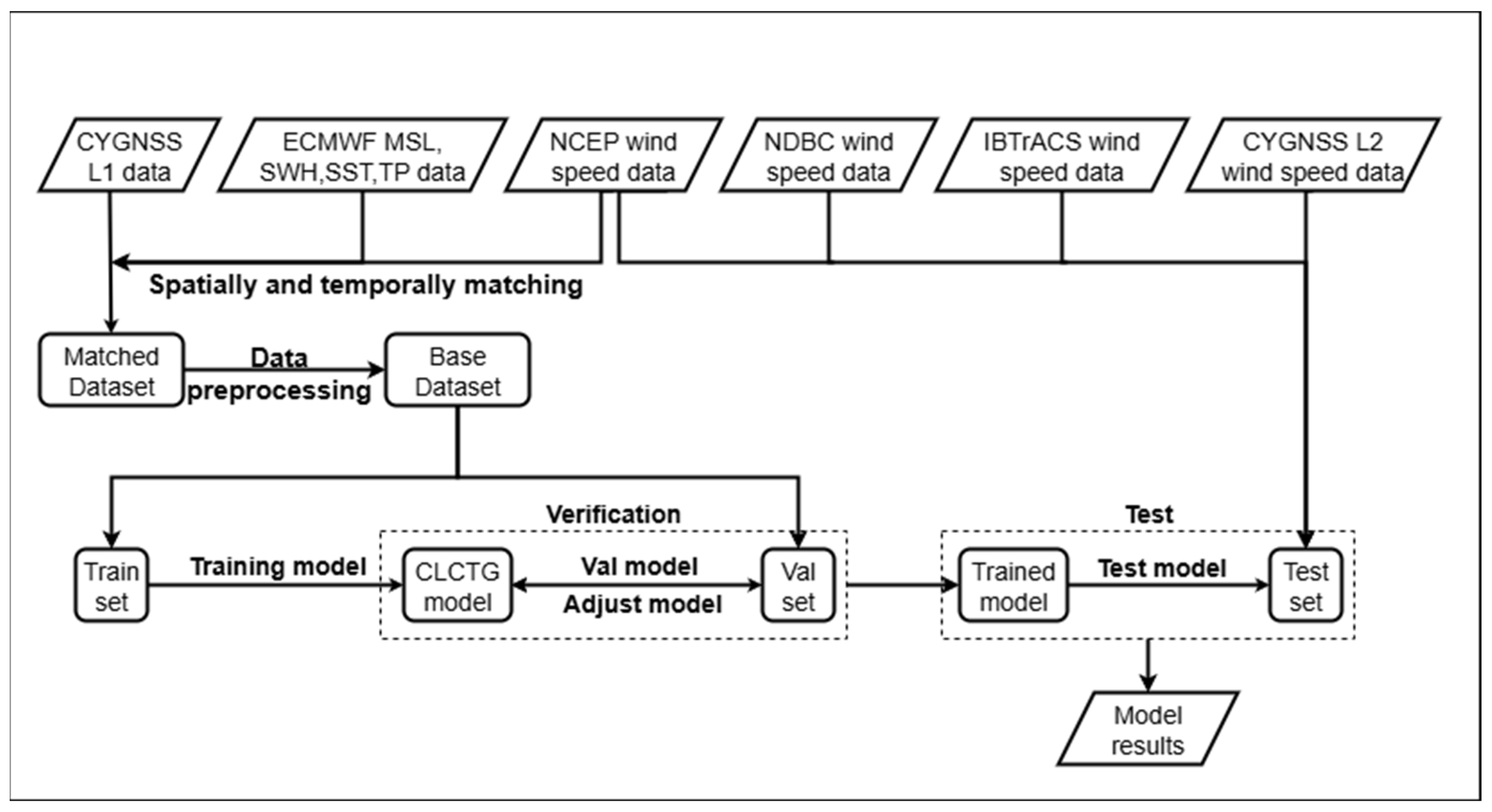
Subsequently, the filtered data were further grid-matched with ERA5 environmental parameters (MSL, SST, TP, and SWH) at the same spatiotemporal resolution (0.5° × 0.5° × 1 h). Entries with incomplete environmental parameters were discarded. Finally, the fully matched dataset was partitioned into training, validation, and test sets, with the workflow illustrated in Figure 1.

3.2. Building an Experimental Dataset

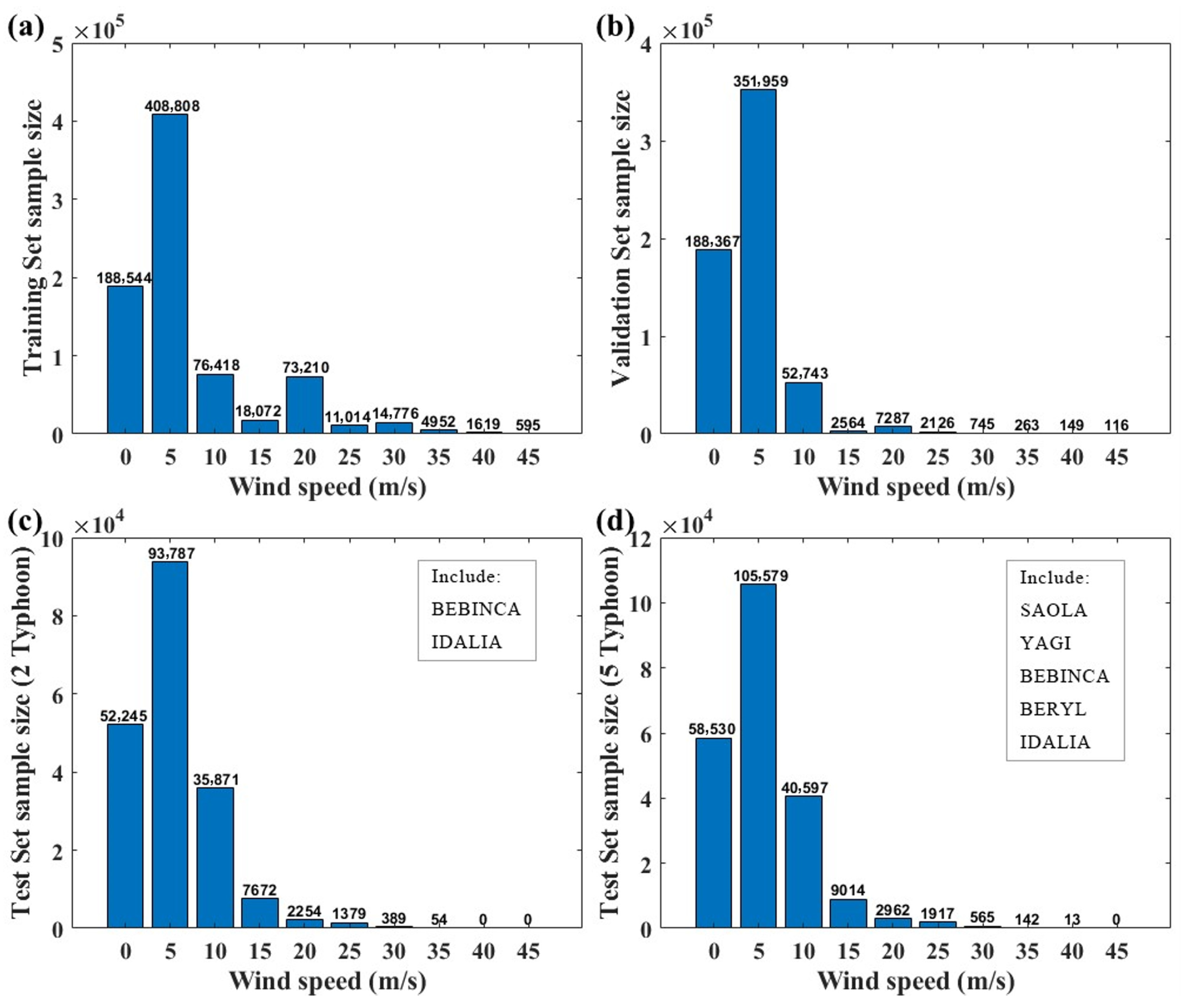
To improve representation of extreme winds in typhoon regions, this study constructed a targeted dataset. Training set augmentation included all >20 m/s samples from the entire year of 2022, all >30 m/s samples from 2019, 2020, 2021, and January–July 2023, and supplementary global 0–20 m/s samples extracted from 4 September 2022After processing, the training set contained 798,008 records (Table 1).
The validation set uses a strict out-of-time configuration: it was not sampled from the training period but instead used data from different dates: all >20 m/s samples from October 2023 together with the 0–20 m/s samples from 11 October 2023, totaling 606,319 records (Table 2). This arrangement was intended to test out-of-time generalization.
The test set comprised five representative typhoons. For each typhoon, we extracted core observation periods covering its full lifecycle from rapid intensification through peak to gradual weakening (continuous 72 h periods): Pacific—SAOLA (22 August–2 September 2023), YAGI (1–7 September 2024), BEBINCA (10–16 September 2024); Atlantic—BERYL (26 June–11 July 2024), IDALIA (26 August–8 September 2023). This ensured the test set captured the dynamic features associated with intense wind-field evolution. The selected cases differ in extreme wind speed magnitudes, geographic locations, and sample distributions. Ablation experiments primarily use the BEBINCA+IDALIA subset (193,651 records). Detailed information on the test set is provided in Table 3.
The training, validation, and test sets were strictly separated by time to prevent data leakage. Their sample-size distributions are shown in Figure 2 (5 m/s intervals; vertical axis: sample count).

3.3. Feature Selection

The CYGNSS Level 1 (L1) data product contains numerous satellite observables, such as the NBRCS and Leading-Edge Slope (LES), both of which are influenced by wind speed and sea surface roughness [32,33]. Research has shown that the two-dimensional delay–Doppler power waveform of GNSS-R signals is highly sensitive to wind speed variations, which can introduce significant errors in wind speed retrieval [26,34]. To reduce these errors, the model incorporates multi-dimensional features—encompassing signal energy, delay, and full DDM characteristics—to better capture their relationship with wind speed. Accordingly, 26 wind speed-relevant features were derived from the CYGNSS L1 data to improve model performance [10,32,35]. These encompass energy-related parameters (e.g., NBRCS, DDM peak Doppler column, LES, and DDM SNR); delay-related parameters (e.g., DDM peak delay row, specular point delay correction, and flight-software-derived specular point delay); and DDM geometry parameters (e.g., CYGNSS/GPS positions, velocities, and incidence angles) [36].
For wind speeds exceeding 20 m/s, relying solely on CYGNSS parameters proved insufficient for improving retrieval accuracy [19]. To resolve this, four environmental parameters—Mean Sea Level Pressure (MSL), Sea Surface Temperature (SST), Total Precipitation (TP), and Significant Wave Height (SWH)—were incorporated. A parameter sensitivity experiment using the validation set demonstrated their impact on the CLCTG model’s performance. When using only the 26 CYGNSS parameters, the RMSE for Typhoon YAGI in the >20 m/s range was 7.88 m/s. After adding the environmental parameters, the RMSE decreased to 5.45 m/s, confirming their critical role in high-wind-speed scenarios.
In total, 30 parameters—26 CYGNSS-derived and 4 environmental—were selected for the model, as detailed in Table 4. By integrating these parameters, the model better captures real-world conditions, significantly enhancing prediction performance.

3.4. Construction of CLCTG Model

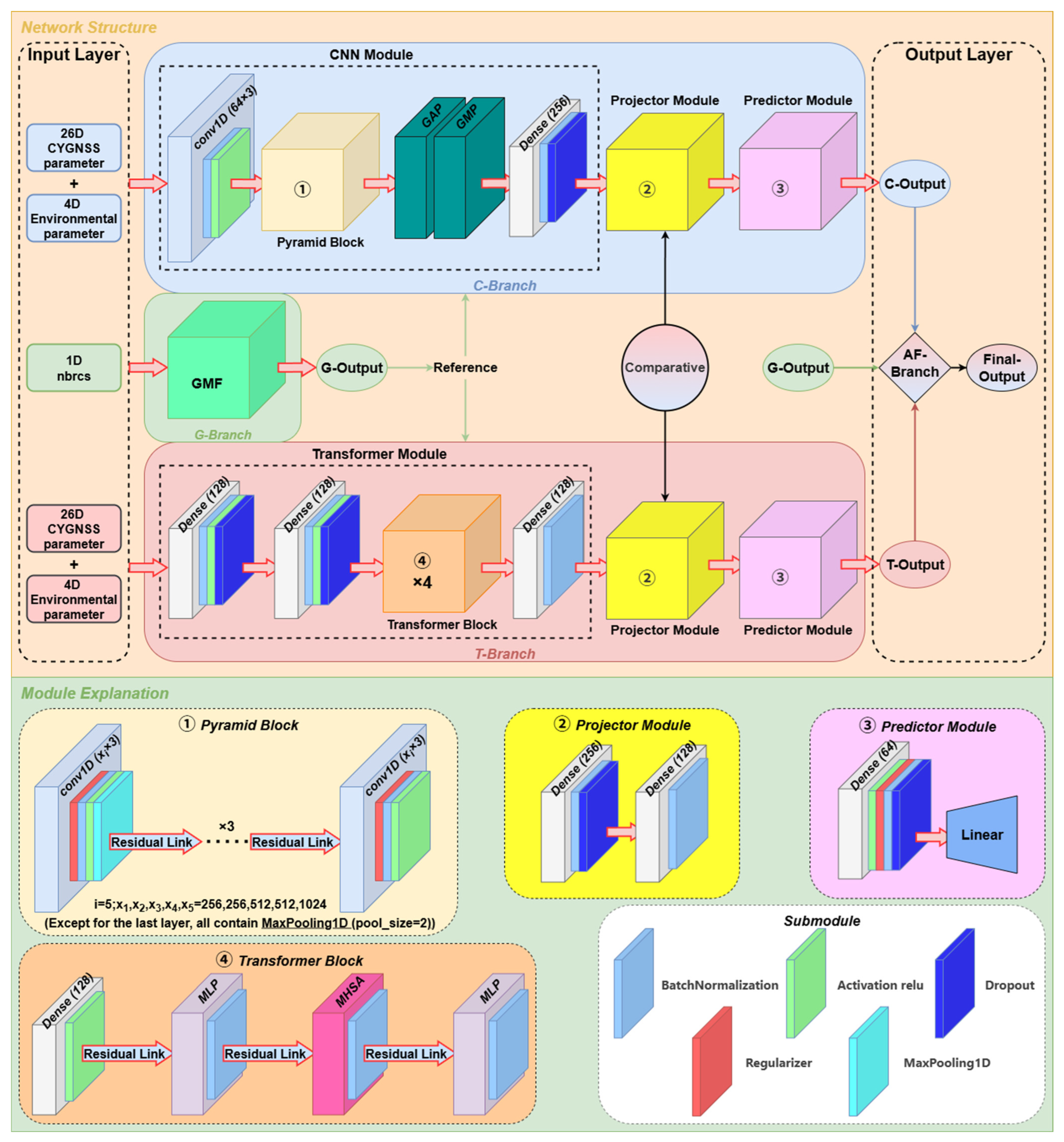
The CLCTG model consists of four key components: a CNN branch (C-Branch), a Transformer branch (T-Branch), a GMF branch (G-Branch), and an adaptive fusion branch (AF-Branch); the architecture is shown in Figure 3. Each sample corresponded to a single L1 GNSS specular reflection (one PRN at a specific time). The input was a 30-dimensional feature vector (26 CYGNSS parameters + 4 environmental variables), which was standardized by a StandardScaler and then reshaped to (30, 1).
C-Branch: input (30, 1). This begins with an initial 1D convolution (64 filters, kernel = 3), followed by a five-layer pyramid module (1D convolution filters = [256, 256, 512, 512, 1024]. All layers except for the last layer are followed by MaxPooling1D). The pyramid multi-scale outputs are pooled by Global Average Pooling (GAP) and Global Max Pooling (GMP), concatenated, passed through a fully connected layer, and then routed to a projection head and a prediction head.
T-Branch: The input is first mapped by two fully connected layers (Dense) to shape (30, 128), then passed through four Transformer blocks (the number of multi-head attention heads in the i-th layer = 4 × (i + 1); each block is followed by an MLP (256) plus residual connections and normalization). Dropout is increased progressively across layers to capture second-order and higher-order nonlinear interactions. The final output is passed through a fully connected layer and then to a projection head and a prediction head.
G-Branch: This computes GMF wind speed from the single-parameter NBRCS:
u = A e B σ 0 + C e D σ 0
The parameters fitted on the training set are A = 43.2987, B = −0.1420, C = 2.8226, and D = −0.0009 (parameters obtained from the training data). The G-Branch serves both as a physical prior guide for the C/T branches in the low- to moderate-wind-speed range and as a weighted component within the AF-Branch. Through the fusion mechanism and regression loss, it partially corrects its systematic bias, as the GMF exhibits relatively good statistical stability across different times and environments [37,38].
During training, the C-Branch and T-Branch are optimized not only by their individual regression objectives but also jointly in the projection space via contrastive learning. Contrastive learning treats the projection of the same sample from the C/T branches within a batch as a positive pair and projections of different samples as negative pairs; however, instead of the conventional hard positive/negative partitioning, we employed a soft-label matrix T to encode prior similarities between samples. The diagonal elements T i i = 1 (treating the same sample as a strong positive). If the true wind speed difference between two samples in the batch is 0.1 m/s, a small weight (e.g., 0.05) is assigned to the corresponding off-diagonal entries T i j and T j i . Each row is then normalized to sum to 1; all other elements are set to 0. This scheme treats identical samples as the primary positive examples while allowing closely valued wind speed samples to retain part of a positive association, thereby smoothing the effect of sample continuity.
The similarity matrix S is computed from the projection vectors of the two branches as follows: Projection vectors are L2-normalized, their dot products are computed and scaled by the temperature parameter τ , and a softmax is applied to produce, for each sample, a similarity distribution with respect to other samples in the batch. For loss, because our task is regression over continuous wind speed, we used the KL divergence to align the model output distribution S i with the preset soft label T i , rather than using InfoNCE, which strictly partitions samples into hard positives and negatives. This design enables the soft-label matrix to capture continuous similarities among samples (e.g., samples with proximal wind speeds should have higher affinity), making the approach more naturally suited to regression tasks where feature evolution is continuous.
The relevant loss function in the model is defined as follows:
L K L = 1 N i = 1 N K L T i S i
where N is the batch size, T i and S i are the i -th row vectors of the soft label matrix and similarity matrix, respectively, and K L · · quantifies the difference between two probability distributions. For each sample i ,
L K L i = j T i j log T i j S i j
where   T i j and S i j are elements of the soft-label matrix and the softmax-normalized similarity matrix, ensuring they conform to probability distributions.
This loss pulls together identical samples (and samples with very similar wind speeds) in the C/T projection space while pushing apart samples with large wind speed differences, thereby enhancing the discriminability of the projection representations and the sensitivity to small wind speed differences; this helps reduce single-branch bias and improve generalization.
After forward inference, the individual predictions from the three branches (C, T, and G) are fed into the adaptive fusion branch to produce the final wind speed estimate. This branch adopts an uncertainty-aware fusion strategy, whose core principle is to assess the confidence of each prediction source by quantifying local statistical variability, thereby enabling adaptive weight adjustment: “higher variability corresponds to lower weight, while greater stability corresponds to higher weight.” This strategy effectively balances the physical-reference advantage of the GMF in the low-wind-speed regime with the data-representation capability of deep learning in the high-wind-speed regime, providing clear physical interpretability for the fusion process and consequently improving overall prediction accuracy.
The specific procedure is as follows. For each branch’s prediction sequence x i ( i = C , T , G ), compute local statistics over a sliding window: the local mean μ i , local standard deviation σ i , and local coefficient of variation C V i :
μ i = A v e r a g e P o o l i n g x
σ i = A v e r a g e P o o l i n g ( ( x i μ i ) 2 )
C V i = σ i μ i + ϵ
where ϵ is a small constant to avoid division by zero.
After computing the local statistical properties, the reliability weights w i ( i = C , T ) for the C-Branch and T-Branch are computed as
w i = 1 C V i + ϵ × 1 σ i + ϵ
w i = w i w i
Since the G-Branch’s results are only partially integrated, its reliability weight is computed separately. To ensure a smooth transition between fused and non-fused intervals, a smoothing function is introduced to gradually adjust the G-Branch’s weight w G with wind speed v :
w G b a s e = c l i p v t h v 5 + 1 , 0 , 0.3
w G = w G b a s e × 1 σ G + ϵ
where v t h is the wind speed threshold at which the G-Branch participates in fusion (15 m/s). The fusion threshold is set to 15 m/s instead of the 20 m/s used during training because experimental results in Section 4.1 demonstrate that GMF output accuracy significantly degrades when wind speeds exceed 15 m/s.
The final prediction x F is a weighted sum of the C-Branch, T-Branch, and G-Branch outputs:
L K L i = j T i j log T i j S i j
where w C and w T denote the weights for the C-Branch and T-Branch outputs, and w G denotes the weight for the G-Branch output. The AF-Branch dynamically adjusts these weights at prediction time; its output is not included in the training loss and is used solely for inference-time fusion.
The specific experimental configuration is shown in Table 5.

3.5. SHAP Value Analysis

SHAP (SHapley Additive exPlanations) [39] is a highly flexible framework applicable to any machine learning model. Inspired by LIME (Local Interpretable Model-agnostic Explanations) [32] and Shapley values [40], it explains model behavior by estimating the marginal contribution of each input feature to the model’s expected prediction. It should be made clear that SHAP describes how the model internally uses input features to form predictions, not direct proof of causal relationships between features and true physical processes; therefore, the following interpretations are intended to clarify the consistency or inconsistency between model behavior and physical expectations, rather than to substitute for independent physical validation. This experiment computed SHAP values using the Kernel SHAP method based on shap.KernelExplainer, which is suitable for hybrid model architectures and approximates Shapley values through weighted linear regression.
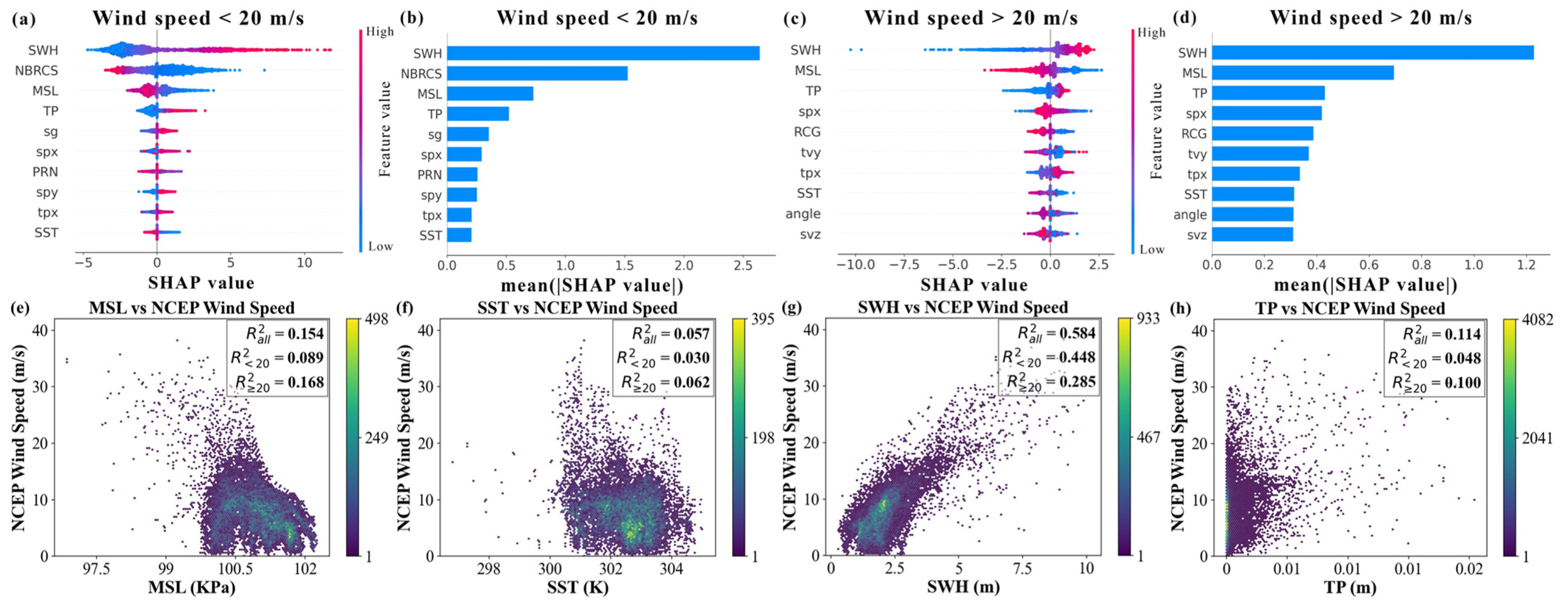
This analysis is based on the two typhoons with the largest sample counts in the test set—BEBINCA and IDALIA—from the Eastern and Western Hemispheres, totaling 193,651 samples (see Figure 2c). For segment-wise comparison, wind speed was divided into eight intervals (0–5, 5–10, 10–15, 15–20, 20–25, 25–30, 30–35, >35 m/s), and 500 samples were randomly drawn from each interval. Specifically, Figure 4a,b present the results of 2000 samples from the first four intervals (0–20 m/s); Figure 4c,d present the results of 2000 samples from the latter four intervals (20→35 m/s); the environmental-parameter vs. wind speed correlation plots in Figure 4e–h were drawn using the entire test set of 193,651 samples; the SHAP waterfall plots in Figure 5 and the SHAP-contribution correlation heatmaps in Figure 6 present the results of a total of 4000 samples covering all eight intervals.
Figure 4 presents feature importance analysis and environmental feature correlations for the CLCTG model. Figure 4a,c show SHAP summary plots for wind speeds < 20 m/s and >20 m/s, respectively. Each point represents a feature’s SHAP value for one sample: the x-axis indicates the SHAP value magnitude (direction and degree of contribution to model output), the y-axis lists feature names, and the color bar represents raw feature values (red: high, blue: low). Figure 4b,d list the top ten features by mean absolute SHAP value in each wind speed segment. In Figure 4a,b (<20 m/s), SWH, NBRCS, and MSL show relatively high mean absolute SHAP values. Within the model, high/low values of SWH typically correspond to upward/downward adjustments of the prediction, while low MSL tends to increase model output—behavior that is consistent with the physical expectation that “increasing wind speed accompanies decreasing pressure.” This “consistency” should be understood as the model’s manner of using these variables to make judgments, not as proof of physical causality. Analysis of Figure 4c,d (>20 m/s) shows that SWH and MSL remain important, and CYGNSS features (such as spx and RCG) also rise in rank, indicating that the model relies on a combination of environmental background and satellite-observation features in the high-wind regime.
Figure 4e–h show scatter plots and linear fit R 2 values between four environmental parameters (MSL, SST, SWH, TP) and NCEP wind speeds across the entire test set (193,651 samples)—for full-range, <20 m/s, and >20 m/s partitions. Results indicate all parameters correlate with wind speed at varying intensities and trends: MSL: R 2 = 0.154 (full), 0.089 (<20 m/s), and 0.168 (>20 m/s), showing a negative correlation that is strongest at high winds; SWH: R 2 = 0.584 (full), 0.448 (<20 m/s), and 0.285 (>20 m/s), showing the strongest positive correlation but weakening at high winds; TP: R 2 0.114 (full), 0.048 (<20 m/s), and 0.100 (>20 m/s), ranking second after SWH and MSL; SST: R 2 = 0.057 (full), 0.030 (<20 m/s), and 0.062 (>20 m/s), showing the weakest correlation. Although these features exhibit weak correlations in the >20 m/s range, as auxiliary physical background information they can provide the model with additional constraints and help reduce prediction uncertainty in the high-wind-speed regime. However, these features sometimes exhibit low R 2 (for example <0.2) and weak linear correlations; therefore, such statistical associations should be regarded as characterizations of information available to the model rather than as physical validation.
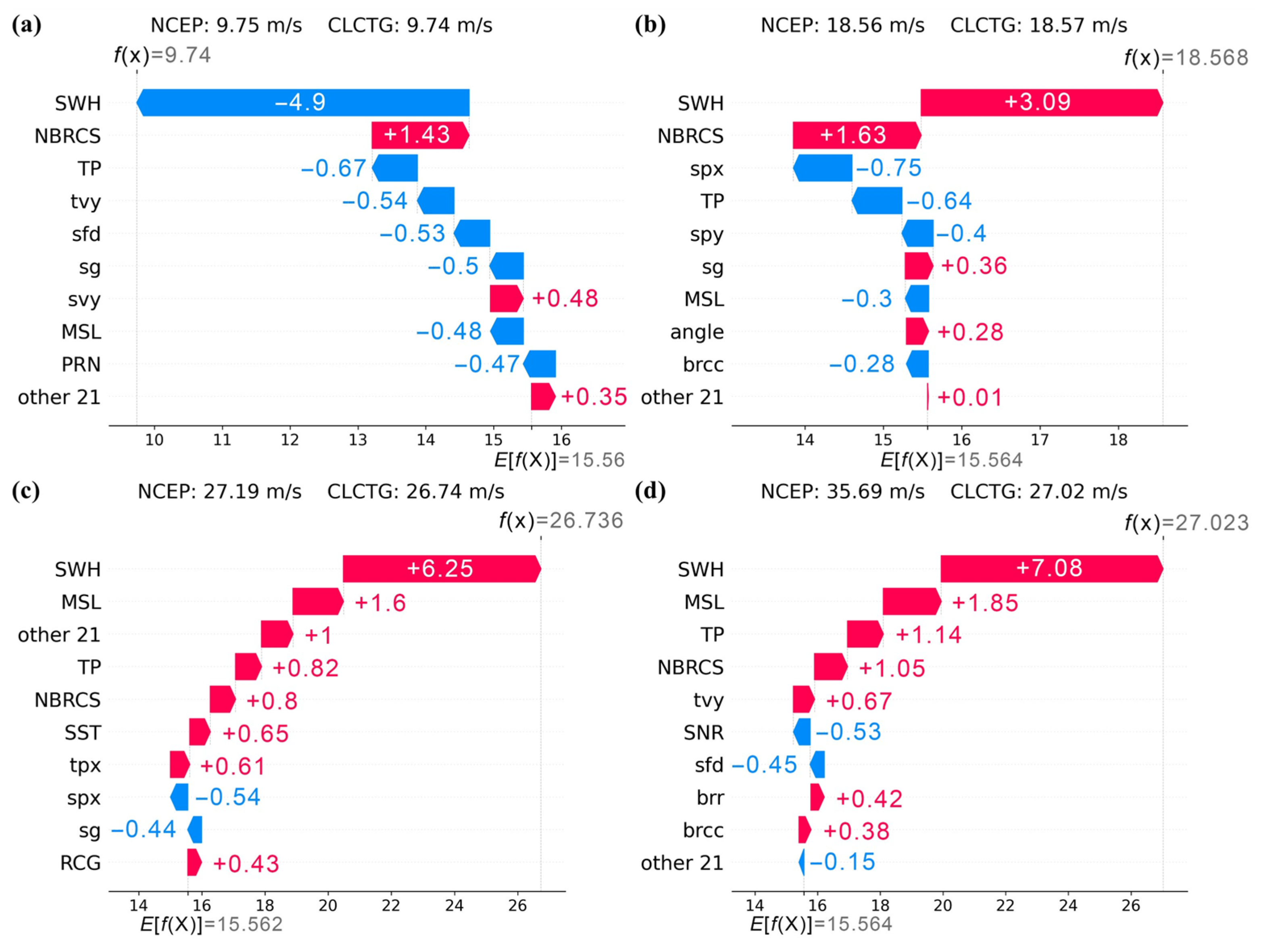
To probe the contribution mechanisms of features across wind speed ranges, Figure 5 presents SHAP waterfall plots for the CLCTG model. In the waterfall plots, E[f(x)] is the baseline equal to the mean prediction over all samples; each horizontal bar represents a single feature’s contribution to that sample’s prediction (length = |SHAP value|), with red bars indicating positive contributions and blue bars indicating negative contributions. These contributions accumulate from E[f(x)] to yield the actual prediction f(x). In the low-wind example (9.75 m/s, Figure 5a) and the moderate-wind example (18.56 m/s, Figure 5b), the positive and negative feature contributions jointly adjust the baseline to values close to the reference (CLCTG = 9.74 m/s vs. NCEP = 9.75 m/s, and CLCTG = 18.57 m/s vs. NCEP = 18.56 m/s). In the 27.19 m/s example (Figure 5c), environmental parameters provide a substantial positive push which, together with CYGNSS features such as NBRCS, brings the prediction (26.74 m/s) close to the reference wind speed. For the very high-wind example of 35.69 m/s (>30 m/s) (Figure 5d), although several environmental and CYGNSS features give positive contributions within the model, the accumulated contributions are insufficient to bridge the gap with the observations and training labels. This results in an error of approximately 8.67 m/s, reflecting the retrieval bottleneck in the >30 m/s range. The waterfall plots illustrate the model’s decision mechanism and the direction of feature effects: environmental parameters play important roles across wind speed ranges, while CYGNSS features such as NBRCS serve an auxiliary regulatory function.
In summary, we regard SHAP analysis as an important tool for evaluating and understanding the model’s internal decision logic: it helps identify which variables the model treats as key signals and the relative roles of those variables across different wind speed intervals.

3.6. Evaluation Metrics

The performance of the CLCTG model was quantitatively assessed using RMSE and Mean Absolute Error (MAE). RMSE is defined as the standard deviation (STD) of residuals between retrieved and reference wind speeds, as shown in Equation (14):
R M S E = 1 N j = 1 N u ^ j u j 2
MAE measures the average absolute difference between retrieved and reference wind speeds, as given in Equation (15):
M A E = 1 N j = 1 N u ^ j u j
The Coefficient of Determination (R2), as shown in Equation (16):
R 2 = 1 i = 1 n y i y i ^ 2 i = 1 n y i y i ¯ 2
Additionally, to evaluate the distribution consistency between CLCTG-retrieved wind speeds and other reference wind speeds, the Kolmogorov–Smirnov test (KS test) was introduced. The KS statistic quantifies the distance between two sample distributions by measuring the maximum absolute difference of their empirical cumulative distribution functions (ECDFs):
D = s u p x F C L C T G x F r e f x
where F C L C T G x and F r e f x represent the ECDFs of CLCTG retrieval results and reference wind speeds, respectively, and s u p x denotes the supremum over all x . A smaller KS value indicates greater similarity in the distributions of the two wind speed sample groups.

4. Results and Discussion

In this section, we present a systematic evaluation of CLCTG. Testing first employed a two-typhoon test set with a total of 193,651 samples (Figure 2c) to analyze the effectiveness of the three-branch fusion and to compare performance against several baseline models in typhoon scenarios. Feature ablation experiments were also used to quantify the contribution of different feature groups to predictive accuracy. To evaluate performance across wind speed ranges, the ground truth was divided into five segments with 5 m/s intervals (0–5, 5–10, 10–15, 15–20, >20 m/s) and analyzed segment by segment. The model’s cross-typhoon generalization was then tested using an independent set of three Eastern-Hemisphere and two Western-Hemisphere typhoons, with performance assessed separately for the 0–20 m/s and >20 m/s ranges. Finally, all retrieval results were validated against NCEP reanalysis, CYL2, IBTrACS typhoon data, and NDBC buoy observations; reported values are the mean of three independent retrieval runs to ensure result robustness.

4.1. Branch Ablation Experiments

The final output of the CLCTG model integrates predictions from the C-Branch, T-Branch, and G-Branch through the AF-Branch. The AF-Branch employs a dynamic weighting strategy, adaptively assigning fusion weights to the three outputs based on local statistical characteristics across wind speed intervals. To evaluate the effectiveness of this strategy, six ablation experiments (AB-S1 to AB-S6) were designed and compared with the full CLCTG:
  • AB-S1/2/3: The C/T/G branches trained jointly, outputting only C, T, or G branch results respectively;
  • AB-S4/5: The G-Branch was removed, and only the C/T branches trained, outputting only C or T branch results;
  • AB-S6: The G-Branch was removed, and only the C/T branches trained, with both outputs fused by the AF-Branch;
  • CLCTG: All three branches trained jointly, with all outputs fused by the AF-Branch.
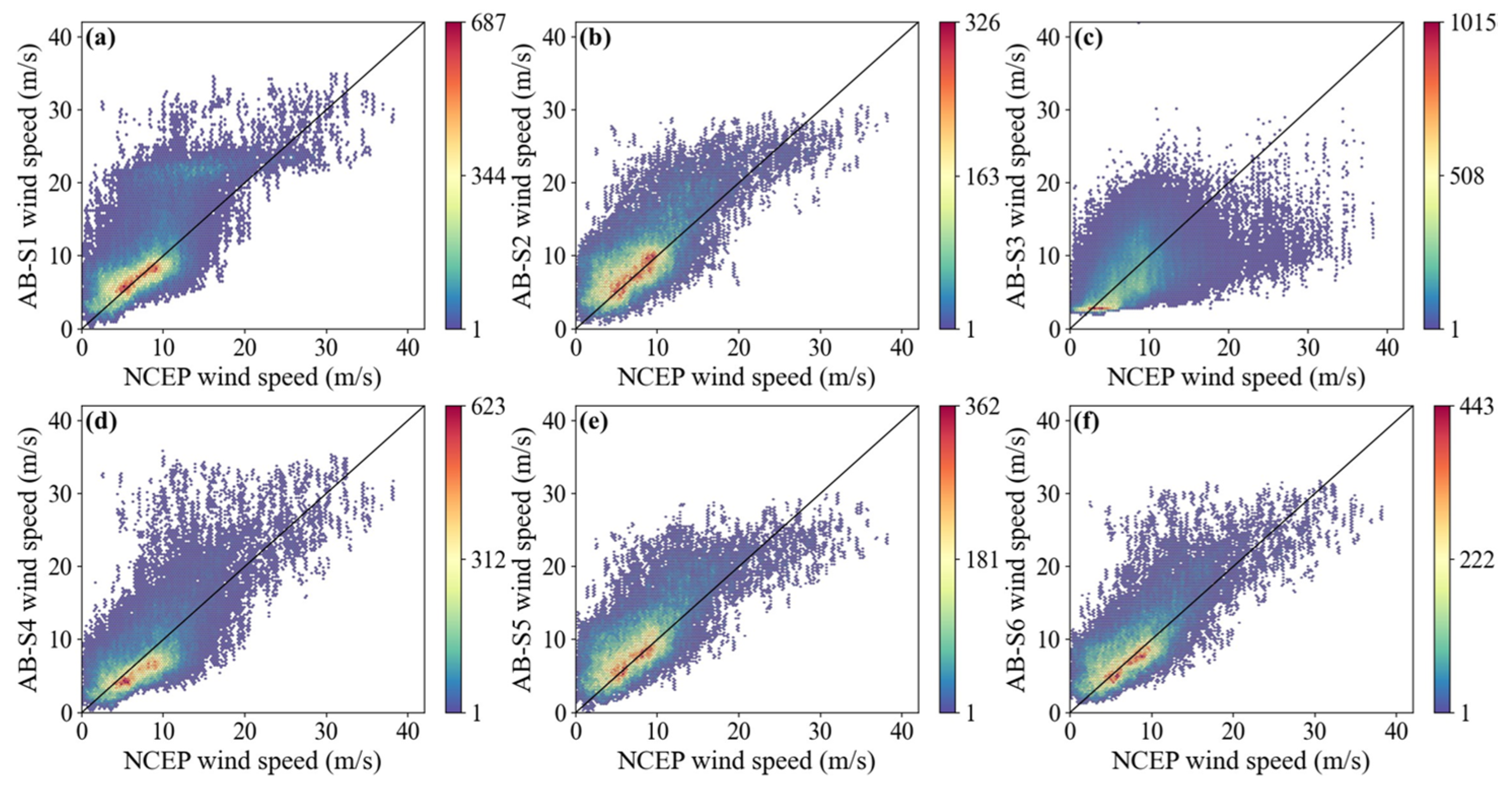
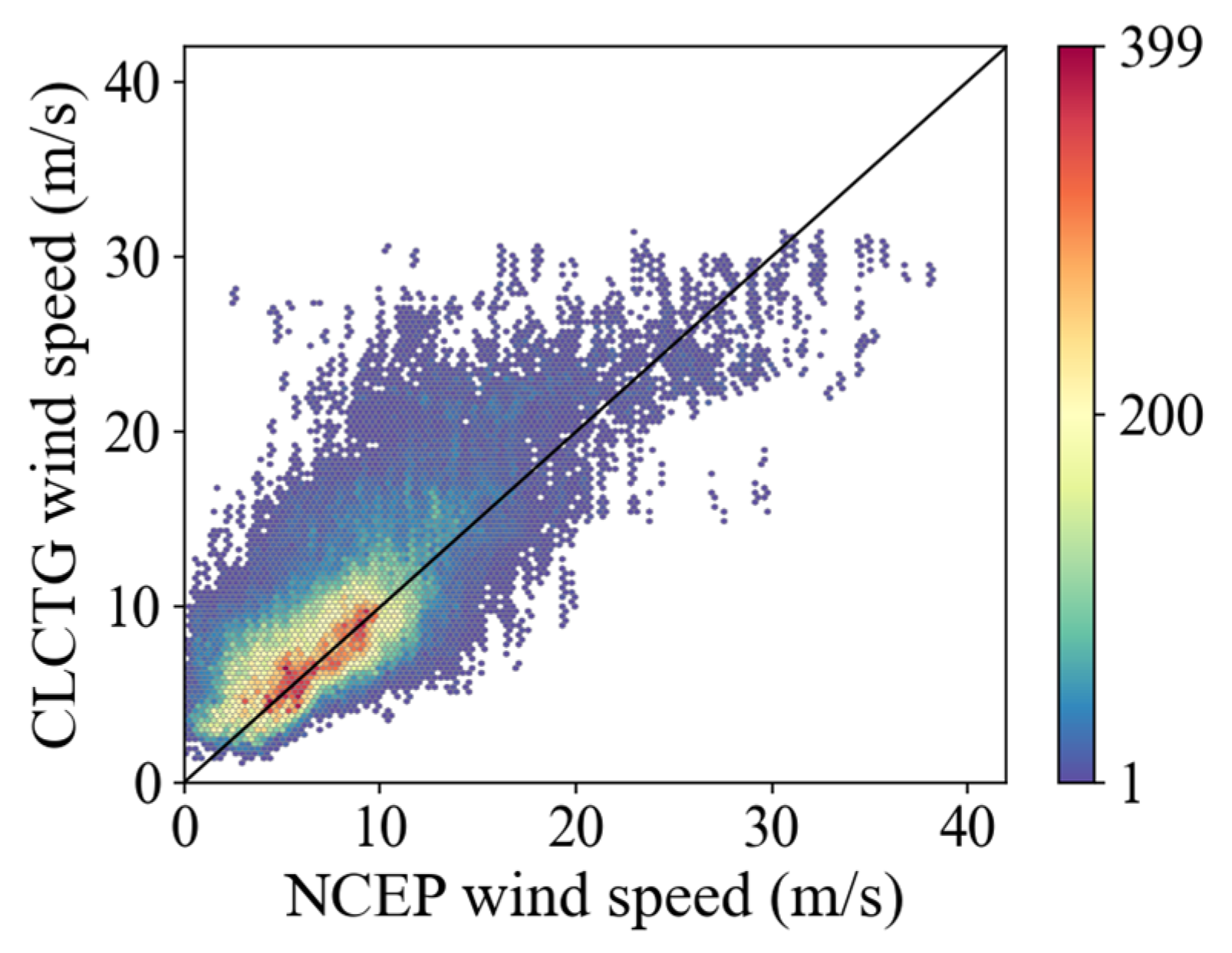
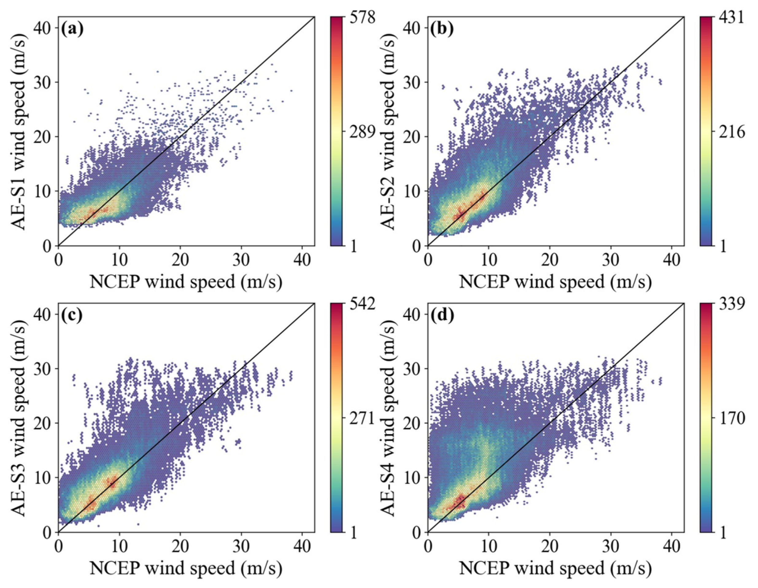
Figure 6 and Figure 7 compare density scatter plots against reference wind speeds (NCEP) for each experimental configuration and CLCTG, while Table 6 quantifies RMSE performance across wind speed intervals.
Analysis of AB-S1, AB-S2, AB-S3, and CLCTG reveals distinct advantages of single branches in specific wind speed ranges. AB-S1 shows significant errors in <20 m/s intervals, especially at 15–20 m/s (RMSE = 5.53 m/s, Figure 6a); AB-S2 is relatively balanced (all RMSE = 3.48 m/s) but slightly underestimates >20 m/s (Figure 6b); AB-S3 performs best at 0–5 m/s (RMSE = 2.96 m/s, Figure 6c) but then deteriorates rapidly for >15 m/s, reaching an RMSE of 13.76 m/s in the >20 m/s interval. This demonstrates that no single branch achieves optimal full-range retrieval.
Comparing AB-S1 and AB-S4: Removing the G-Branch priors reduces AB-S4 error at 0–5 m/s (RMSE = 2.72 m/s vs. AB-S1′s 3.75 m/s) but increases it >20 m/s (RMSE = 4.37 m/s vs. 3.78 m/s). Figure 6a,d show AB-S4 is more uniformly distributed but overall lower, while AB-S1 is concentrated at high winds. This confirms that the G-Branch priors enhance C-Branch sensitivity > 20 m/s but sacrifice 0–20 m/s accuracy.
Comparing AB-S2 and AB-S5: Similarly, AB-S5 (T-Branch without G) has lower error at 15–20 m/s (RMSE = 3.56 m/s vs. AB-S2′s 4.22 m/s) but higher >20 m/s (RMSE = 4.15 m/s vs. 3.80 m/s). Figure 6b,e show similar distributions, but AB-S2 aligns closer to the diagonal at high winds. This demonstrates that G-Branch priors improve T-Branch accuracy >20 m/s without compromising low-medium winds.
Comparing AB-S6 and CLCTG: The dual-branch AB-S6 (no G) achieves the lowest RMSE at 5–10 m/s (2.67 m/s) but underperforms CLCTG at 0–5 m/s (RMSE = 3.51 m/s vs. 3.40 m/s) and >20 m/s (RMSE = 4.15 m/s vs. 3.67 m/s). Figure 6f and Figure 7 show similar sample distributions, but CLCTG is more concentrated and aligned with the diagonal at high winds. This proves that removing the G-Branch harms high-wind characterization, while tri-branch fusion enables comprehensive coverage.
The ablation experiments clearly reveal the model architecture’s critical role: Single branches (AB-S1/2/3) excel only in specific intervals (e.g., G-Branch: RMSE = 2.96 m/s < 5 m/s but 13.76 m/s > 20 m/s), failing full-range needs. Removing the G-Branch (e.g., AB-S4 RMSE = 2.72 m/s at 0–5 m/s) improves some low winds but weakens high-wind performance (AB-S4 > 20 m/s RMSE = 4.37 m/s; AB-S5 > 20 m/s RMSE = 4.15 m/s). Dual-branch fusion (AB-S6) performs well at core speeds (5–20 m/s, e.g., RMSE = 2.67 m/s at 5–10 m/s) but has higher errors at extremes (<5 m/s: RMSE = 3.51 m/s; >20 m/s: RMSE = 4.15 m/s) than CLCTG (3.40 m/s and 3.67 m/s). In contrast, CLCTG (All RMSE = 3.30 m/s) achieves sustained low errors and high stability across all wind speeds (segment RMSE ≤ 4.30 m/s) via the AF-Branch’s dynamic fusion of data priors (G-Branch), multi-scale features (C/T branches), and adaptive weighting, fully validating the core value of this integrated architecture for holistic retrieval performance.

4.2. Model Comparative Experiments

To further validate the performance of CLCTG, this study designed four comparative experiments (CM-S1 to CM-S4) and compared their results with the full CLCTG model:
  • CM-S1: A standalone CNN identical in structure to the C-Branch in CLCTG (structure shown in Figure 3, C-Branch);
  • CM-S2: A standalone Transformer identical in structure to the T-Branch in CLCTG (structure shown in Figure 3, T-Branch);
  • CM-S3: A standalone GMF model with parameters identical to those of the G-Branch in CLCTG (A, B, C, D = 43.2987, −0.1420, 2.8226, −0.0009, respectively);
  • CM-S4: The CLCTG model with contrastive learning removed;
  • CLCTG: Comparative Learning method of CNN–Transformer with GMF fusion.
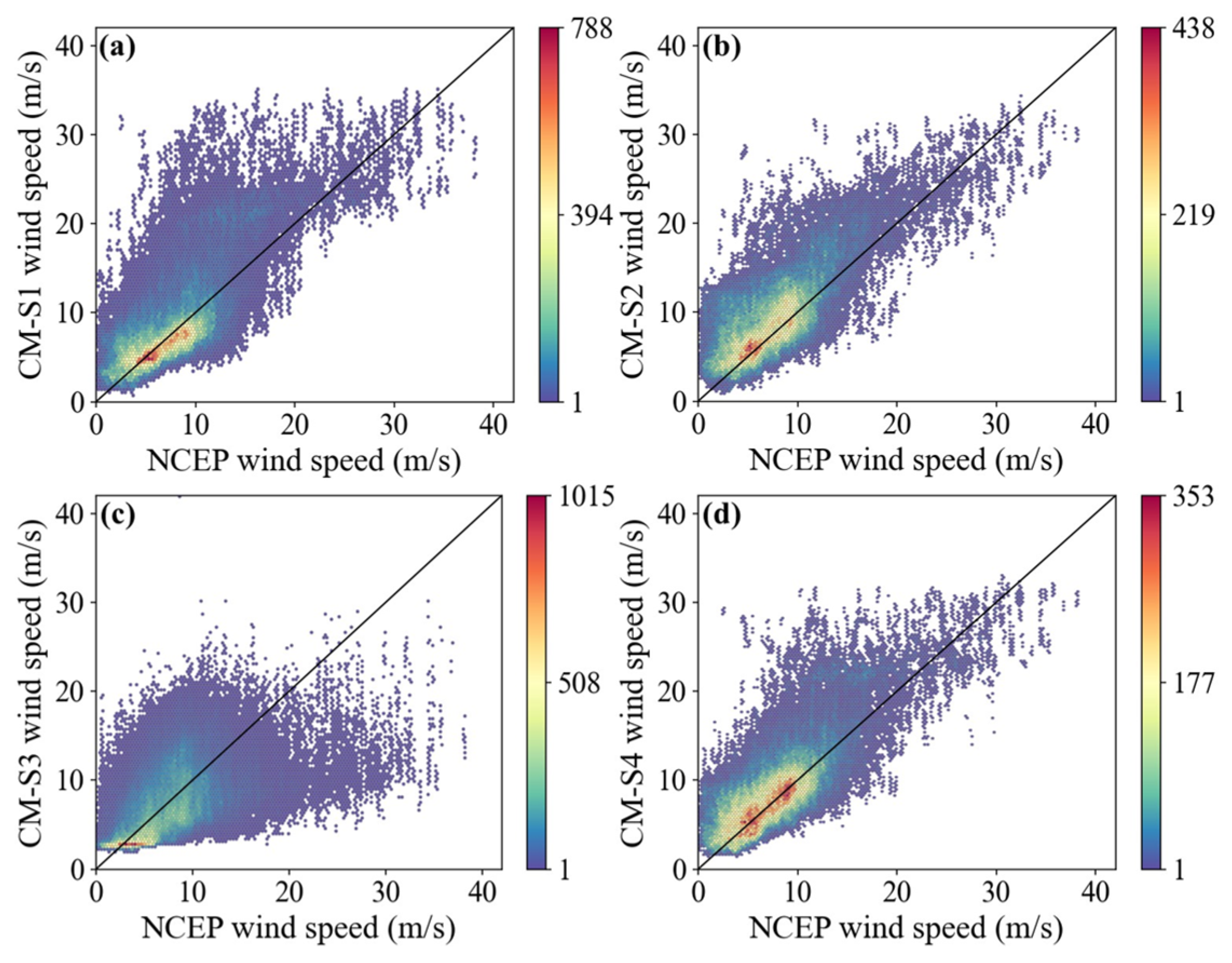
Figure 7 and Figure 8 compare density scatter plots against reference wind speeds (NCEP) for each experimental configuration and CLCTG, while Table 7 and Table 8 quantify RMSE and MAE performance across wind speed intervals.
Comparison between CM-S1 and CLCTG shows that after removing the contrastive learning mechanism, CM-S1 achieves lower error than CLCTG in the 0–5 m/s range (RMSE = 3.31 m/s vs. 3.40 m/s) but higher errors in other ranges (e.g., 15–20 m/s: RMSE = 5.54 m/s vs. 4.30 m/s). Figure 8a reveals a “stratified distribution” for CM-S1 predictions < 20 m/s (some samples underestimated, others overestimated) and dispersed predictions > 20 m/s, demonstrating that removing contrastive learning causes simultaneous over/underestimation despite minor gains at 0–5 m/s.
Comparison between CM-S2 and CLCTG indicates that without contrastive learning, CM-S2 has lower error than CLCTG at 10–20 m/s (e.g., 10–15 m/s: RMSE = 3.65 m/s vs. 3.80 m/s) but higher errors elsewhere (e.g., 0–5 m/s: RMSE = 4.39 m/s vs. 3.40 m/s). Figure 8b shows systematic overestimation < 20 m/s and scattered predictions > 20 m/s for CM-S2, confirming an overall overestimation trend after removing contrastive learning.
Compared to CLCTG, CM-S3 retains identical GMF parameters to the G-Branch in CLCTG. It indeed performs better in the 0–5 m/s range (RMSE = 2.96 m/s vs. 3.40 m/s; MAE = 2.01 m/s vs. 2.61 m/s) but exhibits significantly increased errors across all other wind speed intervals, particularly reaching RMSE = 13.76 m/s vs. 3.67 m/s and MAE = 12.94 m/s vs. 2.91 m/s for >20 m/s. Figure 8c reveals that CM-S3 samples are relatively concentrated along the diagonal within 0–15 m/s but predominantly distributed below the diagonal at high wind speeds (>20 m/s), indicating severe underestimation. This demonstrates that relying solely on the GMF physical model struggles to fully capture wind field characteristics under extreme typhoon conditions, facing a significant representation bottleneck.
The comparison between CM-S4 and CLCTG reveals that the model without contrastive learning achieves lower RMSE than CLCTG in the 0–5 m/s range (3.32 m/s vs. 3.40 m/s) and the 5–10 m/s range (2.76 m/s vs. 2.91 m/s). In the 10–15 m/s interval, its MAE is slightly below CLCTG (2.80 m/s vs. 2.81 m/s), but RMSE in this range exceeds CLCTG (3.91 m/s vs. 3.80 m/s). Furthermore, its errors are consistently higher than CLCTG for winds > 15 m/s (e.g., RMSE = 3.81 m/s vs. 3.67 m/s for >20 m/s). Figure 8d demonstrates that CM-S3 exhibits stratification in predictions within the 10–22 m/s wind speed range, with systematic overestimation for some samples and more dispersed prediction distributions above 10 m/s compared to CLCTG. This indicates that while removing the contrastive learning mechanism enhances accuracy in the 0–10 m/s interval, it induces reduced stability and accuracy for predictions exceeding 10 m/s.
Model comparison experiments showed that CM-S1 performs slightly better in the 0–5 m/s interval (RMSE = 3.31 m/s), but exhibits stratification or dispersion in the 5–20 m/s and >20 m/s ranges. CM-S2 achieves a small advantage in the 10–20 m/s band (RMSE = 3.65 m/s), yet systematically overestimates low winds (0–5 m/s RMSE = 4.39 m/s) with scattered high-wind predictions. CM-S3 excels in the 0–5 m/s segment (RMSE = 2.96 m/s vs. 3.40 m/s) but falls behind in the 5–10 m/s band (3.40 m/s vs. 2.91 m/s) and sees its error surge to 13.76 m/s for >20 m/s. CM-S4 yields relatively low errors in the 0–10 m/s range (e.g., 5–10 m/s RMSE = 2.76 m/s) but shows stratification and rising errors for winds above 10 m/s (e.g., 10–15 m/s RMSE = 3.91 m/s). Taken together, the contrastive learning mechanism—by constraining feature alignment between the CNN and Transformer branches—may introduce modest accuracy fluctuations at low to medium wind speeds but markedly boosts the model’s feature extraction capacity and prediction stability at high wind speeds (e.g., CLCTG attains only 3.67 m/s RMSE for >20 m/s). CLCTG further leverages the AF-Branch to dynamically balance physical reference against data-driven learning, while harmonizing branch outputs via contrastive learning, achieving RMSE ≤ 4.30 m/s across all wind speed intervals (>20 m/s: 3.67 m/s; overall RMSE = 3.30 m/s), thereby fully confirming the pronounced benefits of multi-branch fusion and contrastive learning for enhancing wind speed retrieval performance.

4.3. Feature Ablation Experiments

To investigate the impact of different feature combinations on CLCTG performance, feature ablation experiments with six configurations (AE-S1 to AE-S4) are compared against the full CLCTG model:
  • AE-S1: Only 4 environmental parameters (4 features);
  • AE-S2: Only 26 CYGNSS parameters (26 features);
  • AE-S3: 26 CYGNSS parameters + 3 environmental parameters (excluding MSL) (29 features);
  • AE-S4: 26 CYGNSS parameters + 3 environmental parameters (excluding SWH) (29 features);
  • CLCTG: All 26 CYGNSS parameters + 4 environmental parameters (30 features).
Figure 7 and Figure 9 compare density scatter plots against reference wind speeds (NCEP), while Table 9 and Table 10 quantify RMSE and MAE across wind speed intervals.
Comparing AE-S1, AE-S2, and CLCTG: AE-S1 achieves lower error at 5–10 m/s (RMSE = 2.10 m/s, MAE = 1.52 m/s) but significantly higher errors > 15 m/s (e.g., >20 m/s: RMSE = 4.77 m/s vs. CLCTG’s 3.67 m/s; MAE = 3.94 m/s vs. 2.91 m/s). AE-S2 (CYGNSS only) performs moderately at 15–20 m/s (RMSE = 4.18 m/s, MAE = 3.22 m/s) but suffers high errors < 15 m/s (e.g., 0–5 m/s: RMSE = 8.49 m/s, MAE = 6.14 m/s). Figure 9a shows AE-S1 overestimates at 0–5 m/s (MAE = 2.66 m/s) with scattered samples > 15 m/s; Figure 9b reveals AE-S2′s systematic overestimation < 15 m/s (e.g., 5–10 m/s MAE = 7.29 m/s) and prediction bottleneck > 15 m/s. This confirms single feature types cannot comprehensively characterize wind speeds, highlighting the complementarity of environmental and CYGNSS parameters.
Comparing AE-S3 and CLCTG: Removing MSL (AE-S3) slightly reduces errors < 15 m/s (0–5 m/s: RMSE = 3.20 m/s vs. 3.40 m/s; MAE = 2.46 m/s vs. 2.61 m/s) but increases errors > 15 m/s (e.g., 15–20 m/s: RMSE = 4.44 m/s vs. 4.30 m/s; MAE = 3.48 m/s vs. 3.46 m/s). Figure 9c reveals scattered samples >15 m/s, demonstrating MSL’s positive contribution to high-wind retrieval.
Comparing AE-S4 and CLCTG: Removing SWH (AE-S4) increases errors across all ranges (0–5 m/s: MAE = 4.19 m/s vs. 2.61 m/s; >20 m/s: MAE = 4.04 m/s vs. 2.91 m/s). Figure 9d shows simultaneous overestimation < 15 m/s (MAE = 3.83–4.19 m/s) and underestimation > 15 m/s (MAE = 3.09–4.04 m/s), confirming SWH’s indispensability for balanced characterization.
The ablation experiments revealed the following: AE-S1 excels only at 5–10 m/s (RMSE = 2.10 m/s) but degrades sharply > 15 m/s (up to 4.77 m/s). AE-S2 performs moderately at 15–20 m/s (RMSE = 4.18 m/s) but fails at 0–5 m/s (RMSE = 8.49 m/s). Excluding MSL (AE-S3) slightly benefits < 15 m/s but harms high winds. Eliminating SWH (AE-S4) introduces systematic bias (All RMSE = 5.47 m/s). In contrast, CLCTG achieves consistent accuracy (0–20 m/s RMSE ≤ 4.30 m/s; >20 m/s RMSE = 3.67 m/s; All RMSE = 3.30 m/s) through synergistic 30-dimensional feature fusion, conclusively validating the advantages in multi-source integration for typhoon wind retrieval.

4.4. Comparative Analysis of Wind Speed Retrieval for Eastern Hemisphere Typhoons (Three Cases)

To further test the generalization capability of the CLCTG model, three typhoons from the Eastern Hemisphere—SAOLA, YAGI, and BEBINCA (described in Section 3.2)—were selected. The model’s retrieval results were validated against NCEP wind speeds and CYGNSS L2 (CYL2) wind speeds.
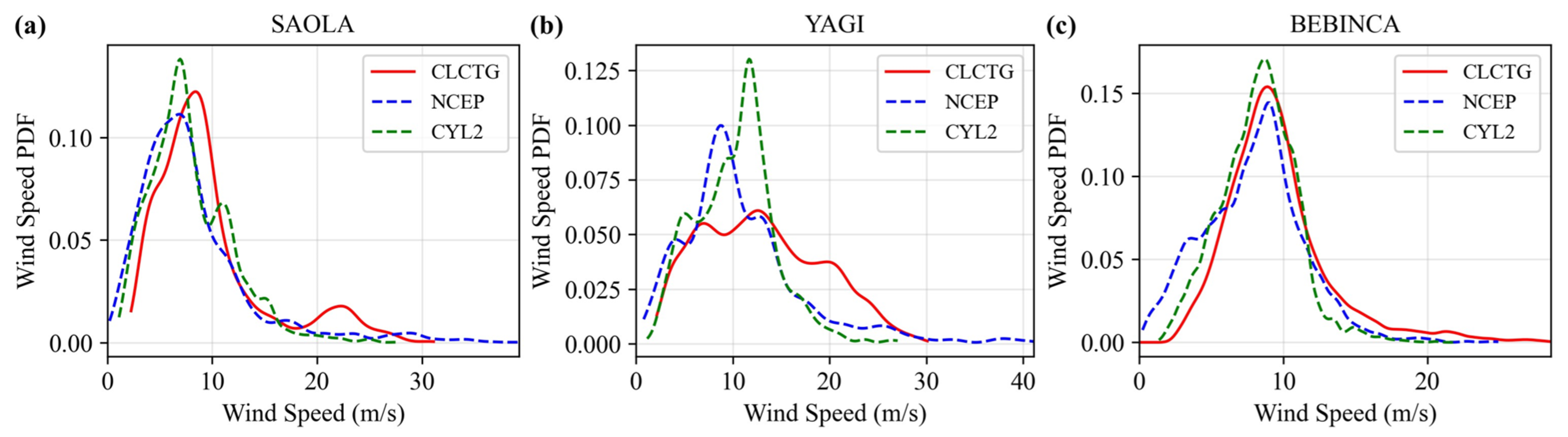
To assess reliability across wind speed intervals, probability density distributions (PDFs) and Kolmogorov–Smirnov (KS) test values between CLCTG and reference datasets (NCEP, CYL2) were compared (Table 11 and Figure 10).
In the 0–5 m/s range, CLCTG’s PDF aligns more closely with CYL2. For Typhoon BEBINCA, the KS value between CLCTG and CYL2 is 0.11, significantly lower than that with NCEP (0.35, Table 11). In Figure 10c, CLCTG’s distribution curve (blue) nearly overlaps with CYL2 (orange), indicating strong consistency. Similarly, for Typhoons SAOLA and YAGI, the CLCTG-CYL2 KS values (0.28, 0.21) are lower than the CLCTG-NCEP values (0.29, 0.24), reinforcing this trend.
In the 5–15 m/s range, CLCTG exhibits hybrid distribution characteristics. For Typhoon SAOLA, the KS difference between CLCTG-NCEP (0.13) and CLCTG-CYL2 (0.10) is minimal (0.03, Table 11). Figure 10a–c show that CLCTG’s PDF combines NCEP’s peak patterns (e.g., dense distribution near 15 m/s for SAOLA) and CYL2′s tail decay trends (e.g., smooth transition in 10–15 m/s for BEBINCA), demonstrating balanced integration of both datasets’ statistical features.
In the >15 m/s range, CLCTG aligns more closely with NCEP. For Typhoon YAGI, the CLCTG-NCEP KS value (0.12) is far lower than CLCTG-CYL2 (0.36, Table 11). In Figure 10b, CLCTG’s PDF (blue) overlaps strongly with NCEP (green) at high wind speeds, whereas CYL2 (orange) shows right-skewed deviation due to sparse extreme-speed samples. Similarly, for Typhoon BEBINCA, CLCTG-NCEP KS (0.23) outperforms CLCTG-CYL2 (0.40), confirming superior agreement with NCEP.
Taken together, across all three typhoons, composite KS values remain below 0.3 in the 0–15 m/s range (Table 11), and CLCTG’s PDF curves consistently lie between NCEP and CYL2 without significant deviation (Figure 10). For example, CLCTG’s distribution for Typhoon SAOLA closely follows both reference datasets across 0–40 m/s, while minor deviations in Typhoon BEBINCA (>30 m/s) do not disrupt overall consistency. This “dual-reference adaptability” confirms the reliability of CLCTG’s retrieval results in multi-source validation scenarios.
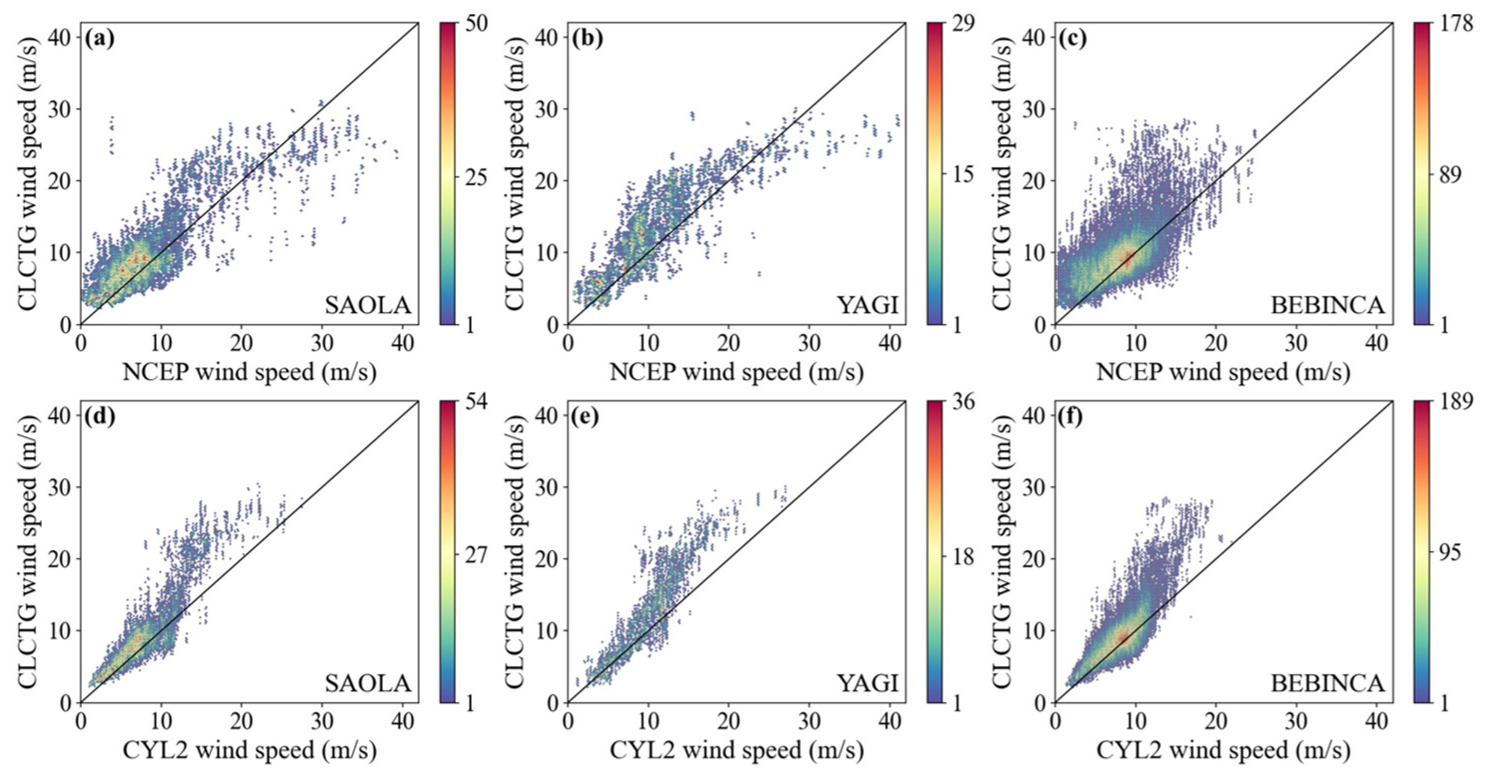
The retrieval results of the CLCTG model for three Eastern Hemisphere typhoons (SAOLA, YAGI, and BEBINCA) are compared with NCEP and CYL2 wind speeds in Figure 11 and Table 12 and Table 13.
For Typhoon SAOLA, CLCTG achieves RMSEs of 3.39 m/s (NCEP) and 3.08 m/s (CYL2), with MAEs of 2.58 m/s (NCEP) and 2.15 m/s (CYL2) (Table 12 and Table 13). As shown in Figure 11a,d, CLCTG predictions exhibit dense diagonal alignment with both reference datasets across 0–40 m/s, particularly outperforming NCEP (RMSE = 5.58 m/s) with CYL2 (RMSE = 4.38 m/s) in the >20 m/s range. For Typhoon BEBINCA, CLCTG further validates robustness at >20 m/s, achieving RMSEs of 3.39 m/s (NCEP) and 2.17 m/s (CYL2), and MAEs of 2.85 m/s (NCEP) and 2.09 m/s (CYL2) (Figure 11c,f). Typhoon YAGI shows intermediate performance (RMSE = 4.05–4.02 m/s), indicating strong adaptability to typhoon path and intensity variations (Figure 11b,e).
Within the same typhoon scenario, the CLCTG model exhibits divergent error distribution characteristics when compared to the two reference datasets. For example, in the >20 m/s range of Typhoon SAOLA, CLCTG achieves a lower MAE with CYL2 (3.74 m/s) than with NCEP (4.12 m/s), while the MAE difference in the 0–20 m/s range is smaller (CYL2 = 2.13 m/s vs. NCEP = 2.50 m/s). For Typhoon BEBINCA, CYL2 yields significantly better MAE (1.72 m/s) across all ranges compared to NCEP (2.44 m/s), whereas errors for Typhoon YAGI are nearly equivalent between references (CYL2 = 3.05 m/s vs. NCEP = 3.16 m/s). These discrepancies likely arise from differing sensitivities of data sources to wind speeds in typhoon core versus peripheral regions. Nevertheless, CLCTG maintains overall consistency with both references, as evidenced by scatter points tightly clustered along the diagonal in all subplots of Figure 11.
Across all three typhoons, CLCTG’s overall RMSE and MAE remain stable within 3.08–4.05 m/s and 1.72–3.16 m/s, respectively (Table 12 and Table 13). Density distributions in Figure 11 confirm that CLCTG predictions align closely with reference values without systematic biases, regard less of typhoon type or data source.
To summarize, the CLCTG model demonstrates robust generalization in Eastern Hemisphere typhoon scenarios, achieving consistent distribution patterns and numerical accuracy with both NCEP and CYL2 references, even under extreme wind speed conditions.

4.5. Comparative Analysis of Wind Speed Retrieval for Western Hemisphere Typhoons (Two Cases)

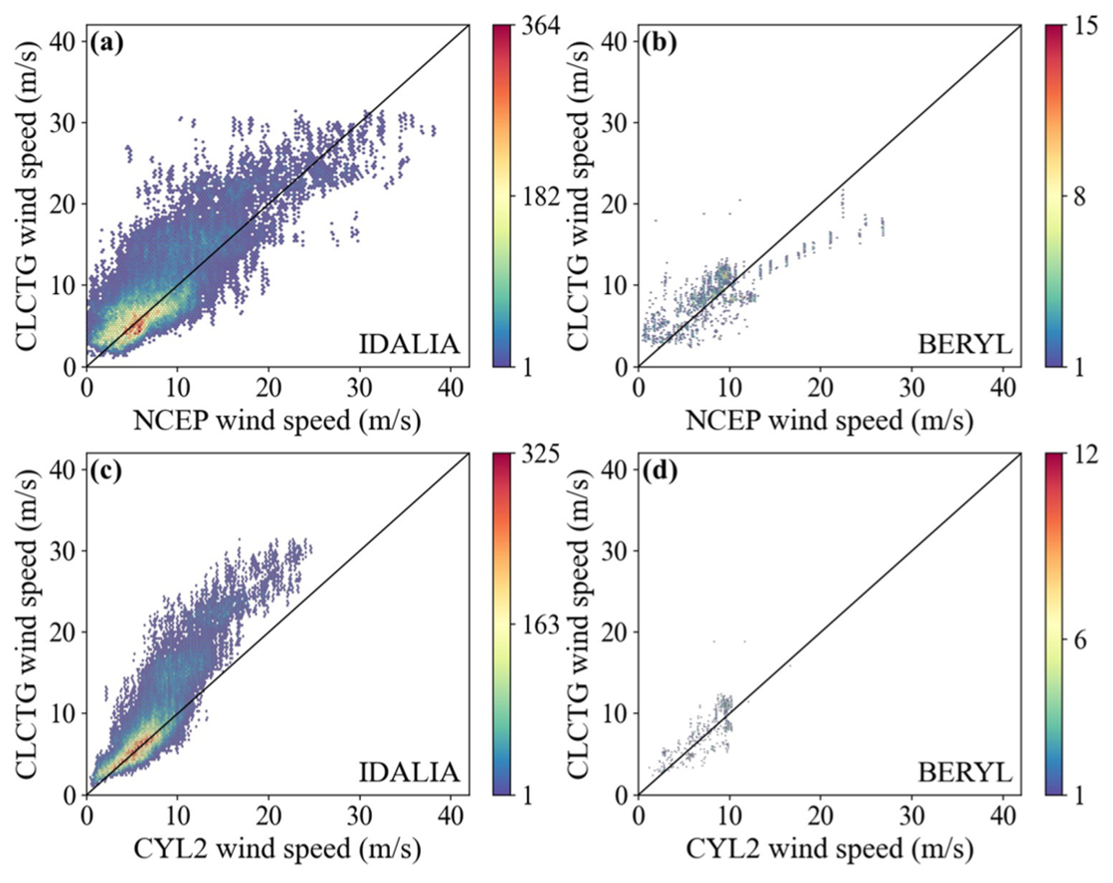
Two Western Hemisphere typhoons—IDALIA and BERYL (described in Section 3.2)—were selected. Retrieval results were validated against NCEP and CYL2 wind speeds, as shown in Figure 12 and Table 14 and Table 15.
For Typhoon IDALIA, CLCTG achieves comparable RMSE and MAE in the 0–20 m/s range (NCEP: RMSE = 3.23 m/s, MAE = 2.32 m/s; CYL2: RMSE = 3.37 m/s, MAE = 2.22 m/s). However, in the >20 m/s range, CYL2 significantly underperforms (RMSE = 6.46 m/s, MAE = 6.12 m/s) compared to NCEP (RMSE = 3.68 m/s, MAE = 2.91 m/s). Figure 12a,c show that CYL2 predictions in this range cluster above the diagonal, indicating systematic overestimation, while NCEP aligns closely with the diagonal. This discrepancy may stem from CYL2′s lower sensitivity to wind speeds in typhoon core versus periphery (NCEP wind speeds reach ~38 m/s in Figure 12a, versus CYL2′s ~31 m/s in Figure 12c). Despite this, CLCTG maintains overall RMSE (3.40 m/s) comparable to NCEP (3.25 m/s), avoiding error amplification.
For Typhoon BERYL, with limited data (total samples = 1958) and no valid CYL2 data in the >20 m/s range. In the 0–20 m/s range, CLCTG’s RMSE (1.69 m/s) and MAE (1.44 m/s) outperform NCEP (2.50 m/s, 2.02 m/s). Figure 12b,d demonstrate that both CYL2 and NCEP scatter points cluster near the diagonal, confirming CLCTG’s ability to capture observed wind speed characteristics even with sparse data. For >20 m/s, NCEP samples are scarce (sparsely distributed in Figure 12b), but CLCTG predictions remain aligned with the diagonal, reflecting adaptability to extreme wind speeds. Although direct comparison with CYL2 is unavailable, CLCTG’s stability is validated under existing data constraints.
In summary, the CLCTG model maintains consistent distribution trends with both references in Western Hemisphere typhoon scenarios, even under extreme sample scarcity (e.g., Typhoon BERYL), demonstrating robust generalization across regions with complex meteorological conditions.

4.6. Cross-Validation of Results

The CLCTG model demonstrates high reliability across different spatiotemporal regions. To further validate the reliability of its retrieval results, CLCTG’s wind speeds are compared with IBTrACS typhoon center wind speeds and NDBC buoy-measured wind speeds.
(1)
Validation with IBTrACS Typhoon Center Wind Speeds:
Comparison of CLCTG retrieval results against IBTrACS data (Table 16) reveals the model’s capability to capture wind field structures in typhoon core regions, while exposing systematic biases.
At multiple timestamps (e.g., SAOLA 29 August 2023 18:00, SAOLA 30 August 2023 18:00, and IDALIA 30 August 2023 9:00), the maximum wind speed points retrieved by CLCTG were generally higher than those at the nearest observation points (by 4–6 m/s), consistent with the physical principle that peak winds concentrate in the eyewall of a typhoon. For example, at IDALIA 30 August 2023 9:00, the nearest point (5.61 km) recorded 23.49 m/s, while the maximum wind speed point (31.65 km) reached 27.73 m/s. Conversely, in 6 out of 10 examined timestamps, NCEP’s retrievals at the maximum wind speed points were lower than or equal to those at the nearest points (e.g., BEBINCA 15 September 2024 00:00, both 5.11 m/s), failing to adequately capture the eyewall peak characteristics.
Across all examined timestamps and both reference wind speed sources, CLCTG retrievals were significantly higher than those of NCEP (average +8.2 m/s) and exceeded CYL2 in 9 out of 10 cases (average +4.1 m/s), indicating a systematic overestimation near typhoon cores. Notably, even in intense typhoon cores with reported wind speeds exceeding 59 m/s (e.g., SAOLA), CLCTG’s maximum retrievals only reached 29.87–30.45 m/s—still far below the IBTrACS center reports (59.11–71.96 m/s)—further confirming its bottleneck in representing extreme winds (>30 m/s).
CLCTG’s advantage is most pronounced in strong typhoons: At IDALIA 30 August 2023 6:00, CLCTG retrieved 25.59 m/s (nearest point) vs. NCEP’s 22.80 m/s, and 26.63 m/s (maximum point) vs. 22.80 m/s. For weak typhoons (e.g., BEBINCA), CLCTG aligns closer to CYL2 (15 September 2024 0:00: 22.72 m/s vs. 20.47 m/s at nearest point). In strong typhoons, it substantially exceeds CYL2 (e.g., SAOLA 1 September 2023 0:00: 30.45 m/s vs. 22.03 m/s at maximum point), further validating CLCTG’s superiority while highlighting extreme-wind limitations.
These findings demonstrate CLCTG’s ability to spatially resolve eyewall wind maxima, systematically outperforming NCEP in core regions. However, its overall overestimation tendency (especially in strong typhoons) and limited absolute retrieval for extreme winds (>30 m/s) are primarily attributed to training data dependency and sparse high-wind samples.
(2)
Validation with NDBC Buoy Measurements (IDALIA):
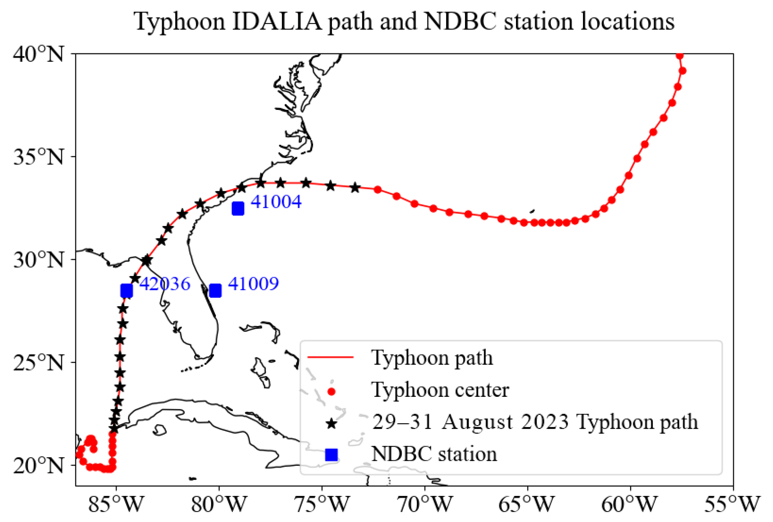
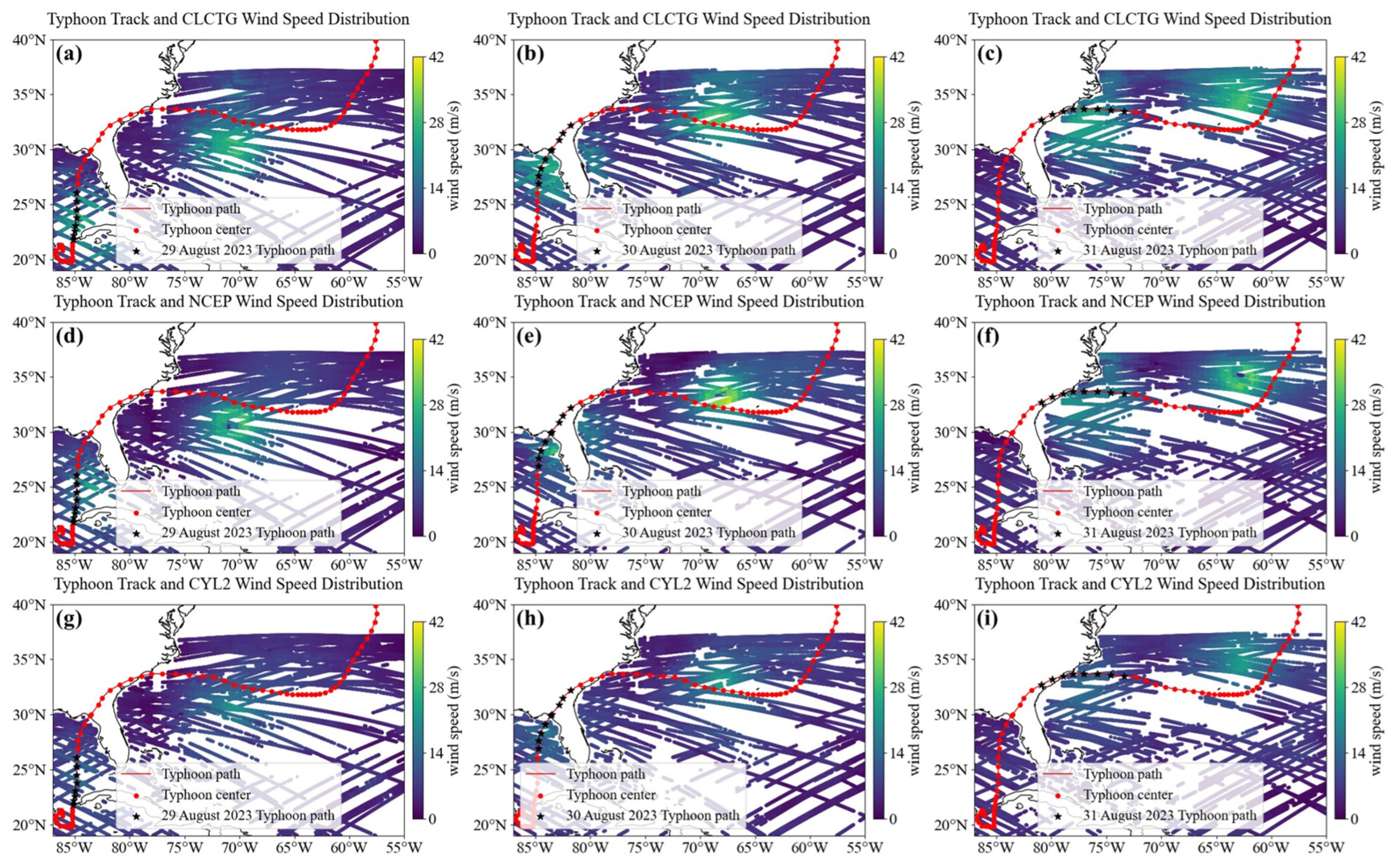
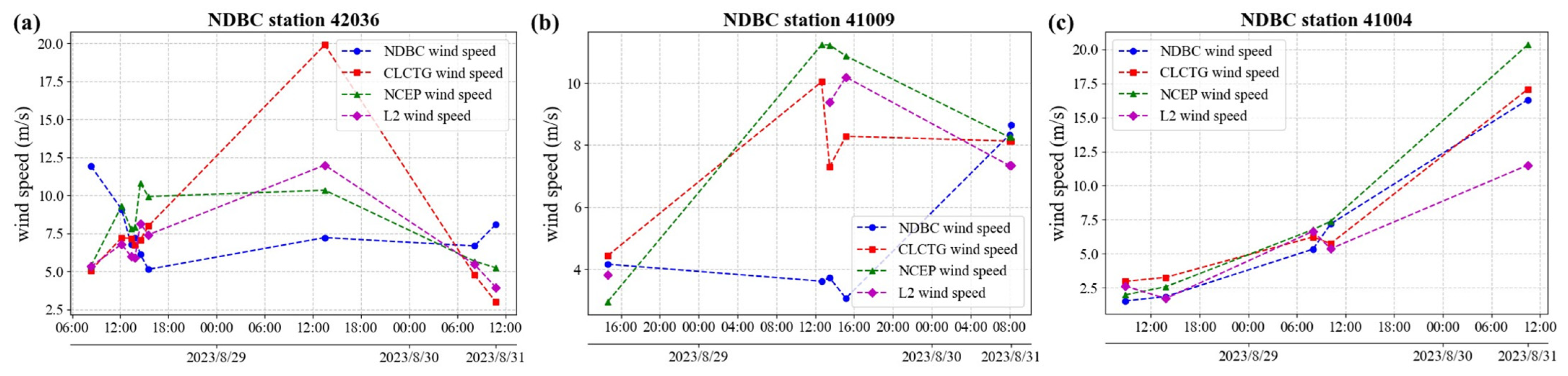
To systematically evaluate CLCTG performance across typhoon impact zones (from core strong-wind to peripheral/edge regions), three representative NDBC stations were selected: Station 42036 in IDALIA’s direct impact core, Station 41009 in the peripheral strong-wind belt, and Station 41004 in the relatively weak-wind edge region (locations shown in Figure 13). Figure 14 displays spatiotemporal wind speed maps for CLCTG, NCEP, and CYL2 during typhoon progression. Figure 15 illustrates temporal trends of model-predicted versus NDBC-observed wind speeds at these stations.
Typhoon Direct Impact Core (Station 42036, Figure 15a): This plot reveals significant systematic overestimation by CLCTG (and NCEP/CYL2) in peak-wind regions. For example, when NDBC recorded a peak of 7.4 m/s, CLCTG predicted ~19 m/s versus NCEP (10.5 m/s) and CYL2 (12 m/s). Notably, the NCEP reference wind speeds used in training (10.5 m/s) already exceeded NDBC observations (7.4 m/s), partially explaining CLCTG’s high bias versus NDBC. Post-landfall (31 August 2023), deviations decrease markedly.
Peripheral Region (Station 41009, Figure 15b): Before landfall (29 August 2023), errors in CLCTG were below 2 m/s, aligning with NCEP/CYL2 results. During typhoon passage (30 August 2023), CLCTG predictions (7.5–10 m/s) exceeded NDBC measurements (2.8–3.8 m/s) but aligned with NCEP/CYL2. Spatiotemporal maps (Figure 14b,e,h) confirm smooth wind speed gradients and structural consistency.
Edge Region (Station 41004, Figure 15c): CLCTG maintained low errors (<3 m/s) throughout, achieving near-perfect agreement at landfall (31 August 2023: 17 m/s vs. NDBC 16.5 m/s). Spatial distributions (Figure 14c,f,i) demonstrate pattern alignment with reference datasets.
Synthesizing NDBC observations (Figure 15) and the spatiotemporal evolution (Figure 14), CLCTG’s spatial distributions (e.g., gradients, relative high/low zones) show reasonable agreement with NCEP and CYL2 reanalysis products, and the CLCTG retrievals are generally closer to NDBC measurements. This confirms successful capture of typhoon wind field structures. However, numerical biases persist, including significant overestimation in cores (e.g., 42036: ~19 m/s vs. NDBC 7.4 m/s) and residual errors in peripheries.
(3)
Synthesis:
IBTrACS core validation and NDBC peripheral observations collectively indicate that CLCTG resolves spatial wind gradients (eyewall > periphery) but exhibits systematic overestimation across zones, necessitating optimized data strategies.

4.7. Discussion of Results

The CLCTG model achieves balanced retrieval accuracy across 0–30 m/s wind speeds in typhoon regions (Table 6: All RMSE = 3.30 m/s). The adaptive fusion branch effectively balances branch advantages, demonstrating strong robustness at >20 m/s (Table 6: RMSE = 3.67 m/s). SHAP analysis and feature ablation experiments (AE-S1–AE-S4) further indicate that synergistic effects among multi-source features (26 CYGNSS + 4 environmental features) enhance stability. Validation across five Eastern/Western Hemisphere typhoons and multi-source reference wind speeds (NCEP, CYL2, IBTrACS, NDBC) supports generalization capability (Figure 13 and Figure 14, Table 12, Table 13, Table 14 and Table 15). It should be emphasized that, based on the training and validation results of this study, we cautiously define the model’s applicable range as “extending the wind speed range over which GNSS-R can be reliably retrieved from approximately 20 m/s to approximately 30 m/s,” rather than claiming precise reproduction of extreme peaks exceeding 30 m/s.
However, in-depth analysis reveals some limitations:
(1)
Systematic overestimation and side effects of data augmentation: The model exhibits systematic positive bias in typhoon core regions and in the 5–15 m/s interval. For example, at IDALIA’s core (station 42036) the predicted value (~19 m/s) is substantially higher than the NDBC observation (7.4 m/s) and the NCEP value used as a training reference (~10.5 m/s) (Figure 15a). This is mainly attributable to the sample augmentation strategy adopted to increase sensitivity to high wind speeds: while it increases the “visibility” of high-wind samples, it also introduces a statistical tendency toward higher wind speeds, thereby amplifying overestimation errors in the low- to moderate-wind-speed range.
(2)
Sparsity of high-wind samples and reference-data uncertainty: Although >20 m/s samples were augmented, true >30 m/s samples still accounted for a very small fraction of the training set (~2.7%, Figure 2), resulting in insufficient learning of extreme nonlinear features and very few model outputs exceeding 30 m/s (overall proportion ≈ 0.1%). Moreover, the reference data themselves exhibit uncertainty under extreme conditions, which limits the model’s ability to retrieve the most extreme peaks. Thus, the model’s underestimation in the >30 m/s range is related both to sample scarcity and to limitations of the training labels (reference data) and observational physics.
(3)
Latency in response to dynamic wind fields: in typhoon peripheral regions (e.g., Station 41009), the model shows delayed response to abrupt wind speed changes (Figure 15b). This arises because the AF-Branch’s fusion strategy based on local statistics tends to over-smooth instantaneous fluctuations in rapidly changing scenarios.
(4)
Model complexity and parameter sensitivity: The proposed multi-branch fusion architecture introduces relative structural complexity, and its performance depends on the coordination of multiple components and empirical thresholds within the adaptive fusion. Although Section 4.2 demonstrates the need for the current architecture, the various hyperparameters embedded in the model have not yet been subjected to a systematic sensitivity analysis.
To address the above issues, future improvements will focus on (i) optimizing adaptive sample augmentation strategies by shifting from “simply amplifying high-wind samples” toward adaptive augmentation and stratified resampling based on typhoon intensity, wind speed gradients, or local sea state to reduce adverse effects on low- to moderate- wind-speed segments; (ii) expanding and multi-sourcing training references by incorporating datasets with reliable high-wind observations (e.g., SFMR, SAR, or lidar) into training/validation, or adopting multi-source weighted labeling to mitigate systematic bias from a single reference; (iii) explicitly accounting for reference data uncertainty during training and evaluation (for example, adding label-variance-based weighting terms to the loss function or adopting probabilistic/Bayesian label-uncertainty modeling) to reduce blind reliance on biased labels; (iv) enhancing the AF-Branch’s real-time responsiveness by introducing short time-window features, wind gradient descriptors, etc., to improve response to rapidly evolving wind fields; (v) designing extrapolation or correction modules targeted at extreme wind speeds to progressively mitigate underestimation in the >30 m/s range; (vi) performing systematic sensitivity analysis of key model hyperparameters and exploring model simplification pathways that preserve performance. Additionally, the current test sample of five typhoons from the Eastern and Western Hemispheres is limited, but these cases were selected to cover different hemispheres and intensity conditions; subsequent work will expand the sample set and perform targeted sensitivity/alternative-reference comparisons to quantify the specific impacts of the factors described above on performance.
In summary, the CLCTG model demonstrates clear potential for performance improvement within the 0–30 m/s range, but further research and refinement are still needed in terms of extreme wind speed inversion, response speed, and parameter robustness.

5. Conclusions

Typhoon-region high-wind-speed retrieval over the sea remains a major challenge in meteorological remote sensing. The CLCTG contrastive learning model employs multi-branch collaboration (the CNN branch captures local coupling, the Transformer branch models global dependencies, the GMF branch uses GMF as a physical reference in the low- to moderate-wind-speed range, the adaptive fusion branch implements uncertainty-aware adaptive fusion) together with a contrastive learning mechanism based on Kullback–Leibler divergence. The framework is designed to improve retrieval robustness and generalization under conditions of sample sparsity and local failure of physical models, and to extend the range of reliable GNSS-R retrieval from approximately 20 m/s to approximately 30 m/s.
On a test set containing two typhoons from the Eastern and Western Hemispheres, the CLCTG model achieves an overall RMSE of 3.30 m/s, showing clear improvements over the traditional GMF (RMSE > 7.20 m/s) and single CNN/Transformer models (RMSE > 3.54 m/s). In the high-wind-speed regime (>20 m/s), the RMSE is approximately 3.67 m/s, indicating performance gains in strong-wind areas as well. Branch-wise ablation and uncertainty analyses further confirm the contributions of each module: KL-based alignment improves consistency between the C- and T-Branches; the GMF provides a stable physical reference in the <15 m/s range; and the adaptive fusion branch’s adaptive weighting is critical for robust performance across the full wind speed spectrum. Multi-source feature fusion (CYGNSS features and environmental variables) also plays an important role in enhancing overall performance.
At the same time, this study also identifies several key limitations (Section 4.7). Future work will concentrate on designing more balanced adaptive sample augmentation strategies; integrating multi-source references and explicitly accounting for label uncertainty; enhancing dynamic modeling and fusion responsiveness; performing systematic hyperparameter-sensitivity analysis and exploring model simplification pathways; and coordinating with SAR/SFMR observations to improve extreme-wind retrieval capability. With these improvements and more comprehensive validation, it is expected that model reliability and interpretability in extreme scenarios can be improved while maintaining performance in the 0–30 m/s range.
Collectively, CLCTG contrastive learning model, as an engineering-oriented integrated solution for extreme typhoon conditions, offers a feasible pathway to improve GNSS-R retrieval performance in complex typhoon environments by jointly leveraging data-driven methods and physical references, aligning local and global representations, and adaptively fusing them under uncertainty. It also identifies key directions for subsequent research and operational improvements.

Author Contributions

Y.Z.: conceptualization, methodology, project administration, funding acquisition; Z.T.: methodology, software, writing—original draft; S.Y.: methodology, investigation, validation; Q.S.: visualization, writing—review and editing; J.L.: data curation, validation; F.G., B.P., Y.H., and Z.H.: investigation. All authors have read and agreed to the published version of the manuscript.

Funding

This work was supported by the National Natural Science Foundation of China (Grant Nos. 42271335, 42176175) and the Shanghai Science and Technology Program (Project Nos. 24TS1402700, 24DZ3100506).

Data Availability Statement

Data available in a publicly accessible repository: The original data presented in the study are openly available in [CYCNSS; ECMWF; NCEP; NDBC; IBTrACS] at [https://www.earthdata.nasa.gov/; https://cds.climate.copernicus.eu/; https://rda.ucar.edu/; https://www.ndbc.noaa.gov/; https://www.ncei.noaa.gov/] (accessed on 20 August 2025).

Acknowledgments

We sincerely appreciate the support of the following institutions and experts for this research: We thank the CYGNSS website (https://www.earthdata.nasa.gov/) for providing CYGNSS data; the European Centre for Medium-Range Weather Forecasts (ECMWF) website (https://cds.climate.copernicus.eu/) for providing environmental parameters such as MSL, SST, TP and SWH; the National Centers for Environmental Prediction (NCEP) website (https://rda.ucar.edu/) for supplying reference wind speeds; the National Data Buoy Center (NDBC) (https://www.ndbc.noaa.gov/) for offering NDBC buoy data; and the International Best Track Archive for Climate Stewardship (IBTrACS) (https://www.ncei.noaa.gov/) for providing typhoon tracks, typhoon center wind speeds, and typhoon lifecycle data.

Conflicts of Interest

The authors declare no conflict of interest.

References

  1. Jagdish Kumar, S.V.V.A.; Chakraborty, A.; Kumar, R. Validation of wind speed retrieval from RISAT-1 SAR images of the North Indian Ocean. Remote Sens. Lett. 2018, 9, 421–428. [Google Scholar] [CrossRef]
  2. Gao, Y.; Sun, J.; Zhang, J.; Guan, C. Extreme wind speeds retrieval using sentinel-1 IW mode SAR data. Remote Sens. 2021, 13, 1867. [Google Scholar] [CrossRef]
  3. Zavorotny, V.U.; Voronovich, A.G. Scattering of GPS signals from the ocean with wind remote sensing application. IEEE Trans. Geosci. Remote Sens. 2000, 38, 951–964. [Google Scholar] [CrossRef]
  4. Komjathy, A.; Zavorotny, V.U.; Axelrad, P.; Born, G.H.; Garrison, J.L. Gps signal scattering from sea surface. Remote Sens. Environ. 2000, 73, 162–174. [Google Scholar] [CrossRef]
  5. Clarizia, M.P.; Ruf, C.S.; Jales, P.; Gommenginger, C. Spaceborne GNSS-R minimum variance wind speed estimator. IEEE Trans. Geosci. Remote Sens. 2014, 52, 6829–6843. [Google Scholar] [CrossRef]
  6. Rodriguez-Alvarez, N.; Garrison, J.L. Generalized linear observables for ocean wind retrieval from calibrated GNSS-R delay–doppler maps. IEEE Trans. Geosci. Remote Sens. 2016, 54, 1142–1155. [Google Scholar] [CrossRef]
  7. Ruf, C.S.; Balasubramaniam, R. Development of the CYGNSS geophysical model function for wind speed. IEEE J. Sel. Top. Appl. Earth Obs. Remote Sens. 2019, 12, 66–77. [Google Scholar] [CrossRef]
  8. Li, Z.; Guo, F.; Chen, F.; Zhang, Z.; Zhang, X. Wind speed retrieval using GNSS-R technique with geographic partitioning. Satell. Navig. 2023, 4, 4. [Google Scholar] [CrossRef]
  9. Liu, Y.; Collett, I.; Morton, Y.J. Application of neural network to GNSS-R wind speed retrieval. IEEE Trans. Geosci. Remote Sens. 2019, 57, 9756–9766. [Google Scholar] [CrossRef]
  10. Reynolds, J.; Clarizia, M.P.; Santi, E. Wind speed estimation from CYGNSS using artificial neural networks. IEEE J. Sel. Top. Appl. Earth Obs. Remote Sens. 2020, 13, 708–716. [Google Scholar] [CrossRef]
  11. Chu, X.; He, J.; Song, H.; Qi, Y.; Sun, Y.; Bai, W.; Li, W.; Wu, Q. Multimodal deep learning for heterogeneous GNSS-R data fusion and ocean wind speed retrieval. IEEE J. Sel. Top. Appl. Earth Obs. Remote Sens. 2020, 13, 5971–5981. [Google Scholar] [CrossRef]
  12. Asgarimehr, M.; Zhelavskaya, I.; Foti, G.; Reich, S.; Wickert, J. A GNSS-R geophysical model function: Machine learning for wind speed retrievals. IEEE Geosci. Remote Sens. Lett. 2020, 17, 1333–1337. [Google Scholar] [CrossRef]
  13. Bu, J.; Yu, K.; Zuo, X.; Ni, J.; Li, Y.; Huang, W. GloWS-Net: A deep learning framework for retrieving global sea surface wind speed using spaceborne GNSS-R data. Remote Sens. 2023, 15, 590. [Google Scholar] [CrossRef]
  14. Zhao, D.; Heidler, K.; Asgarimehr, M.; Arnold, C.; Xiao, T.; Wickert, J.; Zhu, X.X.; Mou, L. DDM-Former: Transformer networks for GNSS reflectometry global ocean wind speed estimation. Remote Sens. Environ. 2023, 294, 113629. [Google Scholar] [CrossRef]
  15. Asgarimehr, M.; Arnold, C.; Weigel, T.; Ruf, C.; Wickert, J. GNSS reflectometry global ocean wind speed using deep learning: Development and assessment of CyGNSSnet. Remote Sens. Environ. 2022, 269, 112801. [Google Scholar] [CrossRef]
  16. Guo, W.; Du, H.; Guo, C.; Southwell, B.J.; Cheong, J.W.; Dempster, A.G. Information fusion for GNSS-R wind speed retrieval using statistically modified convolutional neural network. Remote Sens. Environ. 2022, 272, 112934. [Google Scholar] [CrossRef]
  17. Lu, C.; Wang, Z.; Wu, Z.; Zheng, Y.; Liu, Y. Global Ocean Wind Speed Retrieval from GNSS Reflectometry Using CNN-LSTM Network. IEEE Trans. Geosci. Remote Sens. 2023, 61, 5801112. [Google Scholar] [CrossRef]
  18. Du, H.; Li, W.; Cardellach, E.; Ribó, S.; Rius, A.; Nan, Y. Deep residual fully connected network for GNSS-R wind speed retrieval and its interpretation. Remote Sens. Environ. 2024, 313, 114375. [Google Scholar] [CrossRef]
  19. Ge, C.; Liang, Y.; Song, Y. Revitalizing cnn attention via transformers in self-supervised visual representation learning. Adv. Neural Inf. Process. Syst. 2021, 34, 4193–4206. [Google Scholar]
  20. Zhang, Y.; Chen, X.; Meng, W.; Yang, S.; Han, Y.; Hong, Z.; Yin, J.; Liu, W. Wind direction retrieval from CYGNSS L1 level sea surface data based on machine learning. IEEE Trans. Geosci. Remote Sens. 2022, 60, 5804413. [Google Scholar] [CrossRef]
  21. Ruf, C. Level 1 and 2 uncertainty analyses. In CYGNSS Handbook 2022; Chapter 11; Michigan Publishing Services: Ann Arbor, MI, USA, 2022; p. 164. [Google Scholar] [CrossRef]
  22. CYGNSS Level 1 Science Data Record Version 2.1: Vol. 2.1. Cygnss, PO.DAAC, CA, USA. 2018. Available online: https://podaac.jpl.nasa.gov/dataset/CYGNSS_L1_V2.1 (accessed on 14 January 2026).
  23. Yang, D.; Zhang, Q. GNSS-R sea surface wind measurement applications. In Gnss Reflected Signal Processing: Fundamentals and Applications; Chapter 9; Section 2; Publishing House of Electronics Industry: Beijing, China, 2012; p. 164. [Google Scholar]
  24. Bu, J.; Yu, K. Sea surface rainfall detection and intensity retrieval based on gnss-reflectometry data from the CYGNSS mission. IEEE Trans. Geosci. Remote Sens. 2022, 60, 5802015. [Google Scholar] [CrossRef]
  25. Voronovich, A.G.; Zavorotny, V.U. Bistatic radar equation for signals of opportunity revisited. IEEE Trans. Geosci. Remote Sens. 2018, 56, 1959–1968. [Google Scholar] [CrossRef]
  26. Gleason, S. Level 1B DDM Calibration Algorithm Theoretical Basis Document. CYGNSS Project Document. 2020. Available online: http://cygnss.engin.umich.edu/wp-content/uploads/sites/534/2021/07/148-0137_ATBD-L1B-DDM-Calibration_R3_release.pdf (accessed on 14 January 2026).
  27. Zhang, Y.; Mu, B.; Lin, M.; Song, Q. An evaluation of the chinese HY-2B satellite’s microwave scatterometer instrument. IEEE Trans. Geosci. Remote Sens. 2021, 59, 4513–4521. [Google Scholar] [CrossRef]
  28. Ecmwf. ERA5 Hourly Data on Single Levels from 1940 to Present. Copernicus Climate Change Service (C3S), Climate Data Store (CDS). 2023. Available online: https://cds.climate.copernicus.eu/doi/10.24381/cds.adbb2d47 (accessed on 14 January 2026).
  29. Hou, M.; Wang, G.; Bu, Q. Analysis of Wind Speed Characteristics in China’s Coastal Waters Based on Four Types of Reanalysis Data. Tianjin Sci. Technol. 2017, 44, 109–113. [Google Scholar] [CrossRef]
  30. Pan, Y.; Xu, J.; Zhang, Y.; Yuan, S.; Zhu, W. Simulation of Tropical Cyclones over the Northwest Pacific in 2015 Based on the East Asian Regional Reanalysis System. J. Guangdong Ocean Univ. 2020, 40, 53–63. [Google Scholar]
  31. Ribeiro, M.T.; Singh, S.; Guestrin, C. Why should I trust you? In Proceedings of the 22nd ACM SIGKDD International Conference on Knowledge Discovery and Data Mining, San Francisco, CA, USA, 13–17 August 2016; pp. 1135–1144. [Google Scholar] [CrossRef]
  32. Zhang, Y.; Yin, J.; Yang, S.; Meng, W.; Han, Y.; Yan, Z. High wind speed inversion model of CYGNSS sea surface data based on machine learning. Remote Sens. 2021, 13, 3324. [Google Scholar] [CrossRef]
  33. Ruf, C.S.; Gleason, S.; McKague, D.S. Assessment of CYGNSS wind speed retrieval uncertainty. IEEE J. Sel. Top. Appl. Earth Obs. Remote Sens. 2019, 12, 87–97. [Google Scholar] [CrossRef]
  34. Clarizia, M.P.; Ruf, C.S. Wind speed retrieval algorithm for the Cyclone Global Navigation Satellite System (CYGNSS) mission. IEEE Trans. Geosci. Remote Sens. 2016, 54, 4419–4432. [Google Scholar] [CrossRef]
  35. Maheshwari, M.; Chakraborty, A.; Kumar, A.; Nirmala, S. Cyclonic wind speed retrieval based on Bayesian regularized neural network using CYGNSS data. J. Appl. Remote Sens. 2021, 15, 024521. [Google Scholar] [CrossRef]
  36. Zhang, Y.; Zhao, X.; Yang, S.; Han, Y.; Hong, Z.; Meng, W.; Chen, Z.; Liu, W. Research on sea surface wind speed FM based on CYGNSS and HY-2B microwave scatterometer. IEEE Trans. Geosci. Remote Sens. 2024, 62, 5800415. [Google Scholar] [CrossRef]
  37. Wang, T.; Ruf, C.S.; Gleason, S.; O’Brien, A.J.; McKague, D.S.; Block, B.P.; Russel, A. Dynamic calibration of GPS effective isotropic radiated power for GNSS-reflectometry Earth remote sensing. IEEE Trans. Geosci. Remote Sens. 2022, 60, 5800512. [Google Scholar] [CrossRef]
  38. Powell, C.E.; Ruf, C.S.; McKague, D.S.; Wang, T.; Russel, A. An instrument error correlation model for global navigation satellite system reflectometry. Remote Sens. 2024, 16, 742. [Google Scholar] [CrossRef]
  39. Lundberg, S.; Lee, S.-I. A unified approach to interpreting model predictions. arXiv 2017, arXiv:1705.07874. [Google Scholar] [CrossRef]
  40. Lipovetsky, S.; Conklin, M. Analysis of regression in game theory approach. Appl. Stoch. Models Bus. Ind. 2001, 17, 319–330. [Google Scholar] [CrossRef]
Figure 1. Overview of data processing and the experimental design.
Jmse 14 00208 g001
Figure 2. Datasets: (a) training set; (b) validation set; (c) test set (typhoons Bebinca & Idalia); (d) test set (all five typhoons).
Jmse 14 00208 g002
Figure 3. Overview of the Comparative Learning method of CNN-Transformer with GMF fusion model. All Conv1D, Linear, and BatchNorm operations are performed as 1D computations along the feature dimension, rather than 2D feature map convolutions. The arrows indicate the direction of data flow through the network.
Jmse 14 00208 g003
Figure 4. SHAP summary plot, feature importance ranking, and environmental feature correlation plot of the CLCTG model.
Jmse 14 00208 g004
Figure 5. SHAP waterfall plot: The contribution of features to CLCTG prediction within different wind speed ranges (Red and blue bars denote positive and negative contributions, respectively).
Jmse 14 00208 g005
Figure 6. Density plot comparing wind speeds of (a) AB-S1, (b) AB-S2, (c) AE-S3, (d) AB-S4, (e) AB-S5, and (f) AB-S6 with NCEP wind speeds.
Jmse 14 00208 g006
Figure 7. Density plot comparing wind speeds of CLCTG with NCEP wind speeds.
Jmse 14 00208 g007
Figure 8. Density plots comparing the wind speeds from (a) CM-S1, (b) CM-S2, (c) CM-S3, and (d) CM-S4 with the NCEP wind speeds.
Jmse 14 00208 g008
Figure 9. Density plots comparing the wind speeds from (a) AE-S1, (b) AE-S2, (c) AE-S3, and (d) AE-S4 with the NCEP wind speeds.
Jmse 14 00208 g009
Figure 10. PDF of wind speed for CLCTG, NCEP, and CYL2 across three typhoons. (a) SAOLA, (b) YAGI, and (c) BEBINCA.
Jmse 14 00208 g010
Figure 11. Density plots comparing CLCTG wind speeds with different true wind speeds for typhoons in the Eastern Hemisphere: (a) NCEP results for SAOLA, (b) NCEP results for YAGI, (c) NCEP results for BEBINCA, (d) CYL2 results for SAOLA, (e) CYL2 results for YAGI, and (f) CYL2 results for BEBINCA.
Jmse 14 00208 g011
Figure 12. Density plots comparing CLCTG wind speeds with different true wind speeds for typhoons in the Western Hemisphere: (a) NCEP results for IDALIA, (b) NCEP results for BERYL, (c) CYL2 results for IDALIA, and (d) CYL2 results for BERYL.
Jmse 14 00208 g012
Figure 13. Typhoon IDALIA path and NDBC station locations.
Jmse 14 00208 g013
Figure 14. (ac) show the wind speed spatial maps of CLCTG from 29–31 August 2023; (df) show the wind speed spatial maps of NCEP from 29–31 August 2023; (gi) show the wind speed spatial maps of CYL2 from 29–31 August 2023.
Jmse 14 00208 g014
Figure 15. (a) Station 42036, (b) Station 41009, and (c) Station 41004 show the comparison line plots of different wind speeds with NDBC observed values at each station, where each data point represents one sample.
Jmse 14 00208 g015
Table 1. Training dataset.
DateData RangeQuantity
2019>30 m/s9214
2020>30 m/s3484
2021>30 m/s3662
2022>20 m/s88,726
4 September 20220–20 m/s691,842
January–July 2023>30 m/s1080
Table 2. Validate dataset.
DateData RangeQuantity
October 2023>20 m/s10,686
11 October 20230–20 m/s595,633
Table 3. Test dataset.
AreaNameDateQuantityNCEP Peak Wind SpeedRange
Eastern
Hemisphere
Typhoon
SAOLA29–31 August 202316,28739.3 m/s15°~25° N
105°~125° E
YAGI5–7 September 2024742341.1 m/s
BEBINCA14–16 September 202489,17324.9 m/s10°~30° N
120°~150° E
Western
Hemisphere
Typhoon
BERYL1–3 July 2024195826.8 m/s8°~40° N
−97°~−25° W
IDALIA29–31 August 2023104,47838.2 m/s19°~40° N
−87°~−55° W
Table 4. Used feature parameters.
TypeParametersDescription
CYGNSS
(26 Parameters)
prn_code (PRN)GPS PRN code
ddm_nbrcs (NBRCS)Normalized BRCS
ddm_les (LES)Leading-edge slope
sp_ddmi_delay_correction (sddc)Correction to DDMI specular point delay
zenith_code_phase (zcp)Zenith signal code phase
range_corrected_gain (RCG)Range corrected gain
sp_fsw_delay (sfd)Flight software specular point delay
ddm_snr (SNR)DDM signal-to-noise ratio
sp_rx_gain (sg)Specular point Rx antenna gain
sp_inc_angle (angle)Specular point incidence angle
brcs_ddm_sp_bin_delay_row (br)BRCS DDM specular point delay row
brcs_ddm_sp_bin_dopp_col (brcc)BRCS DDM specular point Doppler column
brcs_ddm_peak_bin_delay_row (brr)BRCS DDM peak bin delay row
brcs_ddm_peak_bin_dopp_col (brc)BRCS DDM peak bin Doppler column
sc_pos(x/y/z) (spx, spy, spz)Spacecraft position X/Y/Z at DDM sample time
sc_vel(x/y/z) (scx, scy, scz)Spacecraft velocity X/Y/Z at DDM sample time
tx_pos(x/y/z) (tpx, tpy, tpz)GPS Transmitter position X/Y/Z
tx_vel(x/y/z) (tvx, tvy, tyz)GPS Transmitter velocity X/Y/Z
Environmental
(4 Parameters)
MSLMean sea level pressure
SWHSignificant height of combined wind waves and swell
SSTSea surface temperature
TPTotal precipitation
Table 5. Summary of experimental configurations and hyperparameters.
CategoryParameterValue/Description
Computing
Environment
FrameworkTensorFlow 2.10, Keras, Scikit-learn
HardwareNVIDIA GPU RTX 3060 (40 GB Memory) and 64 GB RAM
Data
Preprocessing
NormalizationZ-score Standardization (StandardScaler)
SamplingStratified sampling by wind speed bins
Model
Architecture
Projector ModuleMLP (256, 128) + Batch Normalization
Dropout0.3 (Branches), 0.1–0.4 (Transformer heads)
RegularizationL2 weight decay (0.0001)
Contrastive
Learning
Temperature Parameter (τ)0.07
Margin0.1 m/s (Soft labeling)
Training
Configuration
OptimizerAdam (initial L R = 1 × 10 4 )
Scheduler10-epoch Linear Warmup + Smooth Decay
Early StoppingPatience = 10 (Monitor: val_loss)
Loss weights ( w C , w T , w G , w c o n t r a s t i v e )1.0, 0.8, 0.7, 0.6
Table 6. Performance analysis of branch ablation experiments (RMSE).
Num (m/s)0–55–1010–1515–20>20All
AB-S13.753.835.435.533.784.23
AB-S23.982.933.814.223.803.48
AB-S32.963.404.167.2813.764.15
AB-S42.722.864.705.404.373.41
AB-S54.123.003.733.564.153.54
AB-S63.512.673.824.264.153.25
CLCTG3.402.913.804.303.673.30
Table 7. Performance analysis of model comparative experiments (RMSE).
Num (m/s)0–55–1010–1515–20>20All
CM-S13.313.375.125.544.013.86
CM-S24.393.133.654.203.793.66
CM-S32.963.404.167.2813.764.15
CM-S43.322.763.914.713.813.27
CLCTG3.402.913.804.303.673.30
Table 8. Performance analysis of model comparative experiments (MAE).
Num (m/s)0–55–1010–1515–20>20All
CM-S12.372.113.914.643.092.64
CM-S23.382.212.813.383.052.70
CM-S32.012.683.516.5612.943.02
CM-S42.531.902.803.933.072.34
CLCTG2.612.002.813.462.912.39
Table 9. Performance analysis of feature ablation experiments (RMSE).
Num (m/s)0–55–1010–1515–20>20All
AE-S13.222.103.434.674.772.91
AE-S28.498.897.344.187.258.34
AE-S33.202.483.484.443.993.02
AE-S46.205.315.064.204.855.47
CLCTG3.402.913.804.303.673.30
Table 10. Performance analysis of feature ablation experiments (MAE).
Num (m/s)0–55–1010–1515–20>20All
AE-S12.661.522.773.883.942.20
AE-S26.147.296.273.226.206.61
AE-S32.461.772.453.483.312.18
AE-S44.193.643.933.094.043.83
CLCTG2.612.002.813.462.912.39
Table 11. KS analysis between CLCTG, NCEP, and CYGNSS L2 wind speed distributions.
TyphoonType0–55–15>15
SAOLANCEP0.290.130.23
CYL20.280.100.48
YAGINCEP0.240.120.12
CYL20.210.090.36
BEBINCANCEP0.350.040.23
CYL20.110.070.40
Table 12. Performance analysis of CLCTG for Eastern Hemisphere typhoons (RMSE).
TyphoonType0–20>20All
SAOLANCEP3.235.583.39
CYL23.064.383.08
YAGINCEP3.895.454.05
CYL24.014.534.02
BEBINCANCEP3.363.393.36
CYL22.472.172.47
Table 13. Performance analysis of CLCTG for Eastern Hemisphere typhoons (MAE).
TyphoonType0–20>20All
SAOLANCEP2.504.122.58
CYL22.133.742.15
YAGINCEP3.103.813.16
CYL23.034.203.05
BEBINCANCEP2.442.852.44
CYL21.722.091.72
Table 14. Performance analysis of CLCTG for Western Hemisphere typhoons (RMSE).
TyphoonType0–20>20Al l
IDALIANCEP3.233.683.25
CYL23.376.463.40
BERYLNCEP2.506.982.79
CYL21.69null1.69
Table 15. Performance analysis of CLCTG for Western Hemisphere typhoons (MAE).
TyphoonType0–20>20All
IDALIANCEP2.322.912.35
CYL22.226.122.25
BERYLNCEP2.026.442.18
CYL21.44null1.44
Table 16. Comparison of NCEP, CYL2, and IBTrACS center wind speeds at CLCTG observation points within ±1.5 h and 50 km of the typhoon center under two selection criteria (① nearest point; ② maximum wind speed) (UTC time).
TyphoonTimestampDateIBTrACS Wind Speed (m/s)Distance (km)CLCTG Wind Speed (m/s)NCEP Wind Speed (m/s)CYL2 Wind Speed (m/s)
SAOLA129 August 2023, 18:0071.9639.2749.9423.8529.8728.8526.3617.4820.79
SAOLA230 August 2023, 18:0066.8220.9533.0824.8928.4029.2231.4224.5027.48
SAOLA31 September 2023, 00:0059.116.486.4830.4530.4529.5229.5222.0322.03
YAGI46 September 2024, 03:0064.7639.2740.0529.2029.3615.4715.4725.8425.84
BEBINCA514 September 2024, 03:0027.2418.0827.0325.8327.375.435.4315.0615.06
BEBINCA615 September 2024, 00:0032.9031.3032.3622.7223.245.115.1120.4720.47
IDALIA729 August 2023, 09:0034.9520.8731.8823.9924.119.067.4812.7313.62
IDALIA829 August 2023, 15:0038.5542.5843.9622.0223.9414.0415.6013.9515.08
IDALIA930 August 2023, 06:0053.9723.5442.5425.5926.6322.8022.8018.5718.57
IDALIA1030 August 2023, 09:0059.115.6131.6523.4927.7322.3912.0016.9017.16
Disclaimer/Publisher’s Note: The statements, opinions and data contained in all publications are solely those of the individual author(s) and contributor(s) and not of MDPI and/or the editor(s). MDPI and/or the editor(s) disclaim responsibility for any injury to people or property resulting from any ideas, methods, instructions or products referred to in the content.