Optimal State Estimation in Underwater Vehicle Discrete-Continuous Measurements via Augmented Hybrid Kalman Filter

Abstract

The paper focuses on the optimal state-estimation algorithm for discrete-continuous systems. The research aim is to create an effective strategy for combining data from continuous and discrete information sources to improve the state estimation accuracy and reliability of complex dynamic systems. The paper discusses, in detail, the theoretical foundations of the proposed method, including the mathematical description of continuous and discrete models, and its optimality criterion formulation. State-vector augmentation is proposed to improve the estimation convergence. The authors present numerical modeling results demonstrating the algorithm’s efficiency on the example of motion parameter estimation for the autonomous underwater vehicle. The conclusions are drawn about the promising application for the developed algorithm in various fields related to information processing in complex technical systems, such as navigation, motion control, and state and processes monitoring. It is noted that the proposed approach can be generalized to the case of more sources’ fusion. The paper is considered to be valuable for specialists in control theory and signal and information processing, as well as for navigation and motion-control system designers. The results obtained may find practical application in the development of high-precision state-estimation systems in various technical applications.

1. Introduction

Increasing precision requirements for modern control systems operating under random perturbations leads to the necessity of using multiple measurement channels. In the case of continuous and discrete measurement subsystems, usage arises from their fusion problem in order to improve the system’s quality and accuracy. Such mixed continuous-discrete measurements are typical for modern autonomous navigation aids. In the literature, such measurement heterogeneity is typical for continuous-discrete (discrete-continuous) [1] or hybrid-system classes [2].

Kalman filters and their varieties are powerful tools for sensor fusion. Nonlinear state-estimation filters have been widely used in underwater robotics to improve navigation, control, and environmental mapping. Among the most significant applications are:

• Navigation systems. Modern requirements for autonomous underwater vehicles (AUVs) are characterized by strict limitations on the deviation values from the specified trajectory. At the same time, the coordinates’ determination accuracy requirements have significantly increased [3,4]. In this regard, complex methods for determining the AUV position coordinates based on the combination and optimal navigation information processing (from DVL, IMU, PS, GPS), which contribute to a significant increase in motion accuracy, are increasingly used [5,6,7,8].
• Simultaneous Localization and Mapping (SLAM). Simultaneous localization and mapping (SLAM) is a fundamental problem in robotics, including underwater robotics, in which the vehicle simultaneously builds an environmental map and estimates its position in it. Nonlinear state-estimation filters are widely used to solve the SLAM problem due to nonlinearity and uncertainty [9,10,11,12].
• Autonomous underwater vehicle control. Nonlinear state-estimation filters are widely used for closed-loop autonomous underwater vehicle (AUV) control. By accurately estimating the vehicle state, including position, orientation, and velocity, the filters provide precise control in complex underwater environments [13,14,15,16].
• Real-time hydrodynamic parameter identification improves the estimation convergence, and it is common to augment the state vector with the desired dynamic parameters [17,18,19,20,21,22].
• Optimal data fusion from different navigation sources. When using navigation aids for determining the AUV location, special attention should be paid to the weight of each information source. The optimum in the meaning of coordinate determination accuracy should be provided by data fusion from all sources instead of separation into two subsystems, as in the classical case [23,24,25].

Kalman filtering is still the main way to solve this kind of problem [26,27,28,29,30,31,32], although its application is complicated by the fact that the measurements operate both continuously and discretely in time [33,34,35,36,37].

Among the nonstationary control system classes in which the continuous and discrete measurement channels’ fusion problem arises is the finite-state-control system class. The main distinguishing feature of such control systems is the terminal conditions (presence of hard constraints on the phase coordinate values at a finite time moment) [38].

There are two approaches to the nonlinear filtering algorithm design. One is to approximate the nonlinear measurement equations and transients by Taylor series expansions. Filtering algorithms are obtained by directly applying linearized nonlinear functions to the usual linear recursive algorithm.

Another approach is to approximate the state vector’s underlying density functions. A recursive algorithm based on densities is derived from the Bayes formula. According to this algorithm, the state-vector conditional-density functions are determined based on the densities, the error-term-distribution functions, and the functional forms of the measurement and transition equations.

Kalman filter applications, and, in particular, the Extended Kalman Filter (EKF) in robotics, show that this method is one of the most widespread and effective ways to recover the robotic system state. EKF allows for the consideration of nonlinearities in the system and the obtainment of more accurate state estimations compared to linear filters.

EKF is used in a variety of robotics applications, including mobile robot control, motion planning, navigation, and image recognition. In each of these applications, EKF delivers highly accurate and reliable results.

However, despite its popularity, EKF has some limitations. For example, it may not be effective when dealing with large systems or when there is a lot of noise in the measurements. In such cases, more sophisticated methods, such as nonquadratic filters or particle-based methods, may be required [39,40,41]. The latter does not require an accurate system model, since it is based on Monte Carlo methods and uses sampling from an a priori distribution. The particle filter (PF) can adapt to model uncertainty if it is accounted for in the process noise or importance proposal and is suitable for highly nonlinear systems and non-Gaussian noise. However, it has high computational complexity, especially for high-dimensional systems, and is sensitive to the choice of the initial distribution and resampling parameters [42].

EnKF (Ensemble Kalman Filter) is a sequential data-collection method that utilizes Monte Carlo methods and is a better alternative to using the approximate error-covariance equation in EKF, which is extremely computationally demanding. This is because integrating the set of model states forward in time allows us to compute the mean values and error covariances required in the analysis. Therefore, the associated numerical computation involves less computational time than with EKF, since, in general, a limited state size of this model is sufficient to achieve acceptable statistical convergence. However, if the states’ dimensionality is large, EnKF is applicable only when maintaining a minimum set size, which compensates for the computational costs.

The H-filter is used in problems where robustness to model uncertainties and external perturbations is required. Unlike classical Kalman filters, it minimizes the worst possible noise and model uncertainty effects, which makes it useful in robotics, avionics, and control systems. However, it can be computationally complex and requires precise parameter tuning to achieve optimal performance [43].

CKF is an exact method for Gaussian nonlinear systems based on numerical integration using cubature points. It provides high accuracy in navigation, target tracking, and signal-processing tasks, outperforming EKF and UKF in some scenarios. However, its computational complexity increases with the dimensionality of the system, which may limit real-time applications [44].

UKF uses sigma points to approximate nonlinear transformations, which avoids the linearization typical of EKF. It is widely used in navigation, drone control, and financial forecasting. UKF demonstrates better accuracy than EKF under moderate computational load but may be inferior to CKF in high-dimensional problems.

There are more specific varieties of nonlinear filters, like the decentralized Kalman filter, adaptive Kalman filter, fuzzy Kalman filter, invariant extended Kalman filter, kinematic Kalman filter, and others [45]. However, this paper only considers the most prominent implementations, which were summarized in

Table 1. Comparison of basic state estimators.

Filter	Assumed Distribution	Computational Costs	Remarks
EKF	Gaussian	Low	Not appropriate for large systems, divergence may occur due to linearization
UKF	Gaussian	Medium	Performance degrades as the state variables increase in number
CKF	Gaussian	Medium	The error for higher degree cubature is smaller, and the accuracy and stability under abrupt load changes are higher
EnKF	Non-Gaussian	High	Suitable for highly nonlinear systems, measurement interpolation does not affect its performance
PF	Non-Gaussian	High	Suitable for more complex system models that are not uniquely defined, nor robust to emissions
H∞	Non-Gaussian	High	Most robust to model uncertainties, but difficult to set up and compute

.

Current research in this area is focused on finding a compromise between accuracy and computational efficiency. A promising direction is the hybrid approach that combines the advantages of different filtering methods. For example, the UKF and PF combination allows for the use of UKF for basic state estimation and PF for periodic correction at key moments [41]. Such approaches demonstrate high robustness to model errors and multi-rate measurements, which makes them particularly relevant for AUV state-estimation tasks.

The paper’s objective is to develop and analyze an algorithm for optimal AUV state estimation that can operate efficiently under the uncertainty in system models and measurements. The paper discusses the advantages and disadvantages of various filtering methods, including EKF, UKF, PF, and hybrid approaches, and proposes a novel method that combines computational efficiency and high accuracy. In addition, an augmented state vector is proposed to improve the estimation convergence. The main paper conclusions include recommendations on the choice of filtering algorithms depending on the system characteristics and operating conditions, which can be useful for autonomous underwater vehicle developers and researchers in the field of robotics.

In summary, this study contributes to the state-estimation methods for autonomous underwater vehicles by providing solutions that can be applied in real-world environments to improve navigation and control accuracy and reliability.

The present paper has the following structure: Section 2 is devoted to the methods and means used for the task and describes the components of the proposed estimation system, and Section 3 is devoted to the simulation modeling. Section 4 and Section 5 contain conclusions on the work done and further research directions.

2. Theoretical Frameworkand Methods

2.1. Problem Statement for Fusion Task

Control systems containing two measurement channels (continuous and discrete) are characterized by the same formalized representation of physical processes occurring in the loop.

The system dynamics model is represented by an interrelated system of ordinary differential and finite-difference equations, as follows

$${\displaystyle \genfrac{}{}{0pt}{}{\frac{dx\left(t\right)}{dt}=A_1\left(t\right)x\left(t\right)+B_1\left(t\right)u_1\left(t\right)+{\mathcal{w}}_1\left(t\right), t\in T_i,}{\begin{array}{c}x\left(t_{i+1}\right)=A_2\left(t_i\right)x\left(t_i\right)+B_2\left(t_i\right)u_2\left(t_i\right)+{\mathcal{w}}_2\left(t_i\right), t_i\in \mathsf{\Theta },\\ x\left(t_0\right)=x_0.\end{array}}}$$

(1)

In Equation (1), the following notations are assumed: $T_i=[t_i,t_{i+1})$—semi-open control system time period between the discrete subsystem operation moments, $T=\left[t_0,t_f\right]$—total system uptime, $t_0$ and $t_f$—respective initial and final control process time moments, $\mathsf{\Theta }=\left\{t_1,t_2,\dots ,t_{k_f}:\left(t_{i+1}-t_i\right)>0\right\}$—discrete subsystem functioning moments set, $x\in R^n$—state vector whose elements are continuous-differentiable functions on $T_i$ and tolerate the first kind of discontinuities on $\mathsf{\Theta }$, and the right limits are taken as the vector $x$ element values at the discontinuity points, $u_1\in R^{m_1}$, $u_2\in R^{m_2}$—control vectors of the continuous and discrete subsystems, respectively, ${\mathcal{w}}_1$ and ${\mathcal{w}}_2$—$n$-dimensional disturbance vectors, $x_0$—initial state vector.

The control system contains continuous and discrete-measuring devices functioning in accordance with the equations

$${\displaystyle \genfrac{}{}{0pt}{}{y_1\left(t\right)=C_1\left(t\right)x\left(t\right)+{\mathcal{v}}_1\left(t\right), t\in T_i,}{y_2\left(t_i\right)=C_2\left(t_i\right)x\left(t_i\right)+{\mathcal{v}}_2\left(t_i\right), t_i\in \mathsf{\Theta },}}$$

(2)

where $y_1\left(t\right)$ and $y_2\left(t_i\right)$—$q_1$- and $q_2$-dimensional continuous and discrete measurement vectors, ${\mathcal{v}}_1\left(t\right)$ and ${\mathcal{v}}_2\left(t_i\right)$—measurement noise vectors.

The matrices $A_1$, $B_1$, $C_1$ and $A_2$, $B_2$, $C_2$, respectively, consist of piecewise continuous and piecewise constant elements and agree with (1) and (2).

The fusion task is formulated in general as follows. It is necessary to find such an optimal pairing between signals from continuous and discrete sensors, which allows for a significant increase in the accuracy characteristics of the whole control system.

Due to the fact that real control systems are affected by various random factors acting both on the control object itself and on the information-measuring complex, the task can be formulated as follows. It is required to build an optimal statistical data-processing algorithm, which allows for the realization of a rational combination of separate measuring channels in order to increase the control system accuracy via a more accurate estimation of the measured parameters.

Optimal statistical processing is considered the optimal state-vector estimator-synthesis problem based on the optimal non-stationary Kalman state estimation method due to their convenient realization and the possibility of producing the current phase coordinate estimation in the control system at the measurement signal arrival moments.

The general problem requires the generic Kalman method for continuous-discrete systems with mathematical models (1) and (2). In this case, a special role is played by the characteristic Green–Lagrange identity, which allows for the effective solution of analysis and synthesis problems.

2.2. Green–Lagrange Characteristic Identity

Consider the continuous discrete-control system mathematical description (1). The operator equations of (1) are as follows

$${\displaystyle \genfrac{}{}{0pt}{}{\mathcal{A}\mathcal{x}\left(t\right)=f_1\left(t\right), t\in T_i,}{\begin{array}{c}Ax\left(t_i\right)=f_2\left(t_i\right), t_i\in \mathsf{\Theta },\\ x\left(t_0\right)=x_0.\end{array}}}$$

(3)

where $\mathcal{A}\mathcal{x}\left(t\right)$ and $\mathcal{A}\mathcal{x}\left(t_i\right)$—ordinary differential and finite difference linear operators $\mathcal{A}:T\to {\mathbb{R}}^n$

$${\displaystyle \genfrac{}{}{0pt}{}{\mathcal{A}\mathcal{x}\left(t\right)=\frac{dx\left(t\right)}{dt}-A_1\left(t\right)x\left(t\right),}{\mathcal{A}\mathcal{x}\left(t_i\right)=\begin{array}{c}x\left(t_{i+1}\right)-A_2\left(t_i\right)x\left(t_i\right),\end{array}}}$$

(4)

when $f_1$ and $f_2$—$n$-dimensional external influence vectors defined as

$${\displaystyle \genfrac{}{}{0pt}{}{f_1\left(t\right)=B_1\left(t\right)u_1\left(t\right)+{\mathcal{w}}_1\left(t\right),}{f_2\left(t_i\right)=\begin{array}{c}{B}_2\left(t_i\right)u_2\left(t_i\right)+{\mathcal{w}}_2\left(t_i\right).\end{array}}}$$

(5)

Such a mathematical model representation of a continuous-discrete system can be interpreted as a motion equation described by the first equation in (3) with multipoint boundary conditions following from the second equation of the same system. In other words, the finite-difference equations of the system (3) determine the system’s trajectory discontinuity value.

According to their mathematical description, (3) systems belong to the functional-complex Green-type dynamical systems [46]. The basis for such systems is the general Green–Lagrange methodology for the conjugate operators and bilinear functionals as generalized elements that characterize the system dynamics under study. The Green–Lagrange formalism, which is based on the system’s characteristic identity or Green’s formula, is used as an instrument to solve the analysis and synthesis problems of the systems under consideration ${\left.{\int }_{t_1}^{t_2}\left[X^T\left(t\right)\left(\mathcal{A}Y\right)\left(t\right)-\left({\mathcal{A}}^{\ast }{X}^T\right)\left(t\right)Y\left(t\right)\right]dt=L_{\mathcal{A}}\left[X^T,Y\right]\left(t\right)\right|}_{t_1}^{t_2}$. This identity provides two new entities for the linear operator $\mathcal{A}$ and matrix functions $Y\left(t\right)$ and $X\left(t\right)$ consistent with it: the linear operator ${\mathcal{A}}^{\ast }$, conjugate in the Lagrangian sense to the operator $\mathcal{A}$, and the bilinear matrix functional $L_{\mathcal{A}}$ (Lagrangian concomitant). If such an identity can be constructed for a linear operator $\mathcal{A}$, it is called Green’s identity. The bilinear matrix functional $L_{\mathcal{A}}$ value at time $t$ is determined by the matrix functions $Y\left(·\right)$ on the left and $X\left(·\right)$ on the right of $t$, respectively, which is a consequence of the non-conditionality (causality) property of the operator $\mathcal{A}$, which is characteristic for real dynamic systems and process models. For straight $\mathcal{A}$, conjugate ${\mathcal{A}}^{\ast }$ operators, and bilinear functional $L_{\mathcal{A}}$, their dynamical properties fully characterize the system under study and, in this sense, are called characterization elements. These system characterization elements are connected by the characteristic identity. It is a constructive object, i.e., it can be used to construct characterization elements for specific types of linear, functionally complex dynamic systems.

Green’s identity is characteristic in the sense that it is determined by a particular $\mathcal{A}$ and determines the conjugate operator and the bilinear functional, which are generalized system elements.

The characteristic identity for continuous-discrete systems defined in the form (3) and (4) is constructed using the Lagrange multiplier rule [47]. For this purpose, the operators $\left(\mathcal{A}\mathcal{x}\right)\left(\tau \right)$ and $\left(\mathcal{A}\mathcal{x}\right)\left(t_i\right)$ on the left-hand side are multiplied, respectively, by the matrices $Z\left(\tau \right)$ and $Z\left(t_i\right)$ with dimension $n\times n$, which is defined below. The first product will be initialized over $\tau$ from $t_0$ to $t$, and the second product will be summarized over $i$ from 1 to $k\left(t\right)$, where $k\left(t\right)=\max \left\{m:t_m\le t,t_m\in \mathsf{\Theta }\right\}$. The results are summarized up and form the functional

$$\mathcal{J}={\int }_{t_0}^{t}Z\left(\tau \right)\left(\mathcal{A}\mathcal{x}\right)\left(\tau \right)d\tau +\sum _{i=1}^{k\left(t\right)}Z\left(t_i\right)\left(\mathcal{A}\mathcal{x}\right)\left(t_i\right).$$

(6)

Let’s perform a number of identical transformations, introducing the notation for the operator $\left({\mathcal{A}}^{\ast }Z\right)\left(\tau \right)$ conjugate to $\left(\mathcal{A}\mathcal{x}\right)\left(\tau \right)$, and write the functional (6) in the form of

$$\mathcal{J}={\int }_{t_0}^t\left({\mathcal{A}}^{\ast }Z\right)\left(\tau \right)x\left(\tau \right)d\tau +\sum _{i=1}^{k\left(t\right)}\left({\mathcal{A}}^{\ast }Z\right)\left(t_{i-1}\right)x\left(t_{i-1}\right)+{\left.Z\left(\tau \right)x\left(\tau \right)\right|}_{t_0}^t,$$

(7)

where

$$\left({\mathcal{A}}^{\ast }Z\right)\left(\tau \right)=-{\displaystyle \frac{d}{d\tau }}Z\left(\tau \right)-Z\left(\tau \right)A_1\left(\tau \right),$$

(8)

$$\left({\mathcal{A}}^{\ast }Z\right)\left(t_{i-1}\right)=Z\left(t_{i-1}\right)-Z\left(t_i\right)A_2\left(t_i\right).$$

(9)

Let us write the Green–Lagrange characteristic identity for continuous-discrete systems whose mathematical model is provided by Equations (3)–(5)

$${\displaystyle \genfrac{}{}{0pt}{}{{\int }_{t_0}^{t}Z\left(\tau \right)\left(\mathcal{A}\mathcal{x}\right)\left(\tau \right)d\tau +{\sum }_{i=1}^{k\left(t\right)}Z\left(t_i\right)\left(\mathcal{A}\mathcal{x}\right)\left(t_i\right)-}{\begin{array}{c}{\int }_{t_0}^t\left({\mathcal{A}}^{\ast }Z\right)\left(\tau \right)x\left(\tau \right)d\tau +{\sum }_{i=1}^{k\left(t\right)}\left({\mathcal{A}}^{\ast }Z\right)\left(t_{i-1}\right)x\left(t_{i-1}\right)\\ =\beta \left(Z,x\right)\left(t\right)-\beta \left(Z,x\right)\left(t_0\right).\end{array}}}$$

(10)

In relation (9), $\beta \left(Z,x\right)\left(\cdot \right)=Z\left(\cdot \right)x\left(\cdot \right)$ is a bilinear form.

Identity (10) is a characteristic Green–Lagrange identity for continuous-discrete systems whose mathematical model is provided by operator Equation (3) with the initial parameters defined (4).

The matrix $Z$ is defined by homogeneous equations on half-intervals $T_i$ and on the sequence $\mathsf{\Theta }$ using the conjugate operator ${\mathcal{A}}^{\ast }:T\to {\mathbb{R}}^{n\times n}$. It is also required that the matrix $Z$ converges to unity at time $t$. This results in the description

$${\displaystyle \genfrac{}{}{0pt}{}{\left({\mathcal{A}}^{\ast }Z\right)\left(\tau \right)=0, \tau \in T_i,}{\begin{array}{c}\left({\mathcal{A}}^{\ast }Z\right)\left(t_{i-1}\right)=0, t_i\in \mathsf{\Theta },\\ Z\left(t\right)=I_n.\end{array}}}$$

(11)

Since the matrix $Z$ satisfying Equation (11) takes a fixed value at $\tau =t$, it is essentially a function of two variables—the current argument $\tau$, $t_0\le \tau <t$ and the observation moment $t$. To emphasize this, the notation $G\left(t,\tau \right)$ can be introduced for the matrix $Z$.

Considering the $Z$ matrix properties, from the characteristic identity (10), follows the solution representation for the continuous-discrete system (3) in the Cauchy formula analogue from the ordinary differential equations theory

$$x\left(t\right)=G\left(t,t_0\right)x\left(t_0\right)+{\int }_{t_0}^{t}G\left(t,\tau \right)f_1\left(\tau \right)d\tau +\sum _{i=1}^{k\left(t\right)}G\left(t,t_i\right)f_2\left(t_i\right),$$

(12)

where $G\left(t,\cdot \right)$—is the weight function matrix or Green’s matrix function, whereas $G\left(t,\cdot \right)\in {\mathbb{R}}^{n\times n}$.

2.3. Optimal State Estimation in Linear Nonstationary Continuous-Discrete Systems

The optimal state-estimation problem for linear non-stationary continuous-discrete systems is mathematically equivalent to the deterministic optimal control problem of a conjugate system under a quadratic quality criterion.

The filtering problem is a Kalman problem generalization for continuous-discrete systems.

Consider a linear nonstationary continuous-discrete object provided by the operator equations

$${\displaystyle \genfrac{}{}{0pt}{}{\mathcal{A}\mathcal{x}\left(t\right)=B_1\left(t\right){\mathcal{w}}_1\left(t\right)+E_1\left(t\right){\mathbb{f}}_1\left(t\right), t\in T_i,}{\begin{array}{c}Ax\left(t_i\right)=B_2\left(t_i\right){\mathcal{w}}_2\left(t_i\right)+E_2\left(t_i\right){\mathbb{f}}_2\left(t_i\right), t_i\in \Theta ,\\ x\left(t_0\right)=x_0.\end{array}}}$$

(13)

where the operators $\mathcal{A}:T\to {\mathbb{R}}^n$ have the form (4).

In relation (13), ${\mathcal{w}}_1$ and ${\mathcal{w}}_2$—continuous and discrete white noise, ${\mathbb{f}}_1$ and ${\mathbb{f}}_2$—continuous and discrete controlling or disturbing deterministic influences, respectively.

Suppose that the observation equations for the system behavior are also known

$${\displaystyle \genfrac{}{}{0pt}{}{y_1\left(t\right)=C_1\left(t\right)x\left(t\right)+{\mathcal{v}}_1\left(t\right)+{\xi }_1\left(t\right), t\in T_i,}{y_2\left(t_i\right)=C_2\left(t_i\right)x\left(t_i\right)+{\mathcal{v}}_2\left(t_i\right)+{\xi }_2\left(t_i\right), t_i\in \Theta ,}}$$

(14)

where ${\mathcal{v}}_1$ and ${\mathcal{v}}_2$—continuous and discrete white noise characterizing random measurement fluctuations, ${\xi }_1$ and ${\xi }_2$—known deterministic continuous and discrete quantities whose appearance in the measurement equations is due to systematic measurement errors.

Assume that $x_0$ is a Gaussian random vector with the following characteristics

$${\displaystyle \genfrac{}{}{0pt}{}{E\left[x\left(t_0\right)\right]=m_x\left(t_0\right),}{E\left[\left(x\left(t_0\right)-m_x\left(t_0\right)\right){\left(x\left(t_0\right)-m_x\left(t_0\right)\right)}^T\right]=P_0,}}$$

(15)

where $E$—mathematical expectation operator. The statistical characteristics of Gaussian random processes and sequences included in Equations (13) and (14) are also known

$$E\left[{\mathcal{w}}_1\left(t\right)\right]=m_{{\mathcal{w}}_1}\left(t\right), E\left[\left({\mathcal{w}}_1\left(t\right)-m_{{\mathcal{w}}_1}\left(t\right)\right){\left({\mathcal{w}}_1\left(\tau \right)-m_{{\mathcal{w}}_1}\left(\tau \right)\right)}^T\right]=Q_1\left(t\right)\delta \left(t-\tau \right),$$

$$E\left[{\mathcal{w}}_2\left(t_i\right)\right]=m_{{\mathcal{w}}_2}\left(t_i\right),E\left[\left({\mathcal{w}}_2\left(t_i\right)-m_{{\mathcal{w}}_2}\left(t_i\right)\right){\left({\mathcal{w}}_2\left(t_j\right)-m_{{\mathcal{w}}_2}\left(t_j\right)\right)}^T\right]=Q_2\left(t_j\right){\delta }_{ij},$$

$$E\left[{\mathcal{v}}_1\left(t\right)\right]=m_{{\mathcal{v}}_1}\left(t\right), E\left[\left({\mathcal{v}}_1\left(t\right)-m_{{\mathcal{v}}_1}\left(t\right)\right){\left({\mathcal{v}}_1\left(\tau \right)-m_{{\mathcal{v}}_1}\left(\tau \right)\right)}^T\right]=R_1\left(t\right)\delta \left(t-\tau \right),$$

$$E\left[{\mathcal{v}}_2\left(t_i\right)\right]=m_{{\mathcal{v}}_2}\left(t_i\right), E\left[\left({\mathcal{v}}_2\left(t_i\right)-m_{{\mathcal{v}}_2}\left(t_i\right)\right){\left({\mathcal{v}}_2\left(t_j\right)-m_{{\mathcal{v}}_2}\left(t_j\right)\right)}^T\right]=R_2\left(t_j\right){\delta }_{ij},$$

$$E\left[\left({\mathcal{w}}_1\left(t\right)-m_{{\mathcal{w}}_1}\left(t\right)\right){\left({\mathcal{v}}_1\left(\tau \right)-m_{{\mathcal{v}}_1}\left(\tau \right)\right)}^T\right]=S_1\left(t\right)\delta \left(t-\tau \right),$$

$$E\left[\left({\mathcal{w}}_2\left(t_i\right)-m_{{\mathcal{w}}_2}\left(t_i\right)\right){\left({\mathcal{v}}_2\left(t_j\right)-m_{{\mathcal{v}}_2}\left(t_j\right)\right)}^T\right]=S_2\left(t_j\right){\delta }_{ij},$$

$$E\left[\left({\mathcal{w}}_1\left(t\right)-m_{{\mathcal{w}}_1}\left(t\right)\right){\left({\mathcal{w}}_2\left(t_i\right)-m_{{\mathcal{w}}_2}\left(t_i\right)\right)}^T\right]=0,$$

$$E\left[\left({\mathcal{w}}_1\left(t\right)-m_{{\mathcal{w}}_1}\left(t\right)\right){\left({\mathcal{v}}_2\left(t_i\right)-m_{{\mathcal{v}}_2}\left(t_i\right)\right)}^T\right]=0,$$

$$E\left[\left({\mathcal{v}}_1\left(t\right)-m_{{\mathcal{v}}_1}\left(t\right)\right){\left({\mathcal{w}}_2\left(t_i\right)-m_{{\mathcal{w}}_2}\left(t_i\right)\right)}^T\right]=0,$$

$$E\left[\left({\mathcal{v}}_1\left(t_i\right)-m_{{\mathcal{v}}_1}\left(t_i\right)\right){\left({\mathcal{v}}_2\left(t_j\right)-m_{{\mathcal{v}}_2}\left(t_j\right)\right)}^T\right]=0,$$

where ${\delta }_{ij}$—is the Kronecker symbol, the matrices $P_0$, $Q_1$, $Q_2$ are symmetric and positively semi-definite, and the matrices $R_1$, $R_2$ are symmetric and positively defined. The initial state $x_0$ is uncorrelated with the noises ${\mathcal{v}}_1$, ${\mathcal{v}}_2$, ${\mathcal{w}}_1$, and ${\mathcal{w}}_2$.

By analogy with [48], the filtration problem is formulated as follows. It is necessary to construct an optimal estimate $\widehat{x}$ at any arbitrary fixed moment of time $\mathsf{\Theta }\ge t_0$ based on the measurements (14).

The estimation will be searched in the linear-estimation class

$$a^T\widehat{x}\left(\Theta \right)=b^T{m}_x\left(t_0\right)-{\int }_{t_0}^{\theta }{u}_1^T\left(t\right)y_1\left(t\right)dt-\sum _{i=1}^{k\left(\Theta \right)}{u}_2^T\left(t_i\right)y_2\left(t_i\right),$$

(16)

providing a minimum to the functional

$$\mathcal{J}=E\left[{\left\{a^T\left[x\left(\theta \right)-\widehat{x}\left(\theta \right)\right]\right\}}^2\right].$$

(17)

Expression (16) defines the continuous-discrete system structure, which receives signals from measuring devices $y_1,y_2$ as its input, and provides state estimation as output (13).

The problem can also be formulated as follows. It is necessary to determine what conditions are satisfied by the vectors $b,u_1,u_2$, that guarantee estimation optimality $\widehat{x}$.

Using the measurement Equation (14) and the second equation from (13) allows for the transformation of the estimation expression (16) (further arguments for the matrices (13) and Equation (15) will be omitted, for simplicity of writing) into

$${\displaystyle \genfrac{}{}{0pt}{}{a^T\widehat{x}\left(\Theta \right)=b^T{m}_x\left(t_0\right)-{\int }_{t_0}^{\Theta }{u}_1^T\left(t\right)\left[C_{1}x\left(t\right)+{\mathcal{v}}_1\left(t\right)+{\xi }_1\left(t\right)\right]dt}{\begin{array}{c}-{\sum }_{i=1}^{k\left(\Theta \right)}{u}_2^T\left(t_i\right)\left[C_2{A}_{2}x\left(t_{i-1}\right)+C_2{B}_2{\mathcal{w}}_2\left(t_i\right)+C_2{E}_2{\mathbb{f}}_2\left(t_{i-1}\right)+{\mathcal{v}}_2\left(t_i\right)+{\xi }_2\left(t_i\right)\right].\end{array}}}$$

(18)

Representing the characteristic Green–Lagrange identity for the system (13) in the form

$${\displaystyle \genfrac{}{}{0pt}{}{z^T\left(\Theta \right)x\left(\Theta \right)=z^T\left(t_0\right)x\left(t_0\right)+{\int }_{t_0}^{\Theta }\left[z^T\left(t\right)B_1{\mathcal{w}}_1\left(t\right)+z^T\left(t\right)E_1{\mathbb{f}}_1\left(t\right)-\left({\mathcal{A}}^{\ast }{z}^T\right)x\left(t\right)\right]dt}{\begin{array}{c}+{\sum }_{i=1}^{k\left(\Theta \right)}\left[z^T\left(t_i\right)B_2{\mathcal{w}}_2\left(t_i\right)+z^T\left(t_i\right)E_2{\mathbb{f}}_2\left(t_{i-1}\right)-\left({\mathcal{A}}^{\ast }{z}^T\right)\left(t_{i-1}\right)x\left(t_{i-1}\right)\right],\end{array}}}$$

(19)

and subtracting from it the relation (18) results in

$${\displaystyle \genfrac{}{}{0pt}{}{z^T\left(\theta \right)x\left(\theta \right)-a^T\widehat{x}\left(\theta \right)=z^T\left(t_0\right)x\left(t_0\right)-b^T{m}_x\left(t_0\right)+{\int }_{t_0}^{\theta }\left[-\left({\mathcal{A}}^{\ast }{z}^T\right)x\left(t\right)+u_1^T\left(t\right)C_1\right]x\left(t\right)dt}{\begin{array}{c}+{\sum }_{i=1}^{k\left(\theta \right)}\left[-\left({\mathcal{A}}^{\ast }{z}^T\right)\left(t_{i-1}\right)x\left(t_{i-1}\right)+u_2^T\left(t_i\right)C_2{\mathcal{A}}_2\right]x\left(t_{i-1}\right)\\ +{\int }_{t_0}^{\theta }\left[z^T\left(t\right)B_1{\mathcal{w}}_1\left(t\right)+z^T\left(t\right)E_1{\mathbb{f}}_1\left(t\right)+u_1^T\left(t\right){\mathcal{v}}_1\left(t\right)+u_1^T\left(t\right){\xi }_1\left(t\right)\right]dt\\ +{\sum }_{i=1}^{k\left(\theta \right)}[z^T\left(t_i\right)B_2{\mathcal{w}}_2\left(t_i\right)+z^T\left(t_i\right)E_2{\mathbb{f}}_2\left(t_{i-1}\right)+u_2^T\left(t_i\right)C_2{B}_2\left(t_i\right)\\ +u_2^T\left(t_i\right)C_2{E}_2{\mathbb{f}}_2\left(t_{i-1}\right){\mathcal{v}}_2\left(t_i\right)+u_2^T\left(t_i\right){\xi }_2\left(t_i\right)].\end{array}}}$$

(20)

The conjugate continuous-discrete system is defined as follows

$${\displaystyle \genfrac{}{}{0pt}{}{\left({\mathcal{A}}^{\ast }{z}^T\right)\left(t\right)=u_1^T\left(t\right)C_1\left(t\right), t\in T_i,}{\begin{array}{c}\left({\mathcal{A}}^{\ast }{z}^T\right)\left(t_{i-1}\right)=u_2^T\left(t_i\right)C_2\left(t_i\right)A_2\left(t_i\right), t_i\in \Theta ,\\ z^T\left(\theta \right)=a^T.\end{array}}}$$

(21)

Then expression (20) will take the form

$${\displaystyle \genfrac{}{}{0pt}{}{a^T[x(\theta )-\widehat{x}(\theta )]=z^T(t_0)x(t_0)-b^T{m}_x(t_0)}{\begin{array}{c}+{\int }_{t_0}^{\theta }[z^T(t)B_1{\mathcal{w}}_1(t)+z^T(t)E_1{\mathbb{f}}_1(t)+u_1^T(t){\mathcal{v}}_1(t)+u_1^T(t){\xi }_1(t)]dt\\ +{\sum }_{i=1}^{k(\theta )}[z^T(t_i)B_2{\mathcal{w}}_2(t_i)+z^T(t_i)E_2{\mathbb{f}}_2(t_{i-1})+u_2^T(t_i)C_2{B}_2(t_i)\\ +u_2^T(t_i)C_2{E}_2{\mathbb{f}}_2(t_{i-1})+u_2^T(t_i){\mathcal{v}}_2(t_i)+u_2^T(t_i){\xi }_2(t_i)].\end{array}}}$$

(22)

Applying the mathematical expectation operation to both parts of (22), the condition $E\left[a^T\left\{x\left(\mathsf{\theta }\right)-\widehat{x}\left(\mathsf{\theta }\right)\right\}\right]=0$ for unconditional unbiasedness estimation $\widehat{x}$ can be defined in the following form

$${\displaystyle \genfrac{}{}{0pt}{}{b^T{m}_x\left(t_0\right)=z^T\left(t_0\right)m_x\left(t_0\right)+{\int }_{t_0}^{\theta }\left\{z^T\left(t\right)\left[B_1{m}_{{\mathcal{w}}_1}\left(t\right)+E_1{\mathbb{f}}_1\left(t\right)\right]+u_1^T\left(t\right)\left[m_{{\mathcal{v}}_1}\left(t\right)+{\xi }_1\left(t\right)\right]\right\}dt}{\begin{array}{c}+{\sum }_{i=1}^{k\left(\theta \right)}\{z^T\left(t_i\right)\left[B_2{m}_{{\mathcal{w}}_2}\left(t_i\right)+E_2{\mathbb{f}}_2\left(t_{i-1}\right)\right]\\ +u_2^T\left(t_i\right)\left[C_2{B}_2{m}_{{\mathcal{w}}_2}\left(t_i\right)+C_2{E}_2{\mathbb{f}}_2\left(t_{i-1}\right)+m_{{\mathcal{v}}_2}\left(t_i\right)+{\xi }_2\left(t_i\right)\right]\},\end{array}}}$$

(23)

which actually imposes a condition on the vector $b$.

Considering (22) and (23) and performing transformations taking into account a priori data, the functional is formed as follows

$${\displaystyle \genfrac{}{}{0pt}{}{\mathcal{J}=z^T\left(t_0\right)P_{0}z\left(t_0\right)+{\int }_{t_0}^{\theta }[z^T\left(t\right){\mathcal{Q}}_1\left(t\right)z\left(t\right)+2z^T\left(t\right){\mathcal{Q}}_{11}^T\left(t\right)u_1\left(t\right)+u_1^T\left(t\right){\mathcal{R}}_1\left(t\right)u_1\left(t\right)]dt}{+{\sum }_{i=1}^{k\left(\theta \right)}[z^T\left(t_i\right){\mathcal{Q}}_2\left(t_i\right)z\left(t_i\right)+2z^T\left(t_i\right){\mathcal{Q}}_{22}^T\left(t_i\right)u_2\left(t_i\right)+u_2^T\left(t_i\right){\mathcal{R}}_2\left(t_i\right)u_2\left(t_i\right)],}}$$

(24)

where

$${\displaystyle \genfrac{}{}{0pt}{}{\begin{array}{c}{\mathcal{Q}}_1\left(t\right)=B_1\left(t\right)P_{11}\left(t\right)B_1^T\left(t\right), {\mathcal{Q}}_{11}\left(t\right)=S_1^T\left(t\right)B_1^T\left(t\right), {\mathcal{R}}_1\left(t\right)=P_{21}\left(t\right),\\ {\mathcal{Q}}_2\left(t_i\right)=B_2\left(t_i\right)P_{12}\left(t_i\right)B_2^T\left(t_i\right), {\mathcal{Q}}_{22}\left(t_i\right)=S^T\left(t_i\right)B_2^T\left(t_i\right)P_{12}\left(t_i\right)B_2^T\left(t_i\right),\\ {\mathcal{R}}_2\left(t_i\right)=C_2\left(t_i\right)B_2\left(t_i\right)P_{12}\left(t_i\right)C_2^T\left(t_i\right)+C_2\left(t_i\right)B_2\left(t_i\right)S_2\left(t_i\right)\end{array}}{+S_2^T\left(t_i\right)B_2^T\left(t_i\right)C_2^T\left(t_i\right)+P_{22}\left(t_i\right).}}$$

(25)

Suppose that all mutual and autocovariance functions included in the expression for the matrix ${\mathcal{R}}_2$ are such that this matrix is nonsingular.

Theorem 1.

To assign the problem (21) and (24) to the linear-quadratic control problem class, the conditions for the defining matrices must be fulfilled [49]

$$P_0\ge 0, \left[\begin{array}{cc}{\mathcal{Q}}_1\left(t\right)& {\mathcal{Q}}_{11}^T\left(t\right)\\ {\mathcal{Q}}_{11}\left(t\right)& {\mathcal{R}}_1\left(t\right)\end{array}\right]\ge 0, \left[\begin{array}{cc}{\mathcal{Q}}_2\left(t_i\right)& {\mathcal{Q}}_{22}^T\left(t_i\right)\\ {\mathcal{Q}}_{22}\left(t_i\right)& {\mathcal{R}}_2\left(t_i\right)\end{array}\right]\ge 0.$$

(26)

Proof. 

The above conditions are fulfilled. The first condition is fulfilled because the matrix $P_0$ is positively semi-definite according to the problem statement. The second and third conditions are proved based on the fact that the Gaussian vector covariance matrix is positive semi-definite. □

This leads to the optimal control problem $u_1,u_2$ for the continuous-discrete linear nonstationary deterministic system (21) conjugated to (13), which provides an absolute minimum to the quadratic functional (24). This reflects the principle of duality between the problems of optimal linear filtering and deterministic linear quadratic optimal control in continuous-discrete nonstationary systems.

Following is the optimal linear non-stationary continuous-discrete filter construction.

Adding to (24), the auxiliary identity of the full-square complement method developed by Lezhandre with respect to the problem of studying second variations in variational control [50], results in

$${\displaystyle \genfrac{}{}{0pt}{}{{\int }_{t_0}^{t_f}\frac{d}{dt}\left[x^T\left(t\right)K\left(t\right)x\left(t\right)\right]dt+{\sum }_{i=1}^{k_f}\left[x^T\left(t_i\right)K\left(t_i\right)x\left(t_i\right)-x^T\left(t_{i-1}\right)K\left(t_{i-1}\right)x\left(t_{i-1}\right)\right]}{=x^T\left(t_f\right)K\left(t_f\right)x\left(t_f\right)-x^T\left(t_0\right)K\left(t_0\right)x\left(t_0\right),}}$$

in which $x\left(t\right)$, $K\left(t\right)$, $t_f$, and $K_f$ are substituted, respectively, by $z\left(t\right)$, $P\left(t\right)$, $\mathsf{\theta }$, and $k\left(\mathsf{\theta }\right)$, defining the estimation-error covariance matrix $P\left(t\right)$ on the system solutions

$${\displaystyle \genfrac{}{}{0pt}{}{\begin{array}{c}\frac{d}{dt}P\left(t\right)=-A_1\left(t\right)P\left(t\right)-P\left(t\right)A_1^T\left(t\right)+{\mathcal{Q}}_1\left(t\right)-{\tilde{\mathcal{Q}}}_{11}^T\left(t\right){\mathcal{R}}_1^{-1}\left(t\right){\tilde{\mathcal{Q}}}_{11}^T\left(t\right), t\in T_i,\\ P\left(t_i\right)=A_2\left(t_i\right)P\left(t_{i-1}\right)A_2^T\left(t_i\right)+{\mathcal{Q}}_2\left(t_i\right)-{\tilde{\mathcal{Q}}}_{22}\left(t_i\right){\tilde{\mathcal{R}}}_2^{-1}\left(t_i\right){\tilde{\mathcal{Q}}}_{22}\left(t_i\right), t_i\in \Theta ,\end{array}}{P\left(t_0\right)=P_0,}}$$

(27)

performing transformations, resulting in the functional

$${\displaystyle \genfrac{}{}{0pt}{}{J=z^T\left(\theta \right)P\left(\theta \right)z\left(\theta \right)+{\int }_{t_0}^{\theta }{\left[u_1\left(t\right)+{\mathcal{R}}_1^{-1}\left(t\right){\tilde{\mathcal{Q}}}_{11}z\left(t\right)\right]}^T{\mathcal{R}}_1\left(t\right)\left[u_1\left(t\right)+{\mathcal{R}}_1^{-1}\left(t\right){\tilde{\mathcal{Q}}}_{11}\left(t\right)z\left(t\right)\right]dt}{+{\sum }_{i=1}^{k\left(\theta \right)}{\left[u_2\left(t_i\right)+{\tilde{\mathcal{R}}}_2^{-1}\left(t_i\right){\tilde{\mathcal{Q}}}_{22}\left(t_i\right)z\left(t_i\right)\right]}^T{\tilde{\mathcal{R}}}_2\left(t_i\right)\left[u_2\left(t_i\right)+{\tilde{\mathcal{R}}}_2^{-1}\left(t_i\right){\tilde{\mathcal{Q}}}_{22}\left(t_i\right)z\left(t_i\right)\right],}}$$

(28)

where ${\tilde{\mathcal{Q}}}_{11}(t)=C_1(t)P(t)+{\mathcal{Q}}_{11}(t)$,${\tilde{\mathcal{Q}}}_{22}(t_i)=C_2(t_i)A_2(t_i)P(t_{i-1})A_2^T(t_i)+{\mathcal{Q}}_{22}(t_i)$, ${\tilde{\mathcal{R}}}_2(t_i)={\mathcal{R}}_2(t_i)C_2(t_i)A_2(t_i)P(t_{i-1})A_2^T(t_i)C_2^T(t_i)$ and leads to the optimal continuous-discrete control for (21) in the form

$${\displaystyle \genfrac{}{}{0pt}{}{u_1(t)-{\mathcal{R}}_1^{-1}(t){\tilde{\mathcal{Q}}}_{11}(t)z(t),t\in T_i,}{u_2(t_i)=-{\tilde{\mathcal{R}}}_2^{-1}(t_i){\tilde{\mathcal{Q}}}_{22}(t_i)z(t_i),t_i\in \Theta .}}$$

(29)

The minimum functional value (24) is defined by the expression

$${\mathcal{J}}_{opt}=z^T\left(\theta \right)P\left(\theta \right)z\left(\theta \right)$$

(30)

Let’s substitute the obtained optimal control equation into the system Equation (21)

$${\displaystyle \genfrac{}{}{0pt}{}{\begin{array}{c}\left({\mathcal{A}}^{\ast }{z}^T\right)\left(t\right)=-z^T\left(t\right){\tilde{\mathcal{Q}}}_{11}^T\left(t\right){\mathcal{R}}_1^{-1}\left(t\right)C_1\left(t\right),t\in T_i,\\ \left({\mathcal{A}}^{\ast }{z}^T\right)\left(t_{i-1}\right)=-z^T\left(t_i\right){\tilde{\mathcal{Q}}}_{22}^T\left(t_i\right){\tilde{\mathcal{R}}}_2^{-1}\left(t_i\right)C_2\left(t_i\right)A_2\left(t_i\right),t_i\in \theta ,\end{array}}{z^T\left(\theta \right)=a^T}}$$

(31)

and in the state- vector estimation representation of (13), taking into account the unconditional unbiasedness condition, consider the Green-Lagrange characteristic identity for (28)

$${\displaystyle \genfrac{}{}{0pt}{}{\begin{array}{c}{\int }_{t_0}^{\theta }\left[z^T\left(t\right)\left(\mathcal{A}\widehat{x}\right)\left(t\right)-\left({\mathcal{A}}^{\ast }{z}^T\right)\left(t\right)\widehat{x}\left(t\right)\right]dt\\ +{\sum }_{i=1}^{k\left(\theta \right)}\left[z^T\left(t_i\right)\left(\mathcal{A}\widehat{x}\right)\left(t_i\right)-\left({\mathcal{A}}^{\ast }{z}^T\right)\left(t_{i-1}\right)\widehat{x}\left(t_{i-1}\right)\right]\end{array}}{=z^T\left(\theta \right)\widehat{x}\left(\theta \right)-z^T\left(t_0\right)\widehat{x}\left(t_0\right).}}$$

(32)

Substituting Equation (31) into it results in the following

$${\displaystyle \genfrac{}{}{0pt}{}{z^T\left(t_0\right)\left[\widehat{x}\left(t_0\right)-m_x\left(t_0\right)\right]+{\int }_{t_0}^{\theta }{z}^T\left(t\right)\{\left(\mathcal{A}\widehat{x}\right)\left(t\right)-B_1{m}_{{\mathcal{w}}_1}(t)-E_1{\mathbb{f}}_1(t)}{\begin{array}{c}-K\left(t\right)\left[y_1\left(t\right)-m_{{\mathcal{v}}_1}\left(t\right)-{\xi }_1\left(t\right)-C_1\widehat{x}\left(t\right)\right]\}dt\\ +{\sum }_{i=1}^{k\left(\theta \right)}{z}^T\left(t_i\right)\{\left(\mathcal{A}\widehat{x}\right)\left(t_i\right)-B_2{m}_{{\mathcal{w}}_2}(t_i)-E_2{\mathbb{f}}_2(t_{i-1})-K\left(t_i\right)\\ \times \left[y_2\left(t_i\right)-C_2{B}_2{m}_{{\mathcal{w}}_2}\left(t_i\right)-C_2{E}_2{\mathbb{f}}_2\left(t_{i-1}\right)-m_{{\mathcal{v}}_2}\left(t_i\right)-{\xi }_2\left(t_i\right)-C_2{A}_2\widehat{x}\left(t_{i-1}\right)\right]\}=0,\end{array}}}$$

(33)

where

$${\displaystyle \genfrac{}{}{0pt}{}{\begin{array}{c}K\left(t\right)=\left[P\left(t\right)C_1^T\left(t\right)+B_1\left(t\right)S_1\left(t\right)\right]R_1^{-1}\left(t\right),\\ K\left(t_i\right)=\left[P_1\left(t_i\right)C_2^T\left(t_i\right)+B_2\left(t_i\right)S_2\left(t_i\right)\right][C_2\left(t_i\right)P_1\left(t_i\right)C_2^T\left(t_i\right)\end{array}}{+C_2\left(t_i\right)B_2\left(t_i\right)S_2\left(t_i\right)+S_2^T{B}_2^T\left(t_i\right)C_2^T\left(t_i\right)+R_2\left(t_i\right){]}^{-1},}}$$

(34)

$$P_1\left(t_i\right)=A_2\left(t_i\right)P\left(t_{i-1}\right)A_2^T\left(t_i\right)+B_2\left(t_i\right)Q_2\left(t_i\right)B_2^T\left(t_i\right).$$

(35)

The homogeneous continuous-discrete system (31) can be represented in the form

$$z\left(t\right)=G\left(t,\theta \right)a, \forall t\in T,$$

(36)

where $G(t,\mathsf{\theta })$—weight-function matrix of the system (31).

The state-vector estimation representation with respect to the unconditional unbiasedness condition $\widehat{x}\left(\mathsf{\theta }\right)$ can be written in the form

$${\displaystyle \genfrac{}{}{0pt}{}{a^T\widehat{x}\left(\theta \right)=z^T\left(t_0\right)m_x\left(t_0\right)+{\int }_{t_0}^{\theta }{z}^T\left(t\right)\left[{\Lambda }_1\left(t\right)-{\Pi }_1\left(t\right)y_1\left(t\right)\right]dt}{+{\sum }_{i=1}^{k\left(\theta \right)}{z}^T\left(t_i\right)\left[{\Lambda }_2\left(t_i\right)-{\Pi }_2\left(t_i\right)y_2\left(t_i\right)\right],}}$$

(37)

where

$${\displaystyle \genfrac{}{}{0pt}{}{{\Lambda }_1\left(t\right)=B_1{m}_{{\mathcal{w}}_1}\left(t\right)+E_1{\mathbb{f}}_1\left(t\right)-{\Pi }_1\left(t\right)\left[m_{{\mathcal{v}}_1}\left(t\right)+{\xi }_1\left(t\right)\right],}{\begin{array}{c}{\Pi }_1\left(t\right)={\tilde{\mathcal{Q}}}_{11}^T\left(t\right){\mathcal{R}}_1^{-1}\left(t\right), {\Pi }_2\left(t_i\right)={\tilde{\mathcal{Q}}}_{22}^T\left(t_i\right){\tilde{\mathcal{R}}}_2^{-1}\left(t_i\right).\\ {\Lambda }_2\left(t_i\right)=B_2{m}_{{\mathcal{w}}_2}\left(t_i\right)+E_2{\mathbb{f}}_2\left(t_{i-1}\right)\\ -{\Pi }_2\left(t_i\right)\left[C_2{B}_2{m}_{{\mathcal{w}}_2}\left(t_i\right)+C_2{E}_2{\mathbb{f}}_2\left(t_{i-1}\right)+m_{{\mathcal{v}}_2}\left(t_i\right)+{\xi }_2\left(t_i\right)\right],\end{array}}}$$

(38)

The analysis (34) leads to the conclusion that the optimal evaluation of a continuous-time discrete-system state vector (13) $\widehat{x}\left(\mathsf{\theta }\right)$ is singular and does not depend on the vector $a$. Then, the following equations are necessary and sufficient conditions for (33) fulfillment

$${\displaystyle \genfrac{}{}{0pt}{}{\begin{array}{c}\left(A\widehat{x}\right)\left(t\right)=B_1\left(t\right)m_{{\mathcal{w}}_1}\left(t\right)+E_1\left(t\right){\mathbb{f}}_1\left(t\right)\\ +K\left(t\right)\left[y_1\left(t\right)-m_{{\mathcal{v}}_1}\left(t\right)-{\xi }_1\left(t\right)-C_1\left(t\right)\widehat{x}\left(t\right)\right],t\in T_i,\\ \left(A\widehat{x}\right)\left(t_i\right)=B_2\left(t_i\right)m_{{\mathcal{w}}_2}\left(t_i\right)-E_2\left(t_i\right){\mathbb{f}}_2\left(t_{i-1}\right)\\ +K\left(t_i\right)[y_2\left(t_i\right)-C_2\left(t_i\right)B_2\left(t_i\right)m_{{\mathcal{w}}_2}\left(t_i\right)-C_2\left(t_i\right)E_2\left(t_i\right){\mathbb{f}}_2\left(t_{i-1}\right)\\ -m_{{\mathcal{v}}_2}\left(t_i\right)-{\xi }_2\left(t_i\right)-C_2\left(t_i\right)A_2\left(t_i\right)\widehat{x}\left(t_{i-1}\right)],t_i\in \Theta ,\end{array}}{\widehat{x}\left(t_0\right)=m_x\left(t_0\right),}}$$

(39)

which define the optimal linear nonstationary continuous-discrete filter design.

Theorem 2.

The optimal state estimation $\widehat{x}$ of the continuous-discrete system (13) based on the observations (14) with known a priori characteristics of the random Gaussian in initial system state, processes, and sequences included in Equations (13) and (14). In this case, the estimate $\widehat{x}$ must belong to the linear estimation class (16) and provide an absolute minimum to the functional (17). Then, the above estimation satisfies the system (39), where the filter gain matrix $K$ and the estimation error covariance matrix P, respectively, satisfy Equations (34)–(36).

Proof. 

To prove the second and third conditions, the following block Gaussian vectors are considered: ${\left[\begin{array}{cc}{\alpha }_1\left(t\right)& {\beta }_1\left(t\right)\end{array}\right]}^T$ и ${\left[\begin{array}{cc}{\alpha }_2\left(t_i\right)& {\beta }_2\left(t_i\right)\end{array}\right]}^T$, where ${\alpha }_1\left(t\right)=B_1\left(t\right){\mathcal{w}}_1\left(t\right)$, ${\beta }_1\left(t\right)={\mathbb{f}}_1\left(t\right)$, ${\alpha }_2\left(t_i\right)=B_2\left(t_i\right){\mathcal{w}}_2\left(t_i\right)$, ${\beta }_2\left(t_i\right)=C_2\left(t_i\right){\alpha }_2\left(t_i\right)+{\mathbb{f}}_2\left(t_i\right)$. It is known that the Gaussian vector covariance matrix is positively semi-definite. Hence, the second and third conditions follow. □

In the case when all the noises included in Equations (13) and (14) are centered, they are not correlated with each other and the initial state vector, and there are no deterministic terms in the right part of (13) and (14); the obtained equations are simplified.

Then, the optimal non-stationary continuous-discrete filter equations will have the form

$${\displaystyle \genfrac{}{}{0pt}{}{\mathcal{A}\widehat{\mathcal{x}}\left(t\right)=K\left(t\right)\left[y_1\left(t\right)-C_1\left(t\right)\widehat{x}\left(t\right)\right], t\in T_i,}{\begin{array}{c}A\widehat{\mathcal{x}}\left(t_i\right)=K\left(t_i\right)\left[y_2\left(t_i\right)-C_2\left(t_i\right)A_2\left(t_i\right)\widehat{x}\left(t_{i-1}\right)\right], t_i\in \Theta ,\\ x\left(t_0\right)=0.\end{array}}}$$

(40)

The equations for the matrix filter gains are written in the form

$${\displaystyle \genfrac{}{}{0pt}{}{K\left(t\right)=P\left(t\right)C_1^T\left(t\right)R_1^{-1}\left(t\right), t\in T_i,}{K\left(t_i\right)=P_1\left(t_i\right)C_2^T\left(t_i\right){\left[C_2\left(t_i\right)P_1\left(t_i\right)+R_2\left(t_i\right)\right]}^{-1}, t_i\in \Theta ,}}$$

(41)

and the covariance matrix equation for estimation error has the following form

$$\begin{array}{c}{\displaystyle \genfrac{}{}{0pt}{}{\frac{dP\left(t\right)}{dt}=A_1\left(t\right)P\left(t\right)+P\left(t\right)A_1^T\left(t\right)+B_1\left(t\right)Q_1\left(t\right)B_1^T\left(t\right)-P\left(t\right)C_1^T\left(t\right)R_1^{-1}\left(t\right)C_1\left(t\right)P\left(t\right), t\in T_i,}{P\left(t_{i-1}\right)=P_1\left(t_i\right)-P_1\left(t_i\right)C_2^T\left(t_i\right){\left[C_2\left(t_i\right)P_1\left(t_i\right)C_2^T\left(t_i\right)+R_2\left(t_i\right)\right]}^{-1}{C}_2\left(t_i\right)P_1\left(t_i\right), t_i\in \Theta ,}}\\ P_1\left(t_i\right)=A_2\left(t_i\right)P\left(t_{i-1}\right)A_2^T\left(t_i\right)+B_2\left(t_i\right)Q_2\left(t_i\right)B_2^T\left(t_i\right),\\ P\left(t_0\right)=P_0.\end{array}$$

(42)

Equation (42) extends the classical Riccati equation in three key ways:

1.

Hybrid Dynamics: The continuous-time term ${\displaystyle \frac{dP\left(t\right)}{dt}}$ accounts for system evolution between discrete measurements, while the discrete-term $P\left(t_i\right)$ handles abrupt updates at measurement times $t_i\in \Theta$.

2.

Multi-Rate Updates: The Kalman gain $K$ depends on both continuous ($R_1\left(t\right)$) and discrete ($R_2\left(t_i\right)$) noise covariances, unlike classical filters.

3.

Cross-Term Handling: The term $P_1\left(t_i\right)$ explicitly couples continuous predictions with discrete process noise, which is absent in purely continuous/discrete Riccati Equations.

2.4. Discrete and Continuous Fusion

The present paper proposes discrete and continuous channel fusion by solving the continuous component to estimate (40) at each discrete time interval $\left[t_i, t_{i+1}\right]\in \mathsf{\Theta }$. Example of discrete-continuous measurements is shown in Figure 1.

The initial solution conditions $x\left(0\right)=x\left(t_i\right)$ are equal to the discrete filter estimate $\widehat{x}\left(t_i\right)$, which is assumed to be more accurate but loses in estimation frequency. An implementation example is available in the Supplementary Materials.

2.5. Hydrodynamic Parameters Estimation

Estimating hydrodynamic parameters is crucial for improving the state-estimation convergence by reducing model uncertainties. Accurate hydrodynamic models enhance the dynamics prediction, leading to more reliable navigation and control in complex underwater environments. This is particularly important for autonomous operations where unmodeled hydrodynamic effects can significantly degrade estimation accuracy.

To estimate hydrodynamic parameters, several sources [17,18,19,20,21,22] use the state-vector augmentation approach with the desired parameters. In the context of underwater robotics, it is extremely difficult to obtain hydrodynamic parameters [3,4]. This adds uncertainties to the model and subsequently leads to inaccuracies in the estimation of the motion parameters. To begin with, assume the state vector assembly without augment components.

General coordinates of an autonomous underwater vehicle (AUV) are determined in a geocentric coordinate system using SNAME notation [3]:

$$\eta =\left[\begin{array}{c}{\eta }_1\\ {\eta }_2\end{array}\right]\in {\mathbb{R}}^6,$$

(43)

where ${\eta }_1={\left[\begin{array}{ccc}x& y& z\end{array}\right]}^T$ determines the longitudinal, lateral, and vertical positions, respectively, and the vector ${\eta }_2={\left[\begin{array}{ccc}\phi & \theta & \psi \end{array}\right]}^T$ determines the Euler angles: roll, pitch, and yaw, respectively.

The velocity vector $\mathsf{\nu }$ is expressed in the coordinate system associated with the body [3]. The velocities (linear and angular) according to the notation announced above should be written as

$$\nu =\left[\begin{array}{c}{\nu }_1\\ {\nu }_2\end{array}\right]={\left[\begin{array}{cccccc}u& v& w& p& q& r\end{array}\right]}^T.$$

(44)

Under the influence of hydrodynamic effects caused by the aquatic environment, it is possible to write down the expression for the underwater vehicle dynamics in the following form

$$\begin{array}{c}M\dot{\nu }+C\left(\nu \right)\nu +D\left(\nu \right)\nu +g\left(\eta \right)=\tau \left(u\right)+J^T\left(\eta \right){\overline{f}}_e,\\ M=M_{RB}+M_A,\\ C\left(\nu \right)=C_{RB}\left(\nu \right)+C_A\left(\nu \right),\end{array}$$

(45)

where

• $M_{RB}\in {\mathbb{R}}^{n\times n}$—the solid-body inertia matrix ($n$ is the DoF number),
• $M_A\in {\mathbb{R}}^{n\times n}$—added-mass matrix,
• $C_{RB}\left(\mathsf{\nu }\right)\in {\mathbb{R}}^{n\times n}$—solid-body Coriolis matrix,
• $C_A\left(\mathsf{\nu }\right)\in {\mathbb{R}}^{n\times n}$—added-mass Coriolis matrix,
• $D\left(\mathsf{\nu }\right)\in {\mathbb{R}}^{n\times n}$—dissipative-coefficient matrix,
• $g\left(\eta \right)\in {\mathbb{R}}^{n\times 1}$—gravitational-forces-and-moments vector,
• $\tau \in {\mathbb{R}}^{n\times 1}$—vector (of forces and moments) of the controls applied to the body expressed in the body-fixed frame,
• ${\overline{f}}_e\in {\mathbb{R}}^{n\times 1}$—vector (of forces and moments) of external disturbances applied to the body expressed in the inertial frame,
• $u\in {\mathbb{R}}^{p\times 1}$—is a vector that describes the thrusters’ load ($p$ is the number of thrusters).

The kinematics equation linking (43) and (44) is written in the form

$$\dot{\eta }=J^{-1}\left(\eta \right)\nu ={\left[\begin{array}{cc}{R}_I^B\left(\eta \right)& 0_{3\times 3}\\ 0_{3\times 3}& J_{k,o}\left(\eta \right)\end{array}\right]}^{-1}\nu =\left[\begin{array}{cc}{R}_B^I\left(\eta \right)& 0_{3\times 3}\\ 0_{3\times 3}& J_{k,o}^{-1}\left(\eta \right)\end{array}\right]\nu ,$$

(46)

where

• $R_I^B\left(\eta \right)\in {\mathbb{R}}^{3\times 3}$—the rotation matrix obtained from the Euler angles [3], which links the navigation (inertial) frame and the underwater vehicle (body) frame,
• ${\mathrm{J}}_{k,o}\left(\eta \right)\in {\mathbb{R}}^{3\times 3}$—the Jacobian linking the angular velocities of the world reference system and the body system [3].

Since $x^{\left\{NA\right\}}=\left[\begin{array}{c}\eta \\ \nu \end{array}\right]$, it is possible to write the non-augmented state-vector derivative

$${\dot{x}}^{\left\{NA\right\}}=\left[\begin{array}{c}\dot{\eta }\\ M^{-1}(\tau \left(u\right)+J^T(\eta ){\overline{f}}_e-C(\nu )\nu -D(\nu )\nu -g(\eta \left)\right)\end{array}\right].$$

(47)

The latter equation can be represented in the SDC form [5]

$$\begin{gathered} {\dot{x}}^{\left\{NA\right\}}=A\left(x^{\left\{NA\right\}},t\right)x^{\left\{NA\right\}}+B\left(x^{\left\{NA\right\}},t\right)\overline{u}, x^{\left\{NA\right\}}\left(t_0\right)=x_0^{\left\{NA\right\}}, \\ y=C\left(t\right)x^{\left\{NA\right\}}+\mathcal{D}\left(t\right)\overline{u}, \\ A\left(x^{\left\{NA\right\}},t\right)x^{\left\{NA\right\}}=\left[\begin{array}{cc}{0}_{6\times 6}& J(x^{\left\{NA\right\}}{)}^{-1}\\ 0_{6\times 6}& -M^{-1}\left(C\left(x^{\left\{NA\right\}}\right)+D\left(x^{\left\{NA\right\}}\right)\right)\end{array}\right], B\left(x^{\left\{NA\right\}},t\right)=\left[\begin{array}{c}{0}_{6\times 6}\\ M^{-1}\end{array}\right], \\ \overline{u}=\tau \left(u\right)+u_{add}\left(x^{\left\{NA\right\}}\right),u_{add}=J^T\left(x^{\left\{NA\right\}}\right){\overline{f}}_e-g\left(x^{\left\{NA\right\}}\right), \end{gathered}$$

(48)

where

• $A\in {\mathbb{R}}^{2n\times 2n}$—dynamics matrix,
• $B\in {\mathbb{R}}^{2n\times n}$—control matrix,
• $C\in {\mathbb{R}}^{m\times 2n}$—output matrix ($m$—number of system outputs),
• $\mathcal{D}\in {\mathbb{R}}^{m\times n}$—input-output coupling matrix,
• $\overline{u}\in {\mathbb{R}}^{n\times 1}$—control vector, including the vector of external perturbations $u_{add}\in {\mathbb{R}}^{n\times 1}$.

Due to the symmetric form approximation of the underwater vehicle, the matrix notation will be greatly simplified and will take a diagonal form [4]:

$$M_A=-diag\left\{X_{\dot{u}}, Y_{\dot{v}}, Z_{\dot{w}}, K_{\dot{p}}, M_{\dot{q}}, N_{\dot{r}}\right\}$$

(49)

Damping is the forces associated with velocity. The linear part $D_{LIN}$ consists of linear surface friction. The nonlinear damping $D_{NL}\left(\mathsf{\nu }\right)$ c consists of all higher-order terms, such as turbulent cladding friction and drag due to vortex shedding. In practice, the linear $D_{LIN}$ and quadratic $D_{QUAD}\left(\mathsf{\nu }\right)$ damping components are dominant [4]:

$$\begin{gathered} D\left(\mathsf{\nu }\right)=-diag\left\{X_u,Y_v,Z_w,K_p,M_q,N_r\right\} \\ -diag\left\{X_{u\left|u\right|}\left|u\right|,Y_{v\left|v\right|}\left|v\right|,Z_{w\left|w\right|}\left|w\right|,K_{p\left|p\right|}\left|p\right|,M_{q\left|q\right|}\left|q\right|,N_{r\left|r\right|}\left|r\right|\right\} \\ =D_{LIN}+D_{QUAD}\left(\mathsf{\nu }\right). \end{gathered}$$

(50)

From the presented equations, the sought hydrodynamic parameters are: $\left\{X_{\dot{u}}, Y_{\dot{v}}, Z_{\dot{w}}, K_{\dot{p}}, M_{\dot{q}}, N_{\dot{r}}\right\}$, $\left\{X_u, Y_v, Z_w, K_p, M_q, N_r\right\}$, and $\left\{X_{u\left|u\right|}, Y_{v\left|v\right|}, Z_{w\left|w\right|}, K_{p\left|p\right|}, M_{q\left|q\right|}, N_{r\left|r\right|}\right\}$, then the augmented state vector component with all-parameter positivity, can be written through square roots as

$$x^{\left\{A\right\}}=\left[\begin{array}{c}\sqrt{{\left[X_{\dot{u}}, Y_{\dot{v}}, Z_{\dot{w}}, K_{\dot{p}}, M_{\dot{q}}, N_{\dot{r}}\right]}^T}\\ \sqrt{{\left[X_u, Y_v, Z_w, K_p, M_q, N_r\right]}^T}\\ \sqrt{{\left[X_{u\left|u\right|}, Y_{v\left|v\right|}, Z_{w\left|w\right|}, K_{p\left|p\right|}, M_{q\left|q\right|}, N_{r\left|r\right|}\right]}^T}\end{array}\right].$$

(51)

Thus, squaring the estimate $x^{\left\{A\right\}}$ provides the desired parameters. Since the hydrodynamic parameters in (49) and (50) are constant, the derivative ${\dot{x}}^{\left\{A\right\}}=\left[0_{18\times 1}\right]\in {\mathbb{R}}^{18\times 1}$. The resulting augmented state vector sought, due to Equations (47) and (51), will take the form $x=\left[\begin{array}{c}{x}^{\left\{NA\right\}}\\ x^{\left\{A\right\}}\end{array}\right]\in {\mathbb{R}}^{\left(2n+18\right)\times 1}$.

Due to the large resulting vector dimensionality, there is no point in further analysis of the proposed approach with PF, since the method focuses on the optimum between computational cost and estimation efficiency.

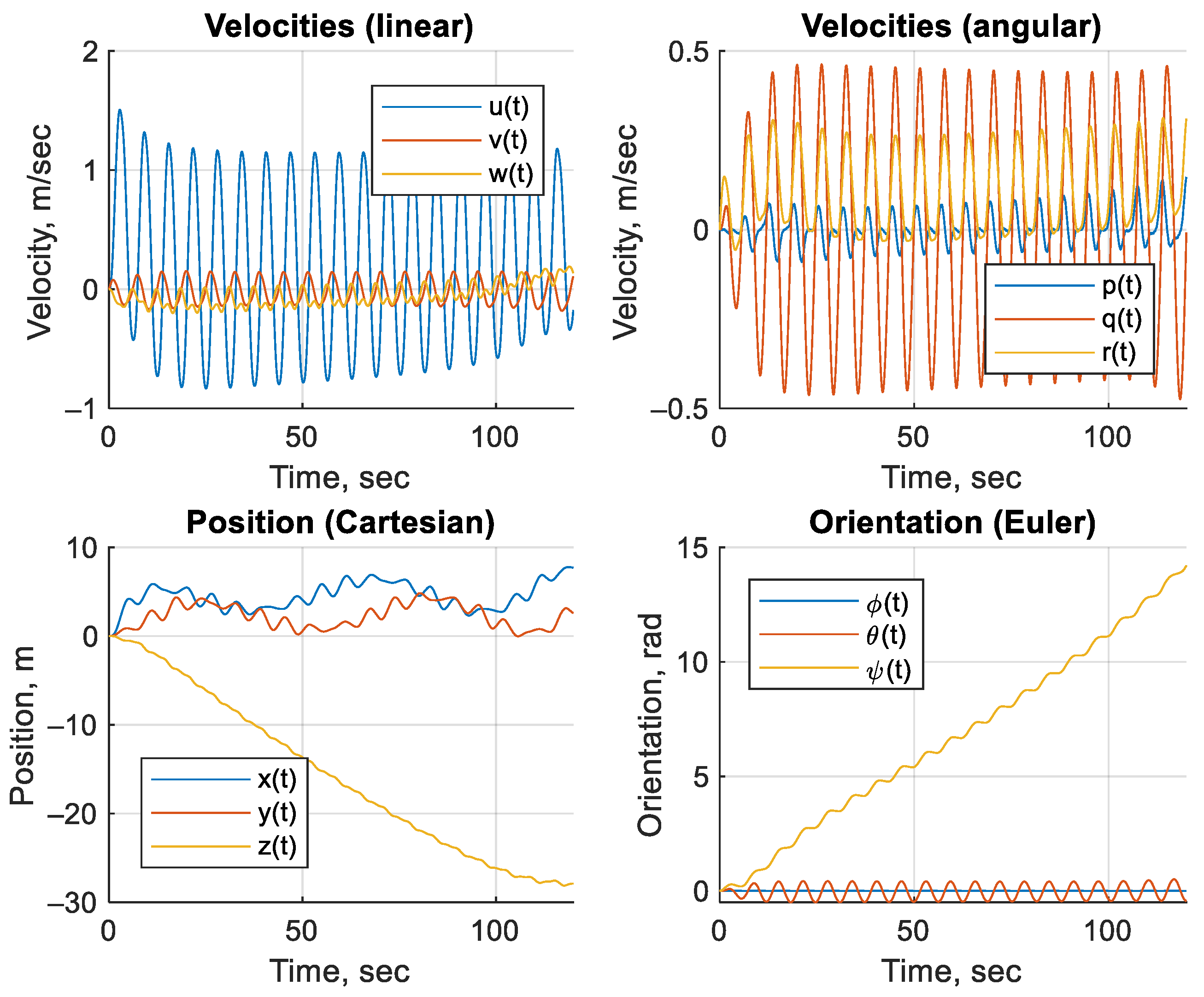
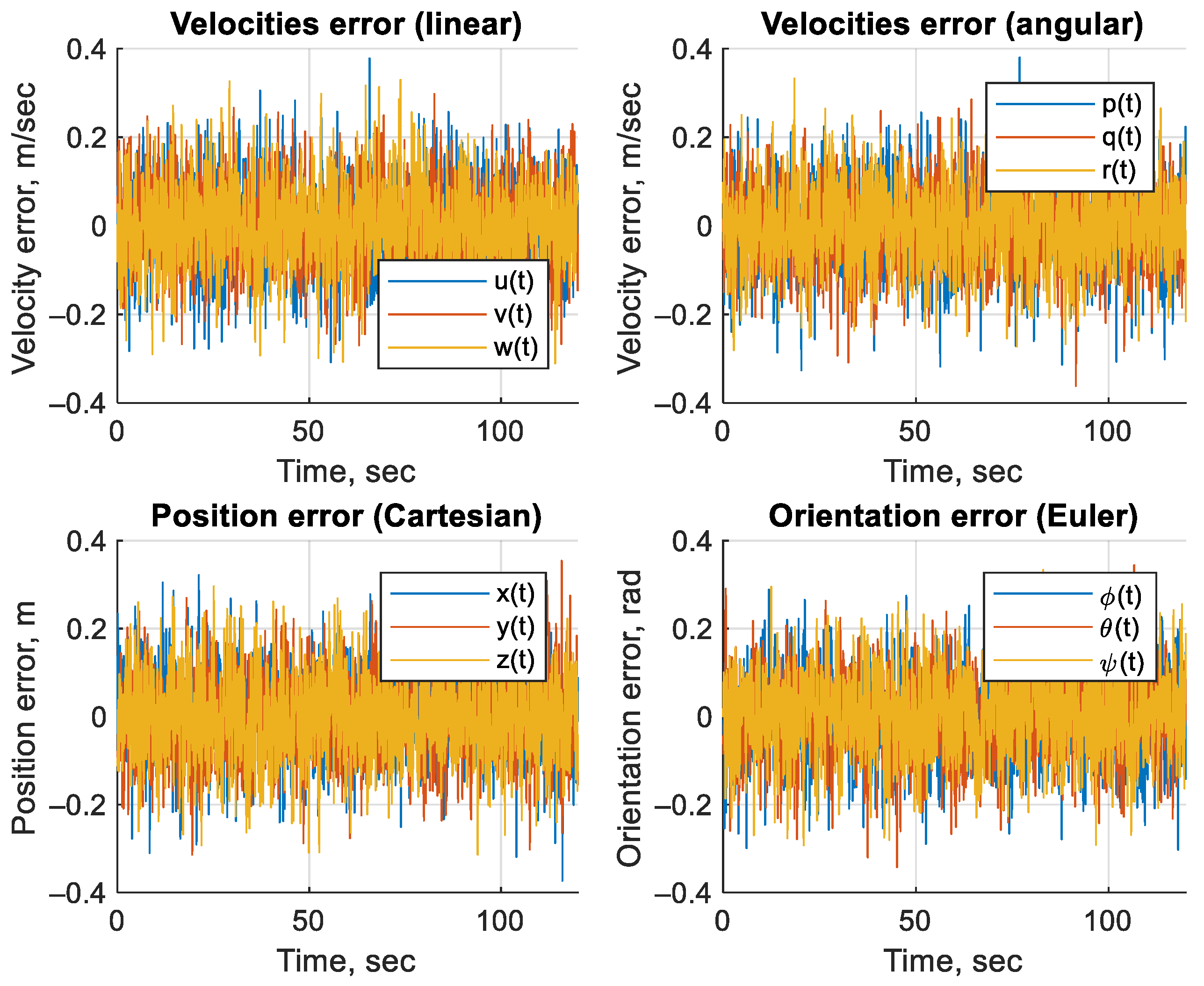
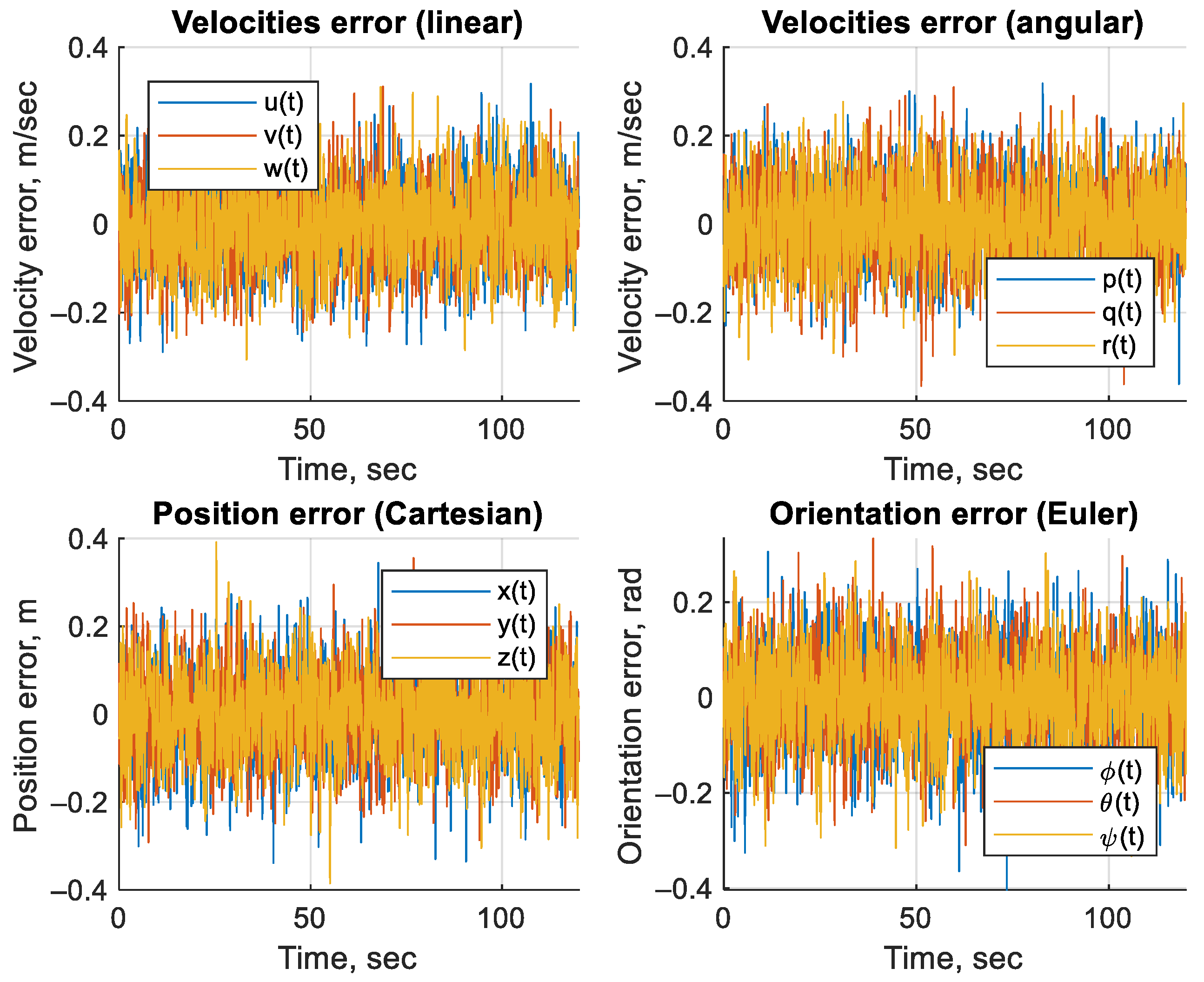
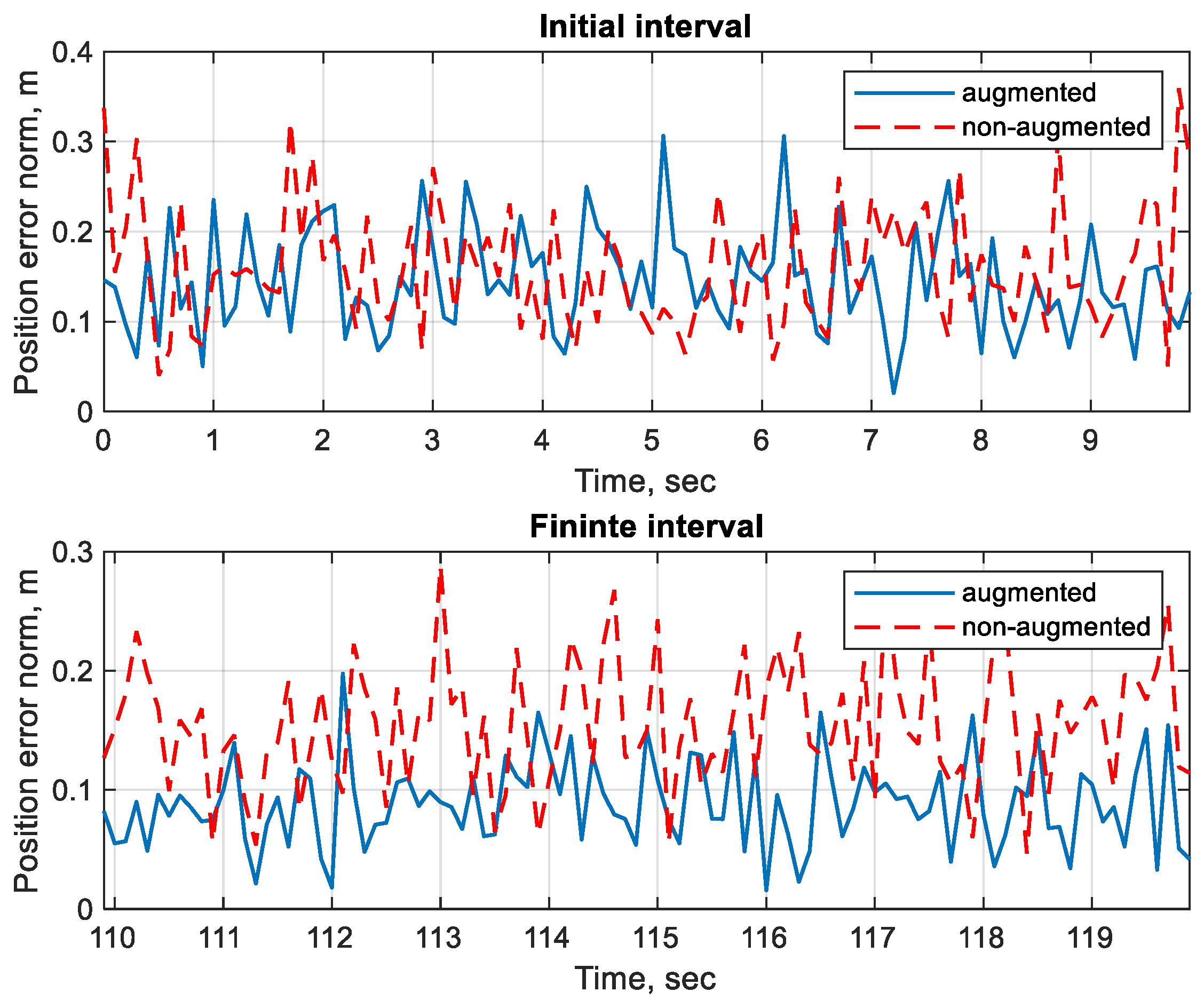
3. Results

Consider as an estimation object the MMT-300 submersible, which was considered in detail in [5]. To simulate the model uncertainties, the hydrodynamic parameters in the form of $M_A$, $C_A\left(\nu \right)$ and $D\left(\nu \right)$ from Equations (45) and (48) will be initially assumed to be equal to zero.

In the present work context, AUV control algorithms for emphasizing the state estimation will not be considered. Various harmonic combinations will be used as the control.

Consider that the AUV has both continuous and discrete measurement sensors (

Table 2. Update rates of the sensors.

Sensor	Update Rate	Measurements
IMU	50 Hz	${\nu }_1$, ${\nu }_2$, ${\eta }_2$
GPS	1 Hz	$x$, $y$
DVL	25 Hz	${\nu }_1$
PS	50 Hz	$z$

). If there is no corresponding continuous sensor for one measured discrete quantity, it is replaced by the ZOH for the discrete measurement. Also, in the following steps, all discrete measurers for the same quantity are brought to the largest update rate.

The correlations between discrete and continuous readings with noise parameters are shown in

Table 3. Sensor parameters.

Measurements	Continuous	Discrete
$x$	ZOH $~\mathcal{N}\left(0, 0.5\right)$	1 Hz $~\mathcal{N}\left(0, 0.5\right)$
$y$	ZOH $~\mathcal{N}\left(0, 0.5\right)$	1 Hz $~\mathcal{N}\left(0, 0.5\right)$
$z$	$~\mathcal{N}\left(0, 0.25\right)$	50 Hz $~\mathcal{N}\left(0, 0.1\right)$
$\varphi$	ZOH $~\mathcal{N}\left(0, 0.05\right)$	50 Hz $~\mathcal{N}\left(0, 0.05\right)$
$\theta$	ZOH $~\mathcal{N}\left(0, 0.05\right)$	50 Hz $~\mathcal{N}\left(0, 0.05\right)$
$\psi$	$~\mathcal{N}\left(0, 0.15\right)$	50 Hz $~\mathcal{N}\left(0, 0.05\right)$
$u$	$~\mathcal{N}\left(0, 0.1\right)$	25|50 Hz $~\mathcal{N}\left(0, 0.01\right)$
$v$	$~\mathcal{N}\left(0, 0.1\right)$	25|50 Hz $~\mathcal{N}\left(0, 0.01\right)$
$w$	$~\mathcal{N}\left(0, 0.1\right)$	25|50 Hz $~\mathcal{N}\left(0, 0.01\right)$
$p$	$\mathrm{ZOH} ~\mathcal{N}\left(0, 0.01\right)$	$50 \mathrm{Hz} ~\mathcal{N}\left(0, 0.01\right)$
$q$	$\mathrm{ZOH} ~\mathcal{N}\left(0, 0.01\right)$	$50 \mathrm{Hz} ~\mathcal{N}\left(0, 0.01\right)$
$r$	$\mathrm{ZOH} ~\mathcal{N}\left(0, 0.01\right)$	$50 \mathrm{Hz} ~\mathcal{N}\left(0, 0.01\right)$

. The accuracy differences in favor of discrete meters are also noticeable there.

For state estimation, the process-noise covariance matrix parameters $Q$ and measurement covariance matrices $R$ for the discrete and continuous filter components were chosen according to Table 3. The process noise for the augmented components in the state vector is assumed to be Gaussian, centered, and with large deviation $~\mathcal{N}\left(0, 100\right)$. For all other components, the process noise is assumed to be negligibly small.

The simulation results are presented below. The initial state of the underwater vehicle in this case is defined as zero. Figure 2 shows the trajectories of the submersible.

In this section, UKF with the scheme in Section 2.4 will be used to compare with the proposed approach. Figure 3 shows the estimation errors with the proposed method without taking into account the state vector augmentation by (47).

Figure 4 shows the estimation errors with the proposed method considering the state-vector augmentation. The benefit from augmentation can be seen here, providing better convergence.

The comparison between the proposed approach and hybrid UKF was performed using RMSE metric and summarized in

Table 4. Quality metrics.

Case	RMSE
Proposed Hybrid Kalman Filter
Non-augmentation	$\eta | \left[0.3907 0.3963 0.3910 0.3962 0.4004 0.4016\right]$
	$\nu | \left[0.3917 0.4028 0.4023 0.3989 0.3937 0.4004\right]$
Augmentation	$\eta | \left[0.3900 0.3991 0.3914 0.3875 0.3989 0.3990\right]$
	$\nu | \left[0.3920 0.3998 0.3993 0.3965 0.3997 0.3979\right]$
Hybrid Unscented Kalman Filter
Non-augmentation	$\eta | \left[0.5341 0.5299 0.7320 0.2454 0.5148 0.5530\right]$
	$\nu | \left[0.4552 0.6103 0.7928 0.4087 0.5383 0.5172\right]$
Augmentation	$\eta | \left[0.4823 0.4698 0.5479 0.3635 0.5116 0.5834\right]$
	$\nu | \left[0.4073 0.5431 0.6988 0.4735 0.5276 0.4995\right]$

. A minor advantage remained with the proposed approach. Moreover, the processing time taken by the proposed approach was 4.9910 s, while the UKF took 9.1316 s, which is almost twice as long. Even considering that the accuracy of UKF depends on the flexible fitting, the processing time will not decrease, which is a critical issue.

For non-augmented cases, the proposed approach achieves lower RMSE values across all state variables, particularly in linear and angular velocities, demonstrating its robustness. When state augmentation is applied, the improvement is even more pronounced, with RMSE reductions of up to 20% in some components.

From Figure 5, it is noticeable that at the initial interval of the position-estimation error norm ${‖{\eta }_1-{\widehat{\eta }}_1‖}_2$ almost does not differ between the augmented variant and the non-augmented variant. However, at the finite estimation interval, the augmented variant shows better results, which is evident from the lower graph amplitude, which is provided by the on-line hydrodynamic parameter estimation.

4. Discussion

The outcomes presented in this study demonstrate the proposed hybrid filtering algorithm’s effectiveness for the state estimation in autonomous underwater vehicles (AUVs) under discrete-continuous measurement applications. A comparison with the hybrid sigma-point Kalman filter (UKF) shows that the proposed method provides comparable or even higher accuracy at a lower computational cost. This is especially important for real-time systems where performance is a critical parameter.

Advantages and limitations of the proposed method:

• The state-vector augmentation was used to improve the estimation convergence, as evidenced by the reduction in errors (RMSE) compared to the method without augmentation. This is in agreement with previous studies such as [17,18,19,20,21,22], where augmentation was used to estimate hydrodynamic parameters.
• Like other Kalman filters, the proposed method is sensitive to the model precision. Unaccounted nonlinearities or significant deviations from the noise Gaussianity may reduce the estimation quality.
• The augmented state vector’s high dimensionality can increase the computational load, although this was balanced in this study by optimizing the algorithm.

In the further perspective, it is planned to extend the algorithm to work with more complex multi-rate systems, where measurements can be received not only with different frequencies but also with variable delays. This will require the new synchronization methods and weighting coefficient adaptation.

The proposed method assumes synchronized measurements for theoretical simplicity. In practice, minor asynchrony (e.g., timestamp mismatches within a sampling interval) is mitigated by: hold-and-predict strategy, when continuous measurements are held until the next discrete update, with the state propagated forward using the continuous model; buffering, when out-of-sequence discrete measurements are processed in batches, with the oldest data discarded if delays exceed a threshold.

For severe asynchrony, future work could integrate timestamp-based reweighting or asynchronous filter variants, though this is beyond the current scope.

Investigating the combination of the proposed method with other algorithms, such as particle filters (PF) or ensemble filters (EnKF), may allow to improve the accuracy under strong nonlinearities or model uncertainties.

The proposed filter, like all Kalman filters, assumes Gaussian noise and linear dynamics. While the proposed one does not explicitly consider non-Gaussian noise, its continuous-discrete formulation inherently smooths abrupt noise variations through integration over time intervals, mitigating the impact of outliers compared to purely discrete methods.

The augmented state vector introduces additional dimensionality, which can increase computational costs. To alleviate this problem, a sparse matrix strategy has been utilized where a block-diagonal structure of hydrodynamic parameter matrices is used, which allows sparse matrix operations to be performed efficiently, reducing memory space and computational cost.

The proposed filter’s computational efficiency advantage over the UKF stems from its analytical treatment of continuous-discrete fusion. The UKF relies on sigma-point sampling, which scales combinatorially with state dimension, whereas the proposed one directly propagates the covariance matrix using the Riccati equation.

The RMSE differences (Table 4) reflect the proposed filter tighter integration of continuous and discrete measurements, avoiding approximation errors introduced by sigma-point transformations in the UKF. The UKF’s flexibility in handling nonlinearities, however, may make it preferable in highly nonlinear regimes not addressed here.

The proposed algorithm can be adapted for use in other areas such as autonomous vehicles, robotics, and monitoring systems, where the problem of heterogeneous data compilation is also relevant.

Further research could focus on accounting for non-stationary measurement and process noise, which is especially important for operation in changing environmental conditions.

5. Conclusions

The research has resulted in the development and justification for the optimal state-estimation algorithm for discrete-continuous autonomous underwater vehicle (AUV) systems. The proposed approach demonstrates high efficiency in improving the accuracy and reliability in AUV state-parameter estimation by optimally combining data from different information sources.

The developed algorithm has a significant potential for application in a wide range of areas related to information processing in complex technical systems.

The proposed AHKF has three key limitations:

• Computational Load: State augmentation increases dimensionality, making the method less suitable for ultra-low-power embedded systems without hardware acceleration.
• Synchronization Assumption: The filter assumes perfectly synchronized continuous/discrete measurements. Performance may degrade with significant sensor latency.
• Nonlinearity Handling: Strong nonlinearities (e.g., complex noise, turbulent flow beyond quadratic damping) requires additional linearization steps, akin to EKF/UKF.

It is important to note that the proposed approach is flexible and scalable. It can be adapted to work with a large number of information sources, which allows extending its applicability to more complex systems. In addition, the algorithm can be modified for use in different discrete continuous systems without focusing on AUVs.

References

- Kramar, V.; Kabanov, A.; Alchakov, V. Multiloop Multirate Continuous-Discrete Drone Stabilization System: An Equivalent Single-Rate Model. Drones 2021, 5, 129. [Google Scholar] [CrossRef]
- Ju, C.; Son, H.I. A Hybrid Systems-Based Hierarchical Control Architecture for Heterogeneous Field Robot Teams. IEEE Trans. Cybern. 2023, 53, 1802–1815. [Google Scholar] [CrossRef] [PubMed]
- Fossen, T.I. Handbook of Marine Craft Hydrodynamics and Motion Control, 2nd ed.; Wiley: Hoboken, NJ, USA; Chichester, UK, 2021; ISBN 978-1-119-57503-0. [Google Scholar]
- Antonelli, G. Underwater Robots; Springer Tracts in Advanced Robotics; Springer International Publishing: Cham, Switzerland, 2018; Volume 123, ISBN 978-3-319-77898-3. [Google Scholar]
- Kramar, V.; Kabanov, A.; Dementiev, K. Autonomous Underwater Vehicle Navigation via Sensors Maximum-Ratio Combining in Absence of Bearing Angle Data. JMSE 2023, 11, 1847. [Google Scholar] [CrossRef]
- Scherbatyuk, A.F. Multiple AUV Navigation without Using Acoustic Beacons. Gyroscopy Navig. 2022, 13, 253–261. [Google Scholar] [CrossRef]
- Jeong, D.B.; Ko, N.Y. Sensor Fusion for Underwater Vehicle Navigation Compensating Misalignment Using Lie Theory. Sensors 2024, 24, 1653. [Google Scholar] [CrossRef]
- Filaretov, V.F.; Zhirabok, A.N.; Zyev, A.V.; Protsenko, A.A.; Tuphanov, I.E.; Scherbatyuk, A.F. Design and Investigation of Dead Reckoning System with Accommodation to Sensors Errors for Autonomous Underwater Vehicle. In Proceedings of the OCEANS 2015—MTS/IEEE Washington; IEEE: Washington, DC, USA, 2015; pp. 1–4. [Google Scholar]
- Yuan, X.; Martínez-Ortega, J.-F.; Fernández, J.; Eckert, M. AEKF-SLAM: A New Algorithm for Robotic Underwater Navigation. Sensors 2017, 17, 1174. [Google Scholar] [CrossRef]
- Merveille, F.F.R.; Jia, B.; Xu, Z.; Fred, B. Advancements in Sensor Fusion for Underwater SLAM: A Review on Enhanced Navigation and Environmental Perception. Sensors 2024, 24, 7490. [Google Scholar] [CrossRef]
- Luo, J.; Ko, H.-L. UKF-Based Inverted Ultra-Short Baseline SLAM With Current Compensation. IEEE Access 2022, 10, 67329–67337. [Google Scholar] [CrossRef]
- Mu, P.; Zhang, X.; Qin, P.; He, B. A Variational Bayesian-Based Simultaneous Localization and Mapping Method for Autonomous Underwater Vehicle Navigation. JMSE 2022, 10, 1563. [Google Scholar] [CrossRef]
- Liu, Q.; Li, M. Position Control for an Autonomous Underwater Vehicle under Noisy Conditions. Proc. Inst. Mech. Eng. Part I J. Syst. Control. Eng. 2022, 236, 1119–1132. [Google Scholar] [CrossRef]
- Liu, Q.; Li, M. Discrete-Time Position Control for Autonomous Underwater Vehicle under Noisy Conditions. Appl. Sci. 2021, 11, 5790. [Google Scholar] [CrossRef]
- Zhao, J.; Zhang, Y.; Li, S.; Wang, J.; Fang, L.; Ning, L.; Feng, J.; Zhang, J. An Improved Unscented Kalman Filter Applied to Positioning and Navigation of Autonomous Underwater Vehicles. Sensors 2025, 25, 551. [Google Scholar] [CrossRef] [PubMed]
- Zhang, A.; Wu, Y.; Zhi, C.; Yang, R. A Novel Adaptive Factor-Based H∞ Cubature Kalman Filter for Autonomous Underwater Vehicle. JMSE 2022, 10, 326. [Google Scholar] [CrossRef]
- Deng, F.; Levi, C.; Yin, H.; Duan, M. Identification of an Autonomous Underwater Vehicle Hydrodynamic Model Using Three Kalman Filters. Ocean. Eng. 2021, 229, 108962. [Google Scholar] [CrossRef]
- Sajedi, Y.; Bozorg, M. Robust Estimation of Hydrodynamic Coefficients of an AUV Using Kalman and H∞ Filters. Ocean. Eng. 2019, 182, 386–394. [Google Scholar] [CrossRef]
- Guan, Y.; Qin, H.; Hu, M.; Cui, Q.; Zheng, H.; Ding, R. Hydrodynamic Parameter Identification of Deep-Sea Mining Vehicle during Deployment and Retrieval Using a Nonlinear Filter. Adv. Theory Simul. 2024, 7, 2400066. [Google Scholar] [CrossRef]
- Shariati, H.; Moosavi, H.; Danesh, M. Application of Particle Filter Combined with Extended Kalman Filter in Model Identification of an Autonomous Underwater Vehicle Based on Experimental Data. Appl. Ocean. Res. 2019, 82, 32–40. [Google Scholar] [CrossRef]
- Sabet, M.T.; Daniali, H.M.; Fathi, A.; Alizadeh, E. Identification of an Autonomous Underwater Vehicle Hydrodynamic Model Using the Extended, Cubature, and Transformed Unscented Kalman Filter. IEEE J. Ocean. Eng. 2018, 43, 457–467. [Google Scholar] [CrossRef]
- Lu, S.; Wang, B.; Dong, Z.; Hu, Z.; Ding, Y.; Liu, W. Parameter Identification of an Unmanned Surface Vessel Nomoto Model Based on an Improved Extended Kalman Filter. Appl. Sci. 2024, 15, 161. [Google Scholar] [CrossRef]
- Shaukat, N.; Otero, P. Underwater Vehicle Positioning by Fuzzy and Neural Adaptive Kalman Sensor Fusion. In Proceedings of the OCEANS 2021: San Diego—Porto, San Diego, CA, USA, 20–23 September 2021; pp. 1–7. [Google Scholar]
- Shaukat, N.; Ali, A.; Javed Iqbal, M.; Moinuddin, M.; Otero, P. Multi-Sensor Fusion for Underwater Vehicle Localization by Augmentation of RBF Neural Network and Error-State Kalman Filter. Sensors 2021, 21, 1149. [Google Scholar] [CrossRef]
- Wang, Y.; Xie, C.; Liu, Y.; Zhu, J.; Qin, J. A Multi-Sensor Fusion Underwater Localization Method Based on Unscented Kalman Filter on Manifolds. Sensors 2024, 24, 6299. [Google Scholar] [CrossRef] [PubMed]
- Kulikov, G.Y.; Kulikova, M.V. State Estimation for Nonlinear Continuous–Discrete Stochastic Systems: Numerical Aspects and Implementation Issues; Studies in Systems, Decision and Control; Springer International Publishing: Cham, Switzerland, 2024; Volume 539, ISBN 978-3-031-61370-8. [Google Scholar]
- Shmaliy, Y.S.; Zhao, S. Optimal and Robust State Estimation: Finite Impulse Response (FIR) and Kalman Approaches, 1st ed.; Wiley: Hoboken, NJ, USA, 2022; ISBN 978-1-119-86307-6. [Google Scholar]
- Barfoot, T.D. State Estimation for Robotics, 2nd ed.; Cambridge University Press: Cambridge, UK, 2024; ISBN 978-1-009-29990-9. [Google Scholar]
- Potokar, E.; Norman, K.; Mangelson, J. Invariant Extended Kalman Filtering for Underwater Navigation. IEEE Robot. Autom. Lett. 2021, 6, 5792–5799. [Google Scholar] [CrossRef]
- Singh, R.K.; Saha, J.; Bhaumik, S. Maximum Correntropy Polynomial Chaos Kalman Filter for Underwater Navigation. Digit. Signal Process. 2024, 155, 104774. [Google Scholar] [CrossRef]
- Sheng, G.; Liu, X.; Sheng, Y.; Cheng, X.; Luo, H. Cooperative Navigation Algorithm of Extended Kalman Filter Based on Combined Observation for AUVs. Remote Sens. 2023, 15, 533. [Google Scholar] [CrossRef]
- Allotta, B.; Costanzi, R.; Fanelli, F.; Monni, N.; Paolucci, L.; Ridolfi, A. Sea Currents Estimation during AUV Navigation Using Unscented Kalman Filter. IFAC-PapersOnLine 2017, 50, 13668–13673. [Google Scholar] [CrossRef]
- Lewis, F.L.; Xie, L.; Popa, D. Optimal and Robust Estimation: With an Introduction to Stochastic Control Theory, 2nd ed.; Automation and Control Engineering; CRC Press: Boca Raton, FL, USA; Taylor & Francis Group: Abingdon, UK, 2008; ISBN 978-0-8493-9008-1. [Google Scholar]
- Tijjani, A.S.; Chemori, A.; Ali, S.A.; Creuze, V. Continuous–Discrete Observation-Based Robust Tracking Control of Underwater Vehicles: Design, Stability Analysis, and Experiments. IEEE Trans. Contr. Syst. Technol. 2023, 31, 1477–1492. [Google Scholar] [CrossRef]
- Särkkä, S.; Solin, A. On Continuous-Discrete Cubature Kalman Filtering. IFAC Proc. Vol. 2012, 45, 1221–1226. [Google Scholar] [CrossRef]
- Bhase, S.; Bhushan, M.; Kadu, S.; Mukhopadhyay, S. Continuous–Discrete Filtering Techniques for Estimating States of Nonlinear Differential–Algebraic Equations (DAEs) Systems. Int. J. Dynam. Control 2023, 11, 162–182. [Google Scholar] [CrossRef]
- Feddaoui, A.; Boizot, N.; Busvelle, E.; Hugel, V. High-Gain Extended Kalman Filter for Continuous-Discrete Systems with Asynchronous Measurements. Int. J. Control. 2020, 93, 2001–2014. [Google Scholar] [CrossRef]
- Kramar, V.; Alchakov, V.; Karapetian, V. The Models of Non-Stationary End Position Control Systems with Digital Corrective Circuits. In Proceedings of the 2023 International Conference on Ocean Studies (ICOS), Vladivostok, Russian, 3–6 October 2023; pp. 144–149. [Google Scholar] [CrossRef]
- Zhang, B.; Ji, D.; Liu, S.; Zhu, X.; Xu, W. Autonomous Underwater Vehicle Navigation: A Review. Ocean. Eng. 2023, 273, 113861. [Google Scholar] [CrossRef]
- Kumari, N.; Kulkarni, R.; Ahmed, M.R.; Kumar, N. Use of Kalman Filter and Its Variants in State Estimation: A Review. In Artificial Intelligence for a Sustainable Industry 4.0; Awasthi, S., Travieso-González, C.M., Sanyal, G., Kumar Singh, D., Eds.; Springer International Publishing: Cham, Switzerland, 2021; pp. 213–230. ISBN 978-3-030-77069-3. [Google Scholar]
- Jin, X.-B.; Robert Jeremiah, R.J.; Su, T.-L.; Bai, Y.-T.; Kong, J.-L. The New Trend of State Estimation: From Model-Driven to Hybrid-Driven Methods. Sensors 2021, 21, 2085. [Google Scholar] [CrossRef] [PubMed]
- Elfring, J.; Torta, E.; Van De Molengraft, R. Particle Filters: A Hands-On Tutorial. Sensors 2021, 21, 438. [Google Scholar] [CrossRef] [PubMed]
- Simon, D. Optimal State Estimation: Kalman, H∞, and Nonlinear Approaches, 1st ed.; Wiley: Hoboken, NJ, USA, 2006; ISBN 978-0-471-70858-2. [Google Scholar]
- Gao, Z. Cubature Kalman Filters for Nonlinear Continuous-Time Fractional-Order Systems with Uncorrelated and Correlated Noises. Nonlinear Dyn. 2019, 96, 1805–1817. [Google Scholar] [CrossRef]
- Urrea, C.; Agramonte, R. Kalman Filter: Historical Overview and Review of Its Use in Robotics 60 Years after Its Creation. J. Sens. 2021, 2021, 9674015. [Google Scholar] [CrossRef]
- Zorich, V.A. Mathematical Analysis II; Universitext; Springer: Berlin/Heidelberg, Germany, 2016; ISBN 978-3-662-48991-8. [Google Scholar]
- Alekseev, V.M.; Tihomirov, V.M.; Fomin, S.V. Optimal Control; Izd. 2, pererab. i dopoln.; Fizmatlit: Moskva, Russia, 2005; ISBN 978-5-9221-0589-7. [Google Scholar]
- Aström, K.J. Introduction to Stochastic Control Theory; Mathematics in Science and Engineering; Academic Press: New York, NY, USA, 1970; ISBN 978-0-12-065650-9. [Google Scholar]
- Casti, J. The Linear-Quadratic Control Problem: Some Recent Results and Outstanding Problems. SIAM Rev. 1980, 22, 459–485. [Google Scholar] [CrossRef]
- Zelikin, M.I. Optimalʹnoe Upravlenie i Variacionnoe Isčislenie; Izd. 2., ispr. i dop.; URSS: Moskva, Russia, 2004; ISBN 978-5-354-00622-9. [Google Scholar]