Abstract
To study the response of a flexible offshore floating photovoltaic (FPV) array under waves and a current, a numerical model is established using OrcaFlex. The effects of different waves and currents, as well as their coupled effects on the motion response of the offshore PFV array and the tension in the connectors and moorings under different static tensions, are investigated. Differences are illustrated between the responses of the buoys at different positions and under different moorings under the wave. With the relaxed moorings, the surge response of the buoy facing the wave increased by 159.3% compared with the buoy facing away from the wave. The current causes the overall drift of the array, which greatly influences the buoys facing the current. The mooring tension facing the wave restricts the motion of the buoys under the same direction as the wave and current, which shows that the trend of the buoys’ responses with the wave decreases with the increase in the current velocity, as the pitch reduces to 76.9% under relaxed moorings. There is a significant difference between the results obtained by the superposition summation wave and current loads and the ones of the combined wave–current. With the increase in the wave–current angle, the response is increased by 348.2% as the constraint of the moorings and the connectors is weakened.
1. Introduction
To ensure the stability of the energy supply and reduce the dependence on fossil fuels, the development and utilization of solar energy is particularly important. A photovoltaic is a power generation system that directly converts solar energy into electrical energy. The application and development of photovoltaic technology is an indispensable part of the energy revolution. Floating photovoltaics (FPVs) [1] are one of the most important parts of marine resource development and equipment utilization, which has a great development potential. According to the data in ‘Global Market Outlook for Solar Power/2023–2027’ by Solar Power Europe, the installed global photovoltaic capacity will reach 617 GW in 2027.
After the ground photovoltaic (GPV) and rooftop photovoltaic (RPV), the FPV is an emerging driver in the photovoltaic market. The offshore floating photovoltaic (FPV) is an important part of the equipment for developing and utilizing marine resources, and it has an excellent potential for growth in the future. It will cooperate with other marine equipment to provide services for marine transportation [2] and marine resource development [3].
However, compared with the GPV and RPV in the terrestrial environment and the FPV on inland water, the offshore FPV system will have to withstand more complex environmental loads, mainly wind, waves, and currents, which are the important factors causing difficulties in the design and manufacture of offshore FPV systems, including the high costs of installation and maintenance.
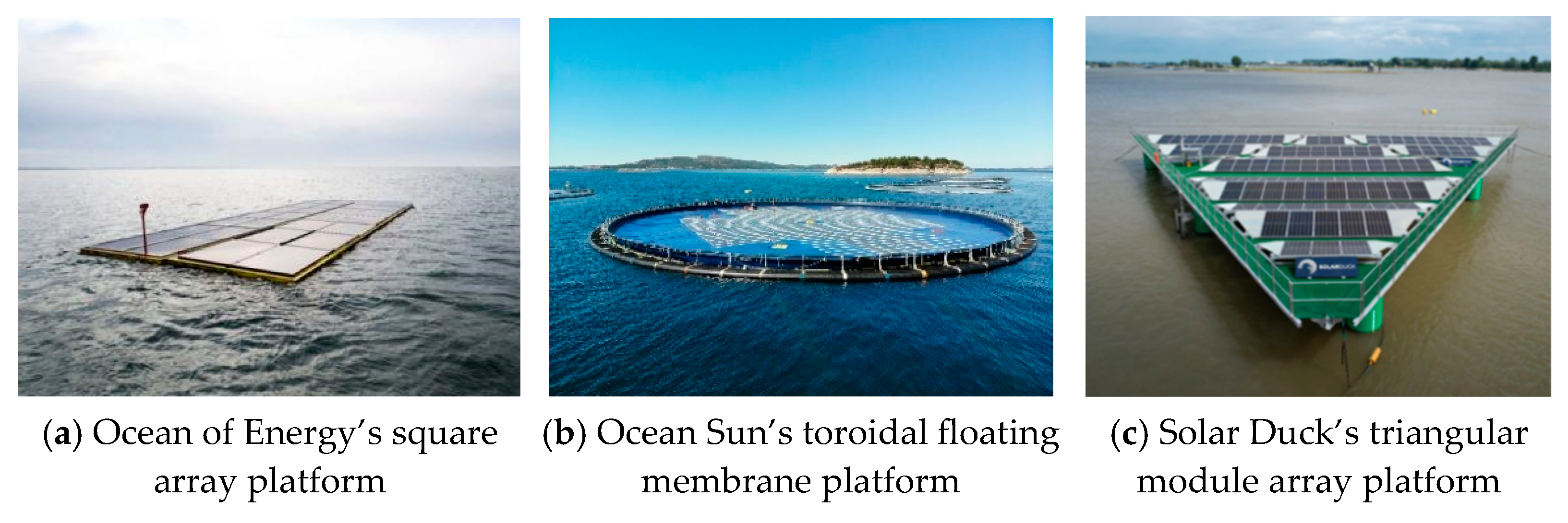
A typical FPV station covers a large sea area to increase power generation. It comprises photovoltaic modules, electronic equipment, brackets, floating bodies, and mooring lines. According to the shape of the floating body array, there may be three types of offshore FPVs [1]. The first is a floating array composed of multiple modular square float bodies. Each of the two modules are linked by connectors, which will make up the whole FPV station. Relative motions may happen between modules. The Zon op Zee [4] project about the multiple modular FPV has been developed by the Ocean of Energy in the North Sea near the Netherlands, as shown in Figure 1a. The connectors between the modules are hinged. However, it should be noted that for large floating bodies, the relative motion of this connection will induce complicated loads, leading to strength damage in the connection parts [5]. The second is a toroidal floating body composed of a circular cross-sectional floating body. The buoyancy ring is tightened by a high-strength flexible film made of special materials resistant to the marine environment. The photovoltaic panel is installed on the film, so the entire system can move with the waves.

Figure 1.
Three floating photovoltaic platforms with different shapes.
A 500 kW offshore FPV station in the Shandong Peninsula has been constructed using the elastic film platform technology [6] by the Norwegian Ocean Sun Company, as shown in Figure 1b. However, the film was filled with water due to the high wave height in the Yantai sea area. As the film platform was not equipped with a pump to pull out seawater, the heavy water led to the failure of the connection between the buoyancy ring and the film, resulting in the sinking of the film and components to the sea bottom.
Another system has cylinder bodies connected by rigid connectors, which are equipped with a floating system of photovoltaic panels. It has been developed and successfully placed in the sea of South Korea [7]. The connector used in this research is made of a fiber-reinforced plastic (FRP) composite material. The working efficiency of the cylinder-film type has been validated in South Korea’s seas. A triangular column-stabilized platform was also introduced, as shown in Figure 1c. The modular triangular rigid modules are flexibly connected together through flexible connections to form a large platform. It was tested by the Dutch developer Solar Duck, with a 65 kW photovoltaic array called King Eider in the inland bay of the Netherlands [8].
This type of platform was designed similarly to semi-submersible oil platforms but was manufactured with aluminum to be lightweight. The freeboard is more than 3 m above the water surface, which avoids contact with seawater on the photovoltaic module. The third type is the best one, with an excellent stability and seakeeping performance, but with more than dozens of times the cost.
The layouts need to be chosen reasonably according to the actual working environment and the carrying situation of the photovoltaic modules, also considering the balance of the cost and stability. Because the buoy’s motion will not affect the power generation of the FPV significantly, the stability of buoys is a non-sensitivity factor. A flexible but low-cost layout may focus more on the Intertidal Zone or offshore area, which is a few meters deep. However, a more flexible layout, resulting in enhanced movement, may cause the structure to be damaged in harsh marine environments.
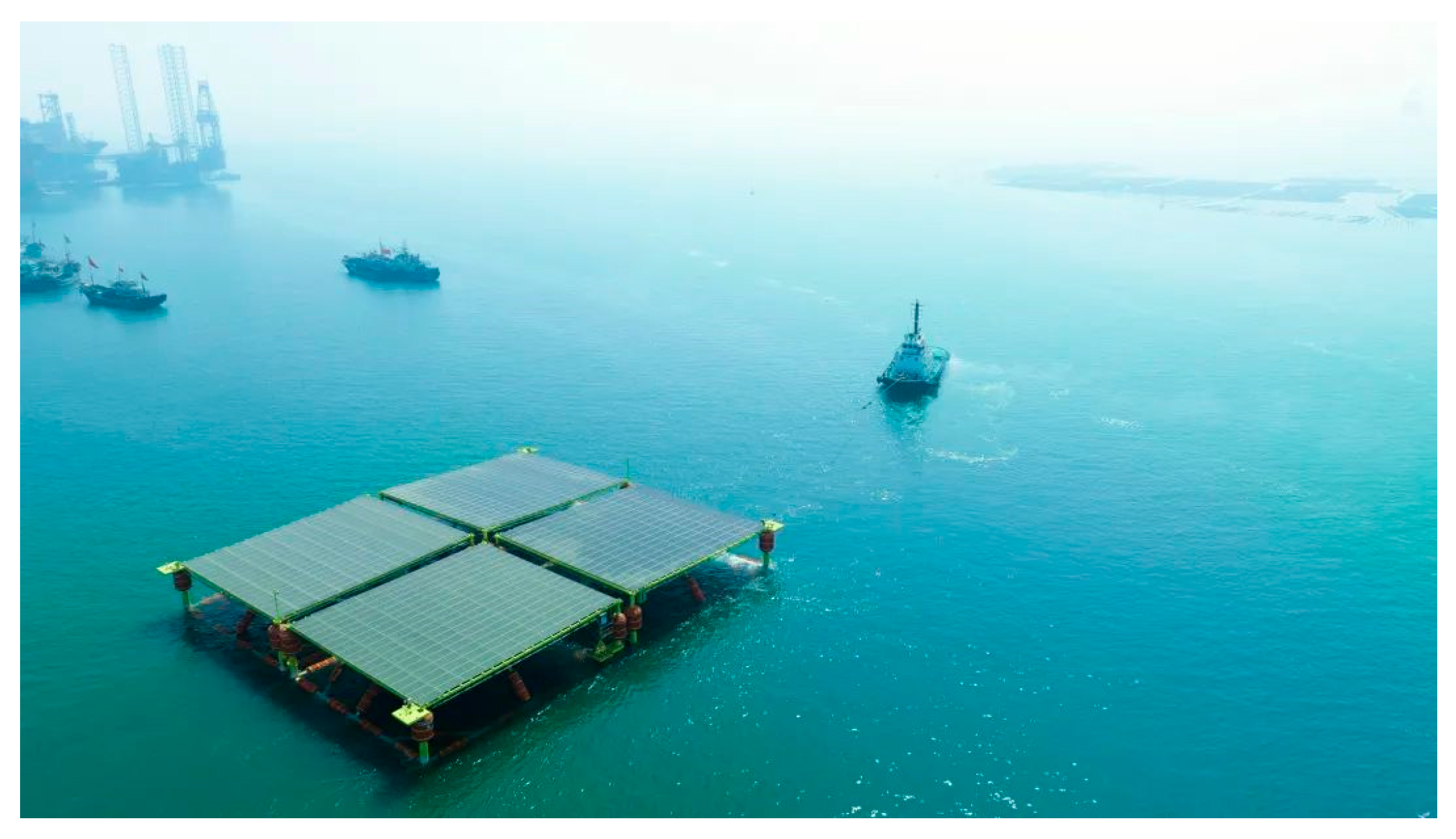
A semi-submersible offshore FPV power generation platform built by CIMC RAFFLES in 2023 is composed of four single floating buoys square arrays [9]. Its installation provides valuable experience through its comprehensive demonstration of the key factors, such as the power generation efficiency and the wind and wave resistance of each group of photovoltaic products’ photovoltaic platforms, as shown in Figure 2.
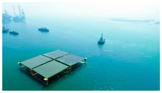
Figure 2.
The semi-submersible offshore FPV of CIMC RAFFLES.
Compared with traditional offshore platforms, the key problems are the multi-body hydrodynamics, a large number of mooring lines placed in different places, and connections between a large number of buoys. Several researchers have addressed the motion response analysis of multiple floating bodies under hydrodynamics. The motion response in the frequency domain is achieved by Newman [10] using the direct modal method to investigate the interaction between waves and hinged and fixed multi-floating bodies. Combining the HOBEM (High Order Boundary Element Method) with the generalized modal method, the motion of multiple ships moored side by side is studied by Hong et al. [11]. The hydro-elastic method is used to investigate the influence of the elastic stiffness of the floating body on the motion response of the multi-floating system by Lee and Newman [12]. For the multi-body floating piers, the motion of multi-body models connected by flexible and rigid connectors is predicted by [13] using the three-dimensional diffraction theory. Based on the three-dimensional potential flow theory, the motion response of side-by-side FPSO (floating production storage and offloading) systems is simulated by Qian et al. [14], and the relative motion results are obtained under the action of different mooring materials. A similar study was conducted by Pessoa et al. [15]. For hinged floats, Bispo et al. [16] analyzed the influence of different design parameters of mooring articulated VLFSs (Very Large Floating Structures) on the wave height and wave force under Airy and second-order Stokes waves. The connector loads of a three-module VLFS are investigated by experimental and numerical methods deployed in shallow water areas [17], showing that attention should be paid to the longitudinal loads. The differences in the motion response of the floating body with different structural parameters under the hydrodynamic action have been studied in this research, but less for the interaction between the various structures within the multi-floating body system.
To ensure the hydrodynamic performance of offshore FPVs and adapt to the complex and changeable marine environment, it is particularly important to develop key mooring schemes, such as the mooring type and mooring arrangement for offshore FPVs with a shallow draft and numerous floating bodies, which is comparable with the mooring of other energy converters operating in similar water depths [18]. The mooring system is divided into catenary, tension, and hybrid line types [19] and can utilize steel catenary chains or pre-stressed elastic ropes attached to the material. Different mooring systems have different working principles. Considering that the offshore FPV belongs to the multi-floating body structure, the number of floating bodies is large and many moorings are used. Ormberg and Larsen [20] pointed out that an uncoupled analysis may produce serious inaccurate results and proposed an overall coupled dynamics analysis method for floating/mooring/riser systems. Therefore, the coupling effect of each structure in a flexible multi-buoy offshore floating photovoltaic array cannot be ignored. With the development and utilization of new energy, more and more researchers are focusing on the motion of offshore FPVs under environmental loads; the interaction between the floating body and the mooring is also taken seriously. The fluid–solid coupling of a traditional fiber-reinforced plastic and HDPE (high-density polyethylene) floating tube is studied by Kim et al. [21] using linear wave theory.
The computational fluid dynamics (CFD) analysis shows that the structure has a certain influence on the frontal wave, and the maximum effective stress appears in the vertical and horizontal components of the front of the structure and when the wave crest passes through the multi-buoy structure. The hydrodynamics of a flexible thin-film PV array were analyzed by the computational fluid dynamics method in regular waves by Trapani and Millar [22]. Then, a series of experiments were performed on a toroidal floating membrane platform (thin-film PV), similar to Ocean Sun’s product, in a wave tank, as the connectors are elastic or rigid [23,24]. Using the CFD method, the multi-point mooring characteristics of the floating square array in a floating photovoltaic power station are obtained by Kong [25], and the influence of the offset, horizontal span, and number of mooring lines on the mooring tension have been considered.
Liang et al. [26] used the NSGA-II algorithm to obtain the simplified line length, axial stiffness, and submerged mass by iterations to achieve static restoring forces that were equivalent to the original. It was proposed for a very large floating structure’s scale model experiment; the simplified mooring system demonstrated its effectiveness by numerical studies and was verified by tests [27]. Numerical simulations for a global array of connected modular floaters were performed by Sree et al. [28] using the fluid–structure interaction method. Mohapatra and Guedes Soares [29] studied an array of floating or submersible flexible cages with mooring lines and without mooring lines. The above research associates the multi-floating system with the mooring system, studies the coupling between them, and proves that the influence between the multi-floating system and its mooring system is not negligible.
So far, the offshore FPV is a new technology that is still in the early stages of development [30]; the research literature and technical data are limited, and the design and installation have no industry standard. Therefore, many research gaps remain to be filled in the hydrodynamics, aerodynamics, aero-hydro-elastic coupling, and dynamic modeling of such structures and the design of mooring lines [31]. At the same time, with the wide applicability of offshore FPVs, they will be installed in a more complex flow field and designed according to the conventional typical environment, which cannot yet adapt to very harsh marine environments, such as typhoons, which makes it hard to guarantee the safe operation of marine FPVs in the whole life cycle.
In this paper, the flexible multi-buoy offshore floating photovoltaic (FPV) array consists of 84 buoys connected by a large number of connectors, an unprecedented design. Compared with the multi-floating structures mentioned above, such as the FPSO system with a shuttle tank and floating prier, the influence of hydrodynamics on the structure in the array will be more complicated. It is difficult to determine the multiple responses in the array with only the CFD method. Therefore, the FPV array model was established by OrcaFlex 11.0 and verified by experiments. The nonlinear coupled motion response, acceleration, connector tension, and mooring tension of different buoys in the offshore FPV array are analyzed, and the influence of the waves and current and their interactions on buoys and connectors at different positions are also included. This paper provides a reference for the large-scale design of FPV structures.
2. Geometry and Environment
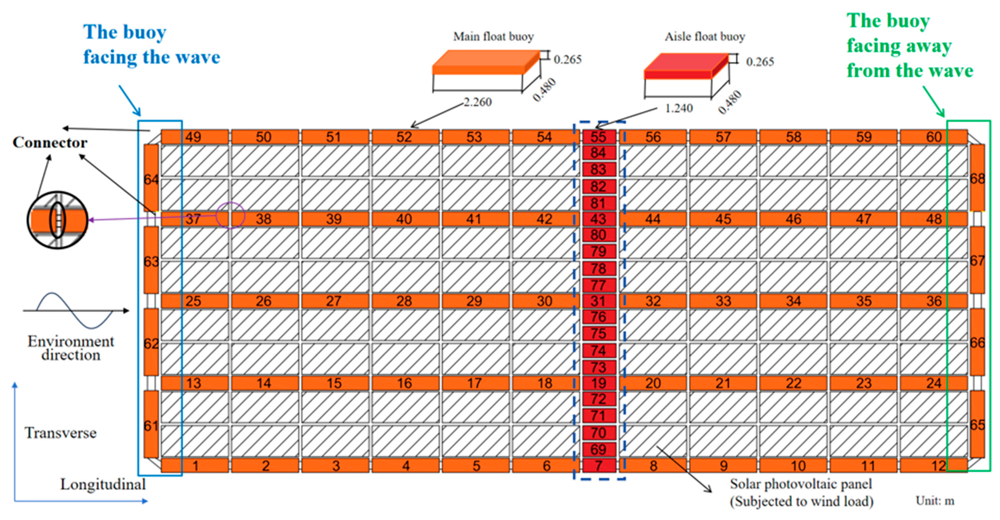
One type of multi-buoy offshore FPV array, shown in Figure 3, is introduced to investigate the hydrodynamics. The system is composed of 84 buoys connected to each other using connectors. Solar photovoltaic panels are fixed on the buoys. Due to the buoy’s small size, it is assumed to be a rigid body in the FPV array, ignoring any flexible deformation.
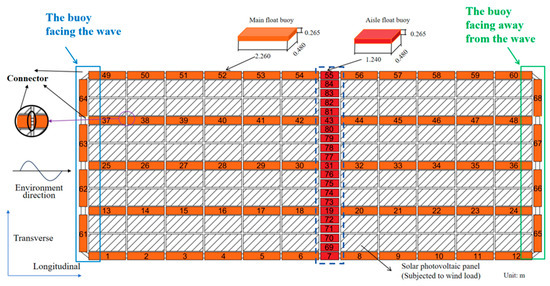
Figure 3.
Shape parameters and array arrangement of buoys.
2.1. Geometrics of Offshore FPV Buoy
2.1.1. Main Dimensions
The buoys are designed to have a square section connected in a square layout, as shown in Figure 3. Their shape was chosen to be easily manufactured to reduce costs. The photovoltaic panels were fixed with steel beams and columns between two adjacent buoys, such as buoy 37 and 49. The length of the multi-buoy FPV array is 27.84 m, and the width is 13.05 m. The array is composed of horizontal and vertical main floating buoys of the same size but has aisle floating buoys with slightly smaller lengths. The geometric parameters of the main and aisle buoys are also listed in Table 1.

Table 1.
Size of buoy.
The height of the buoys is small, not considering the wave height, as the low freeboard type withstands green water loads. It is designed to provide buoyancy to the light solar photovoltaic panels. As the waves pass through the FPV, the buoys may be immersed. However, the solar photovoltaic panels will not be damaged by the wave and the current. The buoys with a small length and width are designed to resist the wave load. After the wave passes through, the buoys will float in the water. Due to the connecter of the buoys, the whole FPV may experience an oscillatory motion. The multi-buoy FPV array is a flexible platform to avoid the wave load as the large buoy will result in a large wave load, which will increase the cost substantially.
2.1.2. Connector
The buoys in the offshore FPV array are linked through connectors, as shown in Figure 3. The transverse floating buoys are connected by two connectors and the longitudinal by three. The transverse buoys and the longitudinal buoys at the periphery of the array are connected by two connectors at the corner. The connection between the connector and the buoy does not withstand bending and torsional stiffness for the longitudinal buoy connector. The parameters of the connectors are shown in Table 2.
Table 2.
Parameters of mooring line arrangement.
2.1.3. Mooring of Offshore FPV
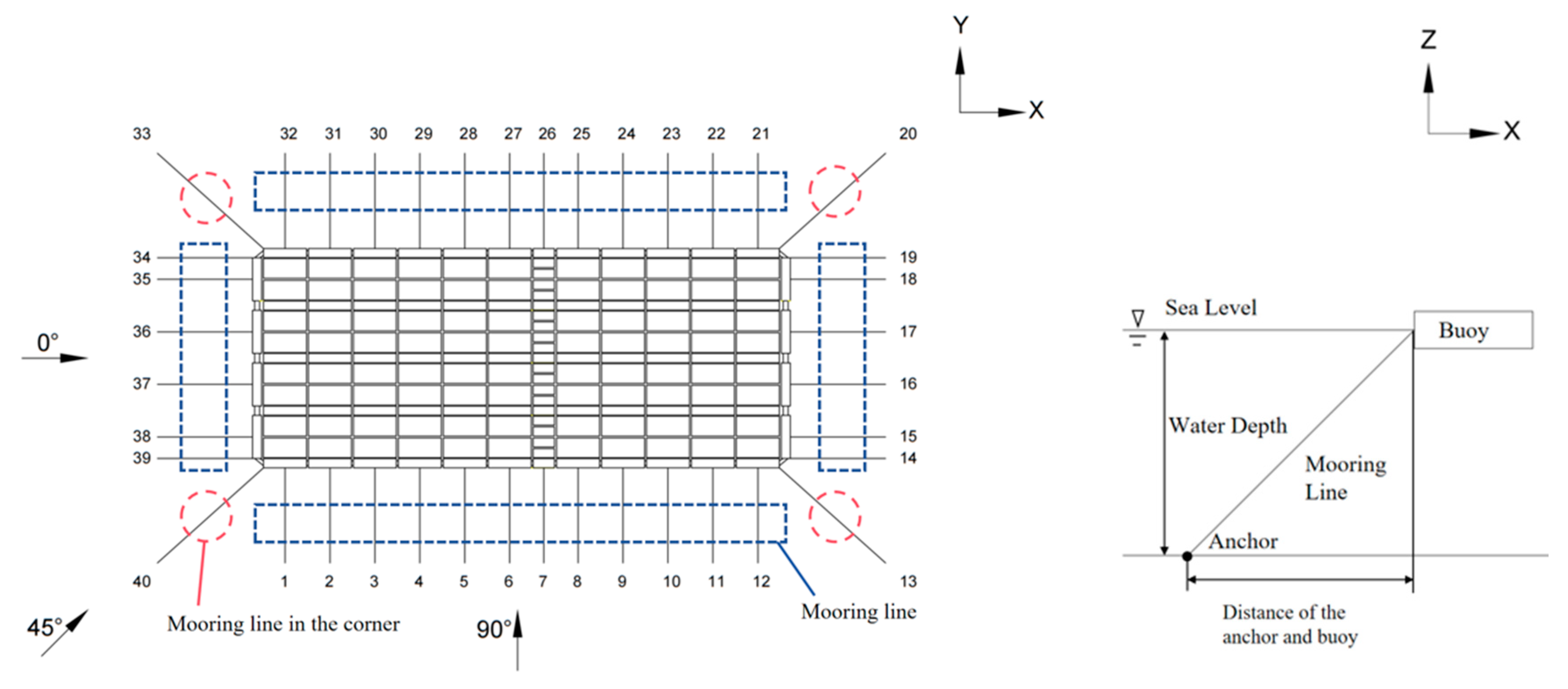
Multi-point mooring placed on different buoys is used to fix the offshore FPV array with 40 mooring lines. One end of the mooring line is connected to the buoy in the main buoy of the square array, and the other is connected to the anchor point. The mooring lines are evenly and symmetrically distributed around the FPV array, with four lines arranged in the corners, as shown in Figure 4. The mooring lines’ stiffness are shown in Table 3.
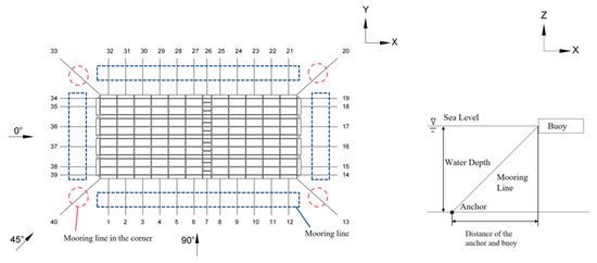
Figure 4.
Mooring arrangement diagram.
Table 3.
Stiffness of mooring lines.
The effective tension Te of the mooring increases with the increase in the water depth but decreases with the increase in mooring length by the static analysis [32]. The results are the largest for the case of the water depth of 18 m with a mooring line length of 27 m and the smallest for the water depth of 12 m with a mooring of 30 m. The effective mooring tension changes with one variable: water depth or mooring length. The relationship between the two factors and the effective tension is described by the regression method. A series of different polynomials are used to fit the nonlinear relationship, as listed in Table 4. Where d is the water depth and lm is the length of the mooring. The quadratic with cross terms can fit the relationship best, with the maximum correlation coefficient and minimum estimated error variance. For the relationship between the effective tension and water depth, the mooring line length is illustrated in Figure 5.
Table 4.
List of fitting results.
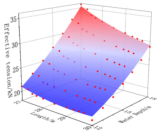
Figure 5.
Data and regression function.
Three water depth and mooring length combinations are selected to study the FPV’s response in different tension levels, as listed in Table 5. Com-I has the largest effective mooring tension, Com-III has the smallest mooring tension, and Com-II has the middle-level mooring tension.
Table 5.
Mooring tension levels.
2.2. Environment Parameters
2.2.1. Wave Parameters
The FPV is designed for use in the offshore waters of Fujian Province, China. According to the local environmental data, the wave period is 4.2–9.8 s, with an average height of 1.2 m. Regular waves with wave periods of 4.0 s, 5.0 s, 6.0 s, 7.0 s, and 8.0 s are used to explore the effect of waves on the buoy. The wave heights are selected as 0.8 m, 1.0 m, 1.2 m, 1.4 m, and 1.6 m.
Based on the linear superposition principle, the results of irregular oceans can be obtained by the linear superposition of regular waves under stable control conditions. Therefore, in order to study the interaction between waves and floating bodies, the regular waves have been adopted as the waves in the environments where the floating bodies are located.
The free-surface can be expressed by a function as follows:
The velocity potential Φ (x, y, z, and t) can be used to describe the fluid velocity vector of time at the points in a Cartesian coordinate system fixed in space. According to the law of the conservation of energy, the velocity potential has to satisfy the Laplace equation [31]. Considering the non-permeability of the seabed and the dynamic and kinematic conditions of the free-surface, the boundary condition equation can be obtained:
Taylor expansion can transfer the free-surface conditions from the free-surface position to the mean free-surface at z = 0. Using the perturbation method the velocity potential function is as follows:
where , , ……, are the nth-order velocity potential.
The linear wave dispersion relation formula of finite water depth is [33]
where L is wavelength; T is the wave period; k is the wave number; and is the wave frequency.
The dispersion relationship of the third-order and fifth Stokes wave theory is different from those for the first wave, whose wavelengths are calculated by Equations (9) and (10) [34].
where H is the wave height. The parameters C1 and C2 are obtained as follows:
The relationship of the wavelength, water depth, wave height, and period are described by the dispersion equations. The wavelength of each water depth and period can be obtained by an iterative numerical solution for the linear and nonlinear waves. Based on the wave characteristics, such as d/L and H/L, the applicability of the waves theory is confirmed. If the wave steepness H/L is small, the small amplitude assumption is hence valid for the linear wave [35]. If the linear wave is not applicable, the nonlinear wave as a fifth-order Stokes wave is set in OrcaFlex.
The calculation results show that the wavelengths of the same period are different in the water depth range of a tidal range change, but the difference is not large. The maximum chang range of the wave is in the period of 8.0 s, the wavelengths’ change is 10.49 m, and the change rate is 12.91%. And the minimum change range is in the period of 4.0 s, the wavelengths’ change is 0.11 m, and the change rate is 0.44%.
Since the wavelengths between different water depths in the same period do not change much, the average water depth wavelengths are taken as the reference wavelengths to study the influence of the degree of mooring tension on the mooring lines and the motion response of the offshore FPV during the period change.
2.2.2. Current Parameters
The current caused by tidal fluctuation is usually 0.01–1 m/s, even reaching more than 2 m/s in special areas. Under the current action, the offshore FPV will experience a large drift motion. To reasonably plan the installation position of the FPV and avoid the collision of the FPV with other marine structures, different velocities are adopted to analyze the current’s influence on the FPV mooring tension and motion.
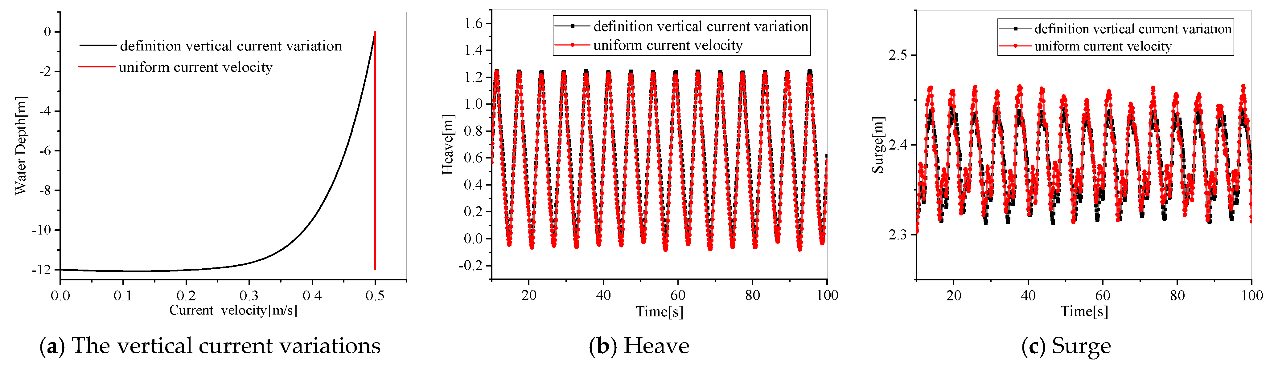
Currents often occur in open seas. Currents on the surface of the ocean are mainly caused by winds, the changes in pressure, and tides acting on the sea surface. Under the condition of a large tidal range, the currents caused by the rise and fall of the tides are usually 0.01–1 m/s, and can even reach more than 2 m/s in special sea areas. A complex flow field with a time-varying velocity direction can be formed with other currents. In the natural environment, it is mostly an unsteady flow. For example, in the process of tidal fluctuation, the seawater flow rate, water depth, and bottom friction velocity change with time, and this change is not synchronized. However, in this study, the draft of the buoy is only 0.11 m, which is relatively shallow. It is mainly affected by the surface flow of the sea surface. Therefore, the current velocity of the sea surface is the main concern. The current below the water surface mainly affects the mooring of the FPV array. The uniform currents are set in this paper, as the current velocity changed in the vertical profile. Comparing the motion response of the buoy under different vertical current variations, the difference is small, as shown in Figure 6. Therefore, in order to simplify this study, it is treated as a steady flow.
Figure 6.
The motion response of the buoy in different vertical current variations.
2.2.3. Wave–Current Coupling
When the wave is superimposed with the steady flow, the calculation results of the wave motion value and the related load need to be corrected. The wave period is corrected from the velocity of the free flow to the performance period. The current in the same direction of the wave lengthens the wavelength and in the opposite direction shortens the wavelength [33]. The amplitude also varies at the same time [36]. Therefore, the horizontal velocity of the water points considering the wave–current interaction and not considering the wave–current interaction is different. In this paper, the effective tension of the mooring under the wave and the current on the FPV array are superimposed, and the effective tension of the mooring under the wave and current is compared. And the difference is compared under different combinations of the water depth and mooring length.
2.2.4. Wind Parameters
The solar photovoltaic panels of the FPV array will be mainly exposed to wind. The height of the buoy is low, and the wind area is limited. Therefore, the force from the wind is 9 m/s by the photovoltaic panel and is simplified as a value to be added in the model, by adding an applied load on the buoy. The variations in the wind load in the response were not discussed.
To reveal the multi-array FPV’s hydrodynamic characteristics, only the environment direction of 0° is investigated, with the same direction of the wind and waves, as shown in Figure 4.
3. Computation and Simulation
3.1. Model Establishment
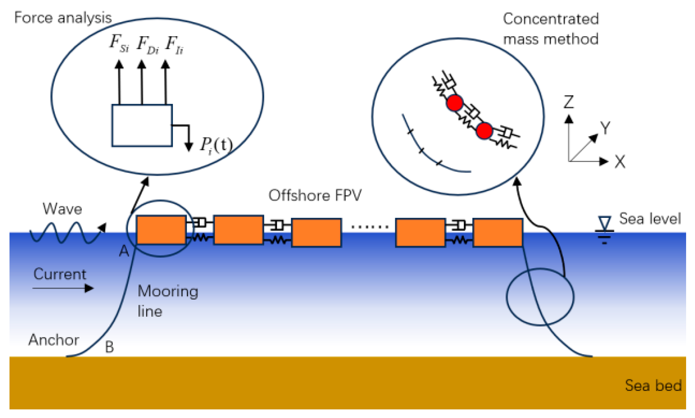
The multiple buoys, with six degrees of freedom, are connected by line units using OrcaFlex to form the buoy array of the offshore FPV, as shown in Figure 3. The hydrodynamics model of the FPV is shown in Figure 7. The red components are the multiple buoys connected, and the green ones are the solar photovoltaic panels. The offshore FPV moorings and connectors are established using line elements. The moorings are used to connect the buoys with the seabed by anchoring, which is almost completely immersed in the water, while the connectors link the buoys.
Figure 7.
The FPV hydrodynamics model.
3.2. Theory of Hydrodynamic Loads in Orcaflex
The numerical model of the FPV array in OrcaFlex is composed by Buoy and Line. The Buoy and the Line in OrcaFlex calculate the hydrodynamic load, which was the extended form of the Morison equation. This equation was originally proposed by Morison et al. [37] to calculate the wave load on a fixed vertical cylinder, which is suitable for structures with D/L < 0.2. In this study, the maximum drag width D of Buoy is 2.31 m, and the shortest wavelength is 24.95 m. Therefore, within the scope of this study, D/L = 0.09 < 0.2, which meets the theoretically applicable conditions.
The same principle can also be applied to moving objects. In this case, the inertial term reduces the amount of , and the resistance term uses the relative velocity of the object, thus obtaining the extended form of the Morison equation we used in OrcaFlex. It is also the most general form of the equation used in OrcaFlex [38].
where is the fluid force on the body, is the inertia coefficient for the body, is the mass of fluid displaced by the body, is the fluid acceleration relative to Earth, is the drag coefficient for the body, is the drag area, and is the fluid velocity relative to Earth.
3.3. Mechanical Analysis of Multi-Buoy Array Based on Multi-Body Dynamics
As the offshore FPV is composed of multiple floating bodies, there are a large number of moorings and connectors. The hydrodynamic response may be very complex under a combination of waves and currents, as every buoy will move in six degrees of freedom: surge, sway, heave, pitch, roll, and yaw. The adjacent buoys may interact with each other, and while the connector between the buoys is elastic, it will have both spreading and buffering effects on the load.
The i-th buoy of the offshore FPV is separated from the whole model. It will be subject to inertial, elastic restoring, damping, and interference forces, shown in Figure 8. Due to the static equilibrium position of the dynamic system, it is obtained as follows:
where is the elastic force opposite to the displacement direction, and is the stiffness coefficient, including the water elastic coefficient, the elastic restoring force coefficient, and the stiffness of the mooring connected to the i-th buoy.
Figure 8.
The force analysis of the offshore FPV.
The damping force opposite to the velocity direction (), including the radiation and the viscous damping force, is shown as
The inertial force opposite to the acceleration direction, , is affected by the mass of the i-th buoy and the added mass:
The external environment forces on the i-th buoy are and Fhi(t), Fmi(t) is the mooring force connected to the i-th buoy, and Fpi(t) is the interference force transmitted to other buoys:
The motion control equation of the i-th buoy in the offshore FPV can be expressed as follows:
The overall hydrodynamic force of the offshore FPV is
It can be calculated by the potential flow assumption, and the hydrodynamic loads are calculated by Equation (12).
The connector between the buoys will have a buffering effect on the load. The time delay function is used to represent
where is the overall additional damping coefficient. Therefore, the overall motion control equation of the offshore FPV is expressed as follows [39]:
where and are the overall mass and additional mass matrix of the offshore FPV, respectively; and are the radiation damping and viscous damping matrix, respectively; and are the hydrostatic stiffness and mooring system stiffness, respectively; is the external environment load; and is the mooring force.
Using the lumped mass method [38], one mooring is discretized into a series of line elements as well as the connectors, which are composed of massless spring elements to simulate the axial tension of the mooring cable and the mass node at both ends. The tensions can be calculated for the mooring line under the external fluid pressure as follows:
where is the mooring tension; is the axial tensile strain; is the amplification factor caused by the mooring thermal expansion and contraction; is the poison ratio; is the mooring hydrostatic external pressure; is the mooring cross-sectional area; is the standard axial stiffness; is the mooring axial numerical damping coefficient, , where is the mooring unit mass and is the mooring axial target damping coefficient; is the length of the element at time, ; is the initial length of the element.
3.4. Validation of Numerical Model
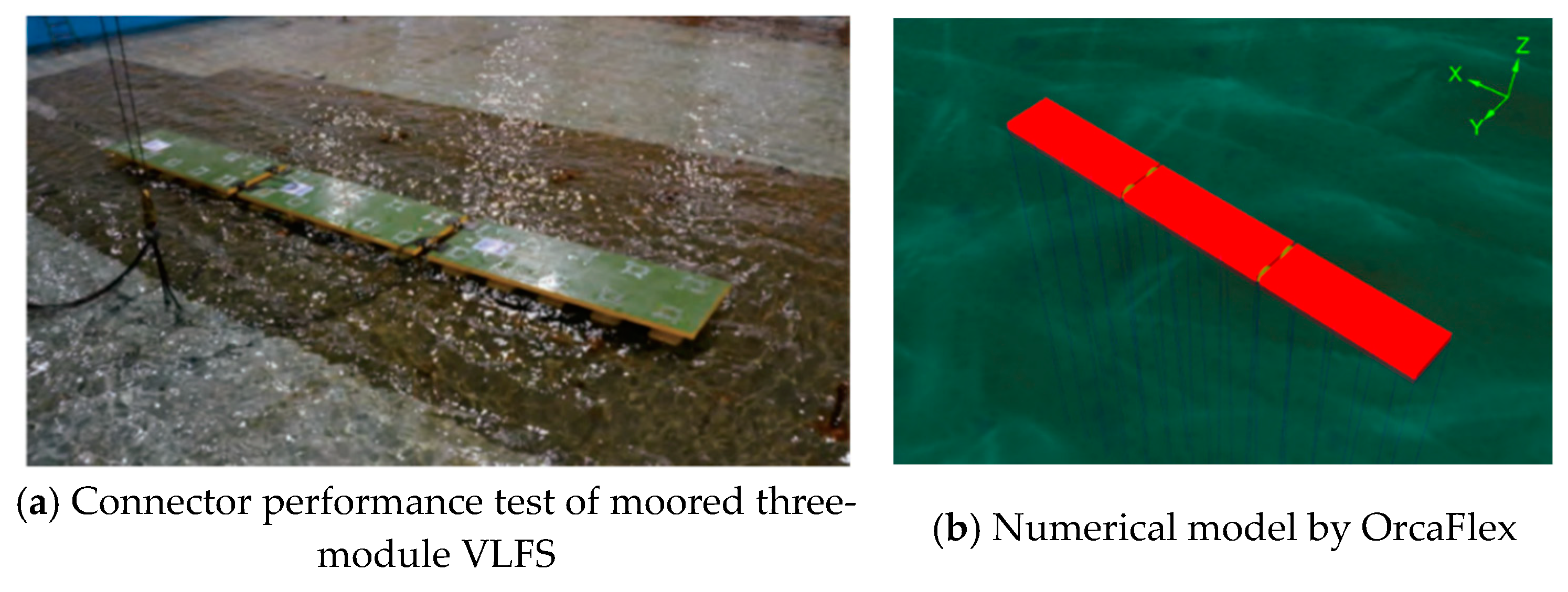
To validate the accuracy of the simulation method, a comparative analysis is carried out according to the experiments [40]. A series of experiments are performed to study the hydrodynamics of the very large floating structure, composed of three identical buoy modules, with a scale of 1:100, as shown in Figure 9a. One single buoy module is 3 m long, 1 m wide, and 0.27 m high and has a 0.12 m draught. The numerical model is shown in Figure 9b alongside the experimental model in Figure 9a.
Figure 9.
Experimental model [41] and numerical simplified model.
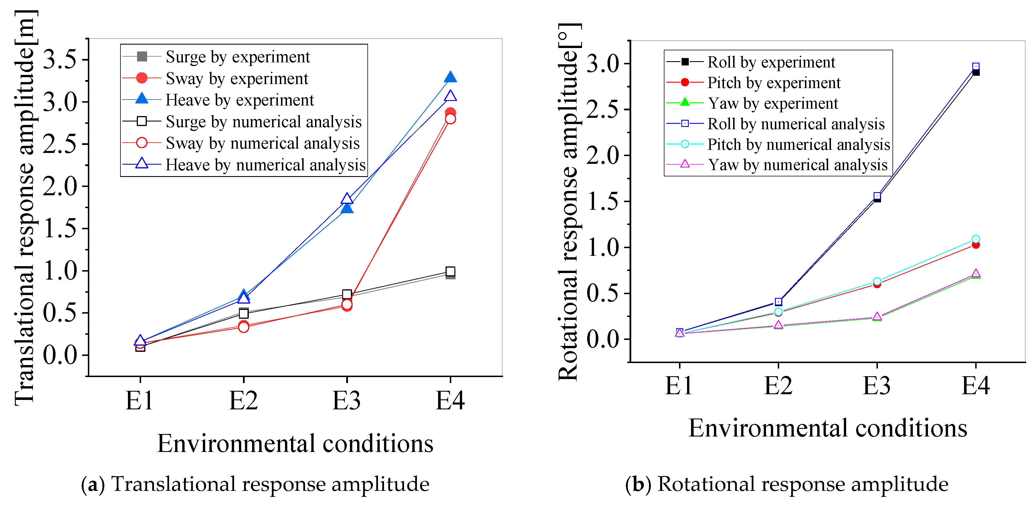
The amplitude of the motion response is half of the difference between the peak and trough of the response, by Equation (23).
The six-degree-of-freedom motion amplitudes of the intermediate buoy by numerical analysis are compared with the experimental results under the environmental conditions E1~E4, listed in Table 6. The maximum relative error between the numerical simulation and model experiment is 5.71% in sway by Equation (24), as shown in Figure 10.
Table 6.
Environmental conditions in experiments.
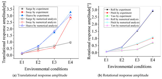
Figure 10.
The comparison between the experimental and simulation results.
4. Result Analysis
4.1. Buoy’s Motion and Acceleration
The FPV array comprises several buoys and many connectors between the buoys. The response of each buoy may be coupled with others, which cannot be simplified as a whole rigid body. As the wave first makes contact with the FPV array, the head buoys will oscillate severely as moorings fix the whole FPV. During the process of wave propagation, the FPV may oscillate as the wave crest is coupled with the connected buoys. It may also enlarge the motion of the buoys coupled with the adjacent ones. This paper investigates the motion and acceleration response of buoys under waves and currents and their combined action.
4.1.1. Wave-Induced Response
The buoy’s motion response increases with the wave height increase under different mooring tension levels, as shown in Figure 11. As the direction of the environmental load is 0 degrees, only the surge, heave, and pitch will be investigated, as other motions are not significantly affected.
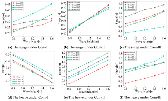
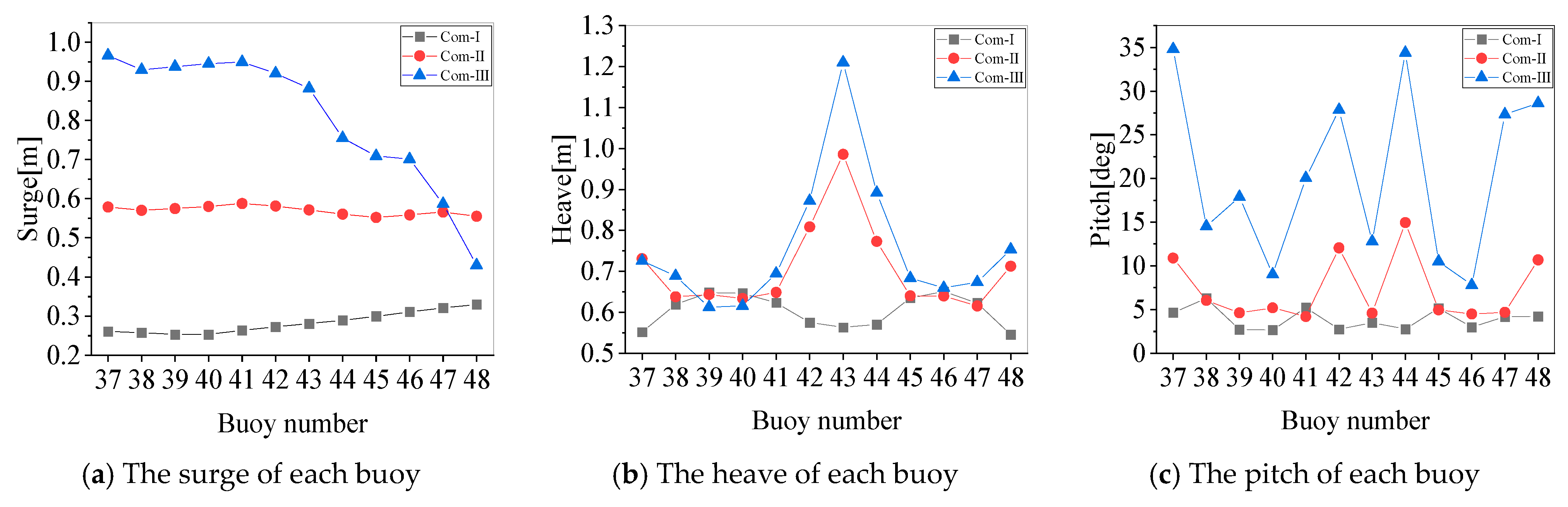
Figure 11.
The motion response of the buoys under different mooring tension levels with different wave heights.
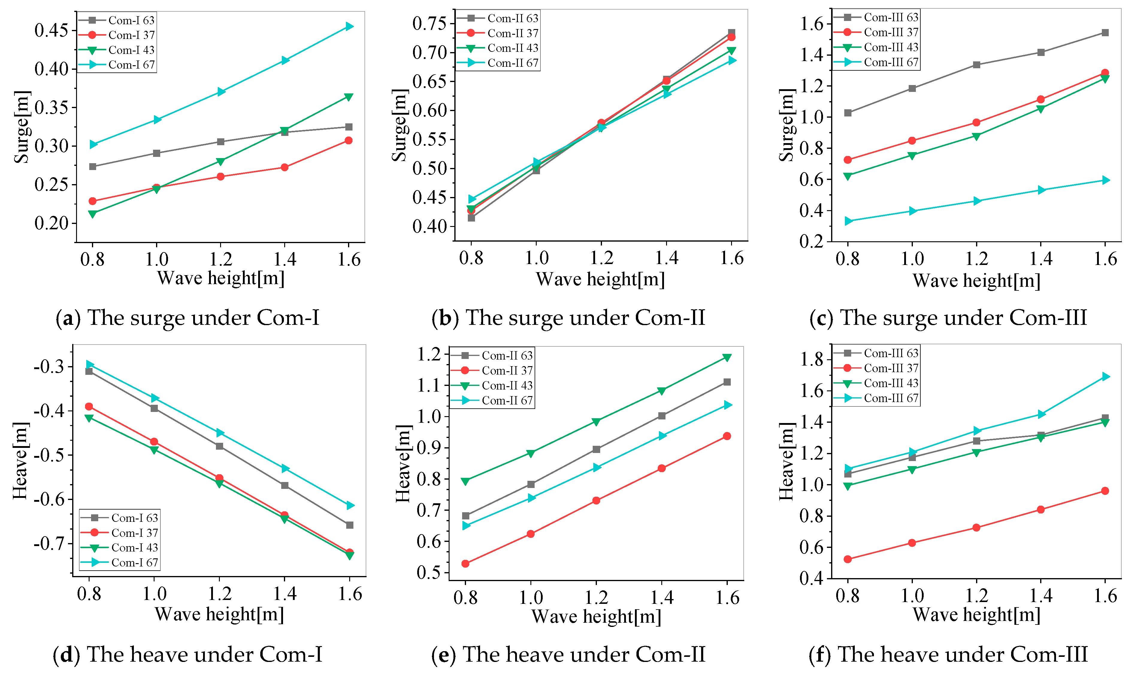
Under the mooring tension level Com-I, the surge response increases on the buoys along the direction of the wave propagation under waves with a 1.2 m height and 6 s period, but the reverse trend, that is the surge decreases along the wave direction when the mooring tension level decreases, is observed in Com-II and Com-III, as shown in Figure 12a. The wave height will increase the surge of the buoys and affect the largest or smallest response buoys distribution, as illustrated in Figure 11a–c. However, the surge of buoys 63 and 37 facing the wave, as shown in Figure 3, will increase slowly under Com-I, the smallest two under the 1.6 m wave height. Comparing the surge under different mooring tensions, the largest surge happens on buoy 67 facing away from the wave under Com-I, as shown in Figure 3, but the largest is on buoy 63 facing the waves under Com-III; the surge response of the buoys facing the wave exceeds 159.3% of the buoys facing away from the wave.
Figure 12.
The motion response of each buoy under different mooring tension levels with 1.2 m wave heights.
The heave motion response oscillates in a shape similar to the waves, as shown in Figure 12b. The largest response happens on buoys 39 and 46 in the middle of the offshore FPV array, as shown in Figure 3 under Com-I, while the largest is on the middle buoy 43 with more than a two times increase under Com-II and Com-III. As the large pitch of buoy 42 and buoy 44 is connected with buoy 43 along the wave direction, shown in Figure 12c, the heave of buoy 43 increases. With the increase in the wave height, the number of the buoys floating on the water surface increases as the wave passes through. There are 13 floating buoys in the array under Com-I with a wave height of 0.8 m. A total of 14 buoys distributed along the wave direction are immersed under the water surface as the wave crest passes and are exposed as the wave passes through. When the wave height increases to 1.0 m, all of them are exposed to the water surface.
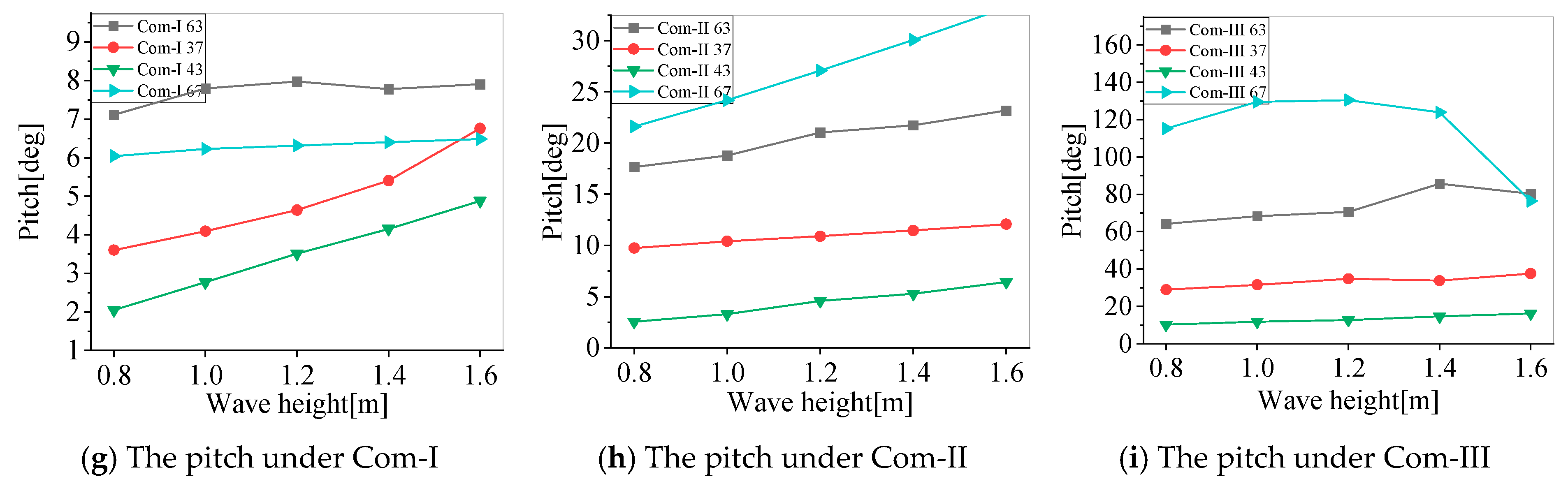
The severe fluctuations of the pitch on the buoys along the wave direction are given in Figure 12c. The decrease in the mooring tension level will increase the pitch significantly. The maximum pitch will occur on buoy 63, which is facing the wave under Com-I, but buoy 67 is facing away from the wave under Com-II and Com-III, as shown in Figure 12a–c.
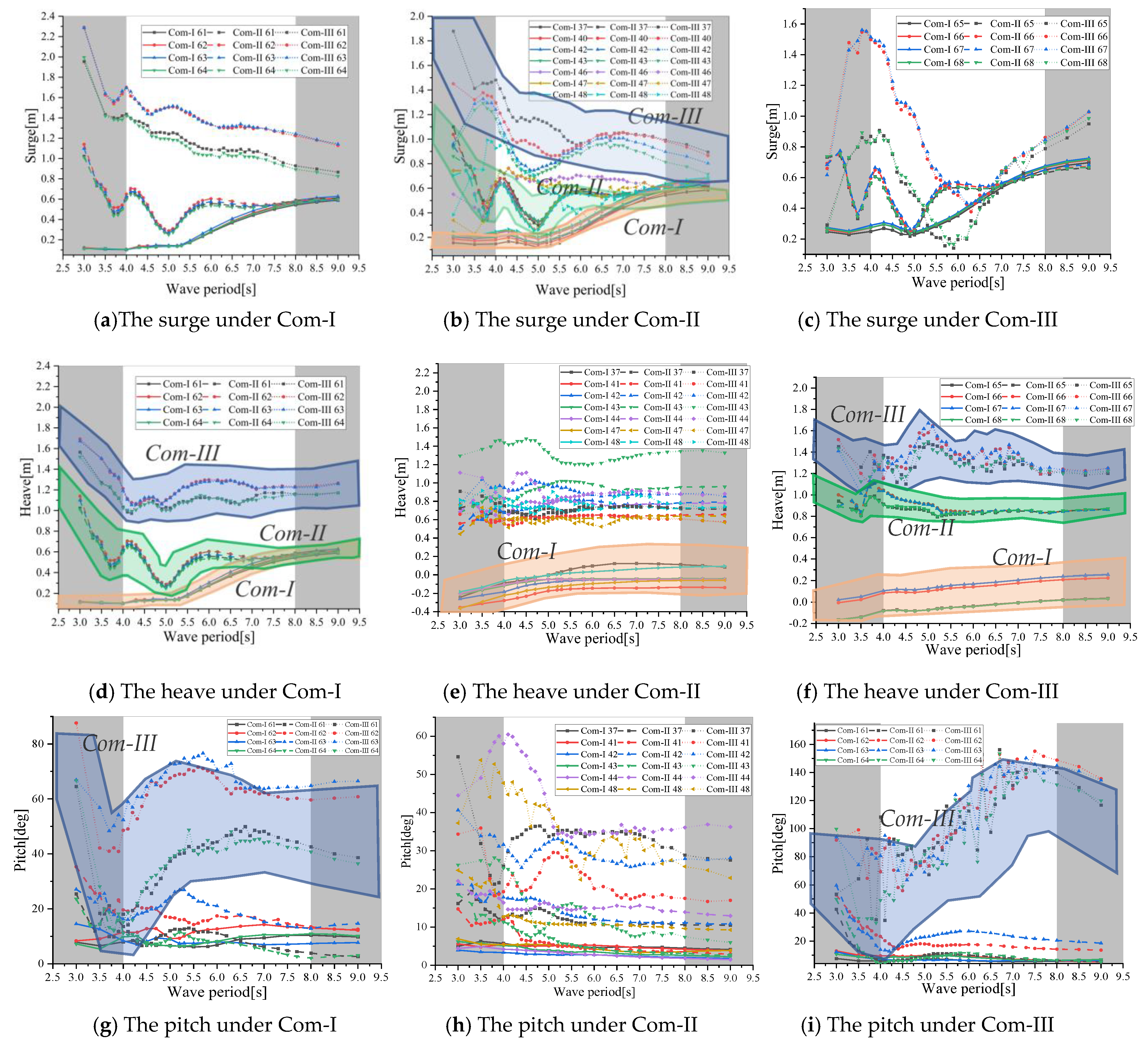
Keeping the wave height constant at 1.2 m, the effect of the wave period on the buoy motion response is investigated under different mooring tensions, as shown in Figure 13. The mooring tension level may have a significant influence on the buoy response. Under Com-I, the surge and heave will increase with the period, while the pitch will change slightly. Through the slight difference in the response of the different buoys, the buoys formed by the FPV may keep almost the same motions as the one floating platform under Com-I.
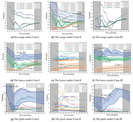
Figure 13.
The effect of the wave period on the surge motion response of the different buoys.
With the decrease in the constraint from the mooring, the surge response range will be significantly changed with the period in Com-II and Com-III. Comparing the surge under Com-I in Figure 13a, significantly different surges happen for the different buoys under Com-III, especially for the buoys facing away from the wave, based on the response in Figure 13a for the buoys facing the wave and in Figure 13c for the ones facing away from the wave. The effect transition of the wave as it passes through is shown in Figure 13b; for the middle buoys, the influence curve for buoy 37 is similar to the buoy facing the wave in Figure 13a, and the curve for buoy 48 is similar to the one facing away from the wave in Figure 13c. In one FPV array, different hydrodynamic characteristics occur for the different buoys, which adjacent buoys will couple. Under Com-II and Com-III, the heave and pitch response will fluctuate more severely than the response under Com-I, as shown in Figure 13d–i.
The buoys’ heave response changes with the wave period, influencing the immersion or exposure of the water station. Under Com-I, a large number of buoys are immersed by waves and are subjected to a wave period smaller than 4 s, but the number of immerged buoys decreases with the increase in the period, as shown in Figure 13d–f. Few buoys are immersed under Com-II and III.
Another significant factor is the mooring line position, which will have a great influence on the buoy stiffness under Com-III. Buoys 61 and 64 are linked with two mooring lines and are close to the corner mooring line, while buoys 62 and 63 are only linked with one mooring. With the relaxation of the mooring tension, the mooring conditions will affect the surge in Figure 13a, the heave in Figure 13a, and the pitch in Figure 13g—that is to say that more mooring lines will decrease the response significantly. A similar phenomenon also happens for buoys 65 and 68 and buoys 66 and 67, in Figure 13c,f,i. In contrast, the motion, including the surge, heave, and pitch, cannot be clearly separated for the different buoys with no mooring links, Figure 13b,e,h. It can be seen that the mooring condition will influence the buoy motion significantly for the multi-buoy FPV array. The effect of the wave period on the motion response of the different buoys is different.
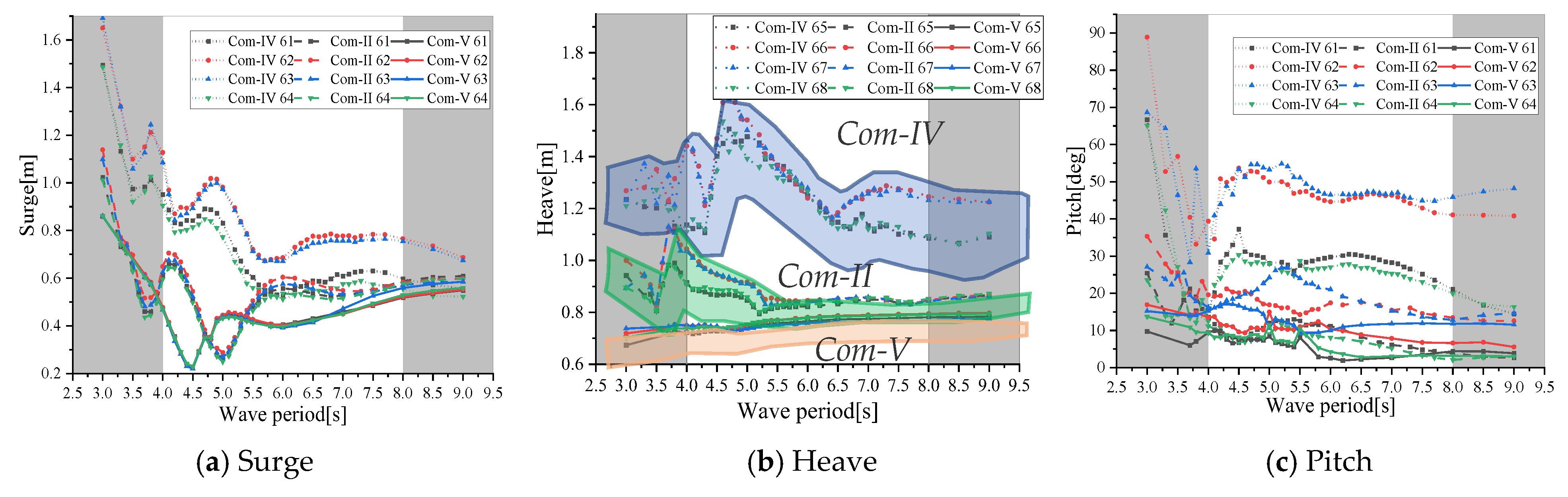
In order to reveal the characteristics and trends of the different mooring tension levels, Com-IV and Com-V are added with the same 29 m mooring length but with a 12 m and 18 m water depth, respectively. The surge, heave, and pitch results for different buoys are shown in Figure 14. The same trends have been illustrated for Com-I and Com-V, with high tension levels, as well as Com-III and Com-IV.
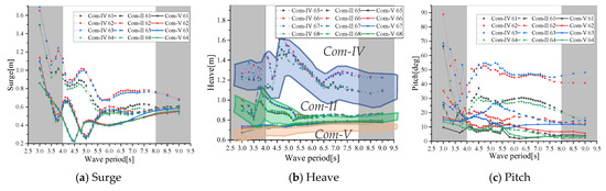
Figure 14.
The effect of the wave period on the motion response of the different buoys with a 29 m mooring length.
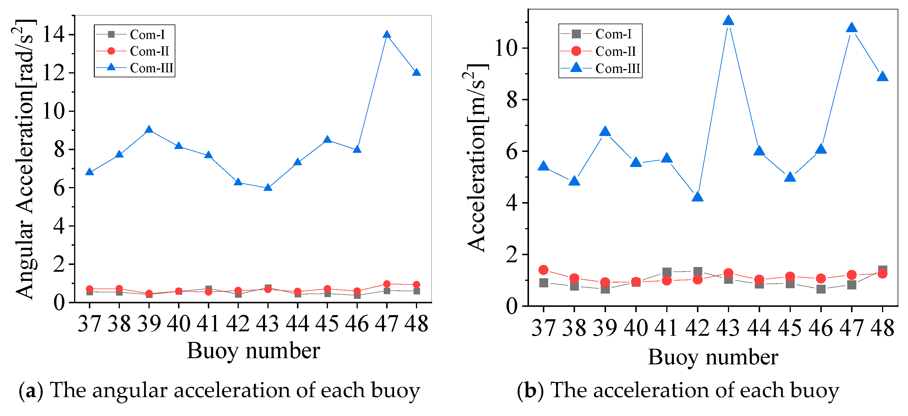
The accelerations, including resultant angular and displacement ones, are shown in Figure 15a,b, respectively, for the buoys along the direction of the wave propagation under the wave with a 1.2 m height and a 6 s period. Under Com-III, the angular acceleration increases sharply compared with the values under Com-I and Com-II and the displacement acceleration. It can be seen that the maximum angular acceleration happens to buoy 47 facing away from the wave, and the maximum acceleration occurs in Figure 15b to buoy 47 facing away from the wave and to the middle buoy 43. The displacement acceleration response of the buoy increases with the increase in the wave height, as shown in Figure 16. The acceleration of the buoys facing away from the wave is always greater than most other buoys in the array.
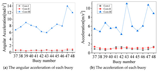
Figure 15.
The acceleration of the different buoys under different tension levels.
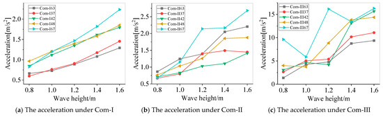
Figure 16.
The acceleration response of each buoy under different mooring tension levels with different wave heights.
The acceleration response of the buoys decreases with the change in the period and finally tends to be stable. With the relaxation of the mooring, the fluctuations increase severely. The acceleration response of the buoys facing away from the wave surface is larger than that of the ones facing the wave. At the same time, comparing the acceleration changes between the longitudinally arranged buoys, it can be seen that the acceleration response of the intermediate buoy 43 is larger than that of other buoys.
The buoys’ surge, heave, and pitch response in the FPV array is more intense under waves and increases with the wave height. The motion response of the buoys in different positions varied obviously. It can be seen that the tension level has a significant effect on the motion response of the buoy. As the effective tensions of the mooring lines were large, the differences in the motion response of the buoys were small. While the mooring lines were relaxed, the motion of the buoys significantly increased, and the motion response and acceleration response facing away from the wave surface were particularly severe.
4.1.2. Coupled Response of Buoys Under Wave–Current
Under the current load, the heave motion becomes large with the increase in the current velocity for the buoys facing the current under Com-I, in Figure 17b, with the same direction of the wave and current. It can be seen that as the current velocity increases, the buoys facing the current may increase in depth. The current will tighten the mooring line facing the current, with a similar effect of the enlargement of the mooring effect tension, but with a decrease in the mooring effect tension of the moorings facing away from the wave of the current. At the most tense mooring tension level, the array attitude is different from other tension levels. This will cause different trends combined with the wave–current and we compare the one under a wave or current only.
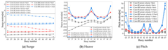
Figure 17.
Motion of buoys and tension of mooring line at different current velocities.
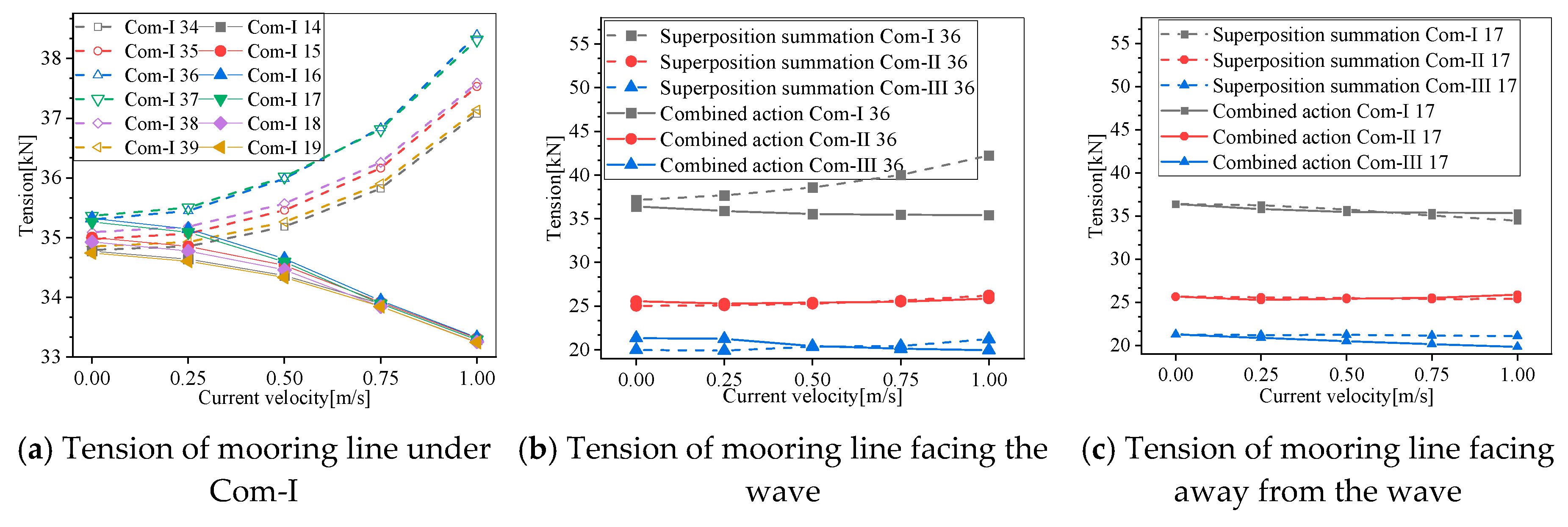
The response superposition summation and combined response for the buoy motions are illustrated in Figure 18 under an increasing current and the wave with a 1.2 m height and a 6 s period. As the current velocity increases, the surge motion increases under the combined wave and current. Obvious differences are illustrated for the response superposition summation and combined response in Figure 18a–c, especially for the buoys facing away from the wave under Com-III. The combined action of the waves and current suppresses the pitch motion response of the buoys, as shown in Figure 18d–f. The largest difference happens to the buoys under Com-III, and a slight difference is obtained for the heave.
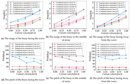
Figure 18.
Superposition summation and combined response of buoy motions with increasing current.
Figure 19 shows the motion response under increasing wave heights and a current of 0.5 m/s compared to the superposition summation. With the increased wave height, the surge increases significantly, and obvious differences occur between the superposition summation and combined response in Figure 19a–c. Similar trends occur in the pitch response, as shown in Figure 19d–f. But small differences occur to the heave.
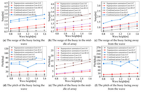
Figure 19.
Superposition summation and combined response of buoy motions with increasing wave height.
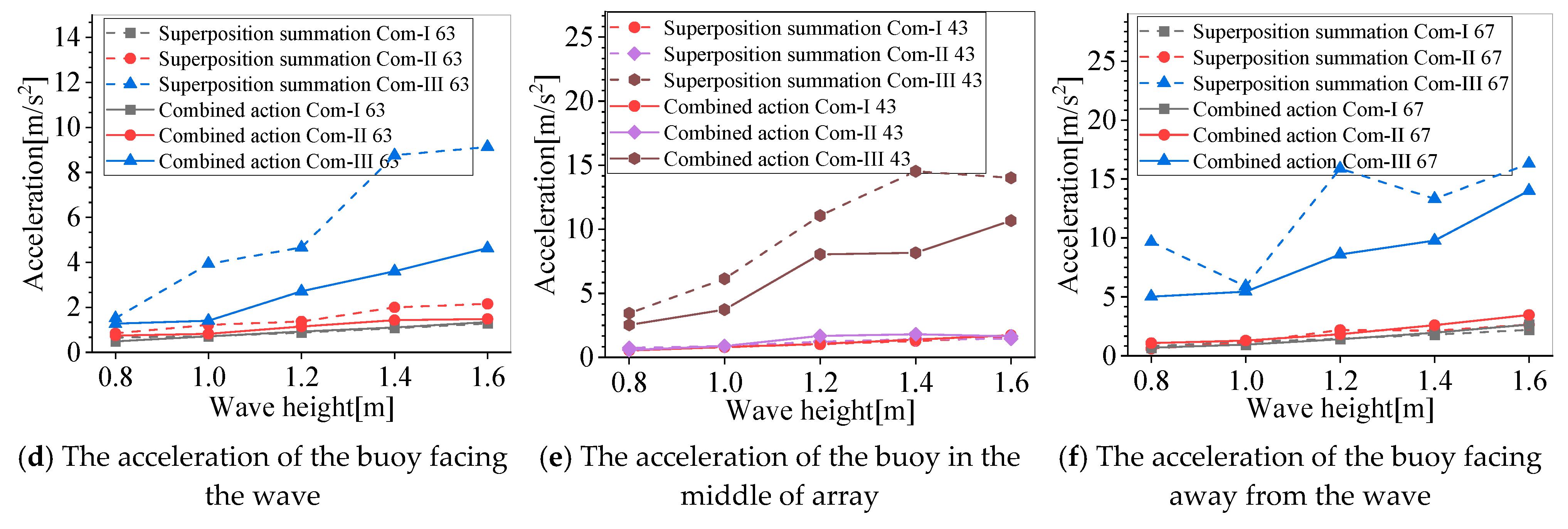
Under the current only, the acceleration of the buoy is small as it reaches a steady state. The results of the superposition summation are quite different from those of the combined wave–current action, as shown in Figure 20. The superposition summation acceleration is larger than the combined results, especially under Com-III. It can be seen that the current will restrain the acceleration response of the buoy. This constraint effect is different under different waves or currents. This phenomenon Is most evident under Com-III.
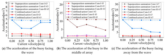
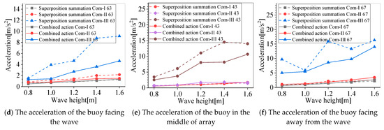
Figure 20.
Acceleration of buoy in superposition summation and combined action.
The surge motion of the buoys increased in the combined action, while the motions in other directions decreased, and the acceleration of the buoys also decreased. The current changed the tension of the mooring lines in the FPV array. When the mooring lines were relaxed, the motion amplitude of the array increased. When the current increased the tension of the mooring lines, the FPV array was tilted forward as a whole. The buoys in front of the array were immersed and the mooring connected to it was completely tensed, while the buoys on the surface facing away from the wave were weakened by the mooring constraint with the violent motion.
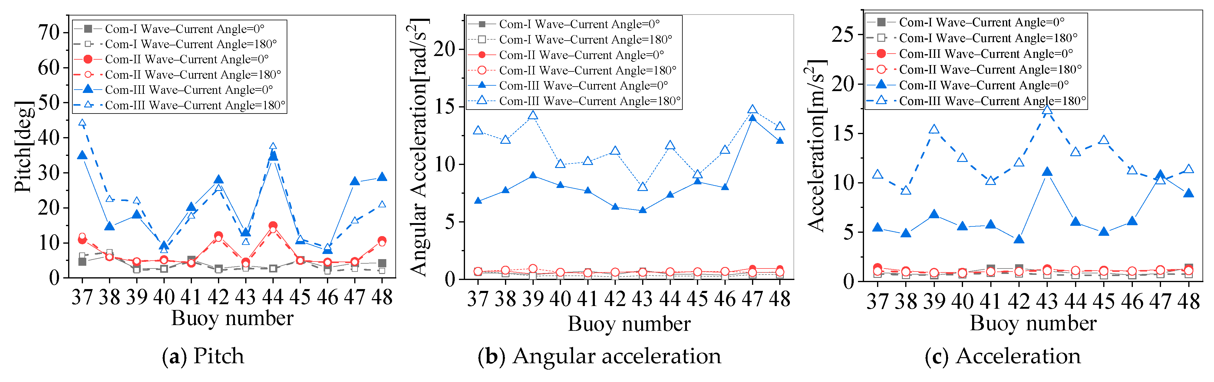
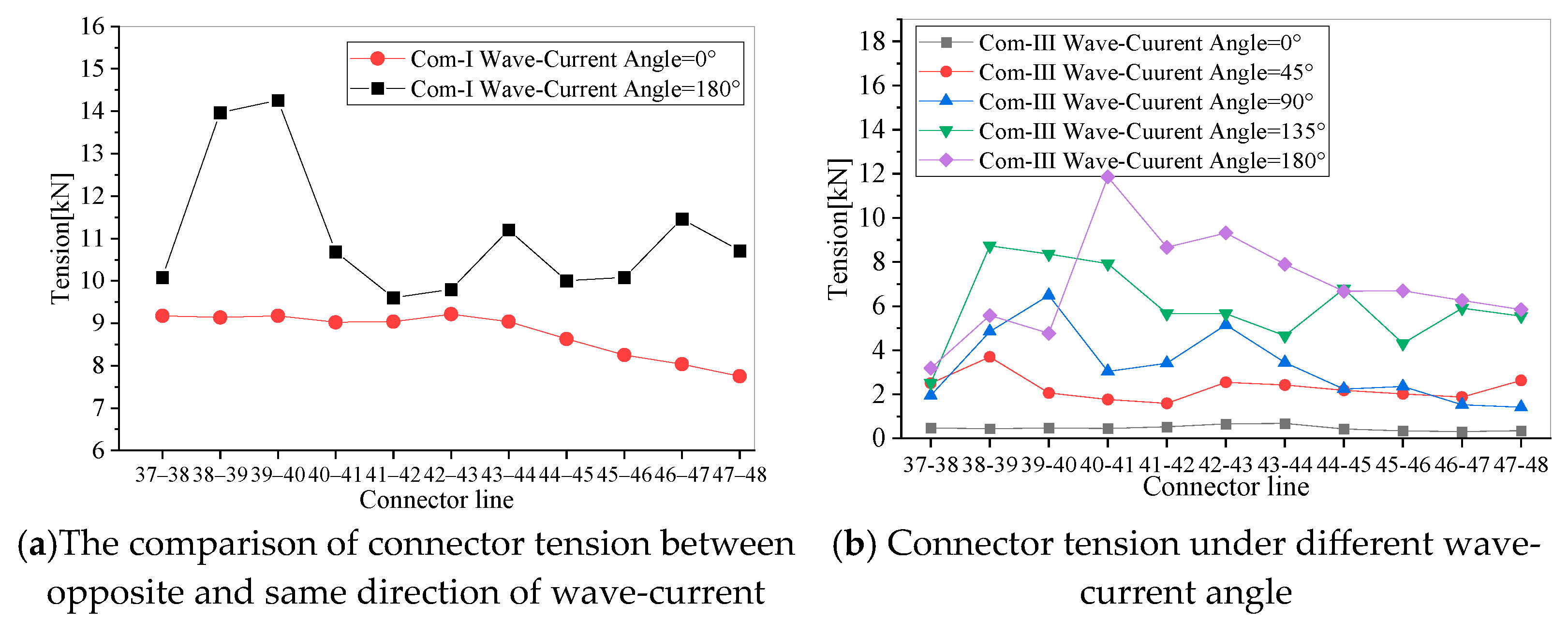
As the wave–current move in the opposite direction, the wave–current angle is 180°, and the current will tighten the moorings facing away from the wave and relax the moorings facing the wave. The comparisons are shown in Figure 21. The pitch of buoy 37 facing the wave will increase significantly as the wave and current move in the opposite direction (wave–current angle = 180°), Figure 21a, as will the acceleration in Figure 21b,c.
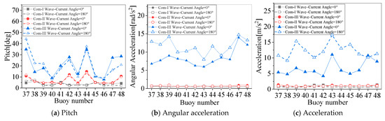
Figure 21.
The motion response of each buoy under different mooring tension levels with the wave–current in the same and opposite direction.
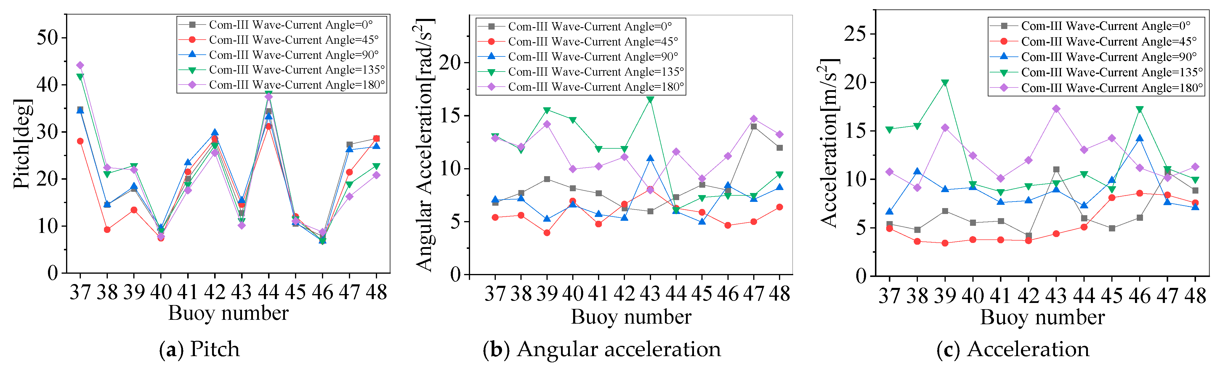
The response of the buoys in different wave–current angles in Com-III affects the mooring tension levels, as shown in Figure 22. With the increase in the wave–current angle, the current will relax the moorings facing the wave and tighten the moorings facing away from the wave. When the wave–current angle is greater than 90°, the pitch motion response of the buoys facing the wave increases and the motion response of the buoys facing away from the wave increases, as shown in Figure 22a; the pitch response of the buoy facing the wave is increased by 9.36°, and the acceleration in Figure 22b,c is also increased. The acceleration of buoy 37 facing the wave increased by 5.39 m/s2, and the acceleration of buoy 48 facing away from the wave increased by 2.45 m/s2. And the angular acceleration of the buoys is increased, e.g., the acceleration of buoy 39 is increased by 348.2%.
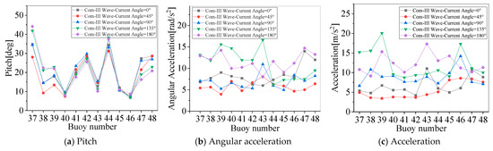
Figure 22.
The response of each buoy under Com-III mooring tension levels with different wave–current angles.
4.2. Coupled Mooring Tension
Waves are the primary loads for the offshore FPV, which differs from the situation inland or in lakes. As the moorings are set on different buoys linked with its adjacent buoys, the tension may be influenced by the interaction of the buoys under waves. The wave effect will be studied to investigate the characteristics of the mooring tension at the frontal wave surface and the facing away from the wave surface of the FPV array.
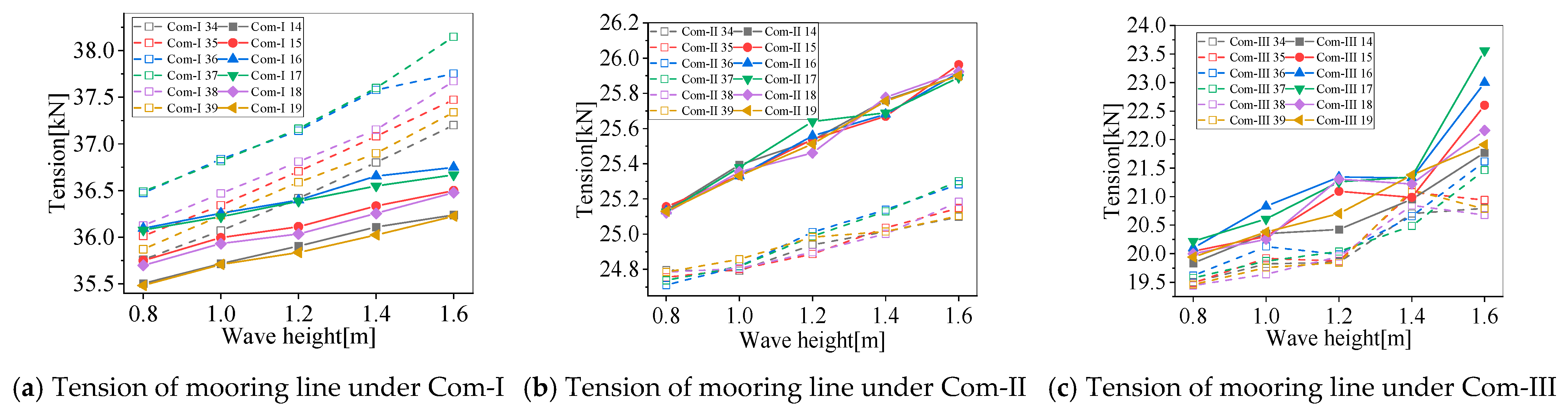
Due to the mooring lines located on different buoys in the multi-buoy FPV array, this paper may have some uncommon results compared to the single buoy platform. As shown in Figure 23, the mooring tension increases with the wave height. The maximum mooring tension happens in the array under Com-I in Figure 23a. However, the tension for the moorings facing away from the wave are larger than the ones facing the wave under Com-II in Figure 23b and Com-III in Figure 23c, due to the severe motion of the buoy facing away from the wave.
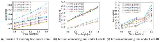
Figure 23.
Tension of mooring line at different tension levels under different wave heights.
The mooring line tension changes with the wave period, as shown in Figure 24. In the range of this study, a trend of fluctuation decreasing towards stability with the change in the wave period is provided for the mooring line tension, and more fluctuations are present in Com-III. Under Com-III, the tension of the moorings facing away from the wave are larger than the ones facing the wave.
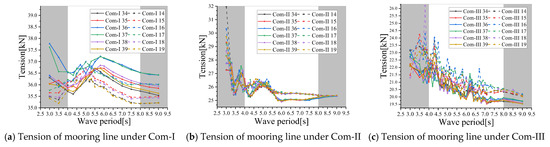
Figure 24.
Tension of mooring line at different tension levels under different wave periods.
The current load only changes the position of the FPV array and increases the mooring tension. The increase in the current increases the tension of the moorings facing the current but decreases the tension of the moorings against the current, as shown in Figure 25a. It will change the binding force of the moorings on the FPV array. Therefore, the results of the mooring tension are different between the superposition and combined action, as shown in Figure 25b,c. Under the combined wave–current, the tension of the mooring facing the wave decreases with the increase in the current, but increases with the increase in the current for buoys facing away from the wave. It can be seen that under the combined wave and current, the opposite tension change trend is illustrated for the moorings facing the wave and the ones facing away from the wave. The difference between the superposition and combined action is the largest for the tension of the moorings facing the wave under Com-I, in Figure 25b.
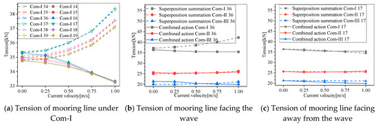
Figure 25.
Mooring line at Com-I under different current velocities and difference between superposition summation and combined action of tension of moorings.
The mooring tension increased with the waves but varied in different positions. With a large effective tension, the tension of the mooring line facing the wave was larger than that facing away from the wave. With the relaxation of the mooring, the maximum tension of mooring lines facing away from the wave was larger than those facing the wave. This is due to the offset of the array; the constraint of the moorings facing away from the wave on the buoys was weakened, resulting in the violent motion of the buoys. The maximum tension of the mooring facing away from the wave decreased as the current velocity increased. The tension of the mooring in the combined action of the wave and current was smaller than the superposition.
4.3. Connector Tension
As the wave crest passes through the FPV, the surge of the buoys may increase greatly, while the connector force may also increase significantly. Another important factor is each buoy’s motion and connector force distribution along the wave, which is the maximum value position.
4.3.1. The Effect of Waves on the Longitudinal Connectors’ Tension
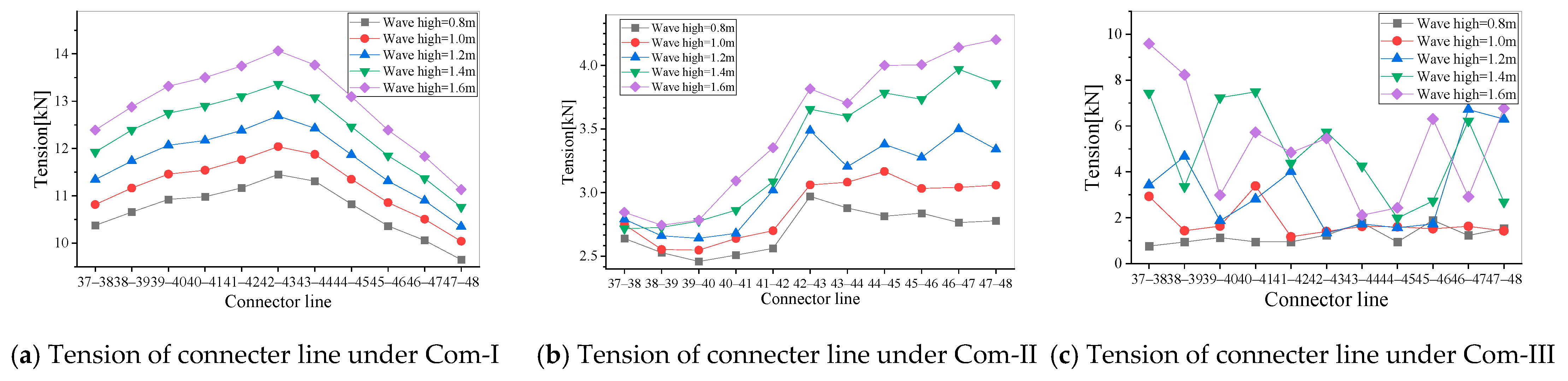
The trend curves of the connector tension with the wave height are shown in Figure 26a under Com-I, Com-II, and Com-III. The connector tension increases linearly with the wave height under Com-I and Com-II. More fluctuations and rapid increases will happen for the connector tension under Com-III due to the buoys’ severe motion resulting from the mooring’s relaxation. With the increase in the mooring static tension level, the tension of the connectors between the buoys increases as the wave height is less than 1.0 m. However, the maximum connector tension is obtained under Com-I.
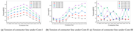
Figure 26.
Tension of connector line at different tension levels under different wave heights.
To illustrate the connector tension for different buoys, a series of results for the connector along the wave propagation are given in Figure 26a–c for Com-I, Com-II, and Com-III, respectively. Under the high mooring static tension in Com-I, the connector tension increases with the wave propagation but decreases as the wave passes through buoy 43, the middle aisle buoy. So, the tension of the connectors between buoy 42 and 43 is the largest. Under Com-II, the tension increases for the buoys, similarly to Com-I, but as the wave passes through buoy 43, the tension maintains a large value under the wave height less than 1.2 m and increases under large wave heights. The maximum tension happens for the buoy facing away from the wave. Under Com-III, for a wave height less than 1.0, the connectors for the buoys along the wave propagation maintain a small value. But under a large wave height, the connector tension increases sharply with the increase in the wave height, as the maximum value occurs in the buoy near the position facing the wave and facing away from the wave.
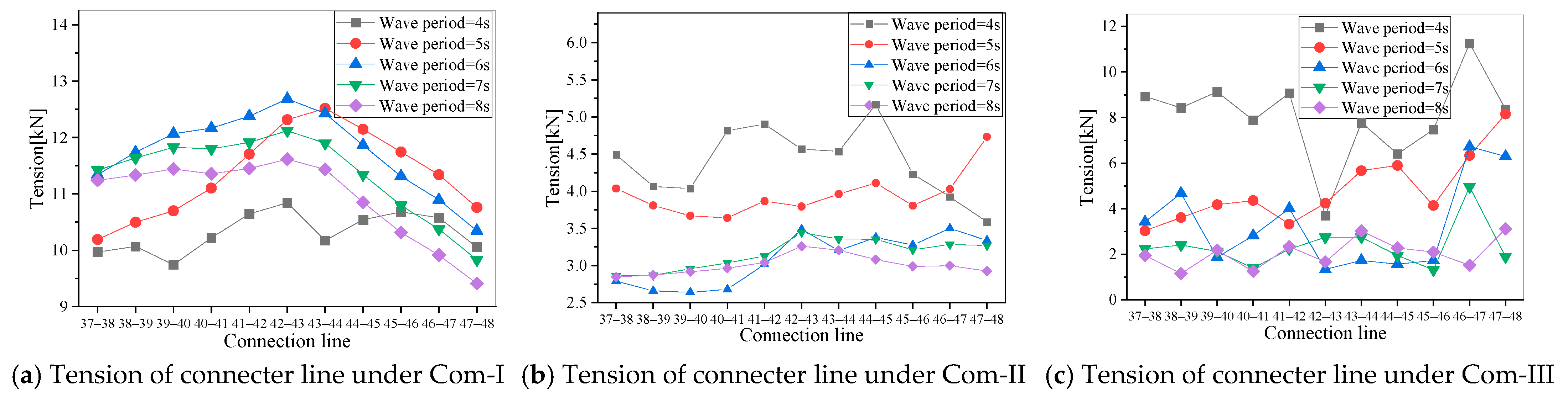
The connector tension decreases with the wave period. Under the different mooring static tensions, a similar trend of the connector tension with the wave period is shown with the tension changed with the wave height in Figure 27a–c for Com-I, Com-II, and Com-III, respectively. The maximum value happens under the wave with a small period due to the small size of the buoys. Under the wave with a large period, the tension range is smaller than the value under the small period wave.
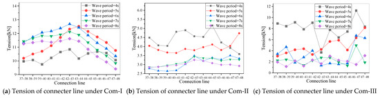
Figure 27.
Tension of connection line at different tension levels under different wave periods.
The current load only changes the array position and increases the mooring tension, as shown in Figure 27. However, the heave motion becomes large with the increase in the current velocity for the buoys facing the current under Com-I, in Figure 27b. It can be seen that as the current velocity increases, the buoys facing the current may increase in depth. The increase in the current increases the tension of the moorings facing the current but decreases the tension of the moorings against the current, as shown in Figure 27c.
When the mooring tension level is high, the tension of the internal connectors in the array along the wave direction varied obviously. The maximum connector tension happened in the middle of the array. With the relaxation of the moorings, the tension of the connectors increased rapidly with the wave height. The maximum tension of the connectors happened near the buoys facing the wave and facing away from the wave under the mooring tension in Com-III.
4.3.2. Coupled Effect
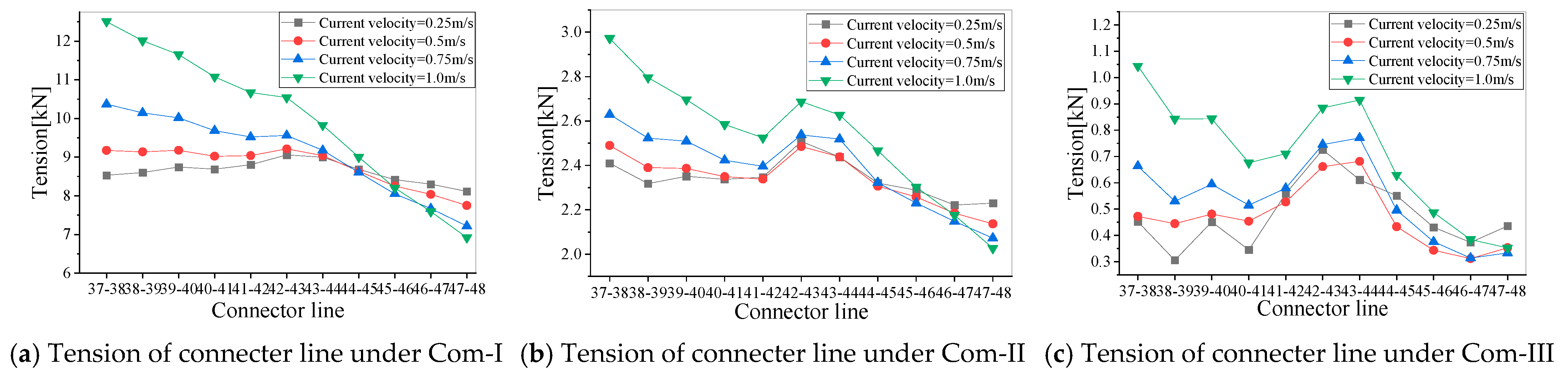
In the same direction of the wave and current, with the increase in the mooring tension level, the tension of the connectors increases, as shown in Figure 28. Figure 28a–c represent the tension changes in connectors between the longitudinal buoys under three different tension levels. When the mooring is in the most tense state, the tension of the connectors between the longitudinal buoys is quite different, and the tension of the connectors near the surface facing away from the wave, which is between buoy 47 and 48, even decreases with the increase in the current velocity, as shown in Figure 28a.

Figure 28.
Tension of connector line at different tension levels under different current velocities.
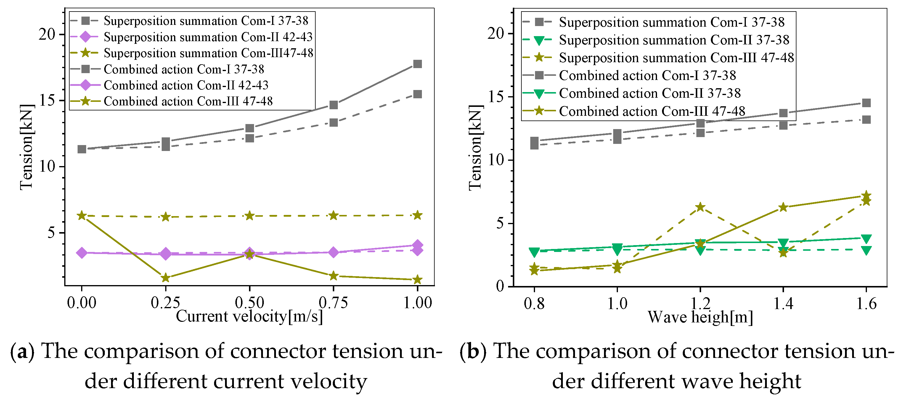
Figure 29 shows that the differences between the superposition summation and combined action are also obvious for the mooring tensions. Under Com-I, the combined action result is larger than the superposition. Meanwhile, under Com-III, the trend is the opposite, and the combined result is less than the superposition one.
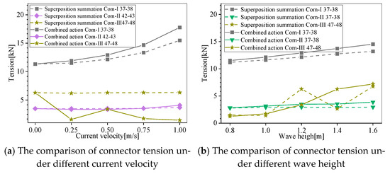
Figure 29.
Connector tension in superposition summation and combined action.
Under the wave–current in the opposite direction, the wave–current angle is 180°, and the current will relax the moorings facing the wave. It will result in the sharp increase in the connection force of the buoys facing the wave, as shown in Figure 30. Under the most relaxed mooring tension level in Com-III, in Figure 30b, the relaxation increases with the increase in the wave–current angle, and the connector cannot be effectively tensed when the wave–current is in opposite direction, the constraint is weak, and the relative motion between the buoys is intense. The maximum tension of the connector under the wave is larger than that under the wave–current in same direction, by 11.4 kN.
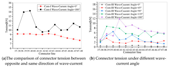
Figure 30.
Tension of connector line at different tension levels under different wave–current angles.
5. Conclusions
The multi-buoy FPV array under the effect of waves and currents is investigated using a numerical method. The buoy motion response, acceleration, connector tension, and mooring tension of the offshore FPV under different mooring tensions are studied as the array under waves only and under a combined wave and current action. The conclusions are as follows:
- (1)
- When responding only to wave excitation, the motion response, including the surge, heave, and pitch, of the buoys in the FPV oscillates severely and increases with the wave height. The effects of the mooring static tension on the hydrodynamic characteristics are obvious for the multiple buoys connected to each other, especially for the buoys facing away from the wave. The maximum mooring tension occurs on moorings facing the wave, as in the array under Com-I. Under Com-III, the tension of the moorings behind the wave is larger than the ones facing the wave. This is the difference between different mooring tensions, which causes the difference in the response of the buoys facing away from the wave under different mooring tensions.
- (2)
- The coupled effect of the wave–current is significant for the floating multi-buoy array. Under the combination action, the motions and accelerations of the buoys facing the actions are decreased as the moorings facing the wave and current are tightened, as the wave and current are in the same direction. Meanwhile, the motions of the buoys facing away from the wave will be violent as they are relaxed.
- (3)
- With the increase in the wave–current angle, the constrained effect of the current on the moorings and connectors is weakened. This results in the increase in the motions, acceleration, and connection force of the buoys facing away from the current and facing the wave, as the pitch response increased by 9.36°, the acceleration by 5.39 m/s2, and the connection by 11.40 kN under the wave and current in the opposite direction (wave–current angle = 180°).
In this research, the combined effect of waves and currents has a great influence on the response of the flexible multi-buoy FPV array. A series of detailed studies on this phenomenon will be conducted in future research, including the influence of a non-uniform current, the response under viscous fluids, and the experiment verification.
Author Contributions
Conceptualization, X.-H.S., J.Z., C.G.S., J.Y. and H.L.; methodology, X.-H.S. and J.Z.; software, Y.W. and J.Z.; validation, X.-H.S., Y.W., J.Y. and H.L.; formal analysis, X.-H.S., Y.W., J.Y. and H.L.; investigation, Y.W. and H.L.; resources, J.Y. and H.L.; data curation, Y.W.; writing—X.-H.S. and Y.W.; writing—review and editing, J.Z. and C.G.S.; visualization, Y.W., J.Y. and H.L.; supervision, J.Z. and C.G.S.; project administration, J.Y. and H.L.; funding acquisition, J.Y. and H.L. All authors have read and agreed to the published version of the manuscript.
Funding
This research was funded by Huadian Heavy Industry Co., Ltd. (HHI-KJ-2022-22), “Research on the decision system and safety of the installation for the offshore wind turbine”, and the Key Research and Development Program for Core Technology by the Nantong City government (JB2024009), “Key technology and industrialization for installation of high-power wind turbine foundations in far deep Sea efficiently”.
Data Availability Statement
Data are contained within the article.
Conflicts of Interest
Author Honglong Li was employed by the company Zhongtian Technology Marine Engineering Co., Ltd., author Jia Yu was employed by the company Huadian Heavy Industries Co., Ltd. The remaining authors declare that the research was conducted in the absence of any commercial or financial relationships that could be construed as a potential conflict of interest.
References
- Baolei, G.; Xu, T.; Ruijia, J.I. Research prospects for offshore floating photovoltaic structures and their hydrodynamic problems. Ocean. Eng. 2024, 42, 190–208. [Google Scholar] [CrossRef]
- Temiz, M.; Dincer, I. Techno-economic analysis of green hydrogen ferries with a floating photovoltaic based marine fueling station. Energy Convers. Manag. 2021, 247, 114760. [Google Scholar] [CrossRef]
- Golroodbari, S.Z.M.; Vaartjes, D.F.; Meit, J.B.L.; van Hoeken, A.P.; Eberveld, M.; Jonker, H.; van Sark, W.G.J.H.M. Pooling the cable: A techno-economic feasibility study of integrating offshore floating photovoltaic solar technology within an offshore wind park. Sol. Energy 2021, 219, 65–74. [Google Scholar] [CrossRef]
- Ocean of Energy. A World’s First: Offshore Floating Solar Farm Installed at the Dutch North Sea. 2019. Available online: https://oceansofenergy.blue/ (accessed on 15 March 2025).
- Onsrud, M. An Experimental Study on the Wave-Induced Vertical Response of an Articulated Multi-Module Floating Solar Island. Master’s Thesis, Norwegian University of Science and Technology, Trondheim, Norway, 2019. [Google Scholar]
- Ocean Sun. Gallery | Ocean Sun. Available online: https://oceansun.no/gallery/ (accessed on 12 March 2025).
- Lee, G.Y.; Joo, H.J.; Yoon, S.J. Design and installation of floating type photovoltaic energy generation system using FRP members. Sol. Energy 2014, 108, 13–27. [Google Scholar] [CrossRef]
- Offshore Energy. SolarDuck Taking Floating Solar Further Offshore. 2021. Available online: https://www.offshore-energy.biz/solarduck-taking-floating-solar-further-offshore/ (accessed on 15 March 2025).
- CIMC. The First Semi-Submersible Offshore Photovoltaic Power Generation Platform in China Was Delivered By Cimc Raffles. 2023. Available online: https://www.offshore-mag.com/renewable-energy/article/14292287/cimc-raffles-delivers-chinas-first-semisub-floating-solar-power-platform (accessed on 7 March 2025).
- Newman, J.N. Wave effects on deformable bodies. Appl. Ocean. Res. 1994, 16, 47–59. [Google Scholar] [CrossRef]
- Hong, S.Y.; Kim, J.H.; Cho, S.K.; Choi, Y.R.; Kim, Y.S. Numerical and experimental study on hydrodynamic interaction of side-by-side moored multiple vessels. Ocean Eng. 2005, 32, 783–801. [Google Scholar] [CrossRef]
- Lee, C.H.; Newman, J.N. An assessment of hydroelasticity for very large hinged vessels. J. Fluids Struct. 2000, 14, 957–970. [Google Scholar] [CrossRef]
- Tajali, Z.; Shafieefar, M. Hydrodynamic analysis of multi-body floating piers under wave action. Ocean Eng. 2011, 38, 1925–1933. [Google Scholar] [CrossRef]
- Qian, J.; Sun, L.; Song, L. Material selection for hawsers for a side-by-side offloading system. J. Mar. Sci. Appl. 2014, 13, 449–454. [Google Scholar] [CrossRef]
- Pessoa, J.; Fonseca, N. Guedes Soares. Side-by-side FLNG and shuttle tanker linear and second order low frequency wave induced dynamics. Ocean Eng. 2016, 111, 234–253. [Google Scholar] [CrossRef]
- Bispo, I.B.S.; Mohapatra, S.C.; Soares, C.G. Numerical analysis of a moored very large floating structure composed by a set of hinged plates. Ocean Eng. 2022, 253, 110785. [Google Scholar] [CrossRef]
- Ding, J.; Wu, Y.-S.; Zhou, Y.; Ma, X.-Z.; Ling, H.J.; Xie, Z. Investigation of connector loads of a 3-module VLFS using experimental and numerical methods. Ocean Eng. 2020, 195, 106684. [Google Scholar] [CrossRef]
- Xu, S.; Wang, S.; Soares, C.G. Review of mooring design for floating wave energy converters. Renew. Sustain. Energy Rev. 2019, 111, 595–621. [Google Scholar] [CrossRef]
- Marco, R.-C.; Tina, G.M. Floating PV Plants; Academic Press: New York, NY, USA, 2020. [Google Scholar]
- Ormberg, H.; Larsen, K. Coupled analysis of floater motion and mooring dynamics for a turret-moored ship. Appl. Ocean. Res. 1998, 20, 55–67. [Google Scholar] [CrossRef]
- Kim, Y.S.; Choi, E.; Yoon, S.J.; Lee, S.O. Three dimensional hydrodynamic-structural analysis of floating type photovoltaic composite structure. In Proceedings of the Advances in Interaction & Multiscale Mechanics (AIMM’10), Jeju, Republic of Korea, 30 May 2010. [Google Scholar]
- Trapani, K.; Millar, D. Hydrodynamic Overview of Flexible Floating Thin Film PV Arrays. In Proceedings of the 3rd Offshore Energy and Storage Symposium, Valletta, Malta, 13–15 July 2016. [Google Scholar]
- Borvik, P.P. Experimental and Numerical Investigation of Floating Solar Islands. Master’s Thesis, NTNU, Taiwan, China, 2017. [Google Scholar]
- Winsvold, J. An Experimental Study on the Wave-Induced Hydroelastic Response of a Floating Solar Island. Master’s Thesis, NTNU, Taiwan, China, 2018. [Google Scholar]
- Kong, Y. Mooring Research of New-Type Floating Structure. Master’s Thesis, Shanghai Jiao Tong University, Shanghai, China, 2019. [Google Scholar]
- Liang, M.; Xu, S.; Wang, X.; Ding, A. Simplification of mooring line number for model testing based on equivalent of vessel/mooring coupled dynamics. J. Mar. Sci. Technol. 2020, 25, 573–588. [Google Scholar] [CrossRef]
- Liang, M.; Xu, S.; Wang, X.; Ding, A. Experimental evaluation of a mooring system simplification methodology for reducing mooring lines in a VLFS model testing at a moderate water depth. Ocean Eng. 2021, 219, 107912. [Google Scholar] [CrossRef]
- Sree, D.K.; Law, A.W.-K.; Pang, D.S.C.; Tan, S.T.; Wang, C.L.; Kew, J.H.; Seow, W.K.; Lim, V.H. Fluid-structural analysis of modular floating solar farms under wave motion. Sol. Energy 2022, 233, 161–181. [Google Scholar] [CrossRef]
- Mohapatra, S.C.; Soares, G.C.; Belibassakis, K. Current Loads on a Horizontal Floating Flexible Membrane in a 3D Channel. J. Mar. Sci. Eng. 2024, 12, 1583. [Google Scholar] [CrossRef]
- Clemente, G.; Ramos-Marin, S.; Soares, G.C. Advances in Maritime Technology and Engineering; Taylor & Francis: London, UK, 2024; pp. 417–425. [Google Scholar]
- Faltinsen, O.M. Sea Loads on Ships and Offshore Structures; Cambridge university press: Cambridge, UK, 1993. [Google Scholar]
- Tcheou, G. Non-Linear Dynamics of Mooring Lines. Doctor’s Thesis, Massachusetts Institute of Technology Department of Ocean Engineering, Cambridge, MA, USA, 1997. [Google Scholar]
- Karadeniz, H.; Saka, M.P.; Togan, V. Water Wave Theories and Wave Loads. In Stochastic Analysis of Offshore Steel Structures: An Analytical Appraisal; Karadeniz, H., Ed.; Springer: London, UK, 2013; pp. 177–252. [Google Scholar]
- Fenton, J.D. A Fifth-Order Stokes Theory for Steady Waves. J. Waterw. Port Coast. Ocean. Eng. 1985, 111, 216–234. [Google Scholar] [CrossRef]
- Young, I.R. Chapter 2—Wave Theory. In Elsevier Ocean Engineering Series; Young, I.R., Ed.; Elsevier: New York, NY, USA, 1999; pp. 3–23. [Google Scholar]
- Brevik, I.; Bjørn, A. Flume experiment on waves and currents. I. Rippled bed. Coast. Eng. 1979, 3, 149–177. [Google Scholar] [CrossRef]
- Morison, J.R.; Johnson, J.W.; Schaaf, S.A. The Force Exerted by Surface Waves on Piles. J. Pet. Technol. 1950, 2, 149–154. [Google Scholar] [CrossRef]
- Orcina. Orca Flex User Manual, Version 11.0; Orcina: Cumbria, UK, 2011.
- Yang, Y.; Bashir, M.; Li, C.; Wang, J. Investigation on Mooring Breakage Effects of a 5 MW Barge-Type Floating Offshore Wind Turbine Using F2A. Ocean Eng. 2021, 233, 108887. [Google Scholar] [CrossRef]
- Wang, Y.; Wang, X.; Xu, S.; Ding, A. Effects of stiffness parameters of flexible connectors of multi-module very large floating structure. Pet. Eng. Constr. 2020, 46, 145–151. [Google Scholar]
- Wang, Y.; Wang, X.; Xu, S.; Ding, A. Influence of multi-module VLFS connector stiffness on dynamic response performance. Ocean Eng. 2018, 36, 11–18. [Google Scholar]


Disclaimer/Publisher’s Note: The statements, opinions and data contained in all publications are solely those of the individual author(s) and contributor(s) and not of MDPI and/or the editor(s). MDPI and/or the editor(s) disclaim responsibility for any injury to people or property resulting from any ideas, methods, instructions or products referred to in the content. |
© 2025 by the authors. Licensee MDPI, Basel, Switzerland. This article is an open access article distributed under the terms and conditions of the Creative Commons Attribution (CC BY) license (https://creativecommons.org/licenses/by/4.0/).