Hybrid Path Planning Method for USV Based on Improved A-Star and DWA

Abstract

This paper presents a hybrid path planning method that integrates an enhanced A-Star algorithm with the Dynamic Window Approach (DWA). The proposed approach addresses the limitations of conventional A-Star algorithms in global path planning, particularly their inability to adaptively avoid obstacles in real-time. To improve navigation safety, the A-Star search strategy is enhanced by avoiding paths that intersect with obstacle vertices or pass through narrow channels. Additionally, a node optimization technique is introduced to remove redundant nodes by checking for collinearity in consecutive nodes. This optimization reduces the path length and ensures that the path maintains a safe distance from obstacles using parallel lines. An advanced Bézier curve smoothing method is also proposed, which adaptively selects control points to improve path smoothness and driving stability. By incorporating these improvements, the enhanced A-Star algorithm is combined with DWA to facilitate dynamic obstacle avoidance while generating global paths. The method accounts for the kinematic characteristics of the USV, as well as physical constraints such as linear and angular velocities, enabling effective handling of obstacles in dynamic environments and ensuring safe navigation. Simulation results demonstrate that the proposed algorithm generates secure global paths, significantly optimizing node count, path length, and smoothness, while effectively avoiding dynamic obstacles, thus ensuring safe navigation of the USV.

1. Introduction

In recent years, with the continuous advancement of human exploration of the ocean, the resources and development potential hidden within it have gradually been uncovered. Along with the progress in exploration technology, particularly the application of unmanned surface vehicles (USVs), the potential to promote sustainable development and ensure maritime safety has significantly increased. USVs represent multifunctional, intelligent unmanned offshore platforms that can be remotely controlled or autonomously operated to perform extensive and sustained offshore operations, particularly in complex and hazardous marine environments [1]. As science and technology continue to advance, and with the growing demand for practical applications, the path planning technology for USVs has become a prominent research area [2]. USV path planning is primarily divided into global path planning, which relies on map information, and local path planning, which is based on real-time navigation data and environmental states. During navigation, USVs must not only avoid dynamic obstacles but also continuously monitor the marine environment to avoid potential ships and other dynamic obstacles [3].

Currently, numerous methods for both global and local path planning of USVs have been proposed by scholars worldwide. Edsger Wybe Dijkstra [4] introduced the D* algorithm in 1956 to find the shortest path. The core idea of this algorithm is based on a greedy strategy that expands layer by layer from the starting point, selecting the node with the smallest movement cost as the next node in each expansion until the destination is reached. Lavalle [5] proposed the Rapidly exploring Random Tree (RRT) algorithm, a sampling-based path planning method. Because new nodes are created randomly, node creation stops once the target location is reached. In 1975, Holland introduced the Genetic Algorithm (GA) [6], which is known for its strong robustness and adaptability. The Ant Colony Optimization (ACO) algorithm was proposed by Dorigo in 1999 [7]. This algorithm is robust, adaptable, and easy to combine with other algorithms. The A-Star algorithm, introduced by Hart et al. [8], is a graph search algorithm based on heuristic functions that finds the shortest path between two nodes.

However, although these methods to some extent ensure that USVs can successfully complete path planning tasks, there are still many issues, especially in terms of navigation safety and dynamic obstacle avoidance.

In order to solve these problems, some new path planning algorithms have emerged in recent years. Wang Fang [9] studied the path planning problem of USVs, using an improved artificial fish swarm algorithm combined with a local optimizer to solve problems such as algorithm efficiency, path safety, and smoothness. Deng Fang et al. [10] proposed a collision avoidance method based on the Dynamic Navigation Vessel Domain (DNSD), combined with International Regulations for Preventing Collisions at Sea (COLREGs), to solve the dynamic obstacle avoidance problem of USVs in different situations. Zhao Jian, Wang Pengrui, Li Baiyi, and Bai Chunjiang [11] are dedicated to the efficient path planning problem of USVs, using the Deep Deterministic Policy Gradient (DDPG) algorithm to improve the quality, safety, and processing speed of path planning, and solve the limitations of traditional path planning methods. Ren et al. [12] proposed a new autonomous obstacle avoidance algorithm for USVs, based on the improved velocity obstacle method (VO). They successfully solved the problem of efficient and safe obstacle avoidance for USVs in complex marine environments. Wang et al. [13] proposed a hybrid path planning algorithm that combines the APF algorithm with Fast Exploratory Random Tree (RRT). Finally, the DWA algorithm was used for dynamic obstacle avoidance, and the turning function of maritime rules and collision risk index (CRI) was introduced into the algorithm. Liang et al. [14] proposed an improved white shark optimizer (IWSO-DWA) that combines the dynamic window method (DWA), improving path planning efficiency by introducing cyclic chaotic mapping, adaptive weight factors, and the simplex method, while combining COLREG rules to ensure safe navigation of USVs. Gu et al. [15] proposed a novel weighted and multiobjective optimization strategy for collision avoidance path planning of USVs in restricted waters, considering COLREG rules, terrain, and weather constraints. Wang et al. [16] proposed a dynamic target artificial potential field (DTAPF) method, which combines global path planning and edge computing architecture to effectively avoid moving obstacles.

With the rapid advancement of artificial intelligence, various AI techniques are being increasingly utilized for autonomous path planning and decision-making, enabling more efficient and adaptable systems. Jaramillo-Martínez et al. [17] designed a reward function to encourage agents to choose shorter paths with fewer turns, enhancing efficiency and safety. Apoorva Vashisth et al. [18] proposed a deep reinforcement learning-based method using dynamic graph structures for adaptive path planning, enabling quick responses to obstacles and targets in unknown 3D environments. Yang et al. [19] introduced a Double Deep Q-Network (DDQN) algorithm for amphibious USVs, demonstrating superior performance over DQN, A, and RRT through environment modeling, reward function design, and path smoothing. Zhou et al. [20] investigated the application of deep reinforcement learning (DRL) in the path planning of USVs and their fleets, with a focus on obstacle avoidance in constrained marine environments. They proposed optimized collision-free paths and robust fleet formation maintenance strategies, which were validated through simulations and real-world maritime environment tests. While reinforcement learning can autonomously optimize strategies in complex marine environments, existing methods often require extensive training data and involve high computational complexity. This poses a challenge for a USV, as its limited memory and processing power may not be sufficient to support such demanding computations. Model Predictive Control (MPC) is an optimization-based algorithm primarily used for path tracking. Due to its ability to handle constraints and optimize trajectories in real time, recent studies have extended its application to path planning for a USV. For instance, Zhao et al. [21] proposed an MPC method based on Voronoi diagrams and an improved Salp Swarm Algorithm to solve the cooperative path planning problem for multiple USVs in surface pollutant search tasks. Similarly, Zhang et al. [22] introduced a time-optimal path planning and tracking control method based on nonlinear MPC and spatial reconstruction, which was successfully applied to low-speed maneuvering of USVs, optimizing the longitudinal trajectory and compensating for disturbances. These studies demonstrate the significant advantages of MPC in path planning, highlighting its potential for real-world applications and its promising future in USV navigation.

Since the proposal of the A-Star algorithm, it has been widely applied in the field of path planning due to its efficiency and reliability. However, the A-Star algorithm still has some problems, such as a large number of nodes, insufficient security in path planning, inability to cope with dynamic environmental changes, and lack of smoothness in generated paths. For example, Yang et al. [23] proposed an improved A* algorithm and introduced the gravitational potential field force function for USV path planning, aiming to improve the efficiency and accuracy of path planning. Wang et al. [24] designed a global path planning system based on electronic nautical charts, which achieved path planning for USVs between multiple task points through an improved A* algorithm. Ashutosh Kumar Tiwari et al. [25] proposed a new fusion algorithm that combines the improved A* algorithm with the artificial potential field method for robot path planning. Raihan Kabir et al. [26] proposed an improved A* algorithm that improves the efficiency and accuracy of path planning by optimizing the selection of robot motion blocks. The Jump Point Search (JPS) algorithm is an enhanced version of the A* algorithm [27], designed to improve computational efficiency and optimize traditional pathfinding. JPS employs a “jumping” strategy to skip unnecessary nodes, reducing redundant node expansions, minimizing sharp turns, and improving path smoothness. This makes it more efficient and better suited for practical applications in dynamic environments. The Weighted A algorithm is a variant of the A* algorithm, which accelerates the path planning process by introducing a weight factor. This weight factor amplifies the influence of the heuristic function, allowing the algorithm to strike a balance between computational speed and path quality. It is particularly suited for scenarios where high computational efficiency is required, but optimality is not the primary concern. Zhang et al. [28] proposed a Weighted A algorithm that adjusts the weight of the heuristic function, incorporates a 5-neighborhood search in combination with the Floyd algorithm, and integrates the Dynamic Window Approach (DWA) for dynamic obstacle avoidance. This method improves path smoothness, safety, and stability. The Theta A algorithm builds upon the traditional A* algorithm by introducing a weight factor, which optimizes both path smoothness and computational efficiency. By combining the strengths of A* and Theta*, it allows for a flexible balance between path quality and computational cost through adjustment of the heuristic function’s weight. This makes it particularly suitable for path planning in complex and dynamic environments. Han et al. [29] proposed a multiscale Theta algorithm to address the shortcomings of the traditional Theta algorithm in long-distance planning, particularly in waypoint replacement and path balancing. Simulation results demonstrate that the proposed method generates obstacle-free paths and significantly reduces time consumption, contributing to the safe navigation of USVs.

In practical applications, USVs not only need to avoid obstacles, but also need to consider physical limitations such as their turning radius, maximum speed, and maximum acceleration. The DWA algorithm is widely used in the research of local path planning for USVs due to its strong real-time performance, simple calculation, and consideration of physical limitations such as the turning radius, maximum speed, and maximum acceleration of USVs. Sen Han et al. [30] proposed a dynamic hybrid path planning scheme that combines global guidance, real-time planning, and obstacle avoidance for USVs. Wang et al. [31] proposed an improved DWA for the local path planning problem of unmanned surface vehicles (USVs), considering the influence of marine environmental factors such as waves and currents on USV path planning. Xu et al. [32] used a combination of bidirectional A* algorithm and dynamic window method for path planning research, and introduced the International Regulations for Preventing Collisions at Sea (COLREGs).

In order to address the insecurity and limitations of the traditional A-Star algorithm in dynamic obstacle avoidance in global path planning, this paper proposes a hybrid path planning method that combines the improved A-Star algorithm with DWA. In order to improve the safety of navigation, this article makes three improvements to the A-Star algorithm, namely improving the search strategy, node optimization, and path smoothing. Finally, combined with the DWA algorithm, dynamic obstacle avoidance was achieved based on the existing global path. This study’s main contributions are outlined as follows:

• Improve the search strategy of the A-Star algorithm to avoid passing through the vertices of obstacles and narrow passages between obstacles during the path search process, thereby enhancing the safety and feasibility of path planning;
• Optimize the nodes and use the Bezier curve smoothing method to smooth the path, proposing an adaptive strategy for selecting control points to improve the smoothness and driving stability of the path;
• The improved A-Star algorithm is combined with the DWA to comprehensively consider the kinematic characteristics and various physical limitations of USVs, generate a global path, and use the DWA algorithm to achieve dynamic obstacle avoidance to handle obstacles in dynamic environments and ensure the safe navigation of unmanned vessels.

The remainder of this study is organized into four chapters. Section 2 focuses on global path planning. Section 3 presents the USV modeling and introduces the DWA based on the kinematic model. Simulation experiments are conducted in Section 4 to demonstrate the effectiveness of the method. The conclusion is provided in Section 5.

2. Global Path Planning

2.1. Traditional A-Star Algorithm

The traditional A-Star (A*) algorithm initiates its search from a starting point based on a predetermined search strategy. It calculates the actual cost from each feasible neighboring node of the current node to the starting point, as well as a heuristic cost to the target point. The node with the minimum total cost is selected as the next node to expand. The algorithm terminates when the expanded node overlaps with the target point [33]. The search strategy of the A* algorithm is primarily divided into two forms: 4-neighborhood search and 8-neighborhood search. Figure 1a illustrates the schematic diagram of the 4-neighborhood search, while Figure 1b displays the schematic diagram of the 8-neighborhood search.

In the pathfinding process of the A* algorithm, although only a few nodes ultimately form a path, the algorithm evaluates a large number of nodes, resulting in the search for many useless nodes. This not only consumes a significant amount of memory resources but also prolongs the pathfinding time. Furthermore, the paths generated by the A* algorithm typically contain many turning points. Due to the rigidity of the turning path of USVs, frequent acceleration and deceleration are required to perform turning operations [34]. These frequent turning operations pose a significant threat to the navigation safety of USVs. Therefore, this section aims to improve the A* algorithm, focusing on optimizing search strategies, reducing the number of turning points, and enhancing path smoothness to ensure the safety of unmanned vessels during global path planning and navigation.

The total cost function of the A-Star algorithm is

$$f\left(n\right)=g\left(n\right)+h\left(n\right)$$

(1)

where $g\left(n\right)$ represents the cost from the start point to node n via its parent node, and $h\left(n\right)$ represents the heuristic cost from node n to the end point. $h\left(n\right)$ can be calculated using Manhattan distance, Euclidean distance, or Chebyshev distance.

The representation of Manhattan distance is as follows:

$$h\left(n\right)=|x_g-x_n|+|y_g-y_n|$$

(2)

The representation of Euclidean distance is as follows:

$$h\left(n\right)=\sqrt{{(x_{\mathrm{g}}-x_n)}^2}+\sqrt{{(y_{\mathrm{g}}-y_n)}^2}$$

(3)

The representation of Chebyshev distance is as follows:

$$h\left(n\right)=max\left\{\right|x_{\mathrm{g}}-x_n|,|y_{\mathrm{g}}-y_n\left|\right\}$$

(4)

where $x_g$ and $y_g$ represent the coordinates of the target point, and $x_n$ and $y_n$ represents the coordinates of the current child node.

The Manhattan distance is relatively easy to calculate and is mainly used in grid networks. It is not easily affected by diagonals, making it the most commonly used method in unmanned ship path planning. Euclidean distance has a clear geometric meaning, wide applicability, good smoothness, and continuity. On the other hand, Chebyshev distance calculation is simple and considers the diagonal direction, making it suitable for certain tasks. Figure 2 shows a comparison of path planning using three different heuristic functions in a 20 × 20 obstacle map with starting points (2,2) and ending points (19,19). Green represents the starting point, blue represents the endpoint, black squares represent obstacle nodes, and circles represent path nodes.

Table 1. Comparison of Four Different Distance Heuristic Functions.

Algorithms	Turning Points	Path Length	Planning Time
Manhattan	9	26.97	0.018
Euclidean	11	26.97	0.032
Chebyshev	12	26.97	0.12

compares the performance of three different heuristic distance functions in path planning, including data on the number of turning points, path length, and planning time. The length of the path is represented by the grid size. The unit for planning time is seconds.

By comparing three different heuristic functions, we can observe that the A-Star algorithm using Manhattan distance has the fewest number of turning points and the shortest planning time. Therefore, the A-Star algorithm using Manhattan distance demonstrates more advantages and can generate smoother and safer paths. The subsequent discussion in this article will be based on the Manhattan distance.

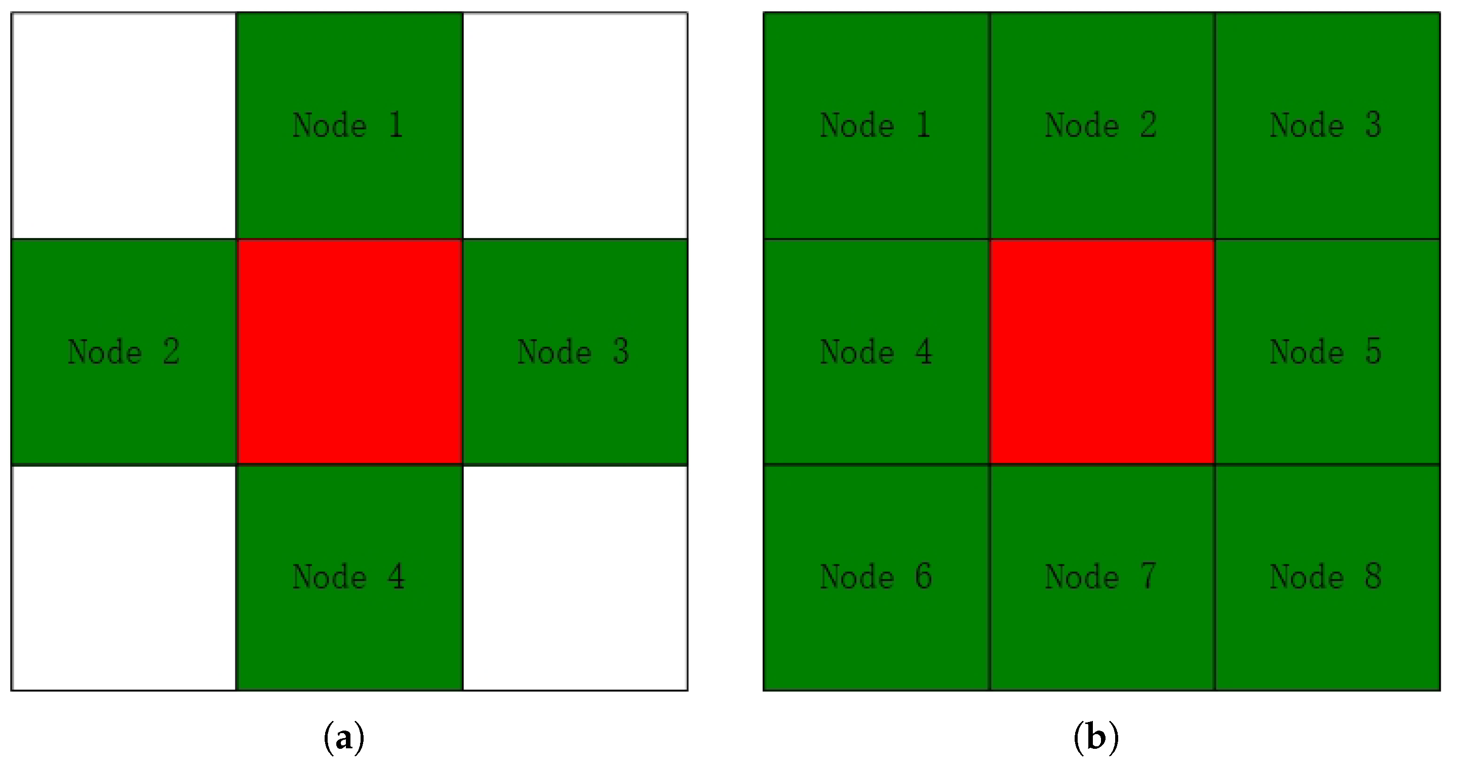
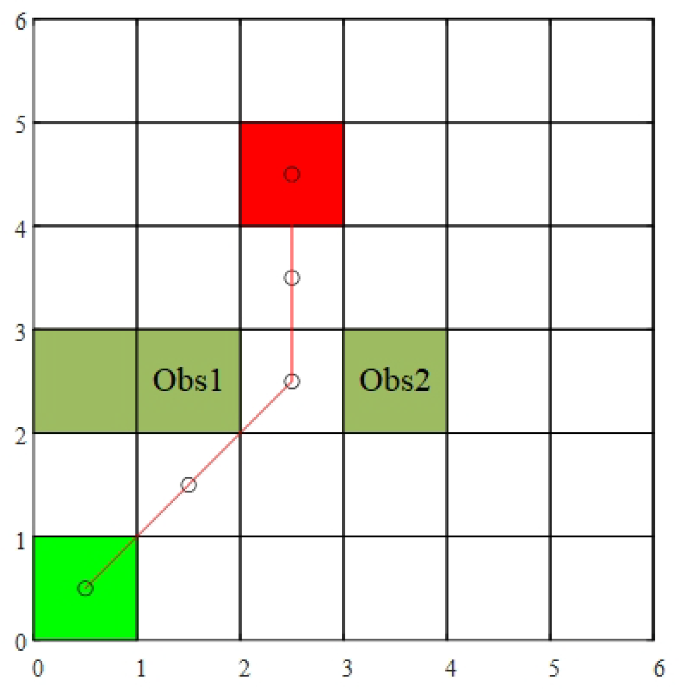
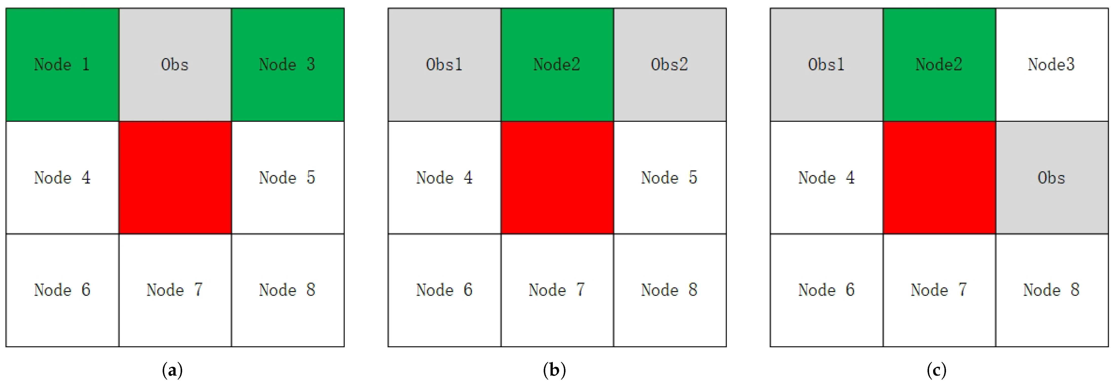
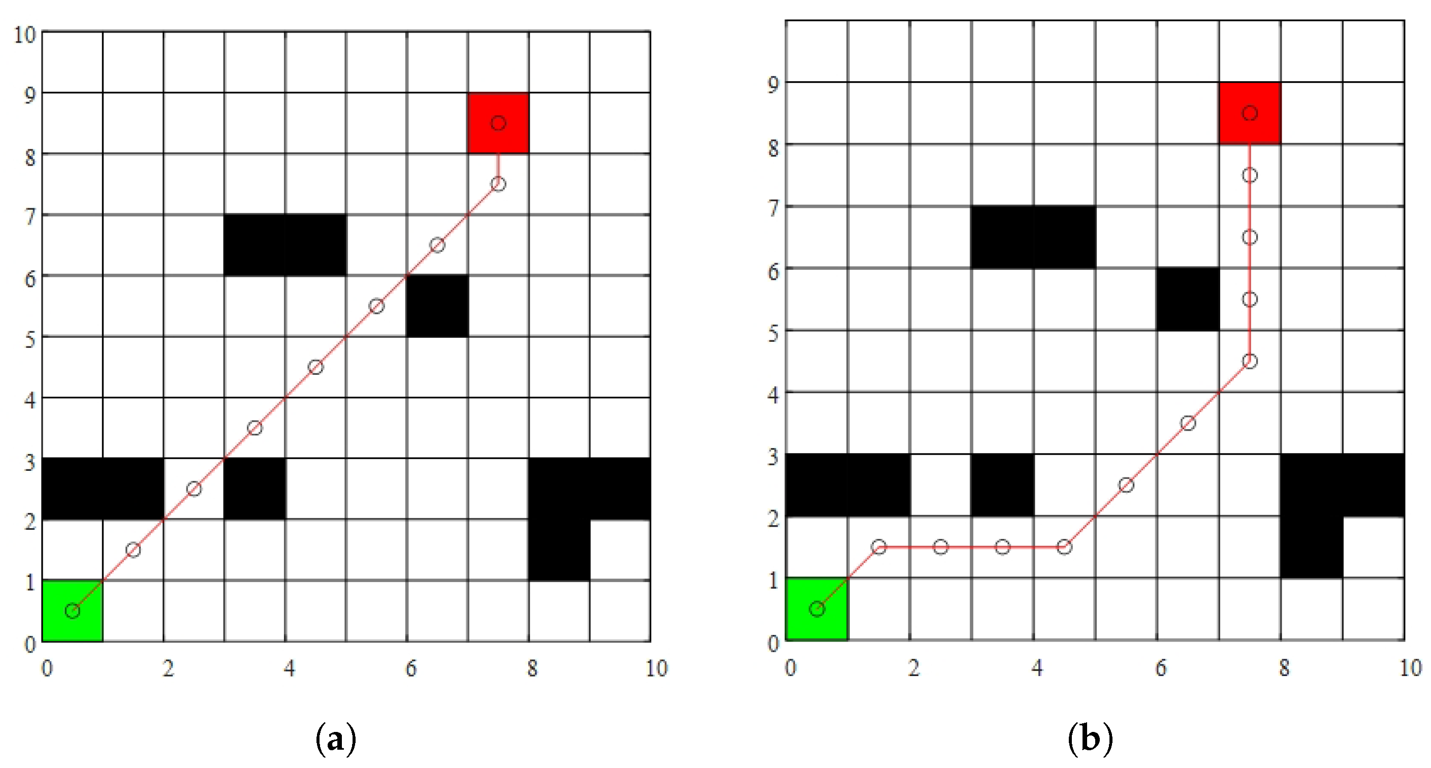
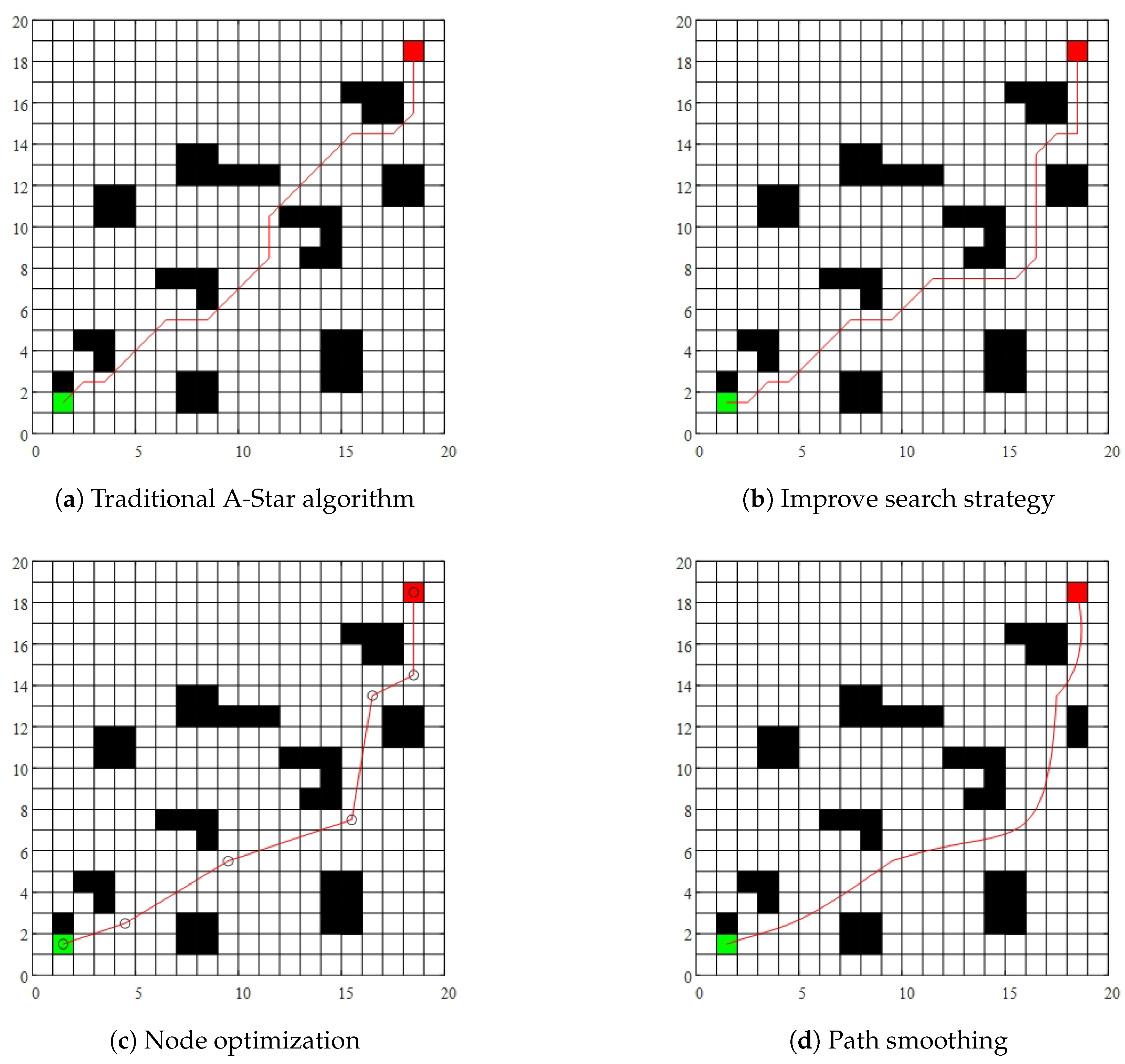
2.2. Improvement of Search Strategy

During the path planning process of the A-Star algorithm, the generated path may sometimes pass through the vertices of obstacles or narrow passages between obstacles, as shown in Figure 3.

As depicted in Figure 3, the planned path passes through the lower right corner of obstacle 1 and crosses the narrow passage between obstacle 1 and obstacle 2. Due to the underactuated nature of USVs, they are influenced by their limited control capabilities and external factors such as ocean currents during maneuvers, leading to deviations from the intended path. If the USV path is too close to an obstacle, the vessel must navigate near its edge, which poses significant safety risks. Similarly, when passing through narrow passages, the strong inertia of USVs makes them prone to collisions during turns, further threatening safe navigation.

To avoid the aforementioned situations, this paper proposes a strategy for optimizing the search neighborhood, with the specific optimization method as follows:  Firstly, traverse the eight adjacent nodes around the current parent node to determine its child nodes in the four basic directions (up, down, left, and right). If any of these four directions has a child node that is an obstacle, then the two adjacent nodes in that direction that are adjacent to the obstacle are defined as “dangerous nodes”, as shown in Figure 4a, where node 1 and node 3 are considered dangerous nodes. Similarly, if node 5 is an obstacle, nodes 3 and 8 will be considered dangerous nodes. In the path planning process, unmanned boats will avoid selecting the positions defined as dangerous nodes as the next parent nodes. Therefore, the path planning of unmanned boats can ensure that they will not cross the edge points of obstacles.

If any node in one of the four neighboring directions is not an obstacle node, it is necessary to further determine whether the two adjacent nodes in that direction are both obstacle nodes. As shown in Figure 4b, if node 2 is not an obstacle node, it is necessary to check whether nodes 1 and 3 are both obstacle nodes. If nodes 1 and 3 are both obstacle nodes, node 2 will be excluded when selecting the next parent node. Similarly, if node 5 is not an obstacle node, it is necessary to check whether nodes 3 and 8 are both obstacle nodes. If both nodes 3 and 8 are obstacle nodes, the possibility of node 5 being the next parent node is ruled out. If both node 1 and node 5 are obstacles, as shown in Figure 4c, the USV will not select node 2 as the new parent node during path planning. Similarly, if both node 2 and node 8 are obstacle nodes, the USV will not choose node 5 as its next driving path. The relationship between the position of obstacles and the elimination of nodes is shown in

Table 2. Node Position and Excluded Node Relationship Table.

Location of Obstacles	Excluded Path Points
Node 1, Node 5	Node 2
Node 2, Node 8	Node 5
Node 3, Node 7	Node 5
Node 5, Node 6	Node 7
Node 8, Node 4	Node 7
Node 7, Node 1	Node 4
Node 6, Node 2	Node 4
Node 4, Node 3	Node 2

.

In a 10 × 10 obstacle map, starting from (1,1) and ending at (8,9), simulation verification was conducted on the improved algorithm. The results are shown in Figure 5. In Figure 5, (a) represents the path planning result using the traditional A-Star algorithm, while (b) shows the result using the improved A-Star algorithm. The green square indicates the starting point, the red square indicates the endpoint, the black squares represent obstacle nodes, the red line represents the generated path, and the red circles along the path represent node positions.

From Figure 5, it is evident that the traditional A-Star algorithm encounters issues such as crossing obstacle edges and navigating narrow passages between obstacles. In contrast, the improved A-Star algorithm successfully avoids these issues, significantly enhancing the safety of USV navigation.

Due to the USV’s search strategy prioritizing the avoidance of hazardous areas, the generated path is longer compared with the original version. Additionally, the number of nodes has increased, leading to more frequent turns as some originally straight paths are now diverted for safety. To further enhance navigation efficiency and reduce potential risks, additional optimization of path nodes is needed to minimize turns during the USV’s journey, ultimately improving safety and stability.

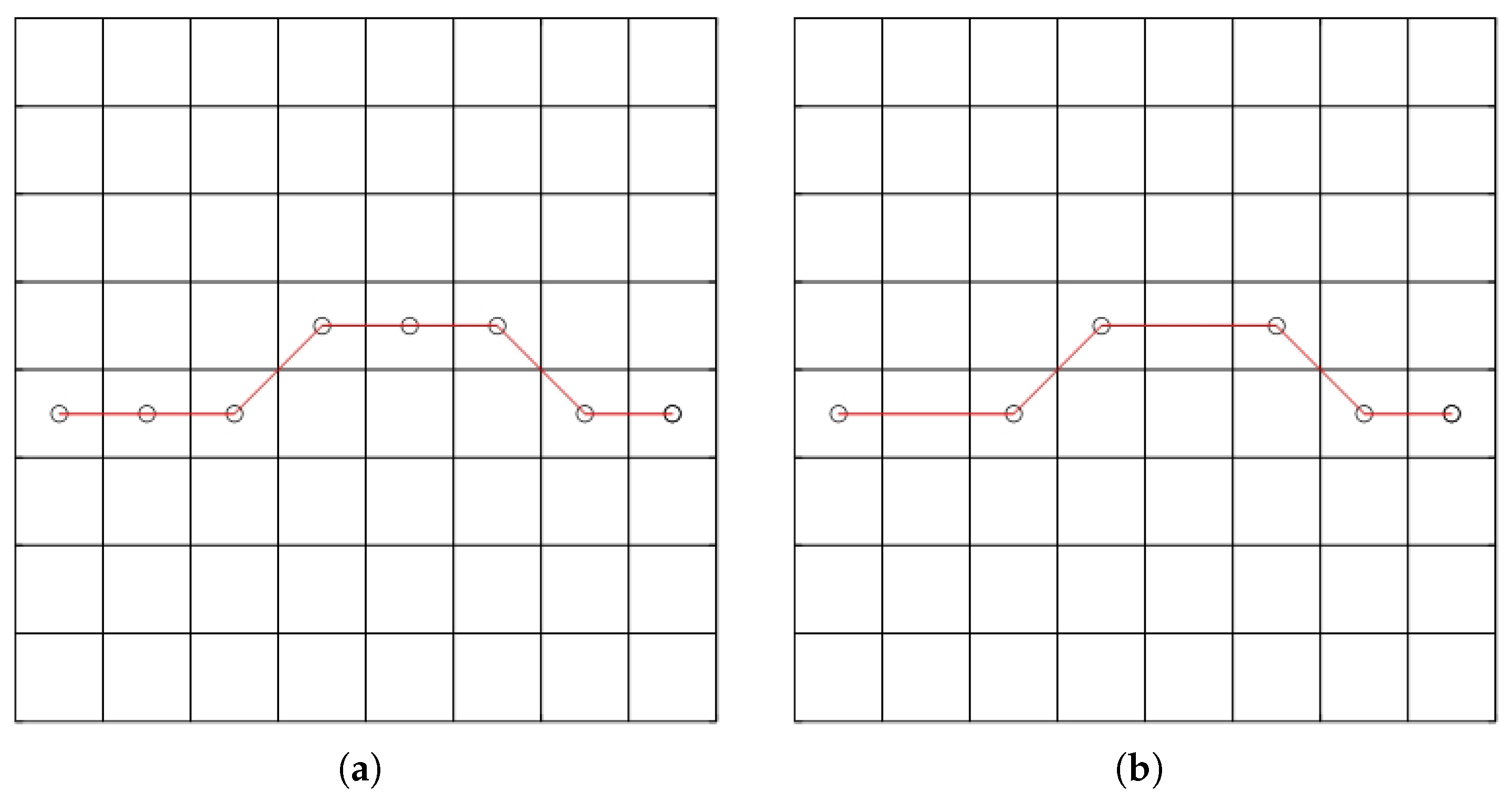
2.3. Node Optimization Strategy

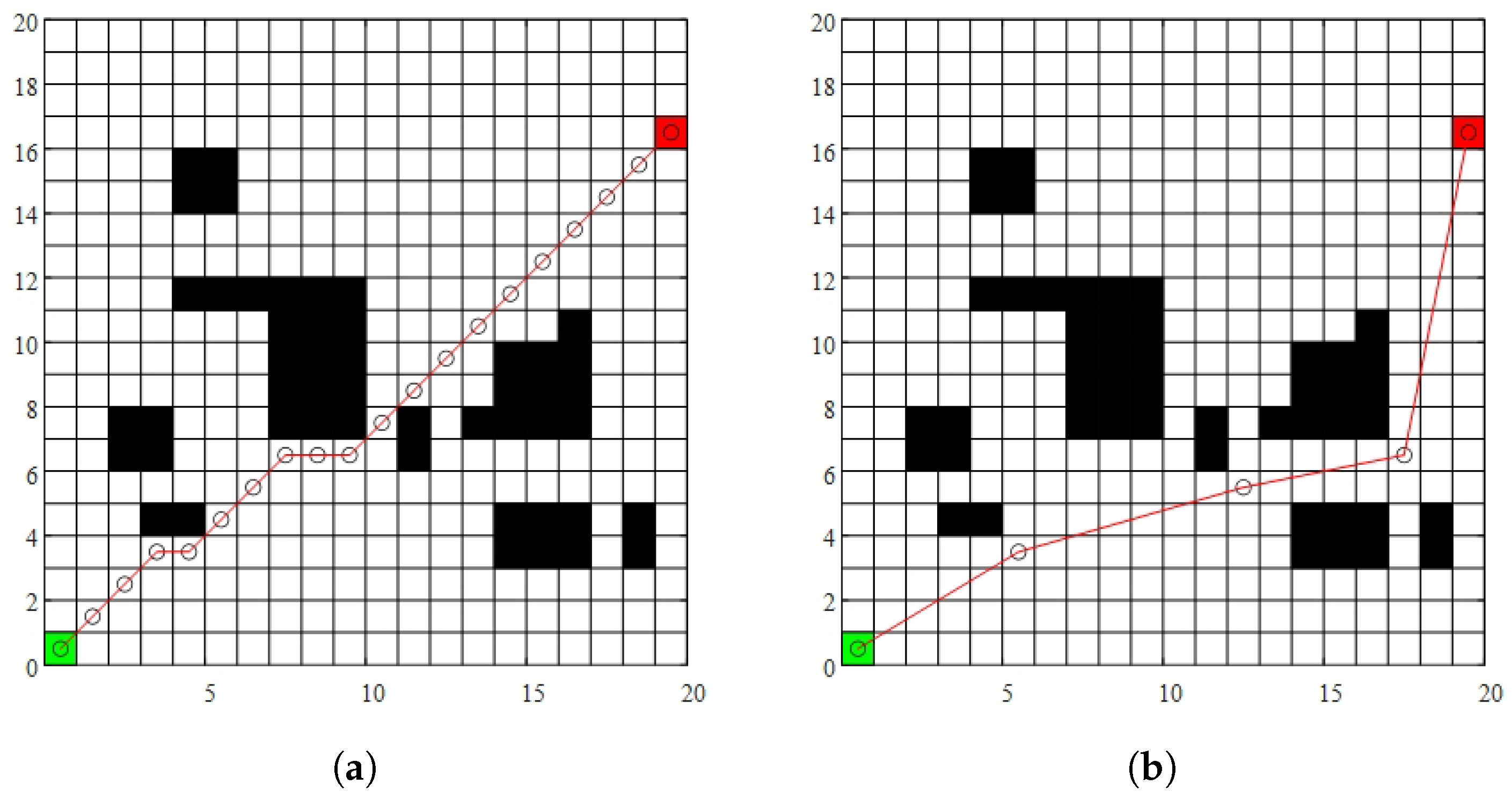
In Section 2.2, this paper optimized the search strategy of the A-Star algorithm. By comparing the path planning results before and after optimization, we observe that the optimized path improves safety and reduces the risk of USV navigation. However, this improvement also leads to an increase in path length and the number of turning points. Since USVs have strong inertia during turning and are influenced by external factors such as wind, waves, and ocean currents, excessive turning points can not only threaten the safety of unmanned vessels but also affect their long-term endurance.

To address this, further improvements were made specifically to reduce inflection points, aiming to shorten the path length. The optimization process follows these steps:

First, in the sequence of path points generated by optimizing the search strategy, we obtain nodes such as $n_0$, $n_1$, $n_2$, …, $n_i$, …, $n_g$, where $n_0$ is the starting point, $n_g$ is the ending point, and $n_i$ (with i ranging from 1 to $g-1$) represents each intermediate node. To optimize the path further, we perform preliminary processing on the nodes. Starting from $n_1$ and ending at $n_{g-1}$, we examine three consecutive nodes, $n_{i-1}$, $n_i$, and $n_{i+1}$, one by one. We check whether these points are collinear. If they are, node $n_i$ is redundant and can be removed. If the points are not collinear, $n_i$ is a necessary node and must be preserved. Figure 6 shows the schematic diagram of this process, where Figure 6a illustrates the path node situation before processing, and Figure 6b shows the situation after processing.

After the initial processing, the path remains unchanged, and the number of turns or turning angles does not decrease. Therefore, additional node processing is required to reduce the path length by decreasing the number of nodes. The specific method involves extracting the remaining nodes after the initial processing: $n_0$, $n_1$, $n_2$, …, $n_j$, $n_m$, where $n_0$ is the starting point, $n_m$ is the endpoint, and $n_j$ represents the intermediate nodes. Next, we randomly select three consecutive turning points, $n_{j-1}$, $n_j$, and $n_{j+1}$. The nodes $n_{j-1}$ and $n_{j+1}$ are then connected. If the connection passes through an obstacle (as shown in Figure 7a, node $n_j$ is retained; if the connection does not pass through an obstacle, node $n_j$ is marked as “Pending”.

Next, define the line connecting $n_{j-1}$ and $n_{j+1}$ as $l_1$, and draw two line segments $l_2$ and $l_3$, parallel to $l_1$, 0.4 units away from $l_1$ on both sides (as shown in Figure 7b. If any area between $l_2$ and $l_3$ intersects with the obstacle array, the path formed after deleting node $n_j$ is considered too close to the obstacle and does not meet the safety requirements for USV navigation. Therefore, node $n_j$ will not be deleted. If neither of the two line segments intersects with an obstacle, the path formed after deleting node $n_j$ is considered to maintain a safe distance from the obstacle, and node $n_j$ can be safely deleted.

We select a 20 × 20 grid map, with the starting point at (1,1) and the ending point at (20,17). On this map, simulation experiments were conducted on the node optimization method, and the results are shown in Figure 8. In Figure 8, (a) represents the path planning result using the traditional A-Star algorithm, while (b) represents the result using the node optimization method. Green represents the starting point, red represents the ending point, and black represents obstacle nodes.

By comparison, it is evident that after applying the improved search strategy and node optimization, the number of turning points in the path is significantly reduced. However, the path length has increased due to the USV maneuvering around hazardous obstacle areas to enhance navigation safety. Additionally, the USV maintains a safe distance from obstacles within the predefined safety threshold, ensuring secure obstacle avoidance and safe navigation. Despite these improvements, the optimized path still exhibits excessively sharp turns in some areas, which may affect maneuverability. Therefore, further path smoothing is required to generate a more continuous and navigable trajectory, ultimately enhancing the safety and stability of the USV’s navigation.

2.4. Path Smoothing

The mathematical basis of the Bézier curve is derived from the Bernstein polynomial, named after Russian mathematician Sergei Natanovich Bernstein (Farin, 2014) [35].

The Bézier curve is widely used in path planning due to its smoothness and ease of computation, transforming the problem of curve shaping into the solution of coordinate points. However, paths planned on grid maps often contain many bends and sharp corners, which may cause USVs to make frequent sharp turns or even stop moving during their journey. This instability not only reduces the operational efficiency of the USV but also increases energy consumption and threatens navigation safety [36]. As a result, an increasing number of researchers are turning to Bézier curves for path smoothing. Compared with other smoothing algorithms, Bézier curves offer significant advantages in generating curves with continuous curvature [37].

The definition of a first-order Bézier curve: Given two points $P_0$ and $P_1$, a first-order (or linear) Bézier curve is a straight line connecting these two points, which can be given by the following equation and is equivalent to the result of linear interpolation:

$$B\left(t\right)=(1-t)P_0+t{P}_1,t\in [0,1],$$

(5)

where t is the interpolation parameter. When $t=0$, the curve is at point $P_0$, and when $t=1$, the curve is at point $P_1$. For any $t\in (0,1)$, the curve lies on the straight line connecting $P_0$ and $P_1$.

Similarly, if given a total of $n+1$ control points $C_0,C_1,\dots ,C_m,\dots ,C_n$, the formula for an M-order Bézier curve can be expressed by the following equation:

$$B\left(t\right)=\sum _{m=0}^n{\displaystyle \frac{n!}{m!(n-m)!}}{C}_m{(1-t)}^{n-m}{t}^m,t\in [0,1]$$

(6)

where, $C_m$ represents the coefficient or weight of control points, and the range of t is $[0,1]$. It represents the number of points that control the generation of Bézier curves. The smaller the value, the smaller the step size, and the more points generated.

If the listing is regarded as a parametric equation belonging to the following equation, the curvature of each point in the point set generated by the Bézier curve can be represented by the following equation. Here, $B_x^{\prime }\left(t\right)$ is the first derivative of parameter t in the x direction, $B_y^{\prime }\left(t\right)$ is the first derivative of parameter t in the y direction, and $B^{″}\left(t\right)$ is the second derivative of parameter t in the x or y direction.

$$\begin{array}{cc}\hfill x& =B_x^{\prime }\left(t\right)\hfill \end{array}$$

(7)

$$\begin{array}{cc}\hfill y& =B_y^{\prime }\left(t\right)\hfill \end{array}$$

(8)

$$\begin{array}{cc}\hfill \rho & ={\displaystyle \frac{B_x^{\prime }\left(t\right)B_y^{″}\left(t\right)-B_y^{\prime }\left(t\right)B_x^{″}\left(t\right)}{{\left({\left(B_x^{\prime }\left(t\right)\right)}^2+{\left(B_y^{\prime }\left(t\right)\right)}^2\right)}^{3/2}}}\hfill \end{array}$$

(9)

If the curvature is a positive number, then the direction of the curve is concave; otherwise, it is convex.

This article proposes a path smoothing method based on Bezier curves. This method takes the discrete path nodes generated by the A-Star algorithm in Section 2.3 as input and uses segment-by-segment smoothing to optimize the smoothness and safety of the path.

The specific implementation plan of the method proposed in this article is as follows:

• Node extraction: Extract a series of optimized path nodes $n_1$,$n_2$,$n_3$,…,$n_m$ from Section 2.3. Starting from the starting point $n_1$, divide these nodes into three consecutive groups of three nodes each. For example, the first group $\{n_1,n_2,n_3\}$, $\{n_3,n_4,n_5\}$. If there are $2k$(where k is a positive integer) nodes and there is only one node left that cannot form three nodes, then $\{n_{m-1},n_m,\}$ is taken as a group. If there are $2k+1$ nodes in total, they can be divided into groups of three. Each group of three nodes will be used to generate a Bézier curve.
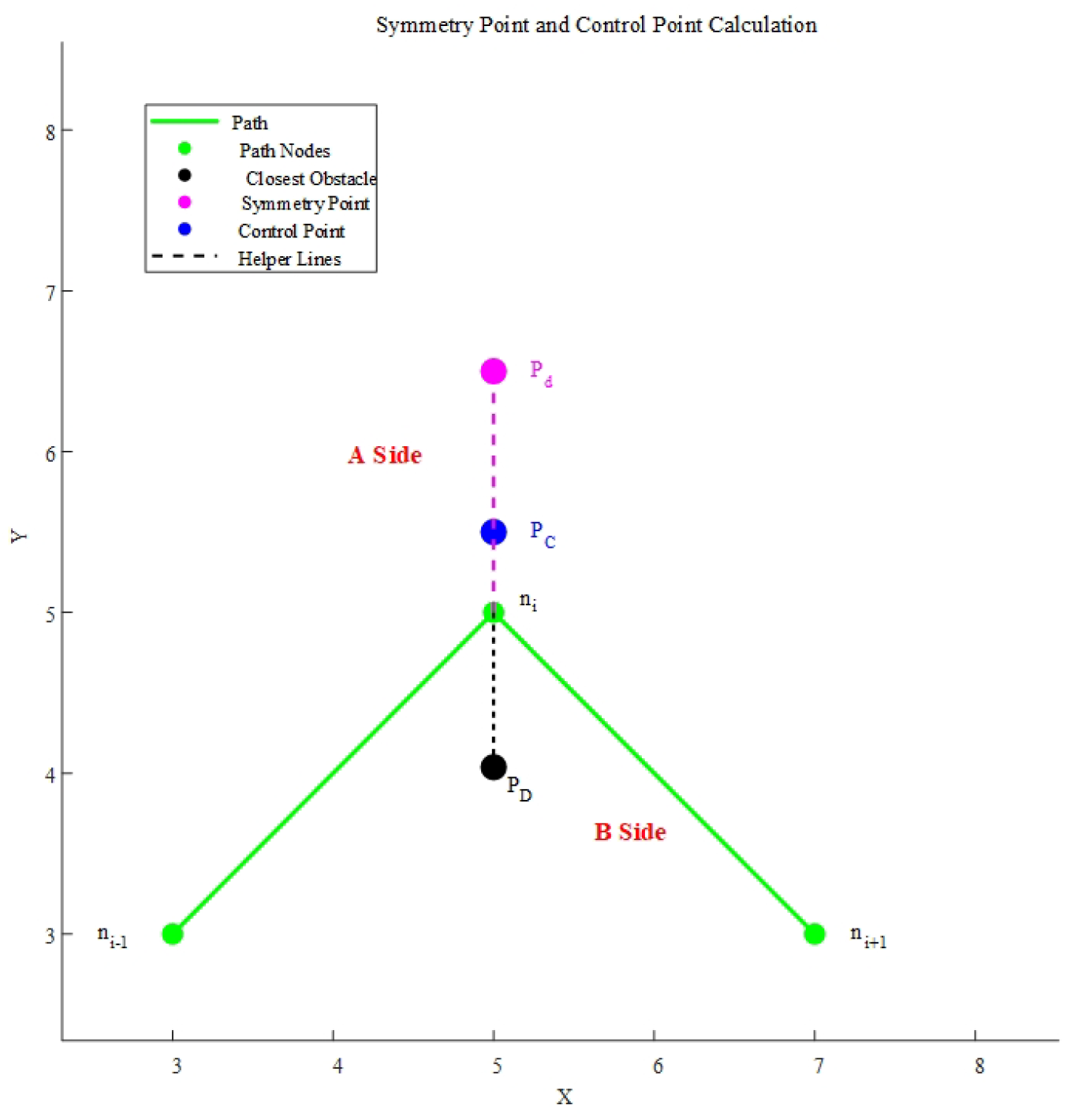
• Selection of control points: The position of control points is crucial for path smoothness and obstacle avoidance performance. This paper proposes a dynamic adjustment method based on obstacle distribution. Select a set of nodes from the previous step, $\{n_{i-1},n_i,n_{i+1}\}$. Define the path composed of this group of nodes as $s_1$. Select the middle node $n_i$, check the obstacles on both sides of path $s_1$, and calculate the distance between the obstacles on both sides and the middle node $n_i$. Calculate the distance $d_L$ from the obstacle on side A to $n_i$, and calculate the distance $d_R$ from the obstacle on side B of the path to $n_i$. Determine the difference between $d_R$ and $d_L$. If $d_R<d_L$, it indicates that the intermediate node $n_i$ is closer to the obstacle on side B, and the control point needs to be shifted to side A to ensure the path avoids the obstacle. Conversely, if $d_R\ge d_L$, the control point should be shifted to side B.
  Assume that the nearest obstacle coordinate to $n_i$ is $P_D$. The control point $P_C$ can be determined by calculating the symmetry point $P_d$ of $n_i$ and $P_D$. The formula for $P_d$ is

  $$P_d=2n_i-P_D$$

  (10)
  If $n_i=(x_i,y_i)$ and $P_D=(x_D,y_D)$, then

  $$P_d=(2x_i-x_D,2y_i-y_D)$$

  (11)
  The final position of the control point $P_C$ is chosen between the middle node $n_i$ and the symmetry point $P_d$. Specifically,

  $$P_C={\displaystyle \frac{2}{3}}{n}_i+{\displaystyle \frac{1}{3}}{P}_d$$

  (12)
  This formula ensures that the control point is biased towards one-third of the distance between the middle node and the symmetry point, thereby controlling the smoothness of the path while effectively avoiding obstacles. Figure 9 illustrates the method for selecting control points for the Bézier curve, where $P_D$ represents the obstacle closest to node $n_i$, $P_d$ denotes the symmetry point of $P_D$ relative to $n_i$, and $P_C$ represents the position of the control point.
  If there are only $2k$ nodes in the path, the last two points cannot form a set of three nodes, so no control points are added, and the last two points $\{n_{m-1},n_m\}$ are directly smoothed to form the path. When the distance between the obstacle and the intermediate node $n_i$ is greater than 1.5 grid sizes, the surrounding environment of the node is considered relatively safe, and no additional control points are needed. In this case, the nodes are directly used for path smoothing without introducing additional control points, ensuring the smoothness of the path while avoiding unnecessary complex calculations.

3. Dynamic Obstacle Avoidance

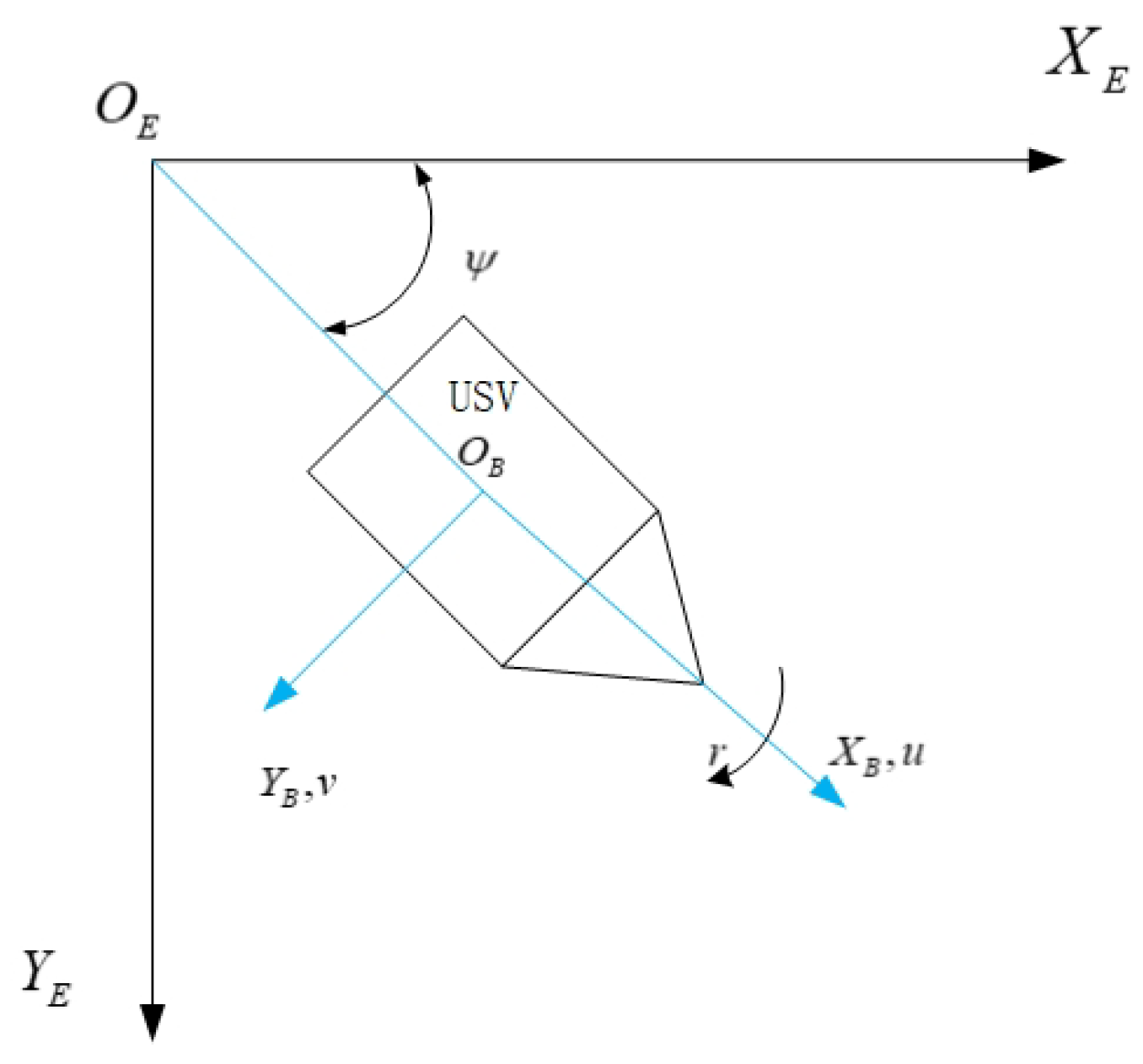
3.1. Modeling of Unmanned Surface Vessels

In order to accurately describe the motion of unmanned boats, it is necessary to establish a reference coordinate system for unmanned boats. Because this article mainly focuses on the path planning of USVs and conducts simulation experiments in a grid map, only a three-degree-of-freedom model needs to be established in this article. Therefore, this article does not consider the roll, pitch, and heave motion models of the USV. The modeling of the three-degree-of-freedom USV model is shown in Figure 10, where $O_E{X}_E{Y}_E$ represents its inertial coordinate axis. The $O_E{X}_E$ axis and $O_E{Y}_E$ axis are both parallel to the horizontal plane, pointing towards the geographical east and north directions, respectively. The attached coordinate system is $O_B{X}_B{Y}_B$, and the origin $O_B$ is usually defined as the center of mass of the unmanned vessel. The $O_B{X}_B$ axis and $O_B{Y}_B$ axis are both parallel to the sea level, pointing from the origin to the bow and starboard of the unmanned vessel, respectively. Among them, u represents its longitudinal linear velocity, v represents its lateral linear velocity, and r represents its yaw angular velocity. $\psi$ represents the deflection angle of the USV relative to the inertial coordinate system. As this article focuses on USV path planning and adopts simulation verification, its kinematic characteristics are the key factor in the path planning process, mainly focusing on the motion state and geometric relationship of USVs. Therefore, in order to simplify the model and improve computational efficiency, this study is based solely on the kinematic three-degree-of-freedom model, without considering complex dynamic characteristics such as hydrodynamic effects, inertia moments, etc. In most planar path planning and obstacle avoidance scenarios, kinematic models can accurately describe the motion characteristics of USVs in a two-dimensional plane, especially under low-speed or medium-speed operating conditions. Due to the fact that motion planning algorithms (such as the dynamic window method) mainly rely on kinematic constraints for local optimization, the impact of dynamic modeling on this study is relatively small, so dynamic modeling is omitted. Therefore, the three-degree-of-freedom kinematic model of its USV is

$$\dot{\eta }=J\left(\eta \right)\upsilon$$

(13)

where $\eta ={\left[\begin{array}{c}xy\psi \end{array}\right]}^T$ is the Euler angle vector, and v represents the angular velocity vector, and $J\left(\eta \right)$ is the transformation matrix. Its specific definition is

$$J\left(\eta \right)=\left[\begin{array}{ccc}cos\psi & -sin\psi & 0\\ sin\psi & cos\psi & 0\\ 0& 0& 1\end{array}\right]$$

(14)

Therefore, the motion equation of the kinematic model with three degrees of freedom is

$$\left\{\begin{array}{c}\dot{x}=ucos\psi -vsin\psi ,\hfill \\ \dot{y}=usin\psi -vcos\psi ,\hfill \\ \dot{\psi }=r\hfill \end{array}\right.$$

(15)

Therefore, the state of its system can be represented as $(u,v,x,y,\psi ,r)$.

3.2. Dynamic Window Approach

The Dynamic Window Approach (DWA) is a method based on predictive control theory that can safely and effectively avoid obstacles in unknown environments. It also has the advantages of low computational complexity and rapid response. The principle is to first collect velocity samples of the robot through the mathematical model of the USV, predict and simulate the motion trajectory of the robot in the next time period under the sample velocity, and evaluate these motion trajectories to ultimately select the optimal path. The USV moves according to the optimal path, and its motion posture and direction are determined by the current linear velocity and angular velocity of the USV. The DWA algorithm mainly includes three steps: velocity sampling, trajectory prediction, and trajectory evaluation.

3.2.1. Speed Sampling

Due to the inherent characteristics of the USV and environmental constraints, the USV’s speed has certain boundary limitations. The achievable speed space $V_m$ can be expressed as

$$V_m=\{(v,\omega )\mid v\in (v_{\min },v_{\max }),\omega \in ({\omega }_{\min },{\omega }_{\max })\}$$

(16)

where $v_{\min }$ and $v_{\max }$ represent the minimum and maximum linear velocities of the USV, and ${\omega }_{\min }$ and ${\omega }_{\max }$ represent the minimum and maximum angular velocities.

Since the USV is motor-driven, both its linear acceleration and angular acceleration are subject to certain limitations. Therefore, the speed space considering acceleration, denoted as $V_d$, is given by:

$$V_d=\left\{(v,\omega )\mid \begin{array}{c}v\in [v_t-v_{\mathrm{a}\max }·\mathrm{\Delta }t,v_t+v_{\mathrm{a}\max }·\mathrm{\Delta }t]\hfill \\ \omega \in [{\omega }_t-{\omega }_{\mathrm{a}\max }·\mathrm{\Delta }t,{\omega }_t+{\omega }_{\mathrm{a}\max }·\mathrm{\Delta }t]\hfill \end{array}\right\}$$

(17)

where $v_t$ and ${\omega }_t$ represent the linear and angular velocities at the current time, and $v_{\mathrm{a}\max }$ and ${\omega }_{\mathrm{a}\max }$ represent the maximum linear and angular accelerations of the USV. In this paper, the DWA algorithm is used for dynamic obstacle avoidance. Therefore, it is necessary to consider the obstacles around the USV during the dynamic avoidance process. The constraint conditions for ensuring that the USV does not collide with obstacles during a specific dynamic avoidance process can be expressed as

$$V_a=\left\{(v,\omega )\mid \begin{array}{c}v\in [v_{\min },\sqrt{2·\mathrm{dist}(v,\omega )·v_{\mathrm{a}\max }}]\hfill \\ \omega \in [{\omega }_{\min },\sqrt{2·\mathrm{dist}(v,\omega )·{\omega }_{\mathrm{a}\max }}]\hfill \end{array}\right\}$$

(18)

where $\mathrm{dist}(v,\omega )$ represents the minimum distance between the simulated trajectory corresponding to the current velocity and the surrounding obstacles. It is defined as

$$\mathrm{dist}(v,\omega )=min({\mathrm{dist}}_d(v,\omega ),{\mathrm{dist}}_s(v,\omega ))$$

(19)

where ${\mathrm{dist}}_d(v,\omega )$ represents the distance between the USV and dynamic obstacles, and ${\mathrm{dist}}_s(v,\omega )$ represents the distance to surrounding static obstacles. When the dynamic obstacle trigger condition is not met, $\mathrm{dist}(v,\omega )$ only considers the velocity constraints from static obstacles. Once the dynamic avoidance condition is triggered, $\mathrm{dist}(v,\omega )$ is controlled by both ${\mathrm{dist}}_d(v,\omega )$ and ${\mathrm{dist}}_s(v,\omega )$.

Thus, the final USV velocity sampling space is the intersection of the three velocity spaces:

$$V_S=V_m\cap V_d\cap V_a$$

(20)

3.2.2. Trajectory Prediction

At each time step $\mathrm{\Delta }t$, the kinematic equations are used to update and determine the USV’s position and heading angle at the next time step. Based on the current state space equations, the USV’s state at the next time step can be calculated using the following equations:

$$\left\{\begin{array}{c}{x}_{t+1}=x_t+\dot{x}\mathrm{\Delta }t=x_t+(vcos\psi -vsin\psi )\mathrm{\Delta }t\hfill \\ y_{t+1}=y_t+\dot{y}\mathrm{\Delta }t=y_t+(vsin\psi -vcos\psi )\mathrm{\Delta }t\hfill \\ {\psi }_{t+1}={\psi }_t+\dot{\psi }\mathrm{\Delta }t={\psi }_t+r\mathrm{\Delta }t\hfill \end{array}\right.$$

(21)

The core of the prediction estimation is trajectory sampling. Suppose we select a time period T and perform continuous sampling over time intervals, which allows us to predict a series of future trajectory points. In all simulations conducted in this paper, we take $T=0.1$. During the prediction process, in addition to calculating the trajectory, we must also check whether the predicted trajectory at the next time step collides with any obstacles. If a predicted trajectory point collides with an obstacle, we consider the current velocity combination unacceptable and need to re-select a new velocity combination to avoid the obstacle.

3.2.3. Evaluation Function

After determining the robot’s constrained speed range, some of the simulated trajectories are feasible. However, too many trajectories can make the navigation decisions of the USV confusing. Therefore, it is necessary to evaluate and select the best trajectories from the sampled ones. The evaluation function is used to select the optimal trajectory corresponding to the speed as the driving speed. The evaluation function can be expressed as a weighted sum of multiple subfunctions, each of which addresses a specific performance criterion, including heading deviation, obstacle distance, the current linear and angular velocities of the USV, and the predicted time of the trajectory. Each speed combination generates a predicted trajectory, and during the trajectory prediction process, we need to calculate the distance between each trajectory point and the obstacles. If at any time the trajectory collides with an obstacle, it indicates that the current velocity combination is infeasible. Therefore, the evaluation function needs to assess all trajectories and discard the infeasible ones.

Finally, for each feasible trajectory, the following weighted evaluation function is used for scoring:

$$f(v,\omega )=\alpha ·h(v,\omega )+\beta ·d(v,\omega )+\gamma ·s(v,\omega )+\delta ·t(v,\omega )$$

(22)

where $\alpha ,\beta ,\gamma ,\delta$ are the weight coefficients of the evaluation function, controlling the relative importance of each evaluation item. By calculating the evaluation value of each trajectory generated by the velocity combination, the trajectory with the highest evaluation value is selected as the optimal trajectory. The velocity combination corresponding to the optimal trajectory will be used as the driving command for the USV to move towards the target.

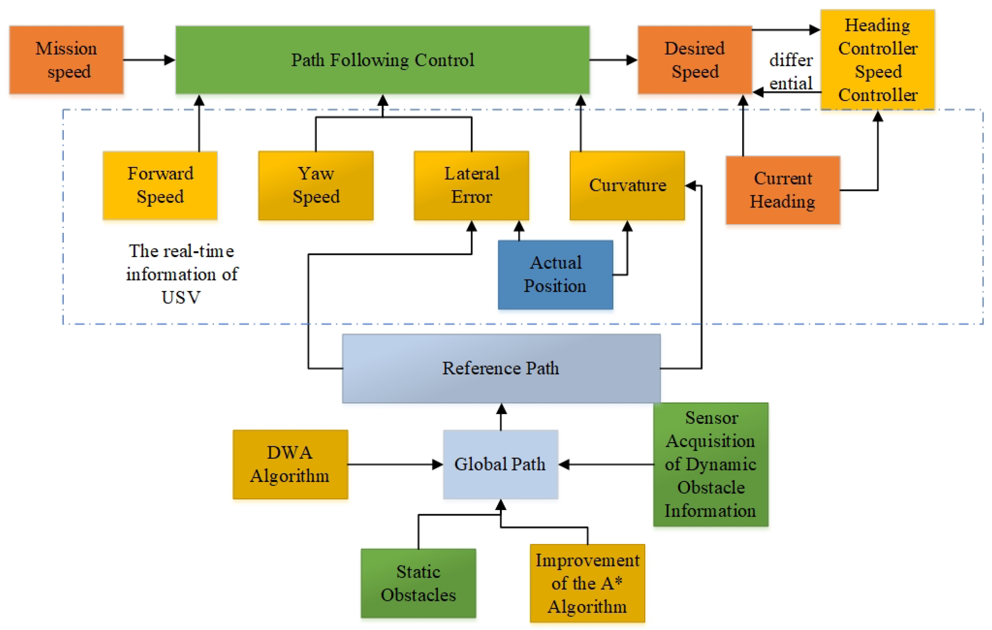
3.3. Control System Design and Architecture

The control system block diagram is shown in Figure 11.

4. Simulation

In this study, we used MATLAB 2024a for simulation and analysis, with the experimental environment running on an Intel^® Core™ i5-10300H CPU @ 2.50 GHz processor and equipped with 8.0 GB of memory. The environment modeling adopts a grid map, where the grid size is set to 1, and the heuristic function uses Manhattan distance. The robot radius is set to 0.1, and the safe radius is 0.4. In the visual representation of the grid map, green squares represent the starting point, red squares represent the ending point, and black squares represent static obstacle nodes. The position and size of all static obstacles are fixed and known.

In all simulation experiments in this chapter, the computation time of the algorithm may fluctuate even under the same conditions due to factors such as CPU frequency and memory usage. Therefore, to ensure the stability and reliability of the data, we took the average of 50 program runs as the final running time of the algorithm. In addition, the unit of path length is consistent with the grid size and is used to measure the actual distance traveled by robots in the environment.

Although the simulations in this study were conducted in MATLAB on a high-performance Intel^® Core™ i5-10300H CPU with 8 GB of memory, real-world USVs rely on embedded systems with limited computational resources. These systems, typically ARM-based SoCs, have constraints such as reduced memory and real-time operating system requirements, which may impact the performance of path planning algorithms. The slower computation speed on such platforms may affect the USV’s ability to react to dynamic obstacles in real-time, compromising safety and efficiency.

To ensure the proposed algorithm runs efficiently on embedded platforms, future work should focus on optimizing the algorithm for the limited processing power and memory available. This could involve restructuring the algorithm, reducing heuristic calculation frequency, and using more compact grid representations to reduce memory usage. Additionally, hardware accelerators like GPUs or FPGAs may be leveraged to improve computational speed while respecting memory constraints. Testing on embedded platforms is essential to assess the algorithm’s real-world performance and its ability to meet real-time constraints in USV operations.

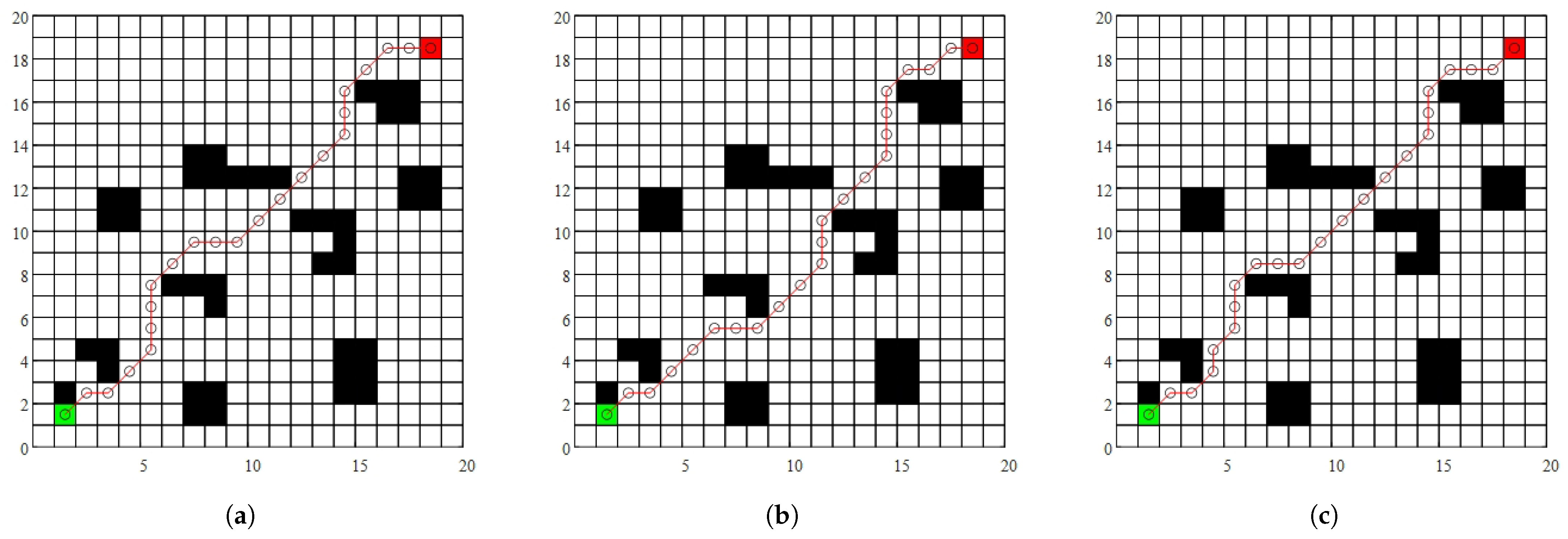
4.1. Simulation Results of Various Improvements in Global Path Planning

Simulation experiments were conducted using 20 × 20 grid maps with starting points of (2,2) and ending points of (19,19). The detailed result data are shown in

Table 3. Comparison of various improved path planning data in global path planning.

Algorithms	Turning Points	Path Length	Planning Time	Smoothness
A-Star	9	26.97	0.325	Unsmooth
Improvement 1	11	29.31	0.078	Unsmooth
Improvement 2	5	27.64	0.068	Unsmooth
Improvement 3	5	27.17	0.071	smooth

, and the path drawing results are shown in Figure 12. The simulation experiment includes the following scenarios: traditional A-Star algorithm, A-Star algorithm with improved search strategy, A-Star algorithm with improved search strategy and node optimization, and A-Star algorithm with improved search strategy, node optimization, and path smoothing. The last three improvements are replaced by improvement 1, improvement 2, and improvement 3, respectively.

Compared with the traditional A-Star algorithm in Figure 12a, the algorithm generated by the improved search strategy in Figure 12b no longer crosses the vertices of obstacles and avoids the situation of crossing narrow channels between obstacles, making the path safer. However, the cost of the path is that the length of the path increases, and the number of turning points also increases. This is because the improved algorithm requires the original straight path to take a detour, changing the path that originally diagonally passes through obstacles to two straight lines that need to turn. As a result, the generated path becomes longer and the number of turning points increases accordingly.

Figure 12c shows that through further node optimization, the number of turning points in the path is significantly reduced, and the path length is shortened. This is because node optimization merges multiple line segments into a straight line, reducing the number of nodes in the path and making it relatively shorter. However, the planned path still has some unevenness.

After the curve smoothing process in Figure 12d, the path length is further shortened and the path becomes smoother, which can effectively meet the kinematic characteristics of the USV and avoid unexpected situations such as collisions caused by USV inertia and rigidity. In addition, the generated path always maintains a safe distance from obstacles, greatly improving the safety of the path.

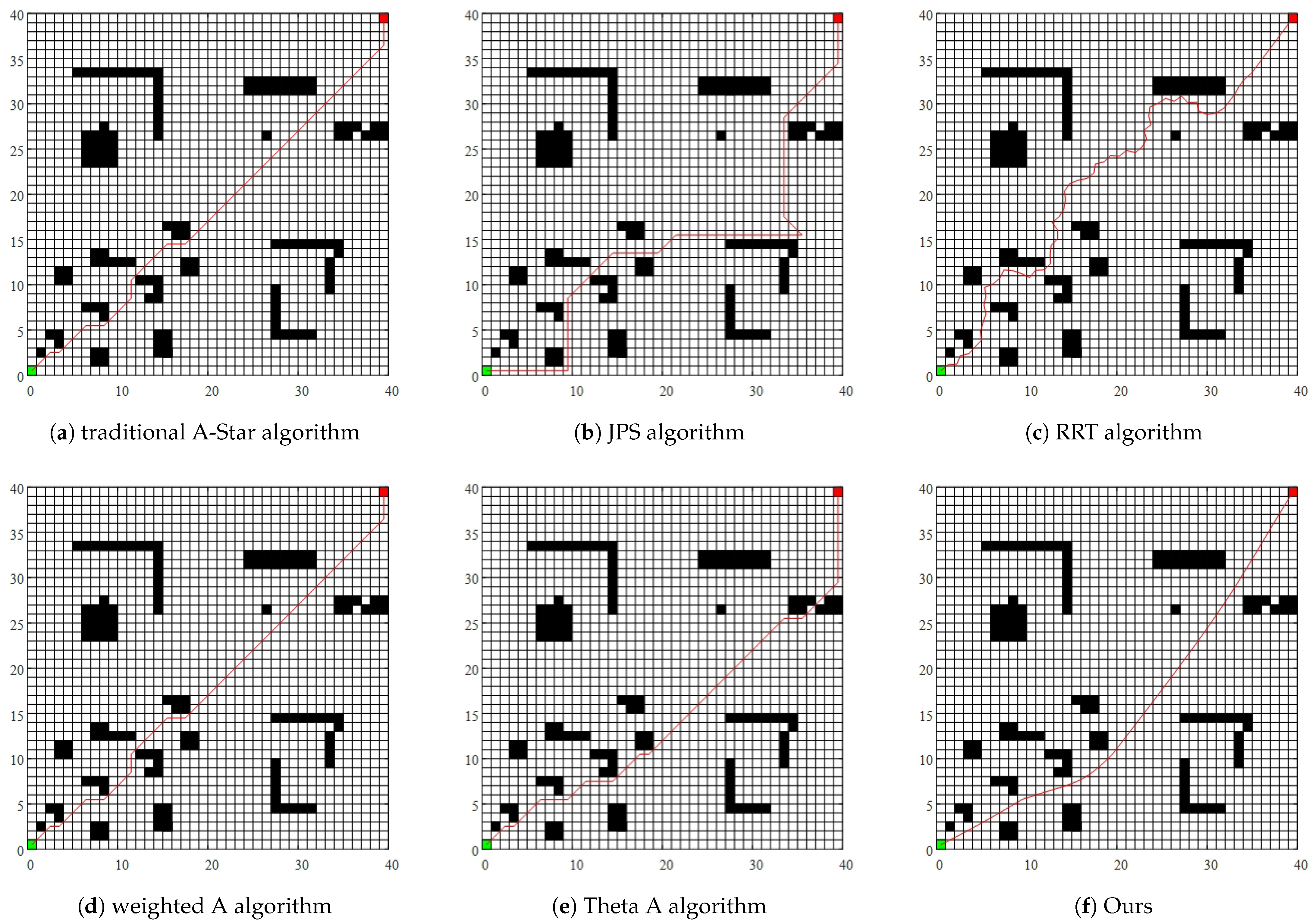
4.2. Comparison with Other Algorithms

Conduct simulation experiments on a 40 × 40 grid map, starting from (1,1) and ending at (40,40). Apply the traditional A-Star algorithm, JPS algorithm, RRT algorithm, Weighted A algorithm, Theta A algorithm, and the algorithm proposed in this paper for path planning. The path planning results are shown in Figure 13, and detailed data can be found in

Table 4. Comparison results of different algorithm path planning and data comparison.

Algorithms	Turning Points	Path Length	Planning Time	Smoothness
A-Star	9	58.08	0.312	Unsmooth
JPS	9	73.21	0.075	Unsmooth
RRT	58	68.00	0.044	Unsmooth
weight A	9	58.08	0.032	Unsmooth
Theta A	11	61.01	0.082	Unsmooth
ours	5	56.13	0.143	smooth

. The principles and advantages of these algorithms are discussed in detail in the Introduction. The selection of these algorithms for comparison is based on the following reasons: The A* algorithm serves as a baseline to validate the improvements made in search strategy, node optimization, and path smoothing. The JPS algorithm is used to demonstrate the improvements in computational efficiency and turning angles achieved by the proposed algorithm. The Weighted A* and Theta A* algorithms are employed to evaluate the enhancements in path smoothness and computational efficiency. The inclusion of the RRT algorithm allows for a comprehensive comparison, effectively highlighting the advantages of the proposed algorithm in path planning for complex static environments, while also emphasizing the comparison in terms of path smoothness.

Compared with the A-Star algorithm, the proposed algorithm significantly reduces the number of nodes and shortens the path length, improving both the efficiency and practicality of the path planning process. The A-Star algorithm, while effective in many cases, suffers from certain limitations, including the issue of crossing obstacle vertices and producing paths that are too close to obstacles. This can compromise the safety of USV, especially in complex and dynamic environments. On the other hand, the proposed algorithm avoids such issues by refining the path and optimizing the search strategy, although it comes with a slight increase in planning time.

When compared with the JPS algorithm, the proposed method demonstrates clear advantages in both the number of nodes and the overall path length. The JPS algorithm, while avoiding the problem of crossing obstacle vertices, generates paths with many inflection points and sharp turning angles. These sharp turns make the path less suitable for USVs, as they do not meet the actual navigation requirements, which demand smooth and stable movement, especially in environments where obstacles and dynamic factors are prevalent.

In comparison with the RRT algorithm, which is widely used in various path planning applications, the proposed algorithm outperforms it in terms of path length and number of inflection points. The RRT algorithm typically results in paths with the highest number of inflection points and longer path lengths, which makes it less suitable for safe path planning for USVs. The algorithm generates paths that are not optimized for efficiency, leading to increased travel time and potential navigation hazards. Furthermore, the path generated by the Weighted A* algorithm on this map is very similar to that of the A-Star algorithm, although it has a slightly longer planning time. Despite the similarity in path generation, the Weighted A* algorithm has some advantages in terms of handling obstacles more effectively.

The Theta* algorithm also presents some issues, particularly in the case of crossing oblique points and dealing with narrow gaps between obstacles. These factors make the Theta* algorithm less effective for USV path planning, as it negatively impacts the navigation safety and stability. Overall, the algorithm proposed in this paper demonstrates superior performance in terms of both path length and the number of nodes, even though the planning time is slightly longer compared with other algorithms. Its ability to generate smoother paths with fewer turns makes it more suitable for practical USV navigation, especially in real-world environments with dynamic obstacles.

Compared with other algorithms such as A-Star, the most significant feature of the proposed algorithm is its ability to effectively avoid complex obstacle areas, opt for detours when necessary, and generate smoother and safer paths. This not only improves the safety of USV navigation but also enhances operational efficiency by minimizing unnecessary turns and avoiding potential collisions with obstacles.

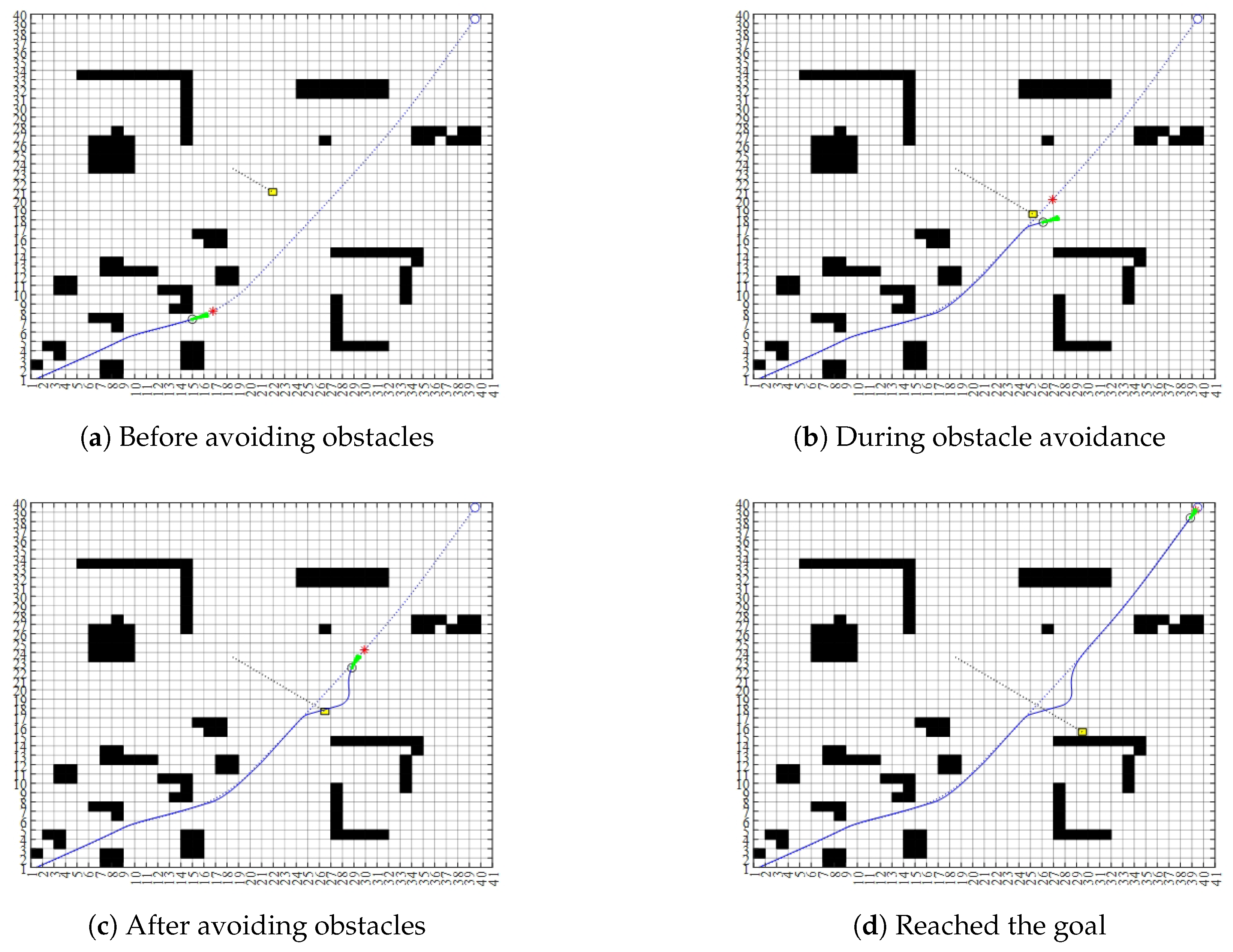
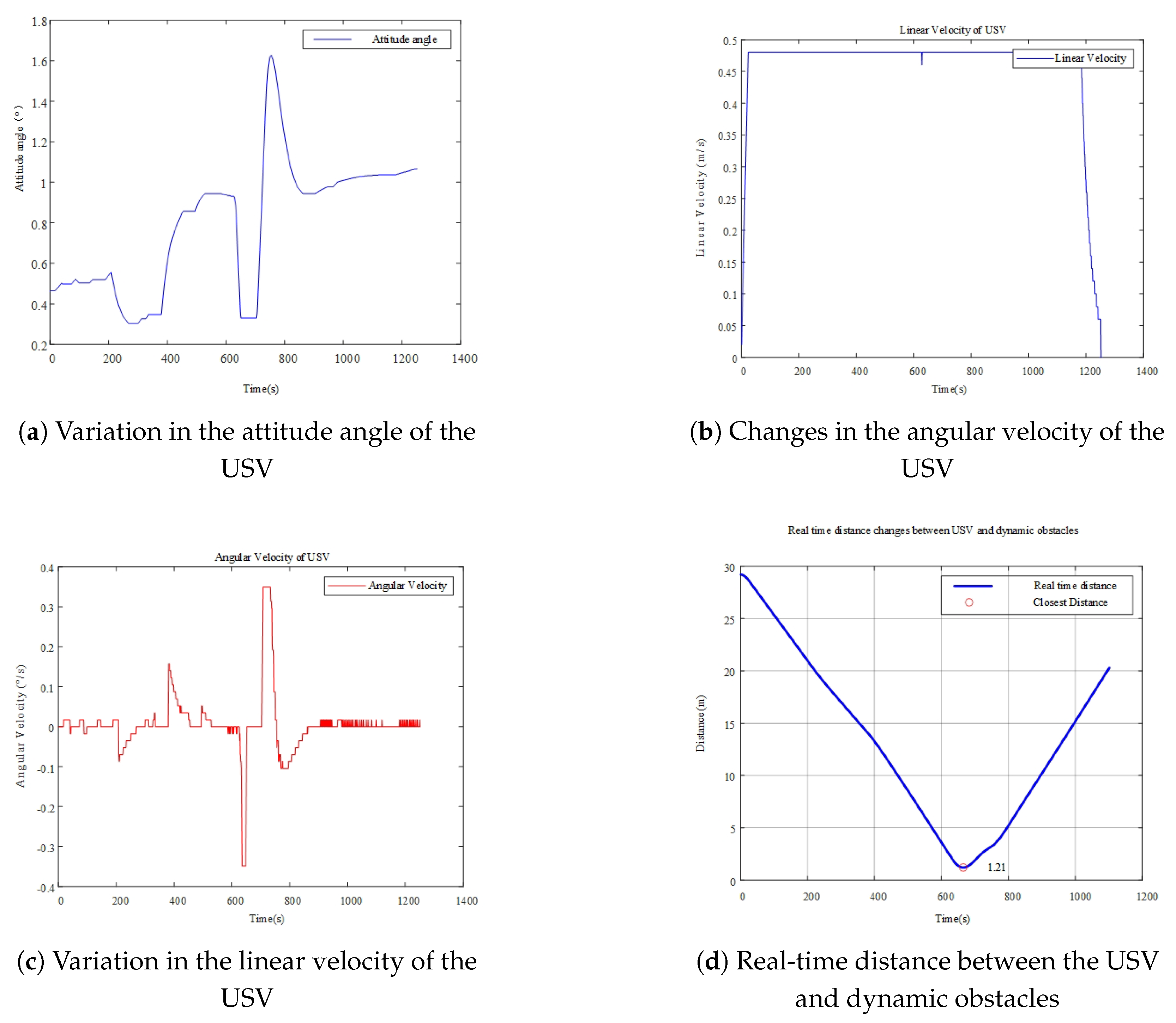
4.3. Dynamic Obstacle Avoidance

Conduct dynamic obstacle avoidance simulation experiments using the 40 × 40 map in Section 4.2. The starting point of the dynamic obstacle is set to [19,24], and the endpoint is set to [30,16]. The dynamic obstacle moves from the starting point to the endpoint at a speed of 0.01 square meters per second. The initial movement speed of the USV is 0.03 square meters per second, the maximum rotation speed is 20 °/s, and the rotation acceleration is 50 °/${\mathrm{s}}^2$. The path planning results are shown in Figure 14, and the changes in attitude angle, angular velocity, and linear velocity of the USV, as well as the real-time distance between the USV and dynamic obstacles, are shown in Figure 15.

Figure 15a presents the attitude angle variation curve of the USV during navigation. As observed, the attitude angle remains stable for most of the journey, with no abrupt changes. This stability is attributed to the path smoothing strategy, which effectively reduces unnecessary fluctuations and ensures that the USV maintains a smooth and steady posture. However, between 650 s and 700 s, a significant fluctuation occurs, indicating that the USV is actively performing dynamic obstacle avoidance maneuvers. This abrupt change is a direct result of the movement of dynamic obstacles, requiring the USV to adjust its heading dynamically to navigate safely around them. The rapid change in attitude angle during this period highlights the responsiveness of the proposed obstacle avoidance strategy.

Figure 15c further corroborates this observation by illustrating the angular velocity variations of the USV. The noticeable changes in both the direction and magnitude of the angular velocity indicate that the USV underwent significant dynamic adjustments to avoid obstacles effectively. These fluctuations demonstrate that the obstacle avoidance mechanism responds in real time to environmental changes, ensuring safe navigation without compromising the overall stability of the USV.

Figure 15b shows the variation in the linear velocity of the USV. The graph indicates that the linear velocity remains relatively stable throughout the navigation process, suggesting that the USV maintains a consistent speed under normal conditions. At the start, the linear velocity gradually increases as the USV accelerates, and towards the endpoint, it decreases steadily until reaching zero. Notably, before dynamic obstacle avoidance, a slight decrease in linear velocity is observed. This reduction occurs as the USV anticipates and prepares for obstacle avoidance by adjusting its heading. The temporary decline in linear velocity during this period ensures that the USV can maneuver safely and effectively, preventing abrupt speed changes that could destabilize its movement.

Overall, these observations confirm that the proposed path planning and obstacle avoidance strategies successfully enable the USV to navigate safely and efficiently in dynamic environments. The combination of stable attitude control, adaptive angular velocity adjustments, and smooth linear velocity variations ensures that the USV can maintain a balance between safety, efficiency, and stability throughout the navigation process.

5. Results

This paper proposes a hybrid path planning method that combines the improved A-Star algorithm with the DWA, aiming to address the limitations and safety concerns of traditional A* algorithms in global path planning, as well as their inability to perform dynamic obstacle avoidance. In Section 2, we introduce three main improvements to the A-Star algorithm: first, we optimized the search strategy to prevent the path from passing through obstacle vertices and narrow passages, thereby enhancing the safety and feasibility of the path planning process; second, we performed node optimization and path smoothing, incorporating an adaptive control point selection strategy based on Bézier curves to improve path smoothness and driving stability. In Section 3, we conducted kinematic modeling of the USV and incorporated its kinematic characteristics into the DWA, considering physical constraints such as angular velocity and linear velocity to ensure that the USV can perform obstacle avoidance in accordance with its dynamic properties.

In Section 4, we validated the effectiveness of the proposed method through simulation experiments. First, the experimental results demonstrate that the proposed algorithm achieves improvements in path length, number of nodes, and path smoothness. Second, when compared with other path planning algorithms, the proposed method shows significant advantages across various performance indicators. Finally, dynamic obstacle avoidance simulation experiments were conducted, and the results show that the USV can effectively avoid dynamic obstacles based on the global path, maintaining a safe distance from obstacles at all times to ensure navigation safety.

This study provides significant theoretical support and practical implications for the autonomous navigation and path planning of USVs. Specifically, in the domain of safe path planning within dynamic environments, the proposed method effectively enhances navigation safety, mitigates collision risks, and ensures reliable operation of a USV in complex, unpredictable settings. Although the current approach prioritizes safety optimization, future work will aim to incorporate additional performance metrics, such as energy efficiency and error indicators, into the path planning framework. These metrics are expected to further improve the system’s overall efficiency and precision, facilitating more sustainable and adaptable USV operations in real-world applications.

References

1. Liu, Z.; Zhang, Y.; Yu, X.; Yuan, C. Unmanned surface vehicles: An overview of developments and challenges. Annu. Rev. Control 2016, 41, 71–93. [Google Scholar] [CrossRef]
2. Xing, B.; Yu, M.; Liu, Z.; Tan, Y.; Sun, Y.; Li, B. A Review of Path Planning for Unmanned Surface Vehicles. J. Mar. Sci. Eng. 2023, 11, 1556. [Google Scholar] [CrossRef]
3. Hu, S.; Tian, S.; Zhao, J.; Shen, R. Path planning of an unmanned surface vessel based on the improved A-Star and dynamic window method. J. Mar. Sci. Eng. 2023, 11, 1060. [Google Scholar] [CrossRef]
4. Dijkstra, E.W. A Note on Two Problems in Connection with Graphs. Numer. Math. 1959, 1, 101–118. [Google Scholar] [CrossRef]
5. LaValle, S. Rapidly-Exploring Random Trees: A New Tool for Path Planning. In Research Report 9811; Department of Computer Science, Iowa State University: Ames, IA, USA, 1998. [Google Scholar]
6. Holland, J.H. Adaptation in Natural and Artificial Systems: An Introductory Analysis with Applications to Biology, Control, and Artificial Intelligence; MIT Press: Cambridge, MA, USA, 1992. [Google Scholar]
7. Dorigo, M.; Di Caro, G.; Gambardella, L.M. Ant algorithms for discrete optimization. Artif. Life 1999, 5, 137–172. [Google Scholar] [CrossRef] [PubMed]
8. Hart, P.E.; Nilsson, N.J.; Raphael, B. A formal basis for the heuristic determination of minimum cost paths. IEEE Trans. Syst. Sci. Cybern. 1968, 4, 100–107. [Google Scholar] [CrossRef]
9. Wang, F.; Zhao, L.; Bai, Y. Path planning for unmanned surface vehicles based on modified artificial fish swarm algorithm with local optimizer. Math. Probl. Eng. 2022, 2022, 1283374. [Google Scholar] [CrossRef]
10. Deng, F.; Jin, L.; Hou, X.; Wang, L.; Li, B.; Yang, H. COLREGs: Compliant dynamic obstacle avoidance of USVs based on the dynamic navigation ship domain. J. Mar. Sci. Eng. 2021, 9, 837. [Google Scholar] [CrossRef]
11. Zhao, J.; Wang, P.; Li, B.; Bai, C. A DDPG-Based USV Path-Planning Algorithm. Appl. Sci. 2023, 13, 10567. [Google Scholar] [CrossRef]
12. Ren, J.; Zhang, J.; Cui, Y. Autonomous obstacle avoidance algorithm for unmanned surface vehicles based on an improved velocity obstacle method. ISPRS Int. J. Geo-Inf. 2021, 10, 618. [Google Scholar] [CrossRef]
13. Wang, Y.; Li, J.; Zhao, S.; Su, P.; Fu, H.; Niu, H. Hybrid path planning for USV with kinematic constraints and COLREGS based on improved APF-RRT and DWA. Ocean Eng. 2025, 318, 120128. [Google Scholar] [CrossRef]
14. Liang, J.; Liu, L. Optimal path planning method for unmanned surface vehicles based on improved shark-inspired algorithm. J. Mar. Sci. Eng. 2023, 11, 1386. [Google Scholar] [CrossRef]
15. Gu, Y.; Rong, Z.; Tong, H.; Wang, J.; Si, Y.; Yang, S. Unmanned surface vehicle collision avoidance path planning in restricted waters using multi-objective optimisation complying with COLREGs. Sensors 2022, 22, 5796. [Google Scholar] [CrossRef]
16. Wang, D.; Chen, H.; Lao, S.; Drew, S. Efficient path planning and dynamic obstacle avoidance in edge for safe navigation of USV. IEEE Internet Things J. 2023, 11, 10084–10094. [Google Scholar] [CrossRef]
17. Jaramillo-Martínez, R.; Chavero-Navarrete, E.; Ibarra-Pérez, T. Reinforcement-Learning-Based Path Planning: A Reward Function Strategy. Appl. Sci. 2024, 14, 7654. [Google Scholar] [CrossRef]
18. Vashisth, A.; Rückin, J.; Magistri, F.; Stachniss, C.; Popovic, M. Deep Reinforcement Learning with Dynamic Graphs for Adaptive Informative Path Planning. IEEE Robot. Autom. Lett. 2024, 9, 7747–7754. [Google Scholar] [CrossRef]
19. Yang, X.; Shi, Y.; Liu, W.; Ye, H.; Zhong, W.; Xiang, Z. Global path planning algorithm based on double DQN for multi-tasks amphibious unmanned surface vehicle. Ocean Eng. 2022, 266, 112809. [Google Scholar]
20. Zhou, X.; Wu, P.; Zhang, H.; Guo, W.; Liu, Y. Learn to navigate: Cooperative path planning for unmanned surface vehicles using deep reinforcement learning. IEEE Access 2019, 7, 165262–165278. [Google Scholar] [CrossRef]
21. Zhao, Z.; Zhu, B.; Zhou, Y.; Yao, P.; Yu, J. Cooperative path planning of multiple unmanned surface vehicles for search and coverage task. Drones 2022, 7, 21. [Google Scholar] [CrossRef]
22. Zhang, M.; Yu, S.R.; Chung, K.S.; Chen, M.L.; Yuan, Z.M. Time-optimal path planning and tracking based on nonlinear model predictive control and its application on automatic berthing. Ocean Eng. 2023, 286, 115228. [Google Scholar] [CrossRef]
23. Yang, C.; Pan, J.; Wei, K.; Lu, M.; Jia, S. A novel unmanned surface vehicle path-planning algorithm based on A* and artificial potential field in ocean currents. J. Mar. Sci. Eng. 2024, 12, 285. [Google Scholar] [CrossRef]
24. Wang, Y.; Yu, X.; Liang, X. Design and Implementation of Global Path Planning System for Unmanned Surface Vehicle among Multiple Task Points. Int. J. Veh. Auton. Syst. 2018, 14, 82–105. [Google Scholar] [CrossRef]
25. Tiwari, A.K.; Nadimpalli, S.V. New Fusion Algorithm Provides an Alternative Approach to Robotic Path Planning. arXiv 2020, arXiv:2006.05241. [Google Scholar]
26. Kabir, R.; Watanobe, Y.; Islam, M.R.; Naruse, K. Enhanced Robot Motion Block of A-star Algorithm for Robotic Path Planning. Sensors 2024, 24, 1422. [Google Scholar] [CrossRef]
27. Hu, Y.; Harabor, D.; Qin, L.; Yin, Q. Regarding goal bounding and jump point search. J. Artif. Intell. Res. 2021, 70, 631–681. [Google Scholar] [CrossRef]
28. Zhang, J.; Ling, H.; Tang, Z.; Song, W.; Lu, A. Path planning of USV in confined waters based on improved A* and DWA fusion algorithm. Ocean Eng. 2025, 322, 120475. [Google Scholar] [CrossRef]
29. Han, X.; Zhang, X. Multi-scale ThetA* algorithm for the path planning of unmanned surface vehicle. Proc. Inst. Mech. Eng. Part M J. Eng. Marit. Environ. 2022, 236, 427–435. [Google Scholar] [CrossRef]
30. Han, S.; Wang, L.; Wang, Y.; He, H. A dynamically hybrid path planning for unmanned surface vehicles based on non-uniform Theta* and improved dynamic windows approach. Ocean Eng. 2022, 257, 111655. [Google Scholar] [CrossRef]
31. Wang, Z.; Liang, Y.; Gong, C.; Zhou, Y.; Zeng, C.; Zhu, S. Improved dynamic window approach for Unmanned Surface Vehicles’ local path planning considering the impact of environmental factors. Sensors 2022, 22, 5181. [Google Scholar] [CrossRef]
32. Xu, D.; Yang, J.; Zhou, X.; Xu, H. Hybrid path planning method for USV using bidirectional A* and improved DWA considering the manoeuvrability and COLREGs. Ocean Eng. 2024, 298, 117210. [Google Scholar] [CrossRef]
33. Yao, M.; Deng, H.; Feng, X.; Li, P.; Li, Y.; Liu, H. Global Path Planning for Differential Drive Mobile Robots Based on Improved BSGA* Algorithm. Appl. Sci. 2023, 13, 11290. [Google Scholar] [CrossRef]
34. Liu, L.; Wang, B.; Xu, H. Research on path-planning algorithm integrating optimization A-star algorithm and artificial potential field method. Electronics 2022, 11, 3660. [Google Scholar] [CrossRef]
35. Hassani, V.; Lande, S.V. Path planning for marine vehicles using Bézier curves. IFAC-PapersOnLine 2018, 51, 305–310. [Google Scholar] [CrossRef]
36. Lai, R.; Wu, Z.; Liu, X.; Zeng, N. Fusion algorithm of the improved A* algorithm and segmented bezier curves for the path planning of mobile robots. Sustainability 2023, 15, 2483. [Google Scholar] [CrossRef]
37. Yin, X.; Cai, P.; Zhao, K.; Zhang, Y.; Zhou, Q.; Yao, D. Dynamic path planning of AGV based on kinematical constraint A* algorithm and following DWA fusion algorithms. Sensors 2023, 23, 4102. [Google Scholar] [CrossRef]
Figure 1. (a) Schematic diagram of 4-neighborhood search. (b) 8-neighborhood search diagram.
Jmse 13 00934 g001
Figure 2. Path planning diagram of heuristic functions at different distances: (a) Manhattan distance. (b) Euclidean distance. (c) Chebyshev distance.
Jmse 13 00934 g002
Figure 3. The situation where a USV passes through the vertex of an obstacle or a narrow passage between two obstacles.
Jmse 13 00934 g003
Figure 4. Schematic diagram of node search strategy improvement: (a) Definition of hazardous nodes. (b) Path selection when obstacles are separated by a node. (c) Path selection when obstacles are separated by two nodes.
Jmse 13 00934 g004
Figure 5. Traditional A-Star algorithm path planning result chart and improved A-Star algorithm path planning result chart: (a) Traditional A-Star algorithm. (b) Improve the A-Star algorithm.
Jmse 13 00934 g005
Figure 6. Comparison chart of the effect before and after initial processing of nodes: (a) Before processing. (b) After processing.
Jmse 13 00934 g006
Figure 7. Node further processing annotation graph: (a) Node connection crossing obstacles. (b) Parallel lines connecting nodes.
Jmse 13 00934 g007
Figure 8. Comparison results of node optimization strategy simulation: (a) Traditional A* algorithm path planning diagram. (b) Path planning diagram after node optimization.
Jmse 13 00934 g008
Figure 9. Schematic diagram for selecting control points of a Bézier curve.
Jmse 13 00934 g009
Figure 10. Schematic diagram of the three-degree-of-freedom motion model for unmanned boats.
Jmse 13 00934 g010
Figure 11. Block diagram of the control system.
Jmse 13 00934 g011
Figure 12. Simulation results of various improved path planning in global path planning.
Jmse 13 00934 g012
Figure 13. Comparison of different algorithm path planning.
Jmse 13 00934 g013
Figure 14. Dynamic obstacle avoidance path planning result diagram.
Jmse 13 00934 g014
Figure 15. Variation in the attitude angle, velocities, and distance to obstacles of the USV.
Jmse 13 00934 g015