Abstract
Reinforcement learning has made significant progress in single-agent applications, but it still faces various challenges in multi-agent scenarios. This study investigates the application of reinforcement learning algorithms in a competitive game scenario of multi-autonomous underwater vehicle (multi-AUV) hunting the evaders. We introduce an optimality operator and redefine the objective function of multi-agent reinforcement learning (MARL), transforming the uncertain states of other agents into solvable inference problems, namely the Regularized Competitor Model (RCM). Leveraging RCM, multi-agent systems can optimize strategies in competitive game training more efficiently. We verify and analyze the performance of the proposed algorithm in a multi-AUV hunting scenario. Simulation results demonstrate that the proposed algorithm exhibits strong adaptability and a higher success rate than the baseline in hunting the evaders.
1. Introduction
Deep Reinforcement Learning (DRL) allows agents to have independent exploration and learning capabilities, which enable them to interact continuously with the environment and enhance their behavior through trial and error [1]. Leveraging this, DRL algorithms can assist multiple Autonomous Underwater Vehicles (AUVs) in making independent decisions in complex underwater environments. AUVs are capable of learning optimal behavioral strategies to accomplish specific tasks, such as searching [2,3], tracking [4,5,6], detecting [7], or hunting [8,9]. This ability allows AUVs to make intelligent decisions based on the current context without the need for strict manual control [10]. Given the dynamic nature of underwater environments, DRL algorithms contribute to improving the efficiency of multi-AUV systems by optimizing resource utilization, reducing energy consumption, and shortening task completion time, thereby enhancing overall performance [11].
Unfortunately, traditional reinforcement learning approaches such as Q-Learning or policy gradient are poorly suited to multi-agent environments [12]. One major challenge is that the strategy of each agent evolves during training, making the environment non-stationary from the perspective of any individual agent [13]. This poses learning stability challenges and prevents the direct use of past experience replay [14]. The presence of multiple agents introduces additional uncertainty to the environment. Therefore, the capability to deduce the characteristics of other agents, such as beliefs, private information, behaviors, and strategies, is crucial [15]. Moreover, the actual operational environment of AUVs is inherently complex and poses higher risks. Consequently, it is necessary to perform pre-training to ensure the adaptability and effectiveness of AUVs in challenging conditions. The diversity of the pre-training environment significantly impacts the overall performance of the trained policies [16].
To address these challenges and difficulties, researchers have proposed numerous Multi-Agent Reinforcement Learning (MARL) algorithms. Rashid et al. [17] proposed the QMIX method, which employs a hybrid network to estimate joint action-values as a monotonic combination of per-agent values. By leveraging a hybrid network to combine single-agent local value functions and incorporating global state information during training, the performance of the algorithm is improved. Additionally, this ensures consistency between centralized and decentralized policies. MADDPG [14], an extension of the DDPG algorithm proposed by OpenAI, adopts a centralized training and decentralized execution approach. Its structure mirrors that of DDPG, with each agent utilizing an independent actor network to observe state outputs and determine actions. However, it faces challenges in large-scale MARL with numerous agents due to the need to train separate actor networks for each agent, which potentially leads to increased computational burden and suboptimal performance. Foerster et al. [18] proposed a Bayesian Action Decoder (BAD) in 2019. BAD uses neural networks to allow each agent to infer information about their teammates. To avoid infinite recursive thinking, a public belief system is established by the system [19], which represents all publicly available information about the game state, previous actions, and inferred perspectives of other agents without direct observation. Each agent takes action based on their own observations under the guidance of public belief. Throughout the process, the action space consists of deterministic local strategies that can be sampled for a given common state. In multi-agent training methods, inference related to other agents generally involves strategic interactions among intelligent agents.
Opponent modeling has recently emerged as a crucial component within MARL, enabling agents to effectively anticipate and adapt to the behaviors of other learning agents. Recent studies have framed opponent modeling as a probabilistic inference problem. Wen et al. [20] introduced Probabilistic Recursive Reasoning (PR2), which models each agent’s policy as a conditional distribution, recursively considering the potential future actions of other agents. Another significant contribution is ROMMEO (Regularized Opponent Model with Maximum Entropy Objective) [15], which introduces regularization based on maximum entropy principles to stabilize the learning process and jointly optimize both the agent’s policy and its beliefs about opponents. Additionally, Davies [21] proposed Learning to Model Opponent Learning (LeMOL), which develops a structured model of opponents’ learning dynamics. This structured opponent model is shown to be more accurate and stable than naive behavior cloning baselines and can enhance the performance of algorithmic agents in multi-agent settings.
Game-theoretic approaches facilitate decision-making and strategic interactions across multiple application domains by considering model complexity, decision support capabilities, and employing strategy analysis tools. In the context of MARL, competitive games that incorporate multiple factors, such as the number of participants and the diversity of strategies, facilitate the analysis of the consequences and potential outcomes associated with different strategic choices [22]. This enhances the understanding of the complexity and uncertainty inherent in real-world scenarios, thereby assisting decision-makers in formulating strategies and counterstrategies.
This paper combines game training methods with MARL, and proposes a Regularized Competitor Model-based Algorithm (RCM) to enhance the performance of multi-AUV systems in hunting tasks. The main contributions are as follows:
- (i)
- Integrating the Competitor Model into the Objective Function. By introducing a binary stochastic variable, denoted as ‘optimality’ (o), this study transforms the strategy modeling of a single agent interacting with other agents into a probabilistic inference problem. The likelihood variational lower bound for achieving optimality is derived as a new objective function for MARL, while the strategies of competitors are modeled using a regularization approach. The competitor model can more accurately learn the strategies of other agents, improve the training efficiency of MARL, and achieve faster convergence.
- (ii)
- Training within a Competitive Game Framework. When converging to a Nash equilibrium, each intelligent agent selects its optimal strategy given a fixed competitor strategy to maximize its own gains. Applying the same reinforcement learning model to both competing sides enables diverse simulation experiments and improves the generalization ability of training.
The rest of this paper is organized as follows: Section 2 introduces the proposed algorithm framework and outlines the basic model and concepts. It incorporates the competitor model into MARL, enabling the inference of other agents’ strategies by optimizing an optimality variable. This leads to the proposal of a Maximum Entropy Reinforcement Learning Algorithm based on Regularized Competitor Model (RCMAC). Section 3 presents a case study on the application of the algorithm in an underwater multi-AUV hunting scenario involving intelligent evaders. Specific configurations for state, action, and reward functions for this scenario are outlined. Section 4 demonstrates the performance of the algorithm in various hunting scenarios and evaluates RCMAC. Finally, Section 5 presents the conclusions.
2. Maximum Entropy Reinforcement Learning Algorithm Based on Regularized Competitor Model
2.1. The Proposed Framework
This study adopts the centralized training and decentralized execution (CTDE) framework similar to MADDPG. Thus, policies may utilize additional information to simplify training, provided such information is not used during testing. This approach is unsuitable for Q-learning since the Q-function typically cannot incorporate different information between training and testing. Consequently, distinct from MADDPG, a competitor model is introduced to explicitly learn additional information about other agents’ strategies during both training and testing.
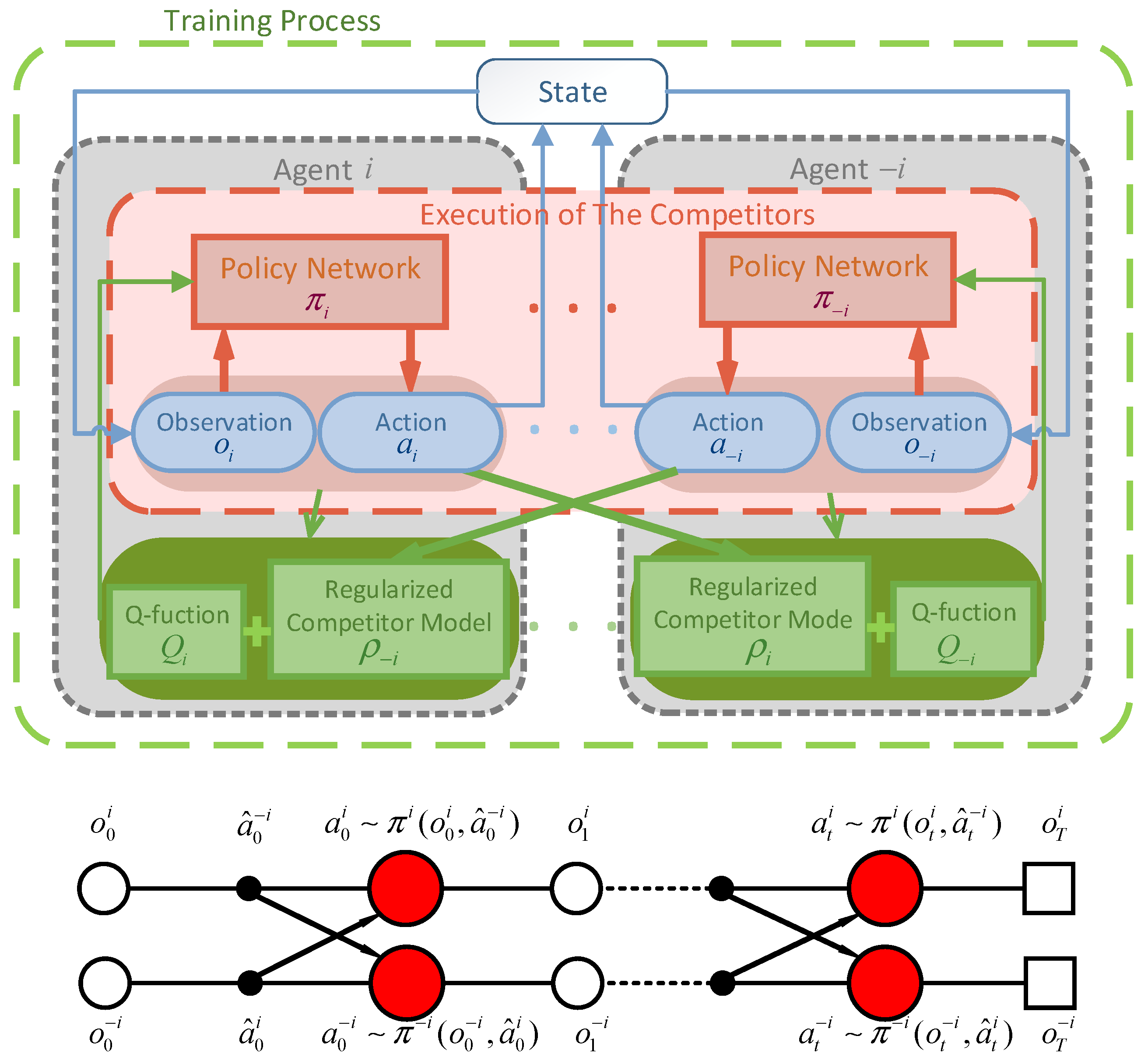
As shown in Figure 1, within the CTDE framework, the observation restricts the learned policies to use only local information during execution (i.e., their own observation data). The policy network of agent makes decisions based on its own observations, and the improved critic target function comprises two parts. During training, it can optimize the information from other agents. Here, , similar to conventional methods, is used to evaluate the action-state value of the agent itself in the current multi-agent scenario, while is used to quantify the impact of other agents’ current optimal policies on the agent itself. Figure 1 illustrates the process of distributed execution for each intelligent agent within the framework. It is important to note that the policy network relies not only on the current observation state of the agent but also makes decisions based on competitor actions inferred through the competitor model. This iterative process is followed to complete the planning strategy for each agent.
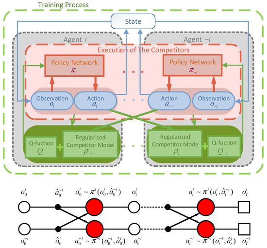
Figure 1.
The framework of the proposed algorithm.
2.2. Competitive Games
For the n-agent competitive game, a tuple is defined, where represents the state space, denotes the initial state distribution, and refers to the discount factor, For each agent , the action set and reward function are given by , respectively. The state transitions are given by the transition function , where is the combined action space.
Agent selects an action based on its policy , which is parameterized by given the state . We define the joint policy across all agents as , with representing the joint parameters. For convenience, this joint policy can be viewed from agent ’s perspective as , where , and denotes the joint policy of all agents other than . In each step of the game, agents choose their actions simultaneously. The goal of each agent is assumed to maximize its expected cumulative reward, formulated as
with sample from . For fully cooperative scenarios, it is presumed that at least one joint policy exists, enabling all agents to attain the highest possible cumulative reward together.
2.3. Regularized Competitor Model
By introducing a binary random variable , which signifies the “optimality” of agent at time , we convert the decision-making process into an inference task. In single-agent scenarios, the reward has a finite bound, but the exact probability of achieving the highest reward for a given action remains uncertain. Hence, can be viewed as a stochastic variable, and its probability distribution can be described as , satisfying . According to this equation, higher rewards imply greater probabilities of optimality (). However, the concept of “optimality” in multi-agent settings differs slightly from its interpretation in single-agent problems.
Here, we define the symbol as a general representation of an objective function. denotes the objective function of the variable with respect to parameter . In particular, without subscripts refers to the general form of the reinforcement learning objective; that is, the maximization of expected cumulative rewards.
In the context of cooperative–competitive games, the optimal solution is achieved when all intelligent agents act according to their optimal strategies, namely obtaining the maximum rewards. Thus, assuming that other agents are following their optimal strategies (i.e.,=1), the probability of the likelihood of intelligent agent also adheres to its optimal strategy and, consequently, obtains the maximum reward.
Since optimal strategies and environmental models are presumed unknown beforehand, they are considered as latent variables. To optimize the samples observed as defined in Equation (3), following the derivations in reference [23,24,25,26,27], we employ the method of Variational Inference (VI). These latent variables are represented by an auxiliary distribution, denoted as . By decomposing the above expression according to the modeling assumptions, we obtain
In this decomposition, a lower bound on the probability density of the optimality for the intelligent agent can be obtained by utilizing the initial state and state transition probabilities as the prior distribution
where represents the competitor model for intelligent agent and is used to estimate the optimal strategy of its competitor. is the conditional strategy of agent under optimal conditions . denotes the prior probability of the competitor’s optimal strategy. The prior is set as an empirical distribution of competitor actions in a given state. Since the optimization of the objective function is only concerned with the case , this term can be eliminated from . Equation (5) provides a variational lower bound on .
Equation (5) can be expanded further into Equation (6), where the first portion corresponds to the maximum entropy formulation used in the SAC algorithm. It is necessary to clarify which component is associated with reward maximization and which relates to entropy maximization, along with a comparative discussion relative to the SAC formulation. For agent , we enhance the standard expected reward by adding the entropy term of its conditional policy, . This combined expression serves as the Maximum Entropy Objective (MEO) for agent . It should be emphasized that optimizing the MEO simultaneously contributes to optimizing the competitor model .
2.4. Regularized Competitor Model with Maximum Entropy Objective Actor-Critic (RCMAC)
In this section, we propose an extension of the Soft Q-iteration algorithm [23] to multi-agent scenarios. Although our derivation follows a similar reasoning as that presented in reference [23], generalizing Soft Q-learning to a MARL context introduces additional complexity. To accommodate this, we slightly adjust the objective presented in Equation (6) by introducing an entropy weighting factor, . Setting recovers the original objective formulation.
The multi-agent soft Q-function and V-function are defined, respectively, as below. The conditional policies and competitor models defined in Equations (9) and (10) are the optimal solutions with respect to the objectives defined in Equation (6):
The soft state-action value function of agent is
and the soft state value function is
Then, the optimal conditional policy and competitor models for Equation (6) are
and
Similar to the derivation of gradient updates in SAC, we define parameterized Q-networks, conditional policy networks, and competitor models as follows: . Here, the trainable parameters are , , and with the objective of minimizing the target function:
where
Adopting the update mechanism of the twin Q-networks, represents the target action-value function to ensure a relatively stable target value. denotes the action sampled from the competitor model of intelligent agent , . It is essential to distinguish this from the actual action taken by the competitor .
Solving the optimal conditional policy and competitor models in Equations (9) and (10) has proven to be challenging in complex unknown environments. Following the approach outlined in reference [24], we constructed an objective function and train parameters and to minimize the KL divergence:
where , , therefore and can be derived as
The gradients of are
3. Multi-AUV Hunting with RCMAC
3.1. Environmental State Description
3.1.1. AUV Motion Model
To facilitate the description of the state and action of an AUV, this section initially presents the motion model of the AUV. It is assumed that the underactuated AUV is controlled by horizontal thrusters, fore and aft symmetrical vertical thrusters, and vertical rudders in a 3-dimensional underwater environment.
Figure 2 illustrates that represent the heeling angle, trim angle, and slant angle within the AUV’s inertial coordinate system (positive values indicate counterclockwise rotation). The velocity components of the AUV in the carrier coordinate frame are denoted by . Additionally, represent the angular velocity components in the same carrier coordinate frame. Typically, the AUV’s state is described using six degrees of freedom within the inertial coordinate system, represented as the vector [28]. To simplify calculations, this study assumes a simplified AUV model with vertical thrusters enabling movement along the Z-axis. Since lateral shifts and rolling movements are generally restricted under normal operational conditions, the inertial coordinate system’s attitude reduces to .
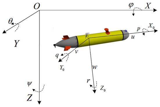
Figure 2.
AUV motion model.
Furthermore, the AUV’s motion within the carrier coordinate frame is represented using the velocity vector . Here, indicates the angle between the forward velocity component and the X-axis, denotes vertical velocity along the Z-axis, and corresponds to the rate of change of (). Therefore, the simplified motion model for the AUV can be described as follows:
The velocity change of the AUV is defined as the action, and represented as
Based on the above formulas, the self-state of the AUV can be described by , and expressed as
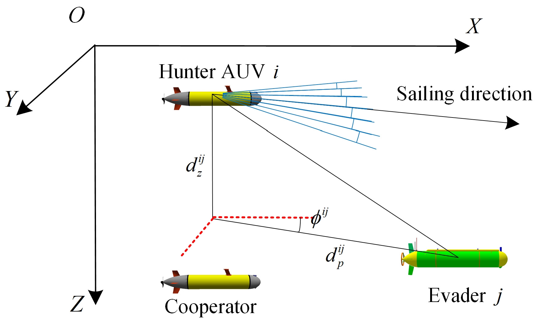
3.1.2. State of the Competitors (Including Cooperators and the Evader)
The position information of cooperators and evader is necessary for the AUV group to encircle the evader [29]. As shown in Figure 3, the relative positions of the cooperating agents and the evader in a three-dimensional environment are indicated by the coordinates . vectors extend from the current location of the AUV toward competitor (either cooperators or the evader). Where, denotes the projected length of vector onto the horizontal (XOY) plane, represents the angle formed between vector and the positive X-axis, and specifies the vertical projection length along the Z-axis. Consequently, the relative state between the AUV, its cooperators, and the evader can be expressed by the following equation:
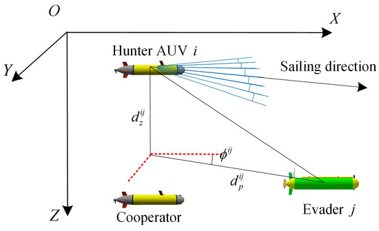
Figure 3.
The description of the competitors (The red dashed lines indicate the projections onto the coordinate axes).
During the training process of the reinforcement learning algorithm, the state of each AUV is comprised of the pose and the relative positions with respect to the competitors. Therefore, can be described as .
3.2. Criteria for a Successful Hunting Progress
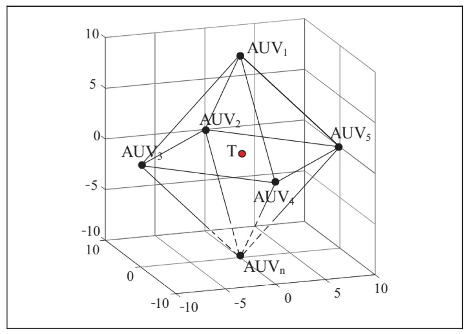
In the hunting scenario presented in this paper, a group of AUVs are tasked with hunting an intelligent evader. Assuming there are n AUVs (AUV1, AUV2, …, AUVn), and each AUV is equipped with a special device capable of disrupting the mobility of the evader. It is assumed that the mobility of the evader will be restricted when any hunting AUV successfully approaches it within a range of 1 m. The process of hunting involves the movement of hunting AUVs towards the evader within the hunting cluster. The hunting AUVs need to surround the evader as closely as possible and evenly distribute around them around the evader to restrict their escape direction. At least one hunting AUV attempting to approach the evader to limit its mobility is considered a successful hunting progress.
The multi-AUV hunting of an evader in a three-dimensional underwater environment is depicted in Figure 4. AUV1 to AUVn represent the hunting target points within the encircling circle range, and T denotes the evader. The success of the hunting primarily relies on the following three criteria:

Figure 4.
The illustration of multiple AUV hunting.
- The distance between the center of the hunting formation and the evader is less than a threshold (5 m);
- The distance between the hunting AUVs and the evader is less than a threshold (10 m);
- There exists at least one hunting AUV with a distance of less than 1 m from the evader.
3.3. Reward Functions of the Hunters
For effective multi-AUV hunting, it is essential to maintain a specific formation so the AUVs can cooperatively surround the evader from multiple directions. Additionally, since the evader will actively try to break through the encirclement, the navigation goals for the AUVs must be updated continuously in response. Considering these complexities, establishing a suitable reward function is critical. In this section, we propose a continuous and modular reward function to enhance the efficiency of training. The reward structure is organized into the following three categories, corresponding to various scenarios encountered during the hunting process.
3.3.1. Cooperating Rewards
To effectively utilize cooperation among AUVs during target detection and pursuit initiation, it is important for the vehicles to maintain a suitable surrounding formation. Ideally, the distance between each AUV and the centroid of the group should remain within a controlled range, and a safe minimum separation must be maintained among individual vehicles to prevent collisions.
The cooperating reward function is therefore defined as follows:
where denotes the distance between each hunter and the geometric center of the hunter group, while represents the set of distances between each hunter and the other hunters.
3.3.2. Hunting Rewards
During the training phase, it is assumed that when an AUV detects an evader, it alerts the other hunters, prompting the entire team to initiate pursuit. Hunters are thus motivated to track and move closer to the evader. Additionally, we account for scenarios where the overall group moves closer, but an individual hunter drifts further from the evader. Under such circumstances, the respective AUV receives a positive reward to guide its actions toward fulfilling the group’s collective goal.
where denotes the distance between each hunter and the evader, while represents he distance between the evader and the geometric center of the hunter group.
3.3.3. Finishing Rewards
An episode terminates under three possible scenarios: (a) any AUV reaches the maximum allowed number of steps for its mission, (b) collision between two or more AUVs, or (c) successful encirclement of the evader by hunter AUVs, effectively restricting its potential escape routes. In each of these scenarios, the hunters receive a final reward , which signals the end of the current episode. The final rewards are specifically defined as follows:
Each AUV receives total rewards based on the following factors:
3.4. Reward Functions of the Evader
In the hunting–evading game scenario presented in this study, the evader’s action and state spaces are configured to be consistent with those of the hunters, and the evader employs the same algorithmic architecture. The key difference lies in the reward function designed for the evader. Specifically, a target point located outside the designated area is assigned to the evader to guide its escape direction. The evader receives rewards when approaching this target point and successfully exiting the boundary of the scene. Moreover, the hunting–evading interaction is formulated as a zero-sum game, meaning that from the evader’s perspective, it additionally receives a reward signal opposite to that of the hunters’ reward. These rewards are defined as follows:
where refers to the distance between the evader and the target point.
3.5. Competitive Training Process
The training process of RCMAC employs a centralized training with a distributed execution approach following the procedure below.
Initialize the replay pool and neural network parameters for all AUVs, including the joint policy network , competitor model network , and Q-network .
Repeat the following steps until convergence or the maximum iteration count is reached: (a) Each agent predicts the optimal actions of competitors based on the current competitor model. (b) Each agent calculates and selects actions based on the local observations of current state (excluding competitor states) and the competitor actions. (c) All AUVs compute the global environmental state and rewards after executing actions. (d) Each AUV updates the actual competitor actions and stores them in the experience replay buffer. (e) Each AUV samples competitor action samples from the replay pool and updates the competitor model. (f) Calculate target Q-value using the target network, and update the local and target Q-network parameters, as well as the policy network parameters for each agent. Algorithm 1 provides a step-by-step overview of the training process described above.
| Algorithm 1 RCMAC in Multi-AUV Hunting |
|
4. Simulation Results
In this section, multiple unbalanced game scenarios are demonstrated to validate the efficacy of the proposed algorithm. Comparisons with the MADDPG algorithm are also presented to showcase the superiority of the proposed algorithm.
4.1. Experimental Environment and Training Parameters
The RCMAC algorithm was implemented on a training workstation equipped with an Intel Core i9 11900K processor (8 cores, 5.1 GHz, Intel Corporation, Santa Clara, CA, USA) and a GPU with 24 GB memory (RTX 3090, NVIDIA Corporation, Santa Clara, CA, USA). The deep neural network models were built using Pytorch (Version 1.13.0) and trained using GPU acceleration. Initially, the RCMAC hyperparameters were set based on reference [15], while the parameters for Maximum Entropy Reinforcement Learning in the hunting scenario mainly followed those outlined in our earlier study [29]. Table 1 summarizes the hyperparameter settings.

Table 1.
Hyperparameters of RCMAC.
4.2. Performance and Analysis
To demonstrate the performance of the proposed algorithm in the pursuit–evasion competitive game, there are three scenarios including 1, 4, and 6 hunters hunting a single evader, respectively. denotes the initial position of the hunters and the evader. In each scenario, the evader starts from the initial position and sails towards outer boundary to escape from the hunting area.
4.2.1. Scenario A: One Hunter–One Evader Game
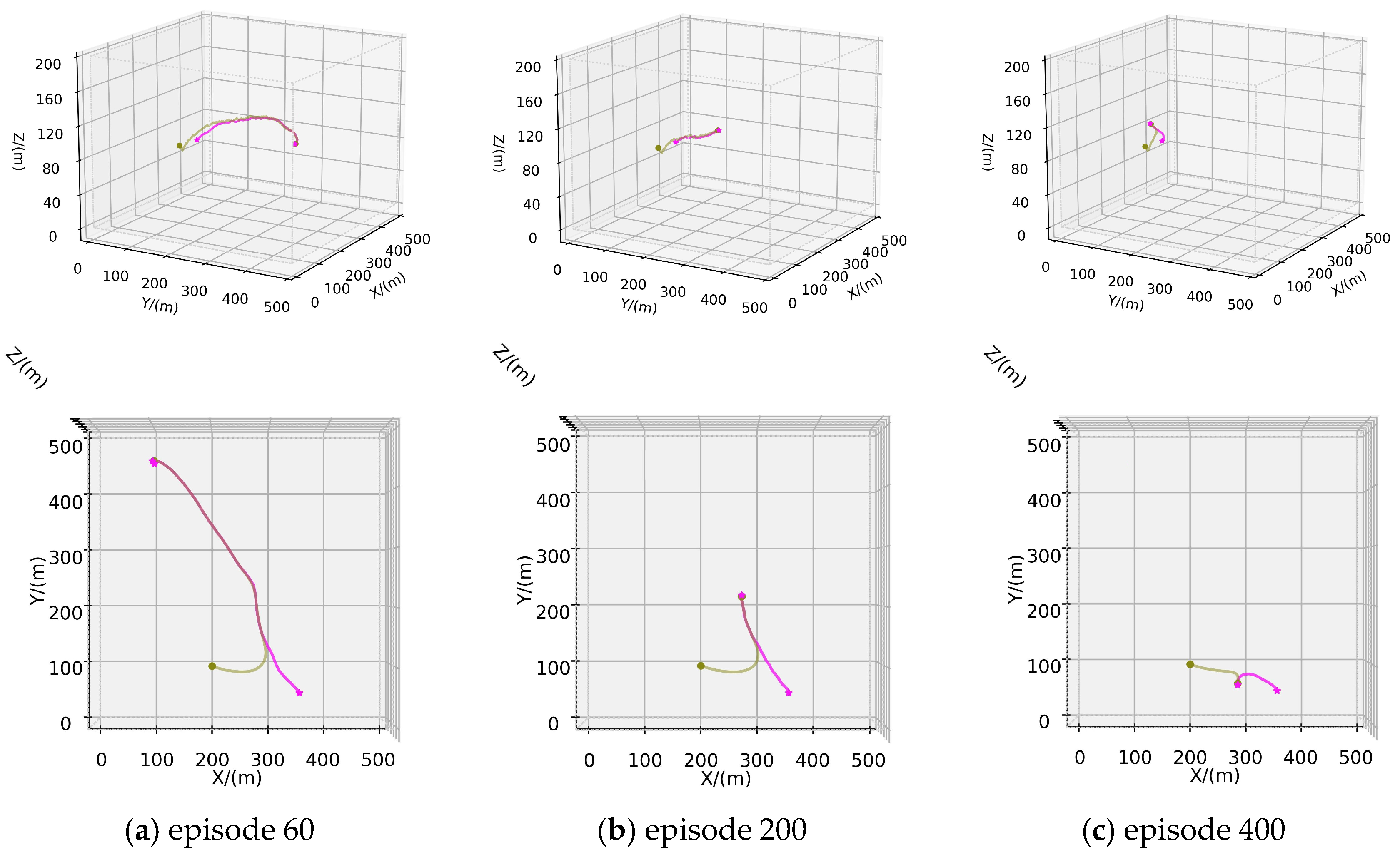
In scenario A, only one hunter is deployed to pursue the evader. The maximum speeds of the hunter and the evader are 2.7 m/s and 2.5 m/s, respectively. The initial position of the AUV is . Following the definition of successful hunting mentioned in Section 3.2, the hunter needs to chase the evader, and the hunting is deemed successful when its distance from the evader is less than 1 m. In the test scenario spanning 500 episodes, the trajectories of the hunter and the evader are depicted in Figure 5, where the pink line represents the trajectory of the evader, and the green line indicate the trajectories of the hunter.
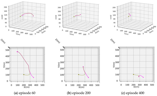
Figure 5.
Training process of Scenario A: (a) Trajectories of episode 60; (b) Trajectories of episode 200; (c) Trajectories of episode 400.
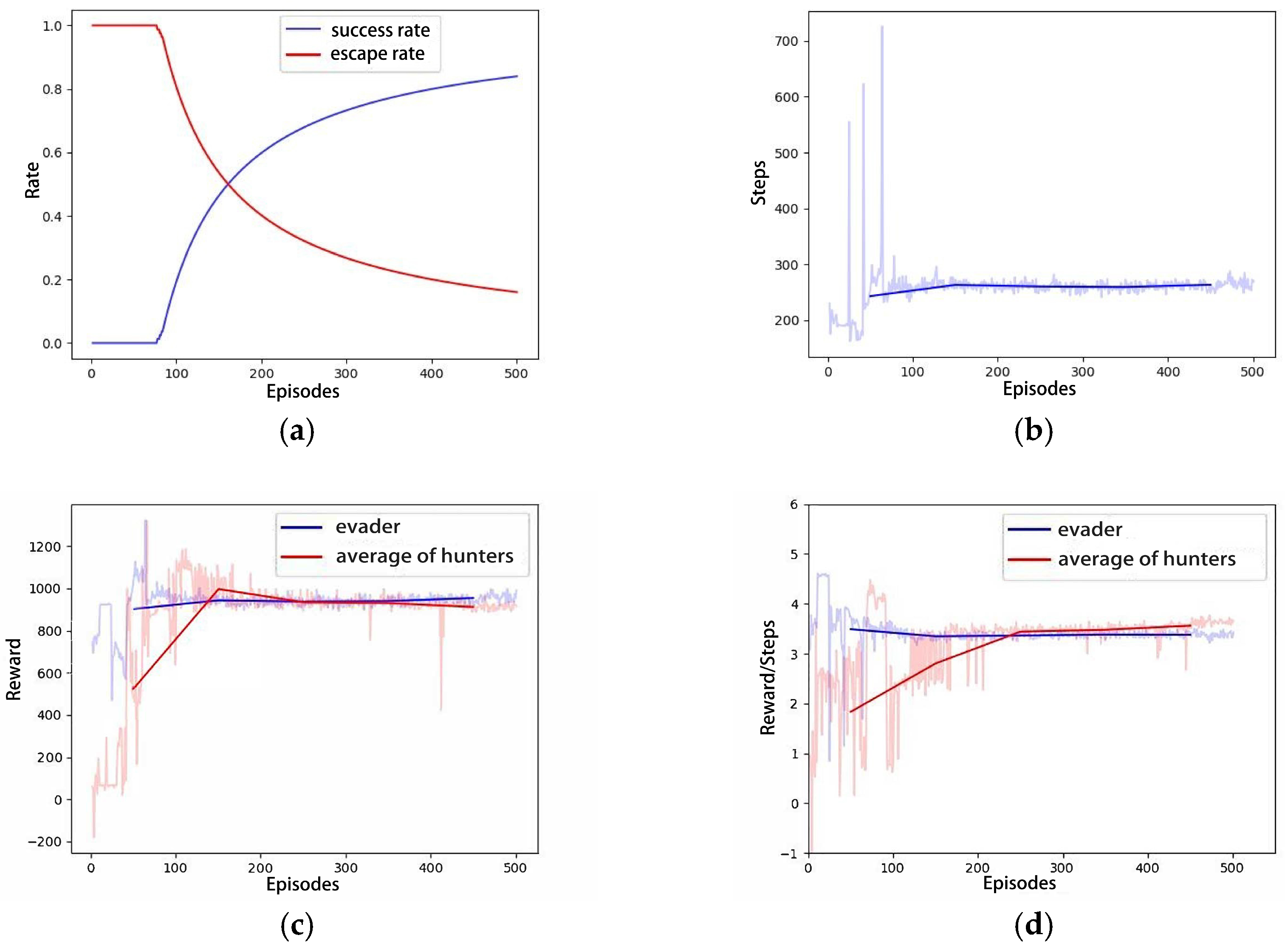
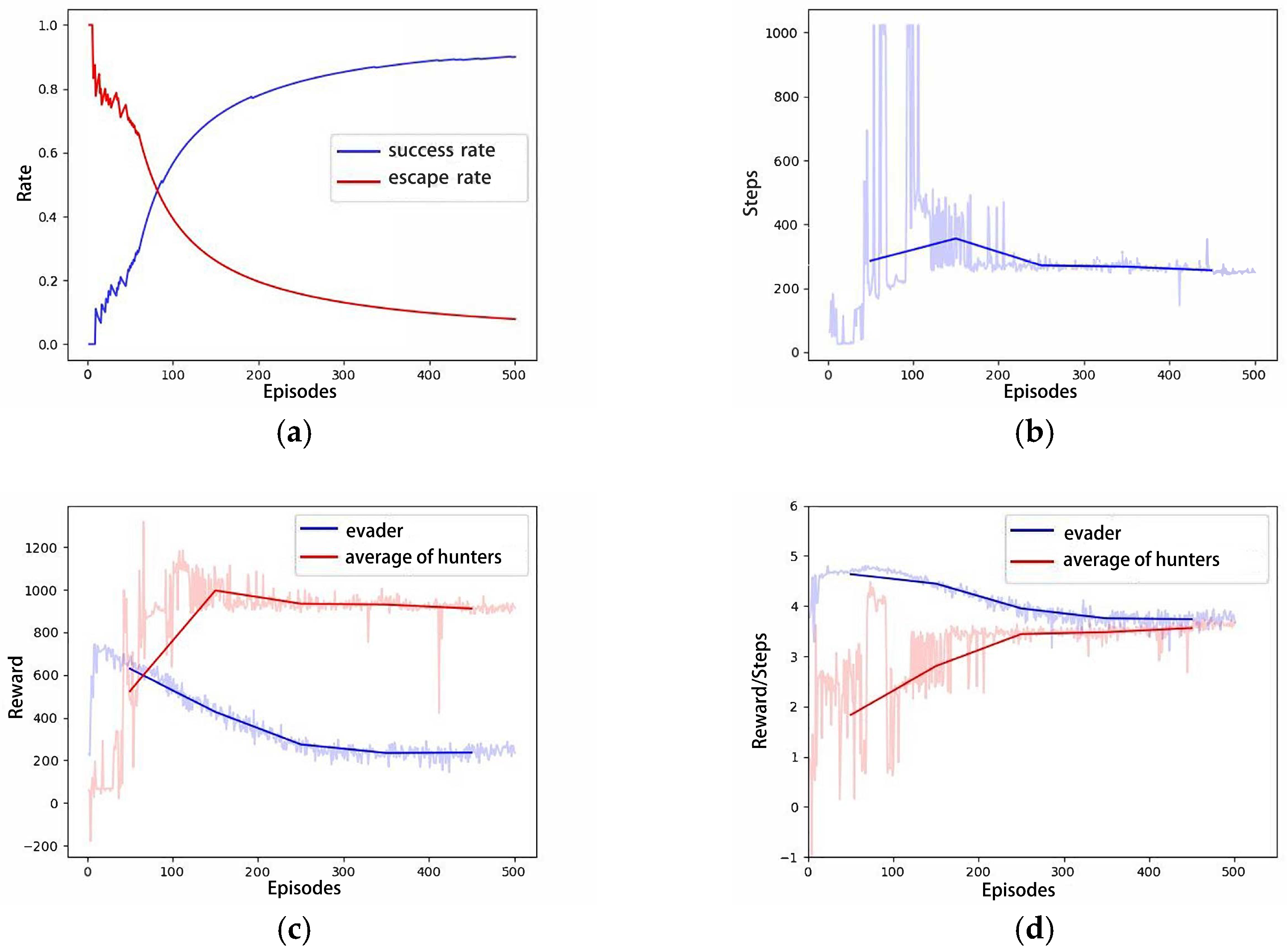
Figure 5a illustrates the trajectory of the hunter’s first successful hunting within the 500-episode experimental scenario, approaching the evader within a range of 1 m. The evader is observed to be hunted as it nears the designated escape boundary, with relatively long pursuit and evasion paths. As the training iterations increase, the pursuit and evasion paths gradually shorten, and the time required for successful hunting decreases, as depicted in Figure 5b,c. The increase in training iterations leads the competitive game training process toward a strategic equilibrium between the pursuer and the evader. The inherent speed advantage of the hunter has been demonstrated to facilitate earlier successful capture of the evader. Figure 6 illustrates the relevant curves of this process, where Figure 6a shows the cumulative hunting success rate and escape success rate for both the hunter and the evader as the number of training iterations increases. Figure 6b–d, respectively, show the conclusion steps, total rewards per episode, and the average rewards per step for both the hunter and the evader. These curves demonstrate that with the progression of the adversarial training, the hunter gradually finds shorter paths to hunt the evader, maximizing the potential for higher rewards.
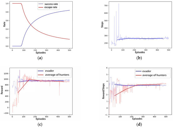
Figure 6.
The curves of Scenario A: (a) Success rate; (b) Steps; (c) Total Rewards; (d) Average Rewards per step.
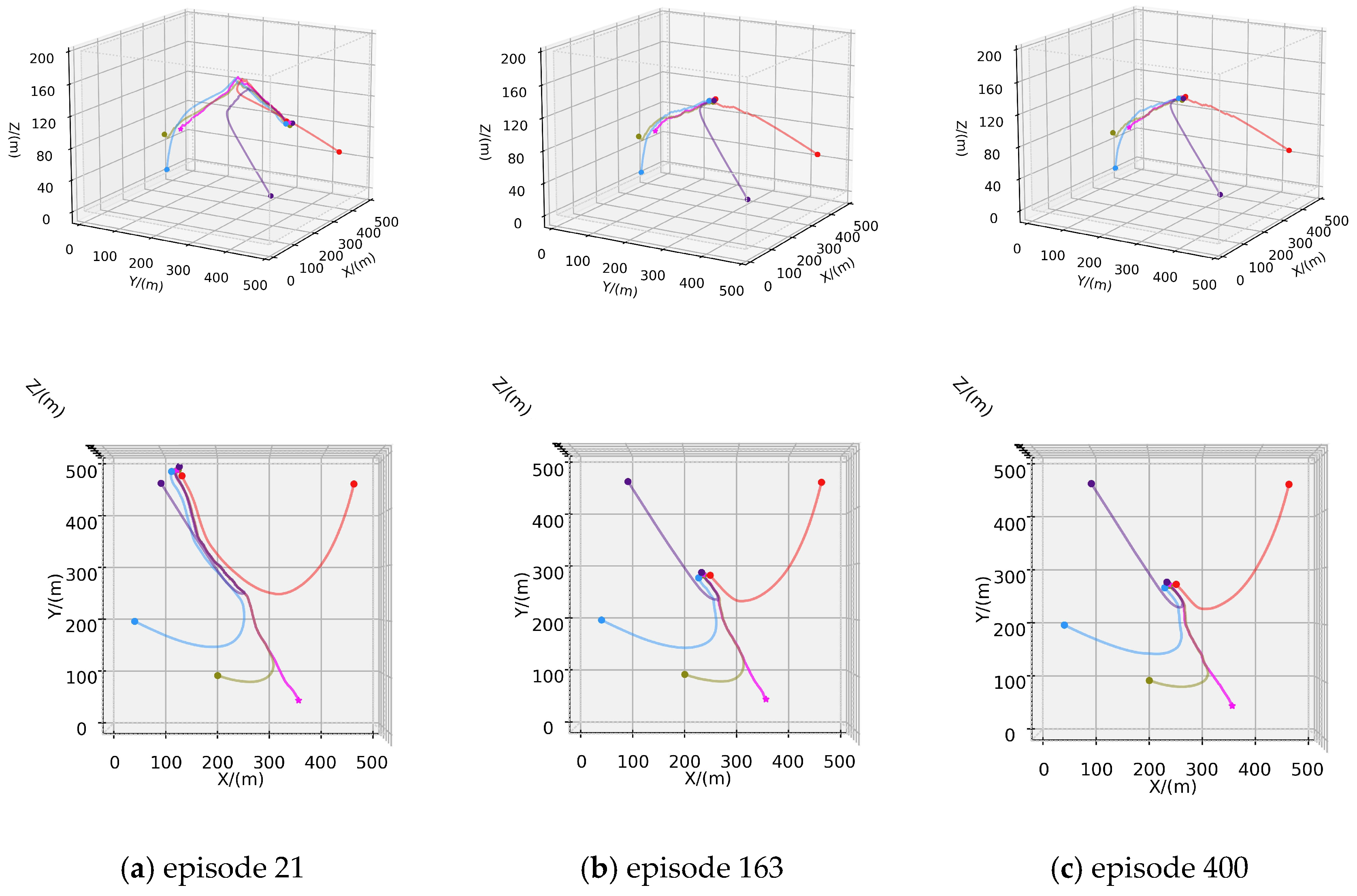
4.2.2. Scenario B: Four Hunters–One Evader Game
In this scenario, four hunters are deployed to pursue the evader, and are strategically positioned in the designated environment. The initial position of the AUV is . The maximum speed of each hunter is reduced to 2.6 m/s, while the evader maintains a maximum speed of 2.5 m/s. Similarly, following the defined criteria for successful hunting in Section 3.2, four hunters progressively approach and encircle the evader during their navigation. The pursuit culminates as the closest hunter attempting to approach and hunt the evader in real-time. In the 500-episode test scenario, the trajectories of the hunters and the evader are depicted in Figure 7, where the pink line represents the trajectory of the evader, and the other lines indicate the trajectories of the hunters.
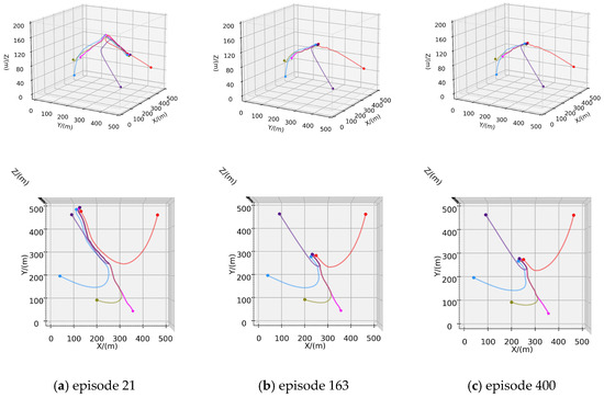
Figure 7.
Training process of Scenario B: (a) Trajectories of episode 21; (b) Trajectories of episode 163; (c) Trajectories of episode 400.
Figure 7a illustrates the trajectory of the hunter’s first successful hunting in the 500-episode experimental scenario, approaching the evader within a range of 1 m. Similar to the 1v1 pursuit–evasion scenario, the evader is hunted before it approaches the designated escape boundary, resulting in a relatively long pursuit and evasion path. However, the speed advantage of the hunters over the evader is intentionally weakened in this scenario. Under this premise, the hunters achieve their first successful hunting with fewer episodes (21 episodes) than in Scenario A. As training iterations increase, the pursuit and evasion paths gradually shorten, and the time required for successful hunting decreases, as shown in Figure 7b,c. The increase in training iterations determines that the hunters tend to employ shorter paths to achieve faster hunting. Figure 8 presents the relevant curves of this process, and Figure 8a displays the cumulative hunting and escape success rates for both the hunter and the evader as training iterations increase. Figure 8b–d, respectively, show the conclusion steps, total rewards per episode, and the average rewards per step for both the hunter and the evader. In the three curves of Scenario A, due to the weak speed advantage of hunters and the lack of multiple AUVs to restrict the escape of the evader, the reward curves of the evader in Figure 8c,d exhibit a relatively slow declining trend. However, in this scenario, a significant numerical advantage of hunters enables them to better constrain the escape of evader. Compared to the curves in Scenario A, the reward curve of the evader exhibits a more pronounced declining trend.
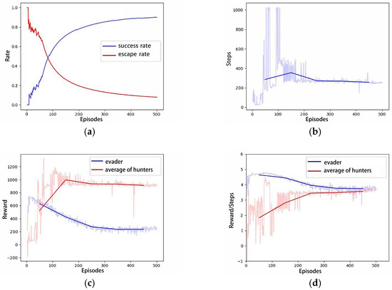
Figure 8.
The curves of Scenario B: (a) Success rate; (b) Steps; (c) Total Rewards; (d) Average Rewards per step.
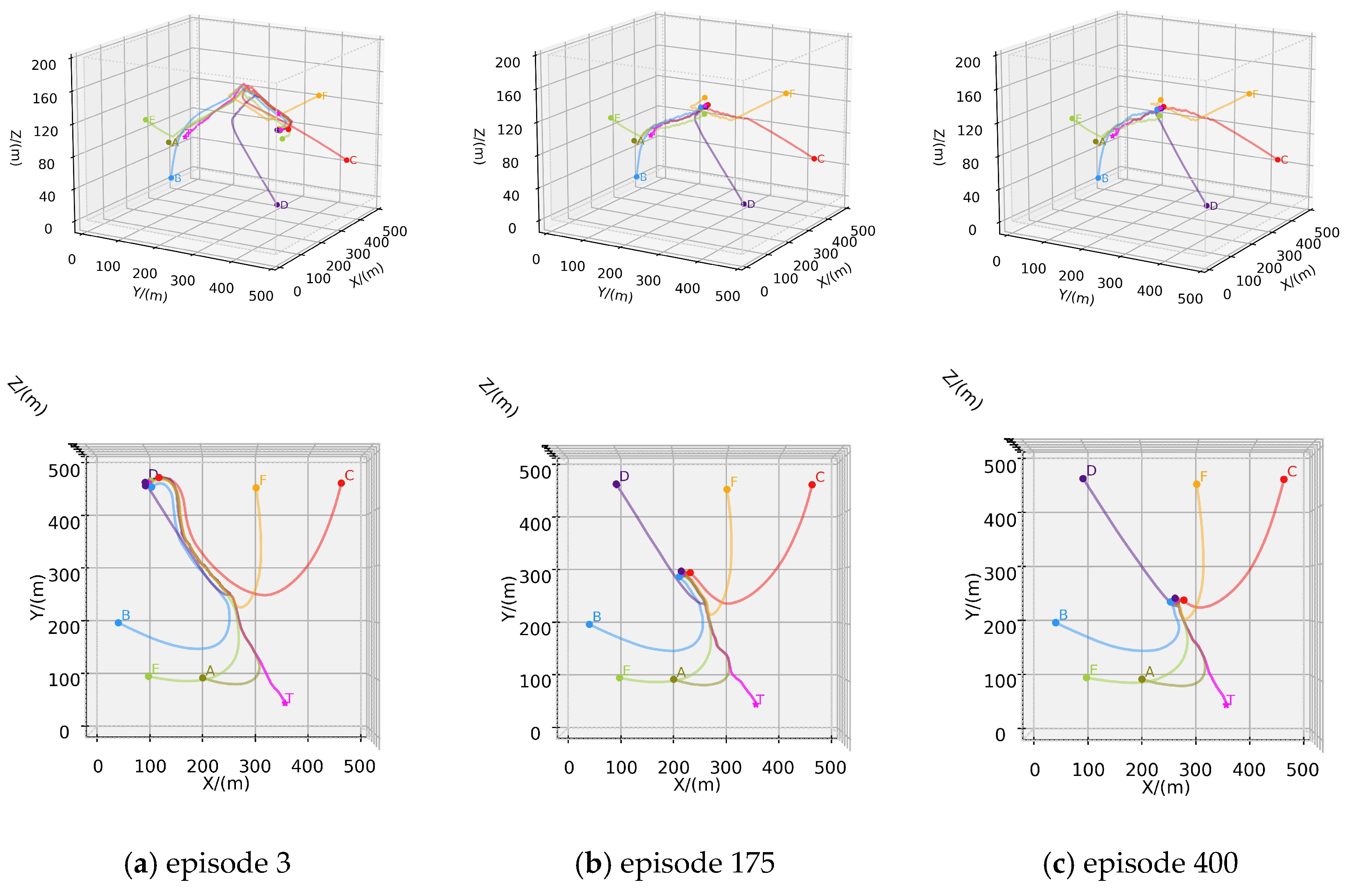
4.2.3. Scenario C: Six Hunters–One Evader Game
In this scenario, six hunters are deployed to pursue the evader, and strategically positioned in the designated environment. The initial position of the AUV is . The maximum speed of each hunter is reduced to 2.6 m/s, while the evader maintains a maximum speed of 2.5 m/s. Other configurations are identical to those in Scenario B. In the 500-episode test scenario, the trajectories of the hunters and the evader are depicted in Figure 9, where the pink line represents the trajectory of the evader, and the other lines indicate the trajectories of the hunters.
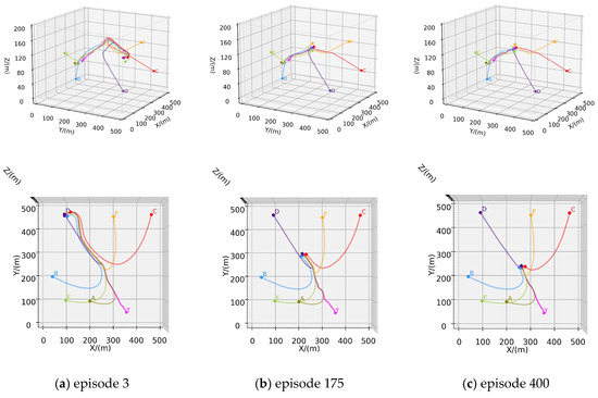
Figure 9.
Training process of Scenario C: (a) Trajectories of episode 3; (b) Trajectories of episode 175; (c) Trajectories of episode 400.
In comparison to Scenario B, scenario C aims to explore the algorithm’s capability to support a larger-scale hunting group and whether the performance satisfies expectations. Intuitively, six hunters should hunt the evader faster and easier. Figure 9a indicates that Scenario C successfully hunted for the first time in only three episodes under similar initial conditions. Similarly, as training iterations increase, the pursuit and evasion paths gradually shorten, and the time required for successful hunting decreases, as shown in Figure 9b,c. Figure 10 presents the relevant curves of this process. Compared to the curves in Scenario B, the reward curve of the evader in Scenario C exhibits faster decline, and earlier convergence. This indicates that six hunters impose stronger constraints on the evader’s escape; that is, the algorithm maintains good performance as the number of hunters in the hunting group increases.
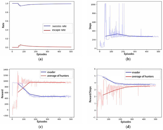
Figure 10.
The curves of Scenario C: (a) Success rate; (b) Steps; (c) Total Rewards; (d) Average Rewards per step.
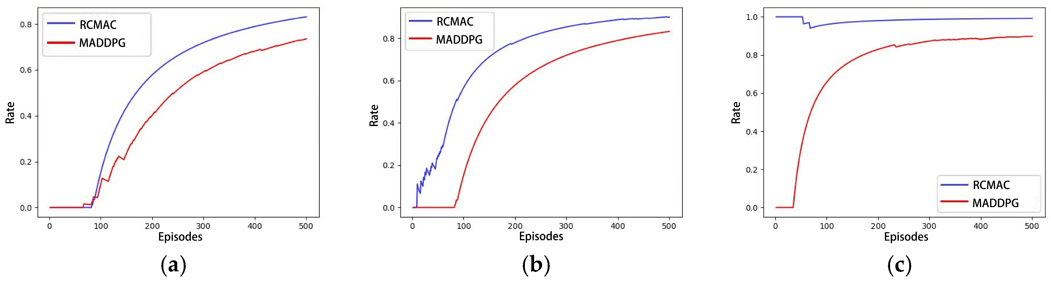
4.2.4. Performance Comparison with MADDPG
In the same simulated experimental setting as Scenario C, the training curves of MADDPG and RCMAC are represented as the average rewards obtained by six hunters. Figure 11 illustrates that the average reward obtained by hunters in the RCMAC algorithm is higher than that of the MADDPG algorithm, and the number of steps required for the successful hunting is fewer than that of MADDPG algorithm. This suggests that RCMAC tends to capture the evader faster through more efficient paths. Figure 12 presents the success rate curves of hunting using RCMAC and MADDPG in the aforementioned three scenarios, and it can be observed that MADDPG also exhibits a similar trend. The increase in the number of captors results in earlier detection and successful hunt of the evader. However, RCMAC consistently demonstrates a higher hunting success rate than MADDPG in each scenario.
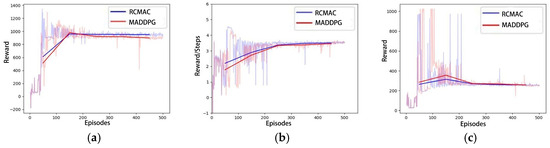
Figure 11.
The comparison between RCMAC and MADDPG: (a) Total Rewards; (b) Average Rewards per step; (c) Steps.

Figure 12.
Hunting success rate for RCMAC and MADDPG: (a) Scenario A; (b) Scenario B; (c) Scenario C.
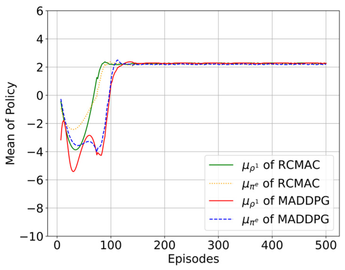
As shown in Figure 13, the learning curves of policy mean of RCMAC and MADDPG are compared over 500 episodes. It can be observed that RCMAC achieves faster convergence in competitor policy modeling () compared to MADDPG. Specifically, the competitor model in RCMAC reaches its optimal value earlier than its corresponding actual policy (), indicating that RCMAC can accurately anticipate competitor strategies in advance during training. In contrast, although MADDPG also converges to the optimal policy ultimately, its competitor model exhibits slower convergence and only catches up with the actual policy at later training stages. This implies that RCMAC can establish a more reliable competitor model earlier, providing stronger strategic guidance during policy optimization. Overall, these results validate the effectiveness of the proposed algorithm in enhancing learning efficiency compared to baseline methods.
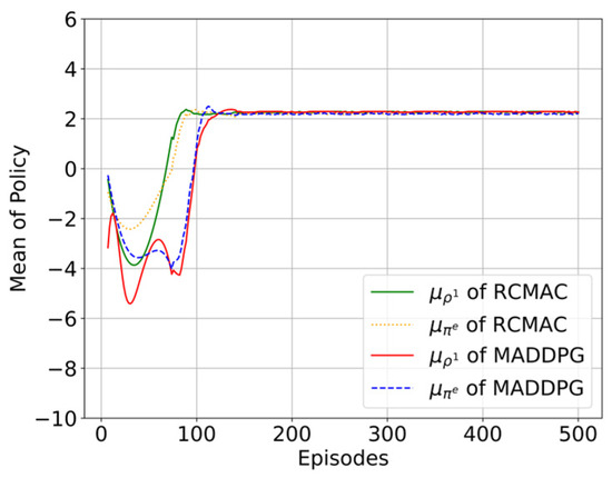
Figure 13.
The comparison of policy modeling curves between RCMAC and MADDPG.
5. Conclusions
This paper investigates a competitive game process among agents in MARL. An optimality operator is introduced to establish a competitor model during the training process and to reconstruct the objective function. Based on this approach, the RCMAC algorithm is proposed and applied to a scenario involving multiple AUVs hunting evading targets in a 3D underwater environment. The evader is treated as an intelligent agent with learning capabilities; its escape ability is optimized through training, thereby enhancing the randomness of its actions and simulating more complex hunting scenarios. This training strategy enriches the complexity and diversity of the simulated environment, enabling the hunting AUVs’ policies to achieve greater adaptability. In the simulation experiments, RCMAC demonstrated superior convergence and performance across multiple competitive game scenarios. Specifically, as shown in Figure 11, the average cumulative rewards obtained by RCMAC are consistently higher than those achieved by MADDPG across different test scenarios. Figure 12 further shows that RCMAC achieved a higher hunting success rate compared to the baseline MADDPG algorithm. Moreover, the learning curves presented in Figure 13 illustrate that RCMAC converges faster in both policy optimization and competitor modeling.
Overall, these results validate the effectiveness of the proposed RCMAC algorithm in improving learning efficiency and task performance in multi-agent competitive environments. For future work, we plan to address the challenges encountered in larger-scale AUV hunting scenarios, where the computational burden and training time significantly increase due to the expansion of the action and state spaces. Reducing computational complexity and improving training efficiency to enhance the scalability of MARL algorithms in larger team settings will be an important focus of our future research.
Author Contributions
Conceptualization, Y.S. and Z.W.; methodology, Y.S. and Z.W.; software, Y.S. and Z.W.; validation, Y.S., Z.W. and H.L.; formal analysis, Y.S., Z.W. and H.L.; investigation, G.B. and Z.W.; resources, G.B. and Z.W.; data curation, Z.W. and Y.S.; writing—original draft preparation, Y.S.; writing—review and editing, Y.S. and Z.W.; visualization, Y.S.; supervision, G.B. and Z.W.; project administration, G.B. and Z.W.; funding acquisition, Z.W. All authors have read and agreed to the published version of the manuscript.
Funding
This research was funded by the National Key Research and Development Program of China under Grant No. 2023YFB4707003 and the National Natural Science Foundation of China under Grant 52131101, Grant 52025111.
Data Availability Statement
The original contributions presented in this study are included in the article. Further inquiries can be directed to the corresponding author.
Conflicts of Interest
The authors declare no conflicts of interest.
Abbreviations
| AUV | Autonomous Underwater Vehicle |
| RCM | Regularized Competitor Model |
| RCMAC | Regularized Competitor Model with Maximum Entropy Objective Actor-Critic |
| DRL | Deep Reinforcement Learning |
| MARL | Multi-Agent Reinforcement Learning |
| DDPG | Deep Deterministic Policy Gradient |
| MADDPG | Multi-Agent Deep Deterministic Policy Gradient |
| CTDE | centralized training and decentralized execution |
| SAC | Soft Actor-Critic |
References
- Ma, T.; Lyu, J.; Yang, J.; Xi, R.; Li, Y.; An, J.; Li, C. CLSQL: Improved Q-Learning Algorithm Based on Continuous Local Search Policy for Mobile Robot Path Planning. Sensors 2022, 22, 5910. [Google Scholar] [CrossRef] [PubMed]
- Cao, X.; Sun, H.; Guo, L. Potential Field Hierarchical Reinforcement Learning Approach for Target Search by Multi-AUV in 3-D Underwater Environments. Int. J. Control 2020, 93, 1677–1683. [Google Scholar] [CrossRef]
- Wang, G.; Wei, F.; Jiang, Y.; Zhao, M.; Wang, K.; Qi, H. A Multi-AUV Maritime Target Search Method for Moving and Invisible Objects Based on Multi-Agent Deep Reinforcement Learning. Sensors 2022, 22, 8562. [Google Scholar] [CrossRef] [PubMed]
- Mao, Y.; Gao, F.; Zhang, Q.; Yang, Z. An AUV Target-Tracking Method Combining Imitation Learning and Deep Reinforcement Learning. J. Mar. Sci. Eng. 2022, 10, 383. [Google Scholar] [CrossRef]
- Jiang, Y.; Zhao, M.; Wang, C.; Wei, F.; Qi, H. A Method for Underwater Human–Robot Interaction Based on Gestures Tracking with Fuzzy Control. Int. J. Fuzzy Syst. 2021, 23, 2170–2181. [Google Scholar] [CrossRef]
- Wu, C.; Dai, Y.; Shan, L.; Zhu, Z. Date-Driven Tracking Control via Fuzzy-State Observer for AUV under Uncertain Disturbance and Time-Delay. J. Mar. Sci. Eng. 2023, 11, 207. [Google Scholar] [CrossRef]
- Wu, J.; Song, C.; Ma, J.; Wu, J.; Han, G. Reinforcement Learning and Particle Swarm Optimization Supporting Real-Time Rescue Assignments for Multiple Autonomous Underwater Vehicles. IEEE Trans. Intell. Transp. Syst. 2022, 23, 6807–6820. [Google Scholar] [CrossRef]
- Cao, X.; Zuo, F. A Fuzzy-Based Potential Field Hierarchical Reinforcement Learning Approach for Target Hunting by Multi-AUV in 3-D Underwater Environments. Int. J. Control 2021, 94, 1334–1343. [Google Scholar] [CrossRef]
- Chen, M.; Zhu, D. A Novel Cooperative Hunting Algorithm for Inhomogeneous Multiple Autonomous Underwater Vehicles. IEEE Access 2018, 6, 7818–7828. [Google Scholar] [CrossRef]
- Chen, L.; Guo, T.; Liu, Y.; Yang, J. Survey of Multi-Agent Strategy Based on Reinforcement Learning. In Proceedings of the 2020 Chinese Control and Decision Conference (CCDC), Hefei, China, 22–24 August 2020; pp. 604–609. [Google Scholar]
- Orr, J.; Dutta, A. Multi-Agent Deep Reinforcement Learning for Multi-Robot Applications: A Survey. Sensors 2023, 23, 3625. [Google Scholar] [CrossRef] [PubMed]
- Cao, X.; Xu, X. Hunting Algorithm for Multi-AUV Based on Dynamic Prediction of Target Trajectory in 3D Underwater Environment. IEEE Access 2020, 8, 138529–138538. [Google Scholar] [CrossRef]
- Lu, R.; Li, Y.-C.; Li, Y.; Jiang, J.; Ding, Y. Multi-Agent Deep Reinforcement Learning Based Demand Response for Discrete Manufacturing Systems Energy Management. Appl. Energy 2020, 276, 115473. [Google Scholar] [CrossRef]
- Lowe, R.; WU, Y.; Tamar, A.; Harb, J.; Pieter Abbeel, O.; Mordatch, I. Multi-Agent Actor-Critic for Mixed Cooperative-Competitive Environments. In Proceedings of the Advances in Neural Information Processing Systems, Long Beach, CA, USA, 4–9 December 2017; Guyon, I., Luxburg, U.V., Bengio, S., Wallach, H., Fergus, R., Vishwanathan, S., Garnett, R., Eds.; Curran Associates, Inc.: Red Hook, NY, USA, 2017; Volume 30. [Google Scholar]
- Tian, Z.; Wen, Y.; Gong, Z.; Punakkath, F.; Zou, S.; Wang, J. A Regularized Opponent Model with Maximum Entropy Objective. In Proceedings of the 28th International Joint Conference on Artificial Intelligence, Macao, China, 10–16 August 2019. [Google Scholar]
- Castillo-Zamora, J.J.; Camarillo-Gómez, K.A.; Pérez-Soto, G.I.; Rodríguez-Reséndiz, J.; Morales-Hernández, L.A. Mini-AUV Hydrodynamic Parameters Identification via CFD Simulations and Their Application on Control Performance Evaluation. Sensors 2021, 21, 820. [Google Scholar] [CrossRef] [PubMed]
- Rashid, T.; Samvelyan, M.; De Witt, C.S.; Farquhar, G.; Foerster, J.; Whiteson, S. Monotonic Value Function Factorisation for Deep Multi-Agent Reinforcement Learning. J. Mach. Learn. Res. 2020, 21, 1–51. [Google Scholar]
- Foerster, J.; Song, F.; Hughes, E.; Burch, N.; Dunning, I.; Whiteson, S.; Botvinick, M.; Bowling, M. Bayesian Action Decoder for Deep Multi-Agent Reinforcement Learning. In Proceedings of the 36th International Conference on Machine Learning, PMLR, Long Beach, CA, USA, 24 May 2019; pp. 1942–1951. [Google Scholar]
- Nayyar, A.; Mahajan, A.; Teneketzis, D. Decentralized Stochastic Control with Partial History Sharing: A Common Information Approach. IEEE Trans. Autom. Control 2013, 58, 1644–1658. [Google Scholar] [CrossRef]
- Wen, Y.; Yang, Y.; Luo, R.; Wang, J.; Pan, W. Probabilistic Recursive Reasoning for Multi-Agent Reinforcement Learning. In Proceedings of the 7th International Conference on Learning Representations, ICLR 2019, New Orleans, LA, USA, 6–9 May 2019. [Google Scholar]
- Davies, I.; Tian, Z.; Wang, J. Learning to Model Opponent Learning. In Proceedings of the 34th AAAI Conference on Artificial Intelligence (AAAI-20), New York, NY, USA, 7–12 February 2020. [Google Scholar]
- Zhu, Q.; Başar, T. Decision and Game Theory for Security; Springer: Fort Worth, TX, USA, 2013; pp. 246–263. [Google Scholar]
- Haarnoja, T.; Tang, H.; Abbeel, P.; Levine, S. Reinforcement Learning with Deep Energy-Based Policies. In Proceedings of the International Conference on Machine Learning, PMLR, Long Beach, CA, USA, 6–11 August 2017; pp. 1352–1361. [Google Scholar]
- Haarnoja, T.; Zhou, A.; Abbeel, P.; Levine, S. Soft Actor-Critic: Off-Policy Maximum Entropy Deep Reinforcement Learning with a Stochastic Actor. In Proceedings of the International Conference on Machine Learning, PMLR, Long Beach, CA, USA, 10–15 July 2018; pp. 1861–1870. [Google Scholar]
- Haarnoja, T.; Zhou, A.; Hartikainen, K.; Tucker, G.; Ha, S.; Tan, J.; Kumar, V.; Zhu, H.; Gupta, A.; Abbeel, P.; et al. Soft Actor-Critic Algorithms and Applications. arXiv 2019, arXiv:1812.05905. [Google Scholar]
- Wei, E.; Wicke, D.; Freelan, D.; Luke, S. Multiagent Soft Q-Learning. arXiv 2018, arXiv:1804.09817. [Google Scholar]
- Danisa, S. Learning to Coordinate Efficiently through Multiagent Soft Q-Learning in the Presence of Game-Theoretic Pathologies. Master’s Thesis, University of Cape Town, Cape Town, Western Cape, South Africa, September 2022. [Google Scholar]
- Fjellstad, O.-E.; Fossen, T.I. Position and Attitude Tracking of AUV’s: A Quaternion Feedback Approach. IEEE J. Ocean. Eng. 2002, 19, 512–518. [Google Scholar] [CrossRef]
- Wang, Z.; Sui, Y.; Qin, H.; Lu, H. State Super Sampling Soft Actor–Critic Algorithm for Multi-AUV Hunting in 3D Underwater Environment. J. Mar. Sci. Eng. 2023, 11, 1257. [Google Scholar] [CrossRef]


Disclaimer/Publisher’s Note: The statements, opinions and data contained in all publications are solely those of the individual author(s) and contributor(s) and not of MDPI and/or the editor(s). MDPI and/or the editor(s) disclaim responsibility for any injury to people or property resulting from any ideas, methods, instructions or products referred to in the content. |
© 2025 by the authors. Licensee MDPI, Basel, Switzerland. This article is an open access article distributed under the terms and conditions of the Creative Commons Attribution (CC BY) license (https://creativecommons.org/licenses/by/4.0/).