Article

High-Resolution Underwater Imaging via Richardson–Lucy Deconvolution Beamforming with Acoustic Frequency Comb Excitation

1
School of Marine Science and Technology, Tianjin University, Tianjin 300072, China
2
Key Laboratory of Marine Environmental Survey Technology and Application, Ministry of Nature Resources, Guangzhou 510300, China
*
Author to whom correspondence should be addressed.
J. Mar. Sci. Eng. 2025, 13(12), 2290; https://doi.org/10.3390/jmse13122290
Submission received: 2 November 2025 / Revised: 27 November 2025 / Accepted: 27 November 2025 / Published: 2 December 2025

Abstract

Underwater acoustic imaging is essential in marine science and engineering, enabling high-resolution detection and characterization of underwater structures and targets. However, conventional deconvolution beamforming methods using broadband signals often suffer from model mismatch, inter-frequency interference, and limited noise robustness. To overcome these challenges, this study rigorously analyzes the point spread function of the imaging system and introduces Acoustic Frequency Comb (AFC) excitations to enhance resolution. By exploiting the autocorrelation characteristics of AFC signals and optimizing key parameters, imaging artifacts are effectively suppressed and the main-lobe width is narrowed, resulting in a 50% improvement in range resolution. Comparative analyses identify the Richardson–Lucy algorithm as the most effective in enhancing azimuthal resolution and maintaining robustness under array perturbations and low signal-to-noise ratios. Parametric studies further demonstrate that AFC excitation outperforms conventional linear frequency modulated pulses, achieving a 30% main-lobe width reduction, 10 dB sidelobe suppression, and a 14 dB noise decrease. Finally, tank experiments confirm the simulation results, showing that accurate PSF modeling enabled by AFC ensures high angular resolution. The discrete spectral structure facilitates more effective separation of signal and noise during iterative deconvolution, while excellent autocorrelation characteristics guarantee high range resolution, yielding superior overall imaging performance.

1. Introduction

Underwater acoustic imaging technology plays a vital role in marine science and engineering, with important applications in shipwreck salvage, marine surveying, and target detection [1,2,3]. As ocean exploration advances, the growing demand for underwater high-resolution imaging has driven significant innovations in sonar technology, leading to the development of diverse methods such as side-scan, acoustic lens, synthetic aperture, and multibeam sonar [4,5,6,7]. Among these, Conventional Beamforming (CBF) methods remain widely used due to their computational simplicity, fast imaging speed, and strong robustness [8]. Multibeam imaging technology significantly enhances underwater image resolution by optimizing acoustic beam transmission and reception [9], facilitating detailed and precise imaging even in complex marine environments. With continuous advancements in signal processing techniques, multibeam imaging methods are evolving to meet increasingly demanding resolution requirements and operational conditions [10]. However, the resolution of CBF is fundamentally constrained by the physical aperture of the array, limiting its ability to achieve high-precision imaging. This inherent constraint has emerged as a critical bottleneck impeding the development and practical deployment of high-resolution underwater imaging technologies.
Several high-resolution algorithms have been developed to address this limitation. Classical methods such as the Minimum Variance Distortionless Response (MVDR) [11] enhance angular resolution by minimizing output power through spatial filtering. Subspace-based algorithms, including Multiple Signal Classification (MUSIC) [12] and Estimation of Signal Parameters via Rotational Invariance Techniques (ESPRIT) [13], exploit the orthogonality between signal and noise subspaces via eigenvalue decomposition of the covariance matrix, enabling high-resolution angular imaging. Although these methods theoretically offer high angular resolution capabilities, their performance is highly sensitive to the number of sources, Signal-to-Noise Ratio (SNR), and snapshot count. Moreover, challenges related to stability and robustness in complex underwater environments significantly limit their practical applicability. To mitigate these challenges, deconvolution-based beamforming methods have attracted increasing attention. Techniques such as Deconvolution Approach for the Mapping of Acoustic Sources (DAMAS) [14], Non-Negative Least Squares (NNLS) [15], and Richardson–Lucy (RL) [16] perform deconvolution to recover the source distribution from the beam pattern using the known Point Spread Function (PSF), thereby achieving enhanced resolution without relying on subspace decomposition or strong prior information, while exhibiting superior robustness and practical applicability.
However, conventional deconvolution algorithms encounter substantial computational challenges in broadband acoustic imaging. The requirement to perform convolution and iterative solutions at each frequency point results in high computational complexity, which becomes particularly pronounced in wideband signal processing. To address this issue, researchers have proposed various acceleration strategies based on classical deconvolution methods. Dougherty transformed the spatial convolution between the source distribution and the PSF into a multiplication in the wavenumber domain, leading to the Fast Fourier Transform (FFT)-based DAMAS2 algorithm. This was further extended to DAMAS3 [17] by incorporating low-rank compression techniques, significantly improving computational efficiency. Building on this work, Ehrenfried from the German Aerospace Center proposed the FFT-NNLS algorithm [18], which embeds NNLS into the Fourier-domain deconvolution framework, achieving notable improvements in both accuracy and convergence speed. Subsequently developed methods such as sparsity-constrained-DAMAS [19], fast wavelet DAMAS [20], and FFT-FISTA [21], have also made promising advances in compressive sensing and transform-domain modeling.
Despite improvements in computational efficiency, existing methods remain limited in modeling accuracy. Fourier transform-based deconvolution acceleration strategies typically construct PSFs at a finite set of discrete frequencies to approximate the full-band system response. However, under broadband conditions, CBF outputs are obtained by integration over the entire frequency band, which results in inherent inconsistencies between the discrete-frequency PSFs and the full-band CBF. This modeling mismatch fundamentally degrades resolution, and inter-frequency coupling further exacerbates the problem. Additionally, the continuous spectrum of the signal is highly coupled with environmental noise, making it difficult to effectively separate the signal from noise through iterative deconvolution under low-SNR conditions. To address these issues, optimizing the design of the transmitted signal presents an effective solution for enhancing imaging performance. The Acoustic Frequency Comb (AFC) signal [22], characterized by its spectral discreteness and low inter-frequency coherence, provides an effective means to resolve the modeling mismatch. The AFC consists of uniformly spaced narrowband frequency components, ensuring alignment between the beamforming output and the PSF. Furthermore, its spectrum, distinct from environmental noise, allows for more efficient signal isolation during iterative deconvolution, significantly enhancing noise performance in the imaging process.
Leveraging the inherent advantages of AFC signals, this study systematically investigated their application in deconvolution-based beamforming for underwater acoustic imaging. We first analyzed the PSF characteristics and exploited the distinctive autocorrelation structure of AFC signals to guide parameter optimization, which enabled effective suppression of range-domain artifacts and achieved an approximate 50% improvement in range resolution. To further enhance angular resolution, multiple deconvolution algorithms were evaluated, with the RL method ultimately selected as the core framework due to its superior performance and algorithmic stability. Controlled simulations were then conducted to assess the effectiveness and robustness of the proposed AFC-RL approach under various conditions, including array element misalignments and low SNR. Parametric studies were also conducted on SNR, sub-band count, and iteration number. Compared with conventional Linear Frequency Modulated (LFM) signals of identical bandwidth, the AFC-RL method achieved roughly 30% improvement in main-lobe compression, a 10 dB reduction in sidelobe level, an approximately 14 dB improvement in noise suppression, and enhanced weak-target detectability. Finally, controlled tank experiments further confirm the simulation results, validating the practical feasibility of the proposed AFC-RL imaging approach and providing a thorough analysis and discussion of its imaging performance.

2. Materials and Methods

2.1. Broadband Signal Deconvolution Beamforming

CBF achieves directional control of the main lobe by applying phase shifts or time delays across array elements, thereby ensuring that the array output exhibits well-defined spatial directivity. This operation can be interpreted as a form of spatial filtering, designed to enhance signals from desired directions while effectively suppressing interference and noise from other directions. From an imaging perspective, the beam direction encodes information about the target’s azimuth, while the echo return time provides range information. Consequently, beamforming enables the reconstruction of a two-dimensional image representing both distance and direction within the coverage area. Beamforming-based imaging is fundamental to underwater detection and imaging applications. By appropriately weighting and coherently combining the received signals, the method can enhance target signals and suppress background noise, thereby significantly improving the SNR and facilitating the detection of weak targets. Further applying pulse compression to each beam enables the acquisition of high-resolution results in the range direction. The detailed procedure is illustrated in Figure 1.
The signal received by the m-th element of a uniform linear array (ULA), for m = 1, …, M, can be expressed as:
s m t = n = 1 N T a n t τ m , n + n m t ,
where N T is the number of target signal sources, a n ( t ) represents the echo signal from the n-th target, τ m , n denotes the time delay of the n-th target signal arriving at element m , and n m represents the noise component in the signal received by element m .
Therefore, the expression of time-domain beamforming is given as:
y t , θ = m = 1 M ω m s m t + τ m θ ,
where τ m θ = m d s i n θ / c . A commonly used distortionless weighting scheme is to set ω m = 1 , or it can be normalized to ω m = 1 / M .
A ULA requires a certain mapping transformation to satisfy the shift-invariance condition. Its inherent directivity function can be expressed as:
B p θ = s i n ( N π d λ c o s θ ) N s i n ( π d λ c o s θ ) 2 .
Furthermore, the directivity function in the angular ϑ direction is given by:
B p θ ϑ = s i n ( N π d λ ( c o s θ c o s ϑ ) ) N s i n ( π d λ ( c o s θ c o s ϑ ) ) 2 .
The signal is squared here to ensure consistency with the CBF power spectrum. From Equation (4), we can easily obtain:
B p θ ϑ B p θ ϑ .
Thus, a convolution process cannot directly replace the superposition process. However, after a simple transformation, the natural directivity function of a uniform linear array exhibits shift-invariant property of c o s θ , that is:
B p c o s θ c o s ϑ = B p c o s θ c o s ϑ .
According to Equation (6), the beamforming output P of a ULA can be equivalently represented as a convolution process:
P c o s θ = B p c o s θ c o s ϑ S c o s ϑ d c o s ϑ = B p c o s θ S c o s θ .
Based on the above analysis, under the assumption of array shift-invariance, the spatial distribution of signal sources can be accurately reconstructed via deconvolution.
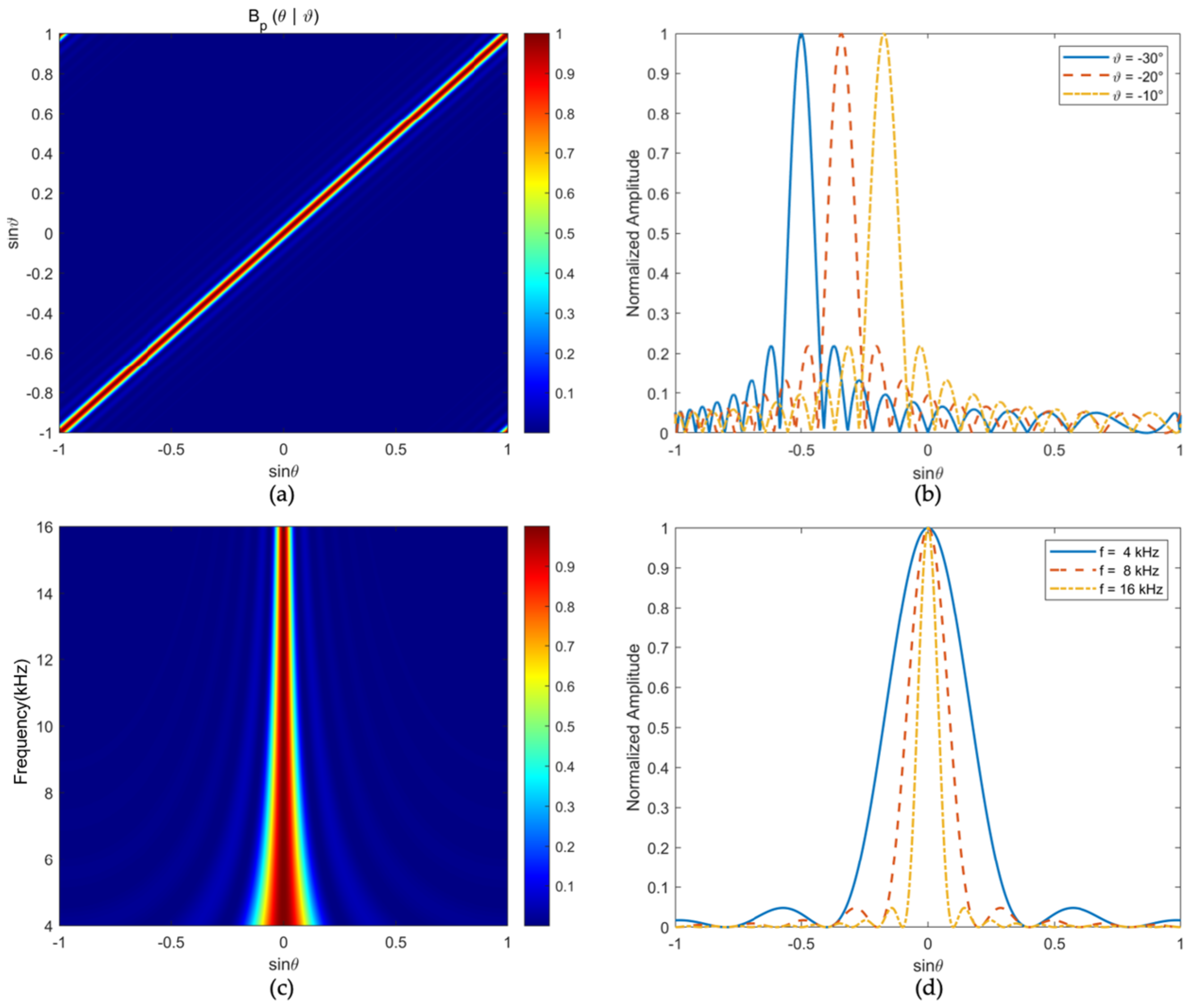
The directional function pointing to different angles is independent of the angle and has shift invariance. It can be regarded as a shift of the natural directional function, as shown in Figure 2a,b.
For broadband signals, the wavelength λ is not a single value. Therefore, the spacing between array elements does not always equal half the wavelength corresponding to the signal frequency. This discrepancy can lead to larger errors in detecting and estimating the signals, thereby degrading the resolution performance. As a result, broadband signals cannot be directly processed using the narrowband signal model. Furthermore, PSF can also be expressed as follows:
P S F f = s i n [ π N d f c c o s θ c o s ϑ ] N s i n [ π d f c c o s θ c o s ϑ ] 2 .
From Equation (8), the PSF is a deterministic function that depends solely on the array structure parameters (number of elements, element spacing, and signal wavelength), which can be pre-calculated during the array design phase. Under a fixed array configuration, the PSFs corresponding to different frequencies are also distinct, as illustrated in Figure 2c,d. The source distribution S is typically modeled as a series of directional δ functions, reflecting the spatial distribution characteristics of the sound source. The CBF output P can be directly obtained from the receiving array. By performing deconvolution on P, the S can be estimated, enabling high-resolution localization and recognition of spatial targets.
Broadband deconvolution beamforming requires performing deconvolution at each frequency by processing the CBF output with the corresponding PSF, thereby obtaining the source distribution function S(f) at that frequency. The results across all K frequencies are then coherently summed to yield the final spatial source distribution, as shown in Equation (9).
S θ = k = 0 K 1 S f k , θ .

2.2. Comparison of Deconvolution Methods

Traditional deconvolution beamforming methods iteratively invert CBF images using the PSF model, thereby effectively suppressing sidelobes, sharpening the main lobe, and enhancing the SNR. These approaches enable high-resolution imaging without relying on strong prior assumptions. By achieving a favorable balance among spatial resolution, robustness, and computational efficiency, such methods have emerged as a critical technical pathway for advancing underwater imaging quality. In the following, several widely adopted algorithms, including DAMAS, NNLS, and the RL method, are comparatively analyzed to highlight their advantages, and limitations.
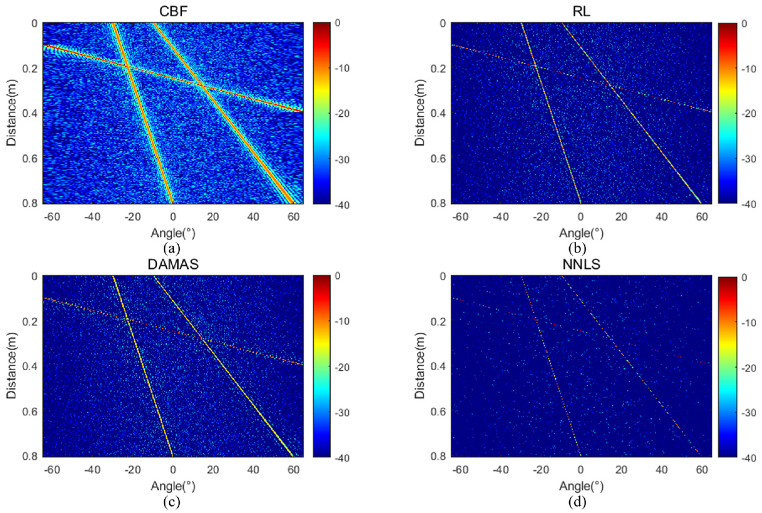
To evaluate the performance of different beamforming methods in enhancing imaging resolution, this study compares the imaging results of three typical deconvolution algorithms: DAMAS, NNLS, and RL. Figure 3 simulates three cross-line targets at 0.8 m, with angles ranging from −60° to −30°, −30° to 0°, and 0° to 60°, respectively, to clearly illustrate the angular resolution of each deconvolution beamforming method.
The results show that, compared to the CBF method (Figure 3a), all three deconvolution algorithms significantly enhance azimuth resolution, effectively suppress side lobe spread, and achieve clearer target separation and enhanced imaging. Specifically, the DAMAS (Figure 3c) method excels in suppressing far-side lobes, while NNLS (Figure 3b) has a certain advantage in reconstructing sparse target distributions. However, both methods have relatively high computational complexity and are highly dependent on the sparsity and stability of the system response matrix. In contrast, the RL (Figure 3d) deconvolution method maintains high resolution while demonstrating greater robustness and computational efficiency, making it suitable for iterative reconstruction in complex acoustic environments. Its iterative update mechanism, which combines multiplication and division operations, not only facilitates parallel acceleration but also has a certain tolerance for non-ideal modeling errors in underwater scenarios.
Considering the resolution ability, algorithm robustness, and engineering feasibility this study selects RL algorithm as the main deconvolution beamforming algorithm in underwater acoustic imaging to provide support for the subsequent high-resolution imaging comparison.

2.3. Design of the AFC Constraint Parameters

The AFC signal is composed of multiple equally spaced discrete frequency components, exhibiting sparse and structured characteristics in the frequency domain. In the time domain, it presents periodic high-amplitude narrow pulses, combining the high temporal resolution of broadband signals with the frequency consistency of multi-frequency signals. Thanks to its excellent autocorrelation performance, frequency separation, and low inter-frequency coherence, the AFC signal has become a crucial type of signal in underwater acoustic communication [23], underwater positioning [24], and Doppler estimation [25]. It also provides theoretical support for the design of high-resolution deconvolution imaging algorithms.
In the deconvolution beamforming framework described in this paper, the AFC signal is modeled as a linear superposition of K equally spaced sinusoidal subcarriers with a starting frequency of f0 and a frequency interval of f , whose time domain expression is:
s t = k = 0 K 1 A k cos 2 π f 0 + k f t + k , t [ T 2 , T 2 ] .

2.3.1. The Autocorrelation of the AFC

The autocorrelation function is defined as:
R x τ = lim T 1 T T / 2 T / 2 x ( t ) x ( t + τ ) d t .
For the convenience of calculation, the acoustic frequency comb signal is taken as a complex domain signal, and x t is expanded and substituted:
x t = n = 0 N 1 e j 2 π ( f 0 + n f ) t ,
x t + τ = m = 0 N 1 e j 2 π ( f 0 + m f ) t + τ .
The product is:
x t x t + τ = n = 0 N 1 m = 0 N 1 e j 2 π ( f 0 + n f ) t e j 2 π ( f 0 + m f ) t + τ .
Simplification yields:
x t x t + τ = n = 0 N 1 m = 0 N 1 e j 2 π [ n m f t f 0 + m f τ ] .
The time integration is:
R x τ = n = 0 N 1 m = 0 N 1 e j 2 π f 0 + m f τ lim T 1 T T 2 T 2 e j 2 π n m f t d t .
Additionally,
lim T 1 T T / 2 T / 2 e j 2 π n m f t d t = 1 , n = m 0 , n m .
Therefore, only the case n = m remains, and Formula (18) can then be obtained.
R x τ = n = 0 N 1 e j 2 π ( f 0 + n f ) τ .
Further simplification yields:
R x τ = e j 2 π f 0 τ n = 0 N 1 e j 2 π n f τ .
The second half is the sum of an arithmetic progression:
n = 0 N 1 e j 2 π n f τ = 1 e j 2 π N f τ 1 e j 2 π f τ = e j π ( N 1 ) f τ sin N π f τ sin π f τ .
Therefore, Equation (20) can be expressed as
n = 0 N 1 e j 2 π n f τ = e j 2 π f c τ sin N π f τ sin π f τ ,
where
f c = f 0 + ( N 1 ) f 2 .
Therefore, the modulus of autocorrelation is:
R x τ = s i n ( N π f τ ) s i n ( π f τ ) .
Since the actual signal is a truncated signal within a finite time window, the calculation of its autocorrelation function is limited by the integral’s upper and lower limits. Specifically, the autocorrelation function has non-zero values within the delay range of |τ| ≤ T and tends to zero at |τ| > T. This is because as the delay |τ| increases, the effective overlap between the original signal and its delayed version decreases, leading to a weakening of the autocorrelation value. Specifically, as |τ| increases from 0 to T, the effective overlap gradually diminishes, and the amplitude envelope of the autocorrelation function forms a symmetrical triangular shape. Therefore, the magnitude of the autocorrelation function of the sound comb can be expressed as:
R x τ T τ 2 sin N π f τ sin π f τ .
Since the maximum value of (T|τ|)/2 is T and the maximum value of sin(Nπ∆fτ)/sin(π∆) is N, the final expression after normalization is:
R x τ T τ T N sin N π f τ sin π f τ .

2.3.2. Anti-Artifact Design

In the acoustic beamforming system based on frequency comb excitation, the excitation signal typically consists of a set of equally spaced sine components, with a frequency interval of. After the signal is processed through a finite time window (with a duration of T) and windowing, its autocorrelation function exhibits a periodic main peak structure. The spacing between these main peaks is inversely proportional to the frequency interval, as follows:
τ 0 = 1 f .
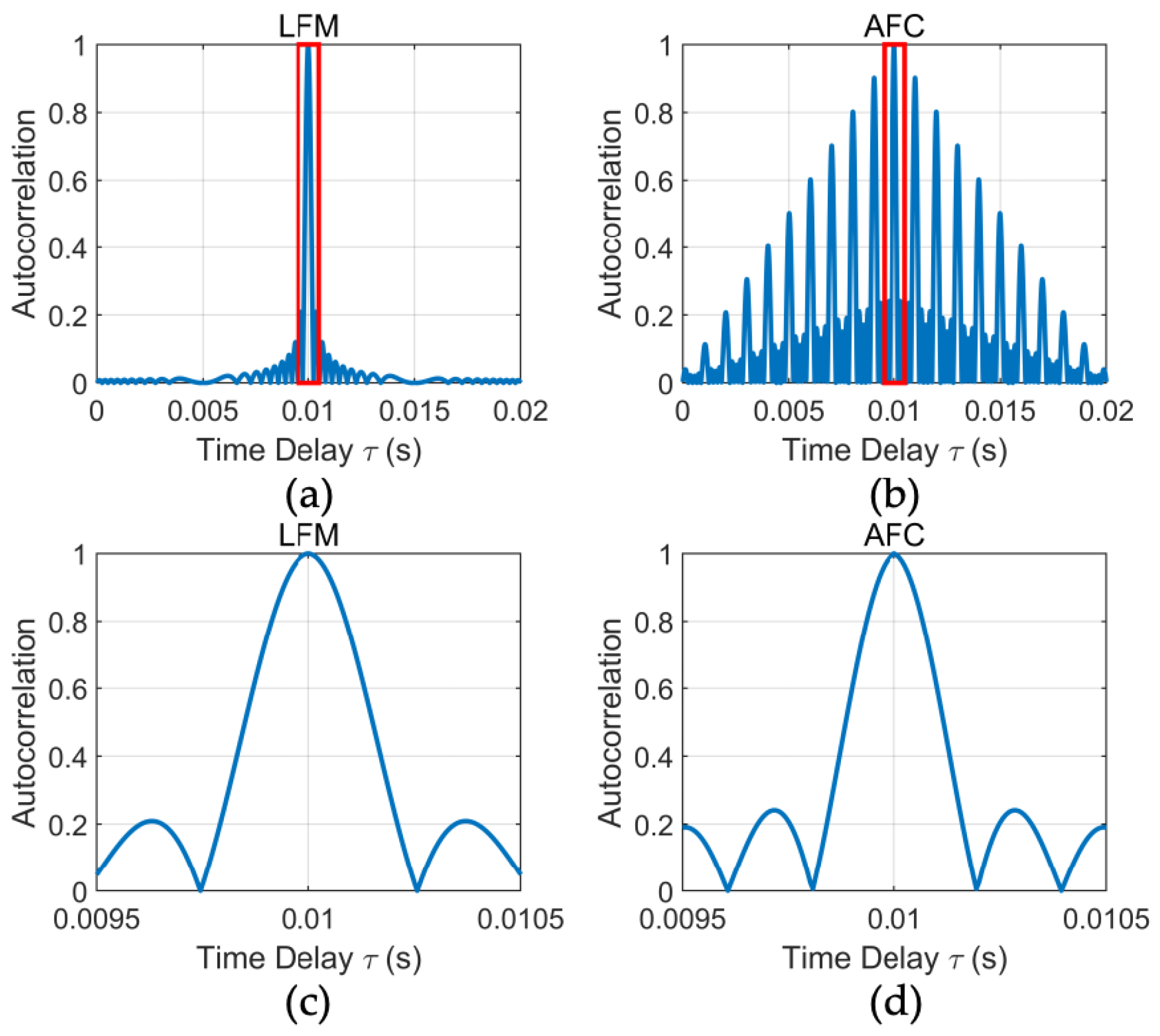
During the imaging process, if multiple target echo delays fall within the secondary peak of the autocorrelation function, matching filters or coherent superposition operations can lead to issues such as spatial ghost lobes or side lobe enhancement, as shown in Figure 4b,d. In contrast, this problem does not occur with LFM signals, as shown in Figure 4a,c.
To effectively suppress these interference effects, it is essential to ensure that the main peak of the autocorrelation function is uniquely prominent within the imaging window, while all other related peaks remain outside this window. To achieve this, the condition T τ 0 must be satisfied.
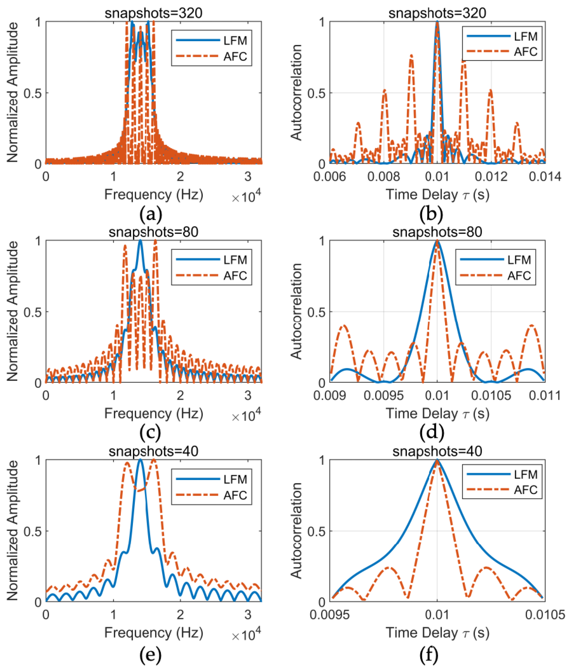
Figure 5a,b show that when signal duration T is much greater than the reciprocal of the frequency spacing τ0, the discrete spectral characteristics of the AFC signal are prominent, and the autocorrelation function exhibits periodic secondary peaks. Figure 5c,d indicate that when T equals τ0, the discrete spectral features of the AFC signal are still discernible, and the autocorrelation function displays only a single main peak, although the sidelobes remain relatively high. Figure 5e,f show that when T equals τ0/2, the autocorrelation function of the AFC signal exhibits a single main peak with reduced sidelobes, and its half-power width is narrowed by approximately 50% compared to that of the LFM signal.

2.3.3. Parameter Selection

  • Selection of frequency range
In underwater acoustic imaging, the choice of signal frequency involves a trade-off between imaging resolution and propagation loss. Higher frequencies offer shorter wavelengths, improving spatial resolution and imaging detail, but suffer from stronger absorption and scattering, reducing effective range. To balance resolution and propagation, this study selects a broadband signal of 12–16 kHz. This mid-to-low frequency range provides good underwater propagation, mitigates high-frequency attenuation, and offers sufficient bandwidth to enhance range resolution. The 4 kHz bandwidth also satisfies the frequency domain requirements of the deconvolution beamforming algorithm, ensuring imaging accuracy while maintaining signal energy efficiency. Moreover, this range is compatible with common underwater transducers, making it practical for engineering implementation.
2.
Time window and interval frequency selection
The transmitted signal’s duration must ensure temporal separation between direct and early echo signals to avoid interference, especially in shallow water or with small targets. Proper frequency intervals prevent overlapping responses that could generate false peaks in deconvolution algorithms. By aligning frequency and time characteristics, the AFC signal’s autocorrelation exhibits a single prominent main peak, effectively suppressing side lobes. This design enhances temporal resolution, reduces interference, and improves detection accuracy, ensuring reliable signal extraction even in complex environments. The frequency interval ∆f and time width T satisfy:
T = 1 / ( 2 × Δ f ) .
3.
Selection of the number and spacing of array elements
A commonly used array of 64 elements is selected for the study. During array processing, elements sample incident acoustic signals in space. Excessive spacing reduces sampling density, causing signals from different directions to have similar steering vectors, leading to spatial aliasing. This limits source localization accuracy and reliability. That is:
e j ω τ n ( θ 1 ) = e j ω τ n ( θ 2 ) ,
e j n ( 2 π d s i n θ 1 ) / λ = e j n ( 2 π d s i n θ 2 ) / λ .
To avoid aliasing, it must be satisfied with the following formulas.
2 π d s i n θ / λ θ = θ 1 , θ 2 < π ,
d s i n θ / λ < 1 / 2 .
That is, the spacing d of the array elements is lower than λ/2. Take the minimum wavelength of the frequency component and set it as the spacing of the array elements.

3. Results

3.1. Simulation Experiment

This numerical simulation experiment compares the angular resolution performance of LFM and AFC signals before and after RL deconvolution beamforming. It focuses on evaluating key metrics such as the main lobe half-power width and side lobe height, assessing the performance of both signals under various conditions, including different noise levels, multi-sub-band processing, and varying numbers of iterations. The results show that the AFC signal outperforms the LFM signal in all metrics, thus validating the effectiveness of the proposed method.

3.1.1. Position Error Performance

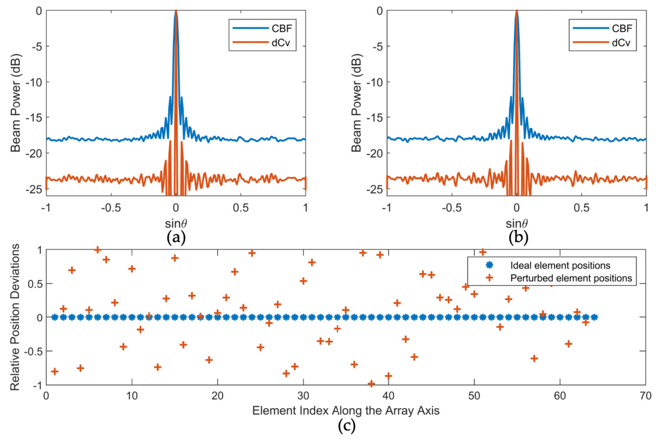
Figure 6a illustrates the results of conventional beamforming and deconvolution beamforming based on AFC signals under ideal array conditions (no element position error). Figure 6b shows the performance changes in the two methods when element position errors are introduced, with the corresponding element perturbations shown in Figure 6c. Both sets of experiments were conducted with an SNR of 0 dB.
The results show that the position error of the array elements has a minimal impact on the main lobe width and side lobe suppression capability of the beam. The deconvolution beamforming demonstrates great robustness to array errors while maintaining resolution. This suggests that the beamforming method based on AFC signals has a certain tolerance for errors in practical applications.

3.1.2. SNR Performance

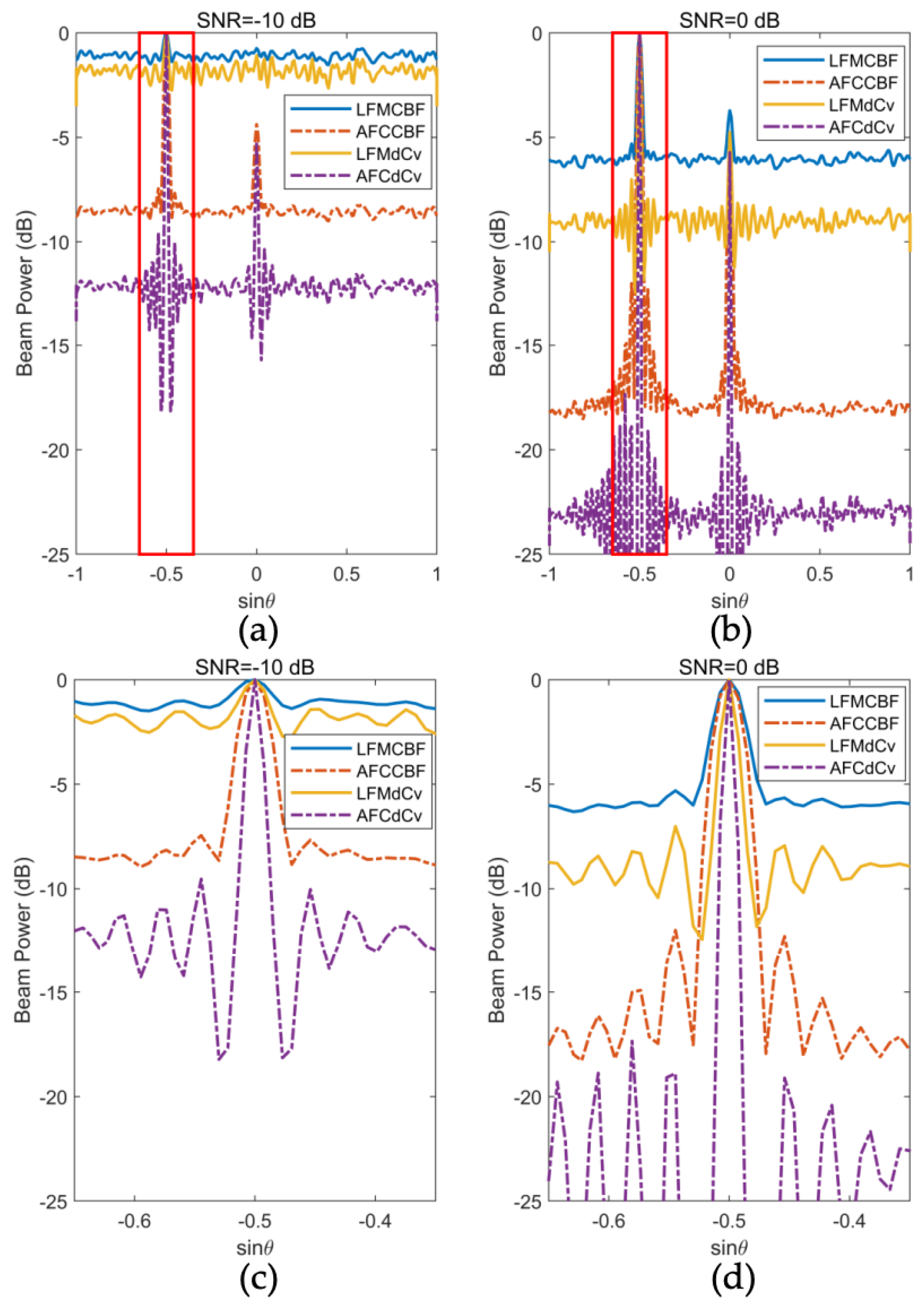
To further evaluate the noise robustness and resolution performance of different signals, Figure 7a,b illustrate the CBF and its deconvolution results of LFM and AFC signals under −10 dB and 0 dB SNR conditions, respectively. These figures are obtained in the same noise environment for both signals, with the SNR referenced to the AFC signal. Figure 7c,d provide detailed views of the red box areas, aiding in the analysis of noise performance and weak target detection capabilities. In the simulation scenario, a strong target and a weak target are set up, with an energy ratio of 4, to evaluate the resolution performance of each method. Imaging performance is assessed by measuring the beam’s half-power width (3 dB width) to quantify the main lobe width, while the maximum sidelobe amplitude indicates sidelobe strength.
As illustrated in Figure 7a,c, under an SNR of −10 dB, both the CBF and RL deconvolution results of the LFM signal fail to effectively detect weak targets. In contrast, the AFC signal can still clearly resolve weak targets under the same conditions, exhibiting a narrower main lobe, lower sidelobe levels, and a significant level of noise suppression. These results indicate that the AFC signal demonstrates superior noise robustness and weak target detection capability in low SNR environments.
Figure 7b,d present similar findings at an SNR of 0 dB. After deconvolution, the AFC signal achieves an approximately 30% reduction in main-lobe width compared to the LFM signal, along with about 10 dB sidelobe suppression and roughly 14 dB noise level reduction.
In summary, deconvolution-based processing can effectively enhance the angular resolution and side lobe suppression of two types of signals. However, AFC signals excel in weak target detection, especially in low SNR environments, where their frequency sparsity and energy concentration improve detection sensitivity. After applying the RL deconvolution algorithm, the AFC signal achieves a narrower main lobe width, lower sidelobe levels, and improved noise suppression, demonstrating its potential and advantages in high-resolution and weak-target imaging tasks.

3.1.3. Sub-Band Count Performance

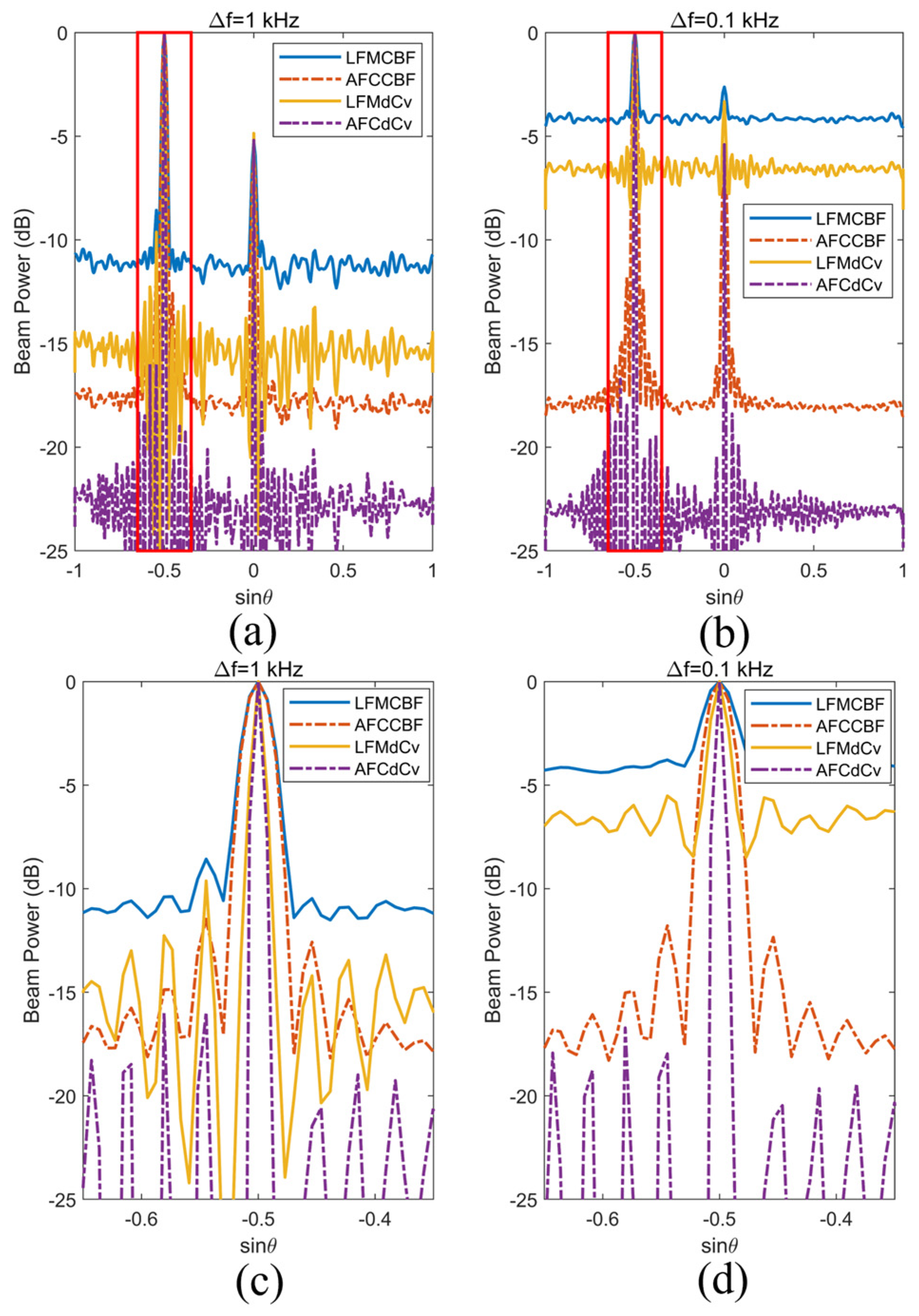
Figure 8a,b illustrate that, under sub-band intervals of 1 kHz and 0.1 kHz, the application of deconvolution processing significantly enhances both imaging resolution and sidelobe suppression for LFM and AFC signals. Regardless of whether CBF or deconvolution-based CBF is employed, the half-power width of the main lobe of AFC signals is consistently narrower than that of LFM signals, and their sidelobe suppression is markedly superior, indicating higher angular resolution, as shown in Figure 8c,d.
As the number of sub-bands increases, the main lobe becomes narrower, but this also increases the computational burden. Meanwhile, the sidelobe suppression and SNR performance of LFM signals deteriorate with increasing sub-band numbers—the sidelobe level rises by approximately 5 dB, and noise level increases by about 2 dB. In contrast, the RL deconvolved beamforming method based on AFC signals remains stable across different sub-band configurations, consistently exhibiting superior angular resolution, enhanced sidelobe suppression, and improved SNR. For instance, when the sub-band interval is set to 0.1 kHz, the sidelobe and noise levels of LFM signals after RL deconvolution are approximately −5 dB and −7 dB, respectively, whereas the corresponding values for AFC signals are −16 dB and −22 dB, further highlighting the advantages of AFC signals in high-resolution and robust imaging applications.

3.1.4. Iteration Performance

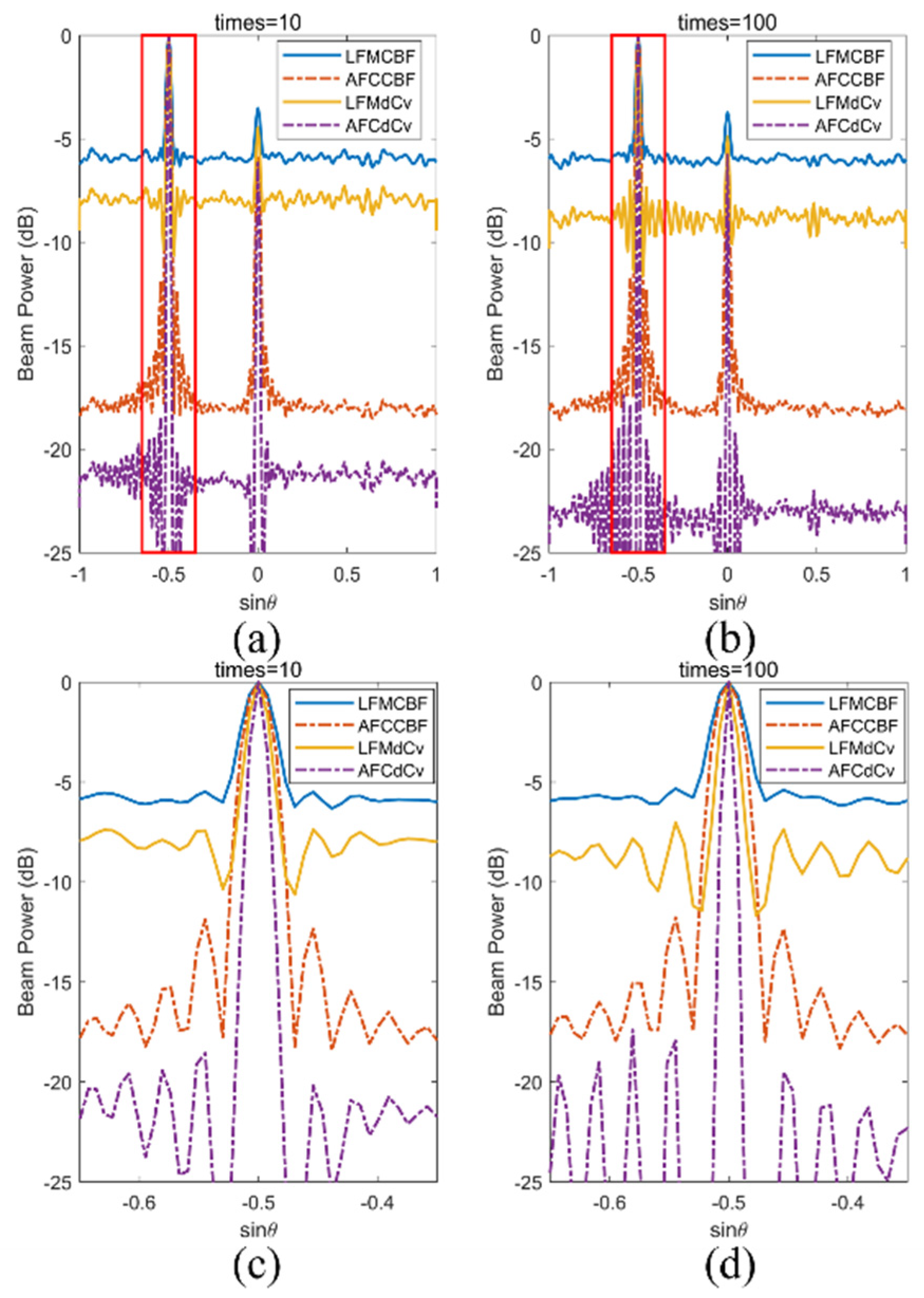
To verify the effectiveness of the AFC signal-based deconvolution method under different numbers of iterations, a comparative analysis was conducted for 10 and 100 iterations.
Figure 9a,c show that even with just 10 iterations, the deconvolution processing significantly reduces side lobes. As the number of iterations increases to 100, the main lobe width is further narrowed, while the sidelobe level and noise suppression improvement of the deconvolution method tend to stabilize, with limited additional enhancement, as shown in Figure 9c,d.
Overall, in both CBF and deconvolved CBF, AFC signals outperform LFM signals, exhibiting more rapid main lobe contraction and stronger sidelobe suppression, while consistently maintaining high angular resolution across varying numbers of iterations.

3.2. Anechoic Tank Imaging Experiment

3.2.1. Experimental Environment

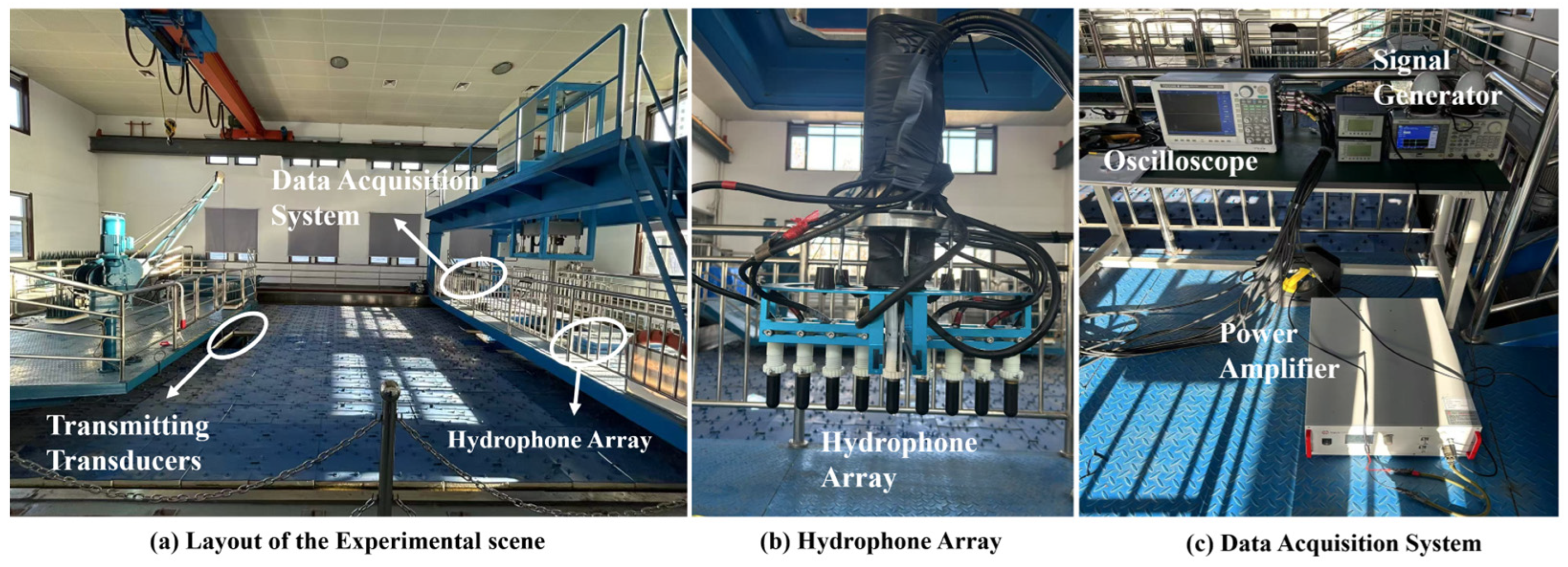
To verify the effectiveness of the deconvolved beamforming method based on AFC signals in practical applications and to compare its performance with LFM signals of equal bandwidth, this study conducted controlled experiments in the anechoic water tank at the National Marine Technology Center in Tianjin. As shown in Figure 10a, this standard large-scale indoor anechoic testing facility is approximately 15 m long, 7 m wide, and 7 m deep, with a volume of about 735 cubic meters. The walls and bottom of the tank are lined with high-efficiency sound-absorbing materials, which effectively absorb underwater sound reflections, suppress reverberation and multipath effects, and create an acoustic environment similar to a free field. A wave protection device is installed on the top of the tank to minimize interference from surface reflections.
During this experiment, the water pool maintained a stable water temperature of 20 ± 0.5 °C through a circulation system, with an acoustic speed of approximately 1485 m/s, ensuring excellent acoustic propagation stability. Additionally, the background noise level in the experimental area was kept low, which helped to improve the SNR and enhance the accuracy of the experiment. The testing system comprised two transmitting transducers, a ULA of receivers (B&K 8104), as shown in Figure 10b, and a high-precision displacement platform, designed for precise placement and reproduction of the target and array. When the signal passes through the data acquisition system (Figure 10c), measurements of two acoustic source targets at different positions were conducted to verify the high-resolution imaging capability of the proposed method in a real underwater acoustic environment.

3.2.2. Operation Process

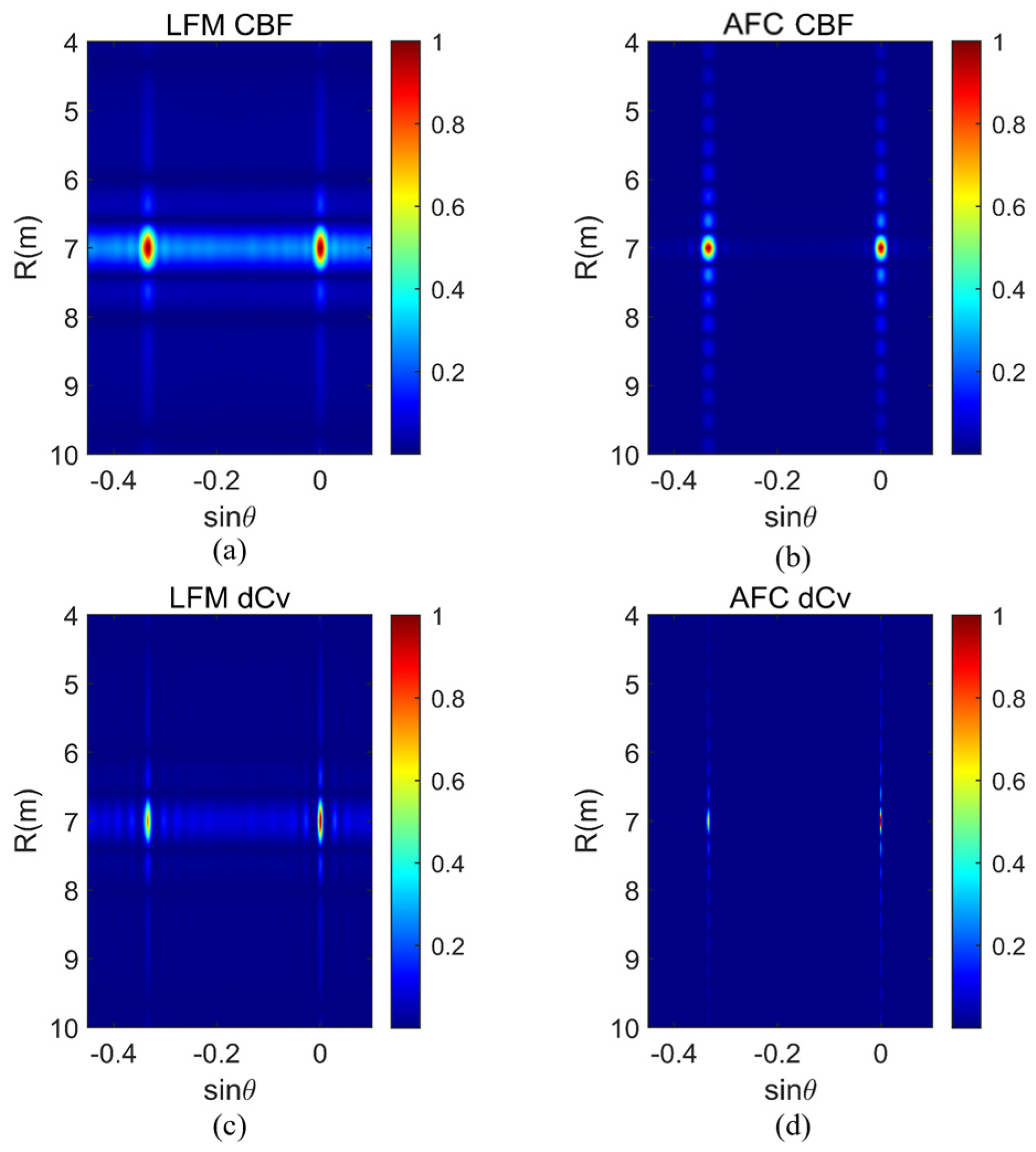
This section presents a set of experiments designed to evaluate imaging performance under multiple-target conditions. A Cartesian coordinate system is established with the center of the receiving array as the origin, and the imaging azimuth angle is set between −90° and 90°. Two targets are positioned at (7 m, 0°) and (7 m, −19.5°), respectively, using two signals with identical pulse widths and bandwidths as sources; the main parameters are detailed in Table 1. After power amplification, the signals are simultaneously transmitted through emitting transducers. The receiving array, mounted on a moving platform, collects the echo data, which is then displayed and stored using an oscilloscope. The collected data are processed separately using CBF and RL deconvolution beamforming algorithms to evaluate the imaging results.

3.2.3. Experimental Results

Figure 11a,b indicate that after CBF, the azimuth resolution of both signals is approximately equivalent. Compared to LFM signals, AFC signals exhibit higher range resolution and better sidelobe suppression.
Figure 11c,d show that after applying the RL deconvolution algorithm, the azimuthal imaging performance of both signal types is significantly enhanced. Specifically, the RL deconvolution method based on AFC signals achieves a narrower main lobe, lower sidelobe levels, and better noise suppression compared to its LFM counterpart, clearly demonstrating the high-resolution imaging capability of the AFC-RL approach.

4. Discussion

This section systematically explores the imaging performance advantages of AFC signals when combined with the RL deconvolution algorithm, focusing on four key aspects: PSF matching, frequency sparsity, autocorrelation characteristics, and computational efficiency. Compared with LFM signals of equal bandwidth, AFC signals demonstrate higher compatibility with the RL deconvolution mechanism, achieving narrower main lobes, lower sidelobe and noise levels, enhanced range resolution, and reduced computational load.
  • PSF matching: Main-lobe compression and sidelobe suppression.
AFC signals are composed of discrete, uniformly spaced narrowband frequency components:
F A F C = f 0 , f 0 + Δ f , , f 0 + K 1 Δ f .
Their sparse and regularly structured frequency distribution closely aligns with the assumptions of the PSF in deconvolution-based imaging. This structural consistency enables more accurate correction of the imaging response, resulting in narrower main lobes and effectively suppressed sidelobes. In contrast, the continuous spectrum of LFM signals introduces strong frequency-domain coupling and spectral overlap, leading to broadened main lobes and increased sidelobe energy, which degrade imaging accuracy and stability.
2.
Frequency sparsity: Lower noise level.
From the deconvolution perspective, the imaging model can be expressed as:
S ^ θ = arg m i n B θ ( S p s f ) θ 2 ,
where B is the beam output, p s f represents the system PSF, and ∗ denotes the convolution operation.
The RL deconvolution algorithm iteratively enhances signal components that match the PSF while gradually suppressing random noise that lacks structural consistency. For AFC signals, energy is concentrated at discrete frequency points, and these structured components are repeatedly reinforced during iteration, leading to stronger noise suppression. In contrast, LFM signals exhibit a continuous frequency distribution in which signal and noise are more uniformly mixed, limiting the algorithm’s ability to distinguish and eliminate noise effectively.
3.
Improved autocorrelation characteristics: Better range resolution.
AFC signals possess favorable autocorrelation properties due to their discrete and uniformly spaced frequency structure. The resulting comb-like spectrum produces a sharper and more isolated autocorrelation peak, enhancing range discrimination and resolution. LFM signals, with their continuous sweep, inherently exhibit broader autocorrelation main lobes and higher sidelobe levels, which reduce range precision and can blur adjacent targets.
4.
Lower computational complexity: Frequency discreteness and parallel processing.
In frequency-domain beamforming, the computational load depends on the number of frequency points to be processed. For LFM signals with continuous spectra, beamforming must be performed over N frequency points:
C L F M ,   B e a m f o r m i n g = M Θ N .
For AFC signals, consisting of KN discrete subcarriers, beamforming only needs to be applied to these K frequencies:
C A F C ,   B e a m f o r m i n g = M Θ K .
This discrete frequency structure allows each sub-band to be processed independently and in parallel, significantly reducing computational complexity. Meanwhile, the low coherence between sub-bands minimizes frequency coupling and maintains high imaging fidelity, making AFC signals particularly suitable for real-time, high-resolution wideband underwater imaging.

5. Conclusions

This paper presents a deconvolution beamforming method for underwater imaging based on AFC signals. The method directly addresses the problem of PSF mismatch with CBF structures that limits traditional deconvolution acceleration techniques. By taking advantage of the sparse distribution and low coherence of AFC signals in the frequency domain, these properties are incorporated into the beamforming framework, leading to significant enhancements in imaging resolution and noise suppression.
Through analysis of the PSF and the autocorrelation characteristics of AFC signals, the relevant parameters are optimized to minimize imaging artifacts. The RL algorithm serves as the primary deconvolution method, leveraging its iterative refinement and noise suppression capabilities to achieve high-resolution imaging.
Simulations demonstrate that the proposed AFC-RL method maintains robust performance even in the presence of array element errors or low SNRs. Compared with LFM-based approaches, AFC-based beamforming achieves higher resolution, enhanced sidelobe suppression, lower noise level and improved sensitivity to weak targets. Finally, controlled tank experiments validate its practical feasibility, highlighting its strong potential for advanced underwater acoustic imaging applications.

Author Contributions

Conceptualization, J.L.; methodology, J.L.; software, Y.Z.; validation, J.L.; formal analysis, J.L.; investigation, J.J.; resources, Z.Q.; data curation, J.J.; writing—original draft preparation, J.L.; writing—review and editing, D.H.; visualization, S.Y.; supervision, J.Z.; project administration, J.Z.; funding acquisition, Z.Q. All authors have read and agreed to the published version of the manuscript.

Funding

This research was funded by the Key Laboratory of Marine Environmental Survey Technology and Application, Ministry of Natural Resources, grant No. MESTA-2023-B006, National Key Research and Development Program of China, grant No. 2021YFC2803003, the Key Laboratory of Marine Environmental Information Technology, Ministry of Natural Resources, grant No. 2023E7-0081, and the State Key Laboratory of Acoustics and Marine Information, Chinese Academy of Sciences, grant No. SKLA202407.

Data Availability Statement

The raw data supporting the conclusions of this article will be made available by the authors on request.

Acknowledgments

We would like to thank the Key Laboratory of Marine Environmental Survey Technology and Application, National Key Research and Development Program of China, the Key Laboratory of Marine Environmental Information Technology, and the State Key Laboratory of Acoustics and Marine Information for their financial support during this research.

Conflicts of Interest

The authors declare no conflicts of interest.

Abbreviations

The following abbreviations are used in this manuscript:
AFCAcoustic Frequency Comb
CBFConventional Beamforming
MVDRMinimum Variance Distortionless Response
MUSICMultiple Signal Classification
ESPRITEstimation of Signal Parameters via Rotational Invariance Techniques
SNRSignal-to-Noise Ratio
DAMASDeconvolution Approach for the Mapping of Acoustic Sources
NNLSNon-Negative Least Squares
RLRichardson–Lucy
PSFPoint Spread Function
FFTFast Fourier Transform
LFMLinear Frequency Modulated
STFTShort-Time Fourier Transform

References

  1. Cong, W.; Zhou, L. Three dimensional acoustic imaging technology of buried object detection. In MATEC Web of Conferences, Proceedings of the 2nd Franco-Chinese Acoustic Conference (FCAC 2018), Les Ulis, France, 28 June 2019; Édition Diffusion Presse Sciences: Les Ulis, France, 2019; Volume 283, p. 04010. [Google Scholar]
  2. Pecknold, S.P.; Renaud, W.M.; McGaughey, D.R.; Theriault, J.A.; Marsden, R.F. Improved active sonar performance using Costas waveforms. Inst. Electr. Electron. Eng. J. Ocean. Eng. 2009, 34, 559–574. [Google Scholar] [CrossRef]
  3. Maccarone, A.; Mattioli Della Rocca, F.; McCarthy, A.; Henderson, R.; Buller, G.S. Three-dimensional imaging of stationary and moving targets in turbid underwater environments using a single-photon detector array. Opt. Express 2019, 27, 28437–28456. [Google Scholar] [CrossRef]
  4. Yang, Z.W.; Zhao, J.H.; Yu, Y.C.; Huang, C.; Yang, Z.W. A sample augmentation method for side-scan sonar full-class images that can be used for detection and segmentation. Inst. Electr. Electron. Eng. Trans. Geosci. Remote Sens. 2024, 62, 5908111. [Google Scholar] [CrossRef]
  5. Su, J.Y.; Qian, J.Y.; Tu, X.B.; Qu, F.Z.; Wei, Y. Analysis and Compensation of Acoustic Rolling Shutter Effect of Acoustic-Lens-Based Forward-Looking Sonar. Inst. Electr. Electron. Eng. J. Ocean. Eng. 2024, 49, 474–486. [Google Scholar] [CrossRef]
  6. Yang, H.L.; Zhang, S.; Tang, J.S. Study on simulation of multiple-receiver synthetic aperture sonar imagery based on wide swath. J. Syst. Simul. 2011, 23, 1424–1428. [Google Scholar]
  7. Maki, T.; Horimoto, H.; Ishihara, T.; Kofuji, K. Tracking a sea turtle by an AUV with a multibeam imaging sonar: Toward robotic observation of marine life. Int. J. Control Autom. Syst. 2020, 18, 597–604. [Google Scholar] [CrossRef]
  8. Li, J.; Stoica, P.; Wang, Z. Doubly constrained robust Capon beamformer. Inst. Electr. Electron. Eng. Trans. Signal Process 2004, 52, 2407–2423. [Google Scholar] [CrossRef]
  9. Yang, T.C. Performance analysis of superdirectivity of circular arrays and implications for sonar systems. Inst. Electr. Electron. Eng. J. Ocean. Eng. 2019, 44, 156–166. [Google Scholar] [CrossRef]
  10. Blomberg, A.E.A.; Austeng, A.; Hansen, R.E.; Synnes, S.A.V. Improving sonar performance in shallow water using adaptive beamforming. Inst. Electr. Electron. Eng. J. Ocean. Eng. 2013, 38, 297–307. [Google Scholar]
  11. Capon, J. High-resolution frequency-wavenumber spectrum analysis. Proc. Inst. Electr. Electron. Eng. 2005, 57, 1408–1418. [Google Scholar] [CrossRef]
  12. Schmidt, R. Multiple emitter location and signal parameter estimation. Inst. Electr. Electron. Eng. Trans. Antennas Propag. 1986, 34, 276–280. [Google Scholar] [CrossRef]
  13. Roy, R.; Kailath, T. ESPRIT-estimation of signal parameters via rotational invariance techniques. Inst. Electr. Electron. Eng. Trans. Acoust. Speech Signal Process. 2002, 37, 984–995. [Google Scholar]
  14. Brooks, T.F.; Humphreys, W.M. A deconvolution approach for the mapping of acoustic sources (DAMAS) determined from phased microphone arrays. J. Sound Vib. 2006, 294, 856–879. [Google Scholar] [CrossRef]
  15. Sun, D.; Ma, C.; Yang, T.C.; Mei, J.; Shi, W. Improving the performance of a vector sensor line array by deconvolution. Inst. Electr. Electron. Eng. J. Ocean. Eng. 2019, 45, 1063–1077. [Google Scholar] [CrossRef]
  16. Yang, T.C. Deconvolved conventional beamforming for a horizontal line array. Inst. Electr. Electron. Eng. J. Ocean. Eng. 2018, 43, 160–172. [Google Scholar] [CrossRef]
  17. Dougherty, R.P.; Ramachandran, R.C.; Raman, G. Deconvolution of sources in aeroacoustic images from phased microphone arrays using linear programming. Int. J. Aeroacoustics 2013, 12, 699–717. [Google Scholar] [CrossRef]
  18. Ehrenfried, K.; Koop, L. Comparison of iterative deconvolution algorithms for the mapping of acoustic sources. Am. Inst. Aeronaut. Astronaut. J. 2007, 45, 1584–1595. [Google Scholar] [CrossRef]
  19. Yardibi, T.; Li, J.; Stoica, P.; Cattafesta, L.N. Sparsity constrained deconvolution approaches for acoustic source mapping. J. Acoust. Soc. Am. 2008, 123, 2631–2642. [Google Scholar] [CrossRef] [PubMed]
  20. Wei, M.A.; Liu, X. Improving the efficiency of DAMAS for sound source localization via wavelet compression computational grid. J. Sound Vib. 2017, 395, 341–353. [Google Scholar] [CrossRef]
  21. Shen, L.; Chu, Z.; Yang, Y.; Wang, G. Periodic boundary based FFT-FISTA for sound source identification. Appl. Acoust. 2018, 130, 87–91. [Google Scholar] [CrossRef]
  22. Wu, H.; Qian, Z.; Zhang, H.; Xu, X.; Xue, B.; Zhai, J. Precise underwater distance measurement by dual acoustic frequency combs. Ann. Phys. 2019, 531, 1900283. [Google Scholar] [CrossRef]
  23. Qian, Z.; Sun, W.; Ma, X.; Han, G.; Fu, X.; Zhai, J. Quadrature acoustic frequency combs multiplexing for massive parallel underwater acoustic communications. Ann. Phys. 2022, 534, 2100426. [Google Scholar] [CrossRef]
  24. Guo, H.; Qian, Z.; Wang, X.; Sun, W.; Jie, L.; Zhai, J. A robust attitude estimation algorithm for seabed inverted ultra-short baseline. Ocean Eng. 2023, 280, 114534. [Google Scholar] [CrossRef]
  25. Li, J.; Qian, Z.; Hong, D.; Zhai, J. Precise and low-complexity method for underwater Doppler estimation based on acoustic frequency comb waveforms. Front. Mar. Sci. 2024, 11, 1365095. [Google Scholar] [CrossRef]
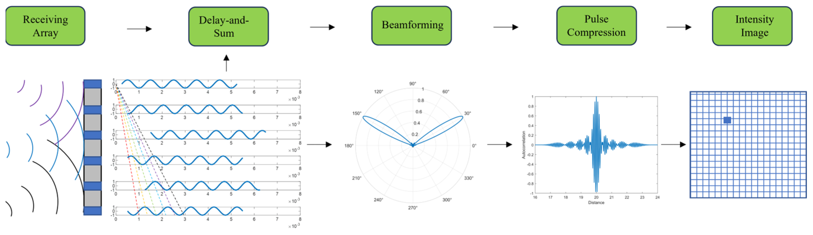
Figure 1. Working principle of multi-beam imaging sonar.
Jmse 13 02290 g001
Figure 2. Directivity functions under different parameters: (a) Relationship between directivity function and angle; (b) Directivity functions at angles of −30°, −20°, and −10°; (c) Relationship between directivity function and frequency; (d) Directivity functions at frequencies of 4 kHz, 8 kHz, and 16 kHz.
Jmse 13 02290 g002
Figure 3. Two-dimensional range-azimuth imaging results of different methods: (a) CBF; (b) RL; (c) DAMAS; (d) NNLS.
Jmse 13 02290 g003
Figure 4. Comparison of main lobe widths after pulse compression: (a) LFM pulse compression; (b) AFC pulse compression; (c) Zoomed-in view of the region highlighted in (a); (d) Zoomed-in view of the region highlighted in (b).
Jmse 13 02290 g004
Figure 5. Spectrum and autocorrelation function of signals with different snapshot lengths: (a,c,e) correspond to the Short-Time Fourier Transform (STFT) spectra for snapshots of 320, 80, and 40, respectively; (b,d,f) correspond to the autocorrelation functions for snapshots of 320, 80, and 40, respectively.
Jmse 13 02290 g005
Figure 6. Impact of array element position errors on beamforming performance: (a) CBF and deconvolved CBF results of the AFC signal under ideal (error-free) array configuration; (b) CBF and deconvolved CBF results of the AFC signal with array position errors; (c) Comparison of ideal and perturbed array element layouts.
Jmse 13 02290 g006
Figure 7. Comparison of CBF and deconvolved CBF results under different SNR conditions: (a) Comparison of CBF and deconvolved CBF for LFM and AFC signals at −10 dB SNR; (b) Comparison of CBF and deconvolved CBF for LFM and AFC signals at 0 dB SNR; (c) Zoomed-in view of the highlighted region in (a); (d) Zoomed-in view of the highlighted region in (b).
Jmse 13 02290 g007
Figure 8. CBF and deconvolved CBF under different sub-band configuration: (a) CBF and deconvolved CBF results for LFM and AFC signals with 1 kHz frequency spacing; (b) CBF and deconvolved CBF results for LFM and AFC signals with 0.1 kHz frequency spacing; (c) Zoomed-in view of the highlighted region in (a); (d) Zoomed-in view of the highlighted region in (b).
Jmse 13 02290 g008
Figure 9. Comparison of CBF and deconvolved CBF under different iteration numbers: (a) CBF and deconvolved CBF results for LFM and AFC signals with 10 iterations; (b) CBF and deconvolved CBF results for LFM and AFC signals with 100 iterations; (c) Zoomed-in view of the highlighted region in (a); (d) Zoomed-in view of the highlighted region in (b).
Jmse 13 02290 g009
Figure 10. Overall experimental setup: (a) Laboratory layout and its components; (b) Hydrophone array; (c) Data acquisition system.
Jmse 13 02290 g010
Figure 11. Comparison of imaging results. (a) CBF using LFM signal; (b) CBF using AFC signal; (c) RL deconvolution beamforming using LFM signal; (d) RL deconvolution beamforming using AFC signal.
Jmse 13 02290 g011
Table 1. Main parameters of sonar imaging.
ParameterNumeric Value
Number of elements9
Signal center frequency14 kHz
Signal bandwidth4 kHz
Signal duration2.5 ms
Frequency spacing0.2 kHz
Array Spacing4.6 cm
Disclaimer/Publisher’s Note: The statements, opinions and data contained in all publications are solely those of the individual author(s) and contributor(s) and not of MDPI and/or the editor(s). MDPI and/or the editor(s) disclaim responsibility for any injury to people or property resulting from any ideas, methods, instructions or products referred to in the content.