Article

Elemental Composition and Morphometry of Rhyssoplax olivacea (Polyplacophora): Part II—Intraspecific Variation

by
Konstantinos Voulgaris
1,
Anastasios Varkoulis
1,*,
Thomas Mygdalias
1,
Stefanos Zaoutsos
2 and
Dimitris Vafidis
1
1
Department of Ichthyology and Aquatic Environment, University of Thessaly, 38445 Volos, Greece
2
Department of Energy Systems, University of Thessaly, 41334 Larisa, Greece
*
Author to whom correspondence should be addressed.
J. Mar. Sci. Eng. 2024, 12(12), 2230; https://doi.org/10.3390/jmse12122230
Submission received: 5 November 2024 / Revised: 2 December 2024 / Accepted: 3 December 2024 / Published: 5 December 2024
(This article belongs to the Special Issue Marine Biota Distribution and Biodiversity)

Abstract

:
Rhyssoplax olivacea is a common mediterranean chiton that exhibits great geographic distribution characterized by variability in its abiotic parameters. Using morphometric measurements of the valves and radula, as well as the element composition of its tooth types from individuals sampled from five different regions across the Hellenic seas, intraspecific differences were examined. The relationship between the abiotic factors and elemental composition was also investigated. Hierarchical clustering on principal components (HCPC) was employed separately on the radular and valve characteristics to determine whether these traits can distinguish regions in the form of clusters, while canonical correspondence analysis (CCA) with ANOVA testing were used to examine the effect of temperature, depth and salinity on these features. Both datasets resulted in three clusters; however, investigation of the radula appeared to better distinguish populations among the examined regions, differentiating Kymi and Pagasitikos. The morphometrics of the valves distinguished the North Aegean Sea (Chalkidiki) from the other regions. The CCA reported that the depth, minimum temperature and average salinity influenced the elemental composition of the radular teeth, while the depth and maximum temperature explained variation regarding the valve morphometrics.

1. Introduction

Polyplacophoran mollusks (chitons) have been characterized as “living fossils” in that they have not significantly altered their morphology since the Carboniferous period [1]. The most important taxonomical characters for this taxon are the eight dorsally located valves and the radula. The size and shape of the valves are important functional traits, aiding mainly in protection from predators [2]. The radula, located in the buccal cavity, is the main component used for feeding by grazing hard surfaces [3]. Great morphological variation has been observed regarding the chiton radula, which correlates with various feeding types, ranging from detritivores and herbivores to carnivores and predators, or even with extreme specialists such as spongivorous and xylophagous species [4]. Each of these feeding types exhibit distinct radular features such as the degree of mineralization of the teeth or the relative size of the radula. The chiton valves are primarily composed of aragonite, while their radula teeth, predominantly the major tooth, contain varying amounts of magnetite [5,6].
Intraspecific differences in functional traits such as the shape and size of chiton valves or the elemental composition of the radular teeth are generally considered ecological adaptations, which allow organisms to inhabit a variety of different environments [7]. Chiton body size appears to conjure to Bergman’s rule, with larger individuals found at higher latitudes, where temperatures are lower [8]. Notably, not much does not regard either the chemical or morphometric variation in the chiton radula within the species level.
Rhyssoplax olivacea is one of the most common chiton species throughout the Mediterranean Sea; however, not much outside its distribution and population dynamics is known, mainly due to their virtually non-existent commercial significance [9,10,11]. Generally found at midlittoral boulder fields, this species can potentially affect the state of midlittoral sessile communities, when it occurs in high densities, due to increased grazing pressure (authors’ observations). R. olivacea might be directly and indirectly susceptible to future climate change. Indirect influences include climate change-induced weather events, as was shown in the central Aegean in September 2023, where the population of R. olivacea decreased to less than 20% of its original size [12]. Ocean acidification and warming can also have negative consequences for organisms with aragonite shells, such as R. olivacea [13].
Determining the variability of certain traits within the species level can help predict organismal responses to environmental changes. The present study employs multivariate techniques to examine regional differences regarding the elemental composition of the radula combined with morphometrics of both radula and valves. The influence of depth, temperature and salinity on these features are also investigated.

2. Materials and Methods

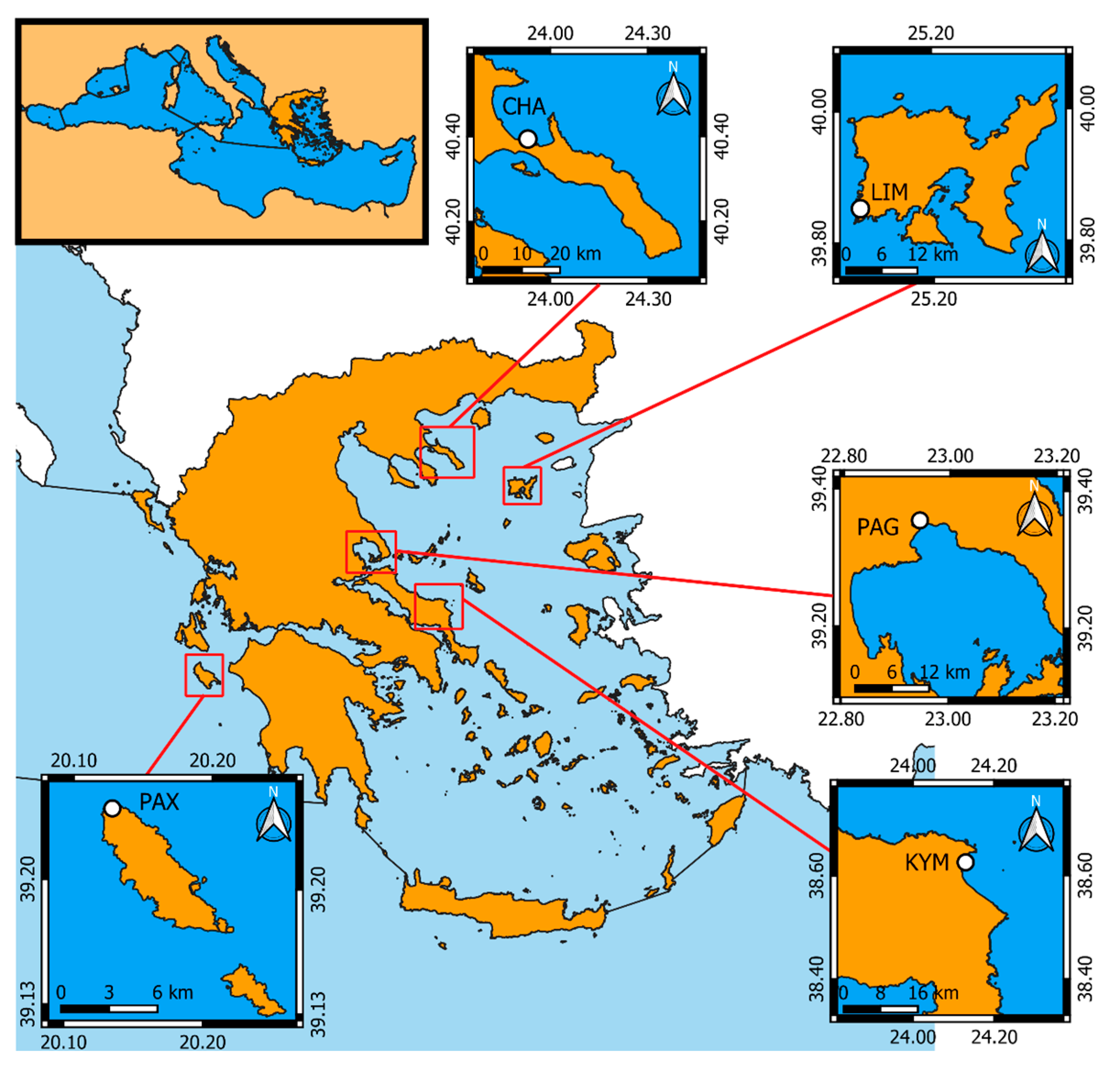
2.1. Data Collection

For the analyses, data regarding the elemental composition of the four radula tooth types and the relative radula length, as well as the morphometrics of the head and the fourth intermediate and terminal valves, were used (Table 1). The methods for data acquisition, including the use of energy-dispersive spectroscopy (EDS) and morphometric measurements, were identical to those described in detail in Part I of this series [14]. The sampled regions are shown in Figure 1. For a comprehensive description of the experimental procedures and study sites, please refer to the Methods section of Part I [14]. After a preliminary examination of the raw data, it was determined that the elemental profile of the valves remained constant among regions and thus was excluded from the analyses. Radular calcium was also removed as it contributed to little variation.
Monthly averages for the temperature and salinity were used to calculate the annual min., max. and average values by utilizing the Multi Observation Global Ocean Sea Surface Salinity and Sea Surface Density (product name: “MULTIOBS_GLO_PHY_S_SURFACE_MYNRT_015_013”) and Copernicus’ Marine Global Reanalysis (product name: “GLOBAL_MULTIYEAR_PHY_001_030”) datasets for the year 2023, respectively. The first dataset was created with a 1/8° spatial resolution. The product was obtained through a multi-dimensional (multivariate) optimal interpolation (OI) algorithm that combines sea surface salinity images from multiple satellite sources, with in situ salinity measurements and satellite sea surface temperature information [15,16,17]. The second dataset had a 1/12° spatial resolution, with the parameters being interpolated from the native grid model, the 1/12 degree and 50 vertical levels Arakawa C native grid.

2.2. Statistical Analysis

A multivariate approach was adopted by employing hierarchical clustering on principal components (HCPC). HCPC first reduces the dimensionality of the original data via principal components analysis (PCA) and subsequently uses two unsupervised machine learning techniques, namely hierarchical clustering, which groups observations together based on the scores of the retained principal components (PCs) and k-means. After the consolidation phase by k-means, the cluster assignments are refined by minimizing the within-cluster variance [18]. Data regarding the radula and valves were used independently following the same routine. To determine the number of PCs to retain, the elbow method was used. Prior to the analyses, the data were z-score-transformed. To examine the association of the variables and PCs with individual clusters, the v-test was used. Positive values indicated that a variable’s mean in the cluster was significantly higher than the overall mean, while negative values suggested the reverse.
To examine the effect of depth, temperature and salinity, canonical correspondence analysis was employed separately for the radular and valve features. This method was used because it can effectively describe both the unimodal and linear relationships of a response matrix along environmental gradients [19]. The minimum, maximum and mean temperature and salinity, as well as the depth, were used as constraint covariates. Before the analysis predictors were examined for multicollinearity using the (VIF), stepwise forward selection was conducted to determine the most important factors to include in the model. The statistical effect was examined from sequential tests with the function “anova.cca”, a permutational ANOVA-like test, with the number of permutations set at 999.
All statistical analyses were conducted using the R language in the RStudio (version 2024.09.0+375) programming environment. The package factoMiner was used for the HCPC analysis, while the package vegan was used for CCA [20,21].

3. Results

3.1. Radular Elemental Composition and Morphometry

The first two PCs were used for the HCPC, explaining a total variance of 52.3% (PC1: 35.6%; PC2: 16.7%). The highest contribution was reported for KL1 in PC1 and for MgL1 in PC2, while FeL1, PL1, SiM, SiL1 and SiC showed high contributions in both PCs (Figure 2). Most variables were adequately represented by the combination of the two PCs except for SiL2, MgM, FeM and FeC (Figure 2). All variables exhibited moderate to strong positive or negative correlations with at least one PC, except for FeC, MgM and SiL2 (Figure 2).
Based on the HCPC, three clusters were produced, with most of the individuals from Kymi belonging to the first cluster, while most of those from Pagasitikos and Chalkidiki being placed in the second and third clusters, respectively (Figure 3). Observations from Limnos and Paxos were mostly grouped together in the third cluster, with only three individuals from each region belonging to the second cluster (Figure 3). SiL1, SiM and SiC exhibited the highest positive association, whereas PC, PL2, KL1, KM and PM showed a strong negative association with cluster 1. For cluster 2, positive associations for FeL1 and FeM were reported, while MgL2 and MgL1 were negatively associated with this cluster. PC, PL1, MgL2, KL1, PL2, KC, MgL1 and PM were positively represented, whereas FeM, STRL and FeL1 were negatively represented in cluster 3 (Table 2). PC1 showed a negative association with cluster 1 and a positive association with cluster 3, while PC2 exhibited a positive association with cluster 1 and a negative association with cluster 2 (Table 2).

3.2. Valve Morphometrics

Overall, the first two PCs explained most of the total variation (PC1: 60.5%; PC2: 12%) regarding the morphometrics of the valves. Except for the standardized thickness of the valves (STIT, STIVT, STVIIIT), all other variables significantly contributed to the first PC, with the STIVW showing the largest contribution (Figure 4). As for the second PC, the STVIIIT showed the highest contribution, followed by the STIT and STVIIIL (Figure 4). All included variables were well represented by the combination of the first two PCs, while also exhibiting high- and weak-to-moderate correlations with PC1 and PC2, respectively, except for the STVIIIT, which presented the highest correlation with PC2 (Figure 4).
The HCPC grouped observations in three clusters, with cluster 1 containing all individuals from Paxos and cluster 3 including the majority of specimen derived from Chalkidiki (Figure 5). Individuals from Limnos, Pagasitikos and Kymi were mostly clustered either in cluster 1 or 2, without exhibiting any distinct trend (Figure 5). All variables were negatively represented in cluster 1 and positively represented in cluster 3, with the lowest and highest values being observed for the STIW for the former and the latter, respectively (Table 3). There were no variables significantly distinguishing the second cluster. Regarding the association of the PCs and clusters, PC1 was negatively and positively represented in clusters 1 and 3, respectively (Table 3).

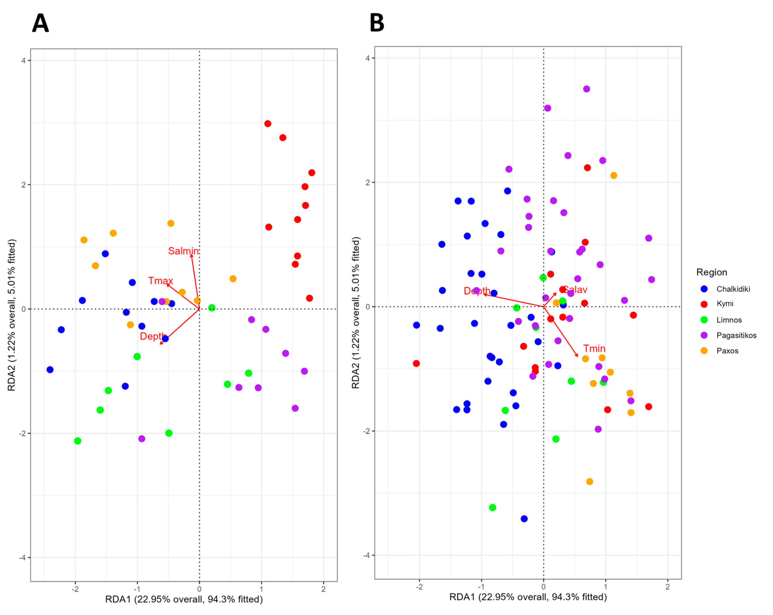
3.3. Influence of Abiotic Variables

After checking for multicollinearity and conducting stepwise forward selection, the remaining variables that best explained the variation regarding the radular traits included Tmax, Salmin and Depth. The first two CCAs combined explained 84.5% of the fitted and 14.9% of the total variation. Permutation tests ran for the full model, axes and constraints reported that the model was significant, with the first two CCAs showing statistical importance and that all abiotic covariates were significant predictors (Table 4). Depth and Tmax were negatively associated with the CCA1 (−0.52 and −0.63, respectively), while the CCA2 was positively associated with Salmin and negatively correlated to Depth (0.88 and −0.56, respectively). Depth and Tmax separated individuals sampled from Chalkidiki, Paxos and Limnos from those belonging to Kymi and Pagasitikos in the CCA1, while Salmin distinguished Limnos and Pagasitikos from Kymi in the CCA2 (Figure 6).
The final set of environmental predictors best explaining the variation regarding the morphometrics of the valves of R. olivacea included Tmin, Depth and Salav, with the first two CCAs explaining 99.31% of the fitted and 24.17% of the total variance. Although the full model was statistically important, only the first CCA exhibited significance, while Salav showed no statistical effect (Table 4). Depth presented a strong negative association whereas Tmin presented positive association to CCA1 (−0.96 and 0.55, respectively). No clear trend can be observed except for the separation between individuals from Chalkidiki and Paxos, with the former being located towards an increasing depth and the latter towards an increased Tmin, occupying opposite positions along the CCA1 (Figure 6).

4. Discussion

Variation in the relative length of the radular and the elemental composition of the teeth seems to be influenced mainly by feeding preferences at the species level [4,6]. Changes in the relative size of the feeding apparatus have been linked to food availability (e.g., a larger Aristotle’s lantern related to food scarcity; [22]). Cluster 3, which included observations from the North Aegean and Ionian Seas, exhibited lower relative radular lengths compared to those from Central Aegean specimens belonging to the Central Aegean (Pagasitikos and Kymi) clusters, which exhibited larger radula lengths, possibly hinting at local food limitations.
This is the first study to compare the elemental composition of a molluscan radula intraspecifically. Differences in concentrations of elements across the different tooth types showed a significant variation at the population level, with specimen from the Central Aegean forming two distinct clusters, while those from North Aegean and Ionian Seas being clustered together. The importance and function of the lateral II tooth has been extensively studied. The specific motion patterns coupled with specific mechanical properties of this tooth appear to enable mollusks and specifically chitons to acquire food from hard substrates [6]. These mechanical properties are heavily influenced by iron concentration in the lateral II tooth, conferring increased hardness, a trend not distinctly observed for the other three tooth types [6,23,24,25,26]. FeL2 was not significantly associated with any of the clusters, indicating that FeL2 specifically might be directly related to evolutionary phylomineralogy.
The width of the fourth valve of Sypharochiton pelliserpentis was shown to decrease with increasing wave action [27]. The circularity and height of the fourth valve, the width of the head valve, and the height of the tail valve have been found to be highly variable among 16 populations of Onithochiton neglectus across New Zealand, suggesting that valve shape and size can be considered an adaptive trait [28]. Shell thickness is correlated to increased protection against predation at the expense of growth in marine gastropods [29]. Here, individuals belonging to cluster 3 (Chalkidiki) exhibited the highest valve thickness and lowest body length [14]. Given that predation pressure for marine mollusks increases from the midlittoral towards the sublittoral zone, the observed increase in the valve thickness with depth was probably an adaptation to increased predation pressure [30].
Abiotic factors are the main influence on intraspecific variation for marine invertebrates. Tooth Mg/Ca in echinoids both native and invasive to the Mediterranean has been shown to change with temperature [31]. Marine mollusks exhibit different responses related to environmental changes regarding their shells, which are dependent on metabolic demands and food availability [32,33]. Decreased salinity seems to have a negative influence on shell thickness; thus, it is considered an adaptive trait [34]. Wave action also seems to influence valve thickness and width in chitons [2,27]. For R. olivacea, temperature, salinity and depth seem to have a combining effect on elemental composition variability at a regional scale, while salinity does not appear to affect the valve morphometry. In terms of radular traits, an increased minimum salinity seems to affect the concentrations of predominantly Si, P and K, while a decreased maximum salinity might influence Fe and Mg concentrations.
The relationship between temperature and mollusk shell size is complex, with contrasting results even for the same species [35]. Energetic trade-offs between metabolic demands and energy acquisition appear to affect the rate of energy allocation to the shell [36]. An increased minimum temperature possibly reduces the thickness of all valves, while individuals collected from an increased depth showed higher values for all morphological valve traits. This might indicate that R. olivacea might be directly influenced by future ocean warming, due to the synergetic effect of a thin and weak shell and increased metabolic demands; however, this hypothesis remains to be tested.
The present study suggests that not only morphometry but also elemental composition could function as an ecological adaptation in marine mollusks, as shown here for R. olivacea, while the influence of local environmental factors should also be considered. The effects of wave action, feeding preferences and predation were not investigated; thus, the focus of future research should be to extend our knowledge regarding the influence of local environmental regimes and biotic interactions on intraspecific morphometric and elemental variation in chitons.

Author Contributions

Conceptualization A.V., K.V. and D.V.; methodology A.V., K.V., T.M. and S.Z.; formal analysis A.V., K.V., T.M. and D.V.; project administration D.V.; supervision D.V.; visualization A.V., K.V. and D.V.; writing—original draft A.V., T.M. and K.V.; writing—review and editing A.V., K.V., T.M. and D.V. All authors have read and agreed to the published version of the manuscript.

Funding

This research received no external funding.

Institutional Review Board Statement

No ethical issues related with the use of animals in the laboratory procedures were involved.

Informed Consent Statement

Not applicable.

Data Availability Statement

The raw data supporting the conclusions of this article will be made available by the authors on request.

Conflicts of Interest

The authors declare no conflicts of interest.

References

  1. Sirenko, B. New Outlook on the System of Chitons (Mollusca: Polyplacophora). Venus 2006, 65, 27–49. [Google Scholar]
  2. Sigwart, J.D.; Green, P.A.; Crofts, S.B. Functional Morphology in Chitons (Mollusca, Polyplacophora): Influences of Environment and Ocean Acidification. Mar. Biol. 2015, 162, 2257–2264. [Google Scholar] [CrossRef]
  3. Scheel, C.; Gorb, S.N.; Glaubrecht, M.; Krings, W. Not Just Scratching the Surface: Distinct Radular Motion Patterns in Mollusca. Biol. Open 2020, 9, bio055699. [Google Scholar] [CrossRef]
  4. Sigwart, J.D.; Schwabe, E. Anatomy of the Many Feeding Types in Polyplacophoran Molluscs. Invertebr. Zool. 2017, 14, 205–216. [Google Scholar] [CrossRef]
  5. Kirschvink, J.L.; Lowenstam, H.A. Mineralization and Magnetization of Chiton Teeth: Paleomagnetic, Sedimentologic, and Biologic Implications of Organic Magnetite. Earth Planet. Sci. Lett. 1979, 44, 193–204. [Google Scholar] [CrossRef]
  6. Krings, W.; Brütt, J.-O.; Gorb, S.N. Elemental Analyses Reveal Distinct Mineralization Patterns in Radular Teeth of Various Molluscan Taxa. Sci. Rep. 2022, 12, 7499. [Google Scholar] [CrossRef]
  7. Paaby, A.B.; Testa, N.D. Developmental Plasticity and Evolution. In Evolutionary Developmental Biology: A Reference Guide; Nuño de la Rosa, L., Müller, G.B., Eds.; Springer International Publishing: Cham, Switzerland, 2021; pp. 1073–1086. ISBN 978-3-319-32979-6. [Google Scholar]
  8. Hernández-P, R.; Benítez, H.A.; Ornelas-García, C.P.; Correa, M.; Suazo, M.J.; Piñero, D. Bergmann’s Rule under Rocks: Testing the Influence of Latitude and Temperature on a Chiton from Mexican Marine Ecoregions. Biology 2023, 12, 766. [Google Scholar] [CrossRef]
  9. Dell’Angelo, B.; Smriglio, C. Living Chitons of the Mediterranean; Evolver: Rome, Italy, 2001; ISBN 978-88-8299-007-7. [Google Scholar]
  10. Koukouras, A.; Karachle, P. The Polyplacophoran (Eumollusca, Mollusca) Fauna of the Aegean Sea with the Description of a New Species, and Comparison with Those of the Neighbouring Seas. J. Biol. Res. 2004, 3, 23–38. [Google Scholar]
  11. Varkoulis, A.; Voulgaris, K.; Zachos, D.S.; Vafidis, D. Population Dynamics of Three Polyplacophora Species from the Aegean Sea (Eastern Mediterranean). Diversity 2023, 15, 867. [Google Scholar] [CrossRef]
  12. Mygdalias, T.; Voulgaris, K.; Varkoulis, A.; Zachos, D.S.; Vafidis, D. Short-Term Effect of Extreme Storms on Population Characteristics of a Common Mediterranean Chiton. In Proceedings of the HydroMediT 2024, Mytilene, Greece, 30 May–2 June 2024; p. 4. [Google Scholar]
  13. Intergouvernemental Panel on Climate Change (Ed.) Climate Change 2007: The Physical Science Basis; Cambridge University Press: Cambridge, UK, 2007; ISBN 978-0-521-88009-1. [Google Scholar]
  14. Mygdalias, T.; Varkoulis, A.; Voulgaris, K.; Zaoutsos, S.; Vafidis, D. Elemental Composition and Morphometry of Rhyssoplax olivacea (Polyplacophora): Part I—Radula and Valves. J. Mar. Sci. Eng. 2024, 12, 2186. [Google Scholar] [CrossRef]
  15. Nardelli, B.B. A Novel Approach for the High-Resolution Interpolation of In Situ Sea Surface Salinity. J. Atmos. Ocean. Technol. 2012, 29, 867–879. [Google Scholar] [CrossRef]
  16. Buongiorno Nardelli, B.; Droghei, R.; Santoleri, R. Multi-Dimensional Interpolation of SMOS Sea Surface Salinity with Surface Temperature and in Situ Salinity Data. Remote Sens. Environ. 2016, 180, 392–402. [Google Scholar] [CrossRef]
  17. Droghei, R.; Buongiorno Nardelli, B.; Santoleri, R. A New Global Sea Surface Salinity and Density Dataset from Multivariate Observations (1993–2016). Front. Mar. Sci. 2018, 5, 84. [Google Scholar] [CrossRef]
  18. Husson, F.; Le, S.; Pagès, J. Exploratory Multivariate Analysis by Example Using R; CRC Press: Boca Raton, FL, USA, 2010; ISBN 978-0-429-19003-2. [Google Scholar]
  19. Ter Braak, C.J.F. The Analysis of Vegetation-Environment Relationships by Canonical Correspondence Analysis. Vegetatio 1987, 69, 69–77. [Google Scholar] [CrossRef]
  20. Lê, S.; Josse, J.; Husson, F. FactoMineR: An R Package for Multivariate Analysis. J. Stat. Softw. 2008, 25, 1–18. [Google Scholar] [CrossRef]
  21. Oksanen, J.; Blanchet, F.G.; Kindt, R.; Legendre, P.; Minchin, P.; O’Hara, R.; Simpson, G.; Solymos, P.; Stevens, M.; Wagner, H. Vegan: Community Ecology Package, R Package Version 2.0-10; CRAN: Vienna, Austria, 2013. [Google Scholar]
  22. Black, R.; Codd, C.; Hebbert, D.; Vink, S.; Burt, J. The Functional Significance of the Relative Size of Aristotle’s Lantern in the Sea Urchin Echinometramathaei (de Blainville). J. Exp. Mar. Biol. Ecol. 1984, 77, 81–97. [Google Scholar] [CrossRef]
  23. Weaver, J.C.; Wang, Q.; Miserez, A.; Tantuccio, A.; Stromberg, R.; Bozhilov, K.N.; Maxwell, P.; Nay, R.; Heier, S.T.; DiMasi, E.; et al. Analysis of an Ultra Hard Magnetic Biomineral in Chiton Radular Teeth. Mater. Today 2010, 13, 42–52. [Google Scholar] [CrossRef]
  24. Grunenfelder, L.K.; de Obaldia, E.E.; Wang, Q.; Li, D.; Weden, B.; Salinas, C.; Wuhrer, R.; Zavattieri, P.; Kisailus, D. Stress and Damage Mitigation from Oriented Nanostructures within the Radular Teeth of Cryptochiton stelleri. Adv. Funct. Mater. 2014, 24, 6093–6104. [Google Scholar] [CrossRef]
  25. Barber, A.H.; Lu, D.; Pugno, N.M. Extreme Strength Observed in Limpet Teeth. J. R. Soc. Interface 2015, 12, 20141326. [Google Scholar] [CrossRef]
  26. Wang, Q.; Nemoto, M.; Li, D.; Weaver, J.C.; Weden, B.; Stegemeier, J.; Bozhilov, K.N.; Wood, L.R.; Milliron, G.W.; Kim, C.S.; et al. Phase Transformations and Structural Developments in the Radular Teeth of Cryptochiton stelleri. Adv. Funct. Mater. 2013, 23, 2908–2917. [Google Scholar] [CrossRef]
  27. Horn, P.L. Adaptations of the Chiton Sypharochiton pelliserpentis to Rocky and Estuarine Habitats. N. Z. J. Mar. Freshw. Res. 1982, 16, 253–261. [Google Scholar] [CrossRef]
  28. Salloum, P.M.; Santure, A.W.; Lavery, S.D.; de Villemereuil, P. Finding the Adaptive Needles in a Population-Structured Haystack: A Case Study in a New Zealand Mollusc. J. Anim. Ecol. 2022, 91, 1209–1221. [Google Scholar] [CrossRef]
  29. Palmer, A.R. Adaptive Value of Shell Variation in Thais Lamellosa: Effect of Thick Shells on Vulnerability to and Preference by Crabs. Veliger 1985, 27, 349–356. [Google Scholar]
  30. Perez, K.O.; Carlson, R.L.; Shulman, M.J.; Ellis, J.C. Why Are Intertidal Snails Rare in the Subtidal? Predation, Growth and the Vertical Distribution of Littorina littorea (L.) in the Gulf of Maine. J. Exp. Mar. Biol. Ecol. 2009, 369, 79–86. [Google Scholar] [CrossRef]
  31. Vafidis, D.; Varkoulis, A.; Zaoutsos, S.; Voulgaris, K. Tooth Mg/Ca Ratios and Aristotle’s Lantern Morphometrics Reflect Trophic Types in Echinoids. Ecol. Evol. 2024, 14, e11251. [Google Scholar] [CrossRef] [PubMed]
  32. Mackenzie, C.L.; Ormondroyd, G.A.; Curling, S.F.; Ball, R.J.; Whiteley, N.M.; Malham, S.K. Ocean Warming, More than Acidification, Reduces Shell Strength in a Commercial Shellfish Species during Food Limitation. PLoS ONE 2014, 9, e86764. [Google Scholar] [CrossRef]
  33. Fernández, C.; Poupin, M.J.; Lagos, N.A.; Broitman, B.R.; Lardies, M.A. Physiological Resilience of Intertidal Chitons in a Persistent Upwelling Coastal Region. Sci. Rep. 2024, 14, 21401. [Google Scholar] [CrossRef] [PubMed]
  34. Clark, M.S.; Peck, L.S.; Arivalagan, J.; Backeljau, T.; Berland, S.; Cardoso, J.C.R.; Caurcel, C.; Chapelle, G.; De Noia, M.; Dupont, S.; et al. Deciphering Mollusc Shell Production: The Roles of Genetic Mechanisms through to Ecology, Aquaculture and Biomimetics. Biol. Rev. 2020, 95, 1812–1837. [Google Scholar] [CrossRef]
  35. Gizzi, F.; Caccia, M.G.; Simoncini, G.A.; Mancuso, A.; Reggi, M.; Fermani, S.; Brizi, L.; Fantazzini, P.; Stagioni, M.; Falini, G.; et al. Shell Properties of Commercial Clam Chamelea Gallina Are Influenced by Temperature and Solar Radiation along a Wide Latitudinal Gradient. Sci. Rep. 2016, 6, 36420. [Google Scholar] [CrossRef]
  36. Moschino, V.; Marin, M.G. Seasonal Changes in Physiological Responses and Evaluation of “Well-Being” in the Venus Clam Chamelea gallina from the Northern Adriatic Sea. Comp. Biochem. Physiol. Part A Mol. Integr. Physiol. 2006, 145, 433–440. [Google Scholar] [CrossRef]
Figure 1. Map of Greece showing the five study areas (white circles).
Jmse 12 02230 g001
Figure 2. Principal component analysis (PCA) for the elemental composition of tooth types. (A) A biplot showing the quality of the representation of each variable by the first two PCs. (B) Bar plots showing the contribution (%) of each variable to PC1 and PC2. The red dashed line indicates the expected average contribution if all variables were to contribute equally. (C) A correlation matrix showing the correlation coefficients between each variable and the first two principal components.
Jmse 12 02230 g002
Figure 3. HCPC based on the elemental composition of the radular tooth types (A) before and (B) after consolidation with k-means. The color of each cluster is indicative of the region that had the majority of observations within the specific cluster.
Jmse 12 02230 g003
Figure 4. Principal component analysis (PCA) for the morphometric measurements of the valves and radula. (A) A biplot showing the quality of the representation of each variable by the first two PCs. (B) Bar plots showing the contribution (%) of each variable to PC1 and PC2. The red dashed line indicates the expected average contribution if all variables were to contribute equally. (C) A correlation matrix showing the correlation coefficients between each variable and the first two principal components.
Jmse 12 02230 g004
Figure 5. HCPC based on the morphometric measurements for the valves and radula (A) before and (B) after consolidation with k-means. The color of each cluster is indicative of the region that had the majority of observations within the specific cluster. A black color for cluster 2 indicates no representative region.
Jmse 12 02230 g005
Figure 6. CCA based on data for (A) the elemental composition of tooth types and (B) standardized morphometric measurements for the valves and radula. Red arrows show sets of abiotic parameters best explaining the variation for each dataset, with the arrow length being indicative of the significance of each parameter.
Jmse 12 02230 g006
Table 1. The definitions of indicators used throughout the text.
Indicator DomainsAbbreviationDescription
Elemental compositionSiL1Silicon Lateral I
SiL2Silicon Lateral II
SiMSilicon Marginal
SiCSilicon Central
PL1Phosphorus Lateral I
PL2Phosphorus Lateral II
PMPhosphorus Marginal
PCPhosphorus Central
KL1Potassium Lateral I
KL2Potassium Lateral II
KMPotassium Marginal
KCPotassium Central
FeL1Iron Lateral I
FeL2Iron Lateral II
FeMIron Marginal
FeCIron Central
MgL1Magnesium Lateral I
MgL2Magnesium Lateral II
MgMMagnesium Marginal
MgCMagnesium Central
Standardized morphometrics for head (I), intermediate (IV) and tail (VIII) valves and radulaSTILLength of I
STIWWidth of I
STITThickness of I
STIVLLength of IV
STIVWWidth of IV
STIVTThickness of IV
STVIIILLength of VIII
STVIIIWWidth of VIII
STVIIITThickness of VIII
STRLRadula Length
Regional abbreviationsCHAChalkidiki Peninsula
LIMLimnos Island
PAGPagasitikos Gulf
KYMKymi (Evoia Island)
PAXPaxos Island
Abiotic factorsDepthSampling Depth
TminMinimum Annual Temperature
TmaxMaximum Annual Temperature
SalavAverage Annual Salinity
SalminMinimum Annual Salinity
Table 2. HCPC results based on the elemental composition of radular tooth types showing the most significant associated PCs and variables for each cluster. Because the data were z-score-transformed, the results indicate the statistical significance and strength of the deviation of the mean in the cluster from the global mean.
ClustersPrincipal
Components
Variablesv.testMeanp-Value
1PC2 3.051.570.002
PC1 −4.93−3.750.000
SiL15.751.730.000
SiM5.561.680.000
SiC4.551.370.000
PC−3.02−0.910.003
PL2−3.13−0.940.002
KL1−3.14−0.950.002
KM−3.48−1.050.001
PM−3.50−1.060.000
2PC2 −4.72−1.660.000
FeL13.470.710.001
FeM3.300.680.001
MgL2−3.01−0.620.003
MgL1−3.48−0.710.001
3PC1 5.762.120.000
PC5.010.730.000
PL14.750.690.000
MgL24.530.660.000
KL14.110.600.000
PL24.080.590.000
KC3.960.580.000
MgL13.850.560.000
PM3.220.470.001
FeM−3.34−0.490.001
STRL−4.26−0.620.000
FeL1−4.40−0.640.000
Table 3. HCPC results based on the morphometric measurements for the valves and radula showing the most significant associated PCs and variables for each cluster. Because the data were z-score-transformed, the results indicate the statistical significance and strength of the deviation of the mean in the cluster from the global mean.
ClustersPrincipal
Components
Variablesv.testMeanp-Value
1PC1 −7.42−2.710.000
STVIIIT−3.30032−0.513130.001
STIVT−4.53104−0.704480.000
STIT−5.11977−0.796010.000
STVIIIL−5.68382−0.883710.000
STVIIIW−6.07251−0.944140.000
STIVL−6.07471−0.944490.000
STIL−6.61804−1.028960.000
STIVW−6.69796−1.041390.000
STIW−6.96144−1.082350.000
2
3PC1 7.732.890.000
STIW7.0442491.1227790.000
STIL6.8703691.0950650.000
STIVW6.7506481.0759820.000
STVIIIL6.3807091.0170180.000
STIVL6.1264090.9764850.000
STVIIIW5.8627770.9344650.000
STIT5.6811760.905520.000
STIVT5.0786620.8094850.000
STVIIIT3.6279330.5782540.000
Table 4. Results from permutational ANOVA-like tests for canonical correspondence analysis (CCA) for the influence of the abiotic factors on the elemental composition of the tooth types and morphometric measurements for the valves and radula. Significant differences (p < 0.05) are highlighted in bold.
ComponentElemental CompositionMorphometrics
TermFp-ValueTermFp-Value
VariablesTmax2.68610.008Tmin9.36860.001
Salmin3.55960.002Depth19.59920.001
Depth3.37530.003Salav0.95430.366
AxesCCA14.75590.002CCA128.21580.001
CCA23.37940.005CCA21.49990.421
Disclaimer/Publisher’s Note: The statements, opinions and data contained in all publications are solely those of the individual author(s) and contributor(s) and not of MDPI and/or the editor(s). MDPI and/or the editor(s) disclaim responsibility for any injury to people or property resulting from any ideas, methods, instructions or products referred to in the content.

