Retrieval of Three-Dimensional Wave Surfaces from X-Band Marine Radar Images Utilizing Enhanced Pix2Pix Model

Abstract

In this study, we propose a novel method for retrieving the three-dimensional (3D) wave surface from sea clutter using both simulated and measured data. First, the linear wave superposition model and modulation principle are employed to generate simulated datasets comprising 3D wave surfaces and corresponding sea clutter. Subsequently, we develop a Pix2Pix model enhanced with a self-attention mechanism and a multiscale discriminator to effectively capture the nonlinear relationship between the simulated 3D wave surfaces and sea clutter. The model’s performance is evaluated through error analysis, comparisons of wave number spectra, and differences in wave surface reconstructions using a dedicated test set. Finally, the trained model is applied to reconstruct wave surfaces from sea clutter data collected aboard a ship, with results benchmarked against those derived from the Schrödinger equation. The findings demonstrate that the proposed model excels in preserving high-frequency image details while ensuring precise alignment between reconstructed images. Furthermore, it achieves superior retrieval accuracy compared to traditional approaches, highlighting its potential for advancing wave surface retrieval techniques.

1. Introduction

Sea wave information is critical for a wide range of onshore and offshore activities, including ship navigation, coastal infrastructure development, and the exploration of marine resources. Therefore, obtaining accurate sea wave data is of paramount importance, particularly in the domain of ocean remote sensing [1].

A range of measurement techniques is employed to capture the physical parameters of sea waves, encompassing traditional methods such as manual observations and buoy measurements, as well as advanced technologies like spaceborne Synthetic Aperture Radar (SAR), shore-based coherent S-band radar, and navigation X-band marine radar [2,3,4,5]. Particularly, X-band marine radar has been rapidly developed as an ocean remote sensor since it can image both the spatial and temporal variations of the sea surface with high resolutions. Furthermore, X-band marine radar is widely installed on ships for navigation purposes. If reliable wave measurements can be obtained from such radars, the costs associated with buoys can be significantly reduced. Thus, ship-borne X-band marine radar has garnered wide attention.

Recently, numerous algorithms have been developed for wave measurement using X-band marine radar. These existing methods can be broadly classified into two categories: spectral-analysis-based techniques and texture-analysis-based techniques, as summarized in

Table 1. Algorithms for wave measurement using X-band marine radar.

Techniques	Methods	Reference
Spectral Analysis	3D-DFT	[6,7,8]
	2D Continuous Wavelet Transform	[9,10]
	Array Beamforming	[11]
Texture Analysis	Illumination Probability	[12,13]
	Statistical Analysis	[14,15]
	Tilt or Shadowing Analysis	[16,17]
	Data Decomposition	[18,19]
	Machine Learning	[20,21,22,23]

.

Among various approaches, machine learning has gained widespread attention due to its strong nonlinear modeling capabilities and end-to-end framework. However, existing machine learning methods are primarily applied to the retrieval of statistical parameters such as wave height and wave period and are not suitable for reconstructing the full three-dimensional wave surface. Furthermore, traditional machine learning methods, which are predominantly based on supervised learning, aim to minimize a loss function to approximate the true target. Nevertheless, the generated three-dimensional wave surfaces often suffer from blurriness or lack of detail, particularly when applied to complex scenarios [19].

Therefore, this paper proposes an enhanced Pix2Pix model incorporating an attention mechanism to effectively reconstruct 3D sea wave surfaces. Pix2Pix, based on Conditional Generative Adversarial Networks (CGAN), integrates conditional information into both the generator and discriminator, enabling a more controllable and precise 3D wave surface generation process. The attention mechanism, inspired by the selective focus capabilities of the human visual system, allows the model to concentrate on critical features when processing complex images. By integrating this mechanism, the enhanced Pix2Pix model significantly improves its ability to generate accurate 3D sea wave surfaces during retrieval while maintaining robust performance even in challenging and noisy environments.

The primary contributions of this study are as follows:

• We propose an improved Pix2Pix model incorporating an attention mechanism and a multiscale discriminator. This model leverages the strengths of Generative Adversarial Networks (GANs) to effectively process high-frequency image details and ensure precise correspondence between images. The integration of the self-attention mechanism and the multiscale discriminator enhances the network’s ability to capture and learn global features.
• Retrieval experiments are conducted on both simulated and measured datasets. The results demonstrate that the proposed model significantly outperforms traditional retrieval methods in processing high-frequency image details and preserving image correspondence accuracy, thereby achieving superior retrieval performance.

The remainder of this paper is structured as follows: Section 2 provides a comprehensive overview of the dataset construction and model development processes. Section 3 presents a detailed experimental analysis of the retrieval results. Section 4 concludes this study and discusses potential future research directions.

2. Materials and Methods

2.1. Dataset

2.1.1. 3D Wave Surface

We utilize linear wave theory to numerically simulate the three-dimensional wave surface. To achieve this, the JONSWAP (Joint North Sea Wave Project) spectrum and the Mitsuyasu directional spreading function are applied to construct a detailed three-dimensional representation of sea wave surfaces. The specific methodology is outlined as follows:

• Linear superposition model

As a stationary random process, sea waves can be represented as the superposition of multiple cosine waves, each defined by unique initial phases and varying periods. This conceptualization is mathematically expressed in Equation (1) [24]:

$$\eta \left(x,y,t\right)=\sum _{i=1}^M\sum _{j=1}^N{a}_{ij}\mathit{cos}\left({\omega }_{i}t-k_{i}x\mathit{cos}{\theta }_j-k_{i}y\mathit{cos}{\theta }_j+{\delta }_{ij}\right)$$

(1)

Here, $x$ and $y$ represent coordinates on the horizontal plane, and $\eta \left(x,y,t\right)$ denotes the wave height at the point $(x,y)$ in time $t$. The term $a_{ij}$ refers to the amplitude of the component wave with angular frequency ${\omega }_i$, propagating in a direction forming an angle ${\theta }_j$ with the $x$-axis.

The initial phase angle of each constituent wave denoted as ${\delta }_{ij}$, is a random variable uniformly distributed in the range $[0, 2\pi ]$. The amplitude $a$ follows a Rayleigh distribution and satisfies the condition specified in Equation (2).

$$a_{ij}=\sqrt{2S\left({\omega }_{ij},{\theta }_{ij}\right)d\omega d\theta }$$

(2)

The schematic diagram illustrating the linear superposition model of sea waves is presented in Figure 1.

2.

Wave spectrum

The JONSWAP spectrum is one of the most commonly used theoretical wave spectra in engineering studies [25]. This spectrum is developed through a multinational effort aimed at characterizing theoretical wave spectrum functions based on experimental data gathered from the southeastern region of the North Sea. The general expression of the idealized JONSWAP spectrum is given as follows:

$$S\left(\omega \right)={\displaystyle \frac{\alpha g^2}{{\left(2\pi \right)}^4{\omega }^5}}\exp \left\{-1.25{\left({\displaystyle \frac{{\omega }_p}{\omega }}\right)}^4\right\}{\gamma }^{\exp \left[-{\displaystyle \frac{{\left(\omega -{\omega }_p\right)}^2}{2{\left(\sigma {\omega }_p\right)}^2}}\right]}$$

(3)

Here, $\omega$ represents the frequency, $\alpha$ denotes the Phillips constant, ${\omega }_p$ indicates the spectral peak frequency, $H_s$ refers to the significant wave height, $g$ is the gravitational acceleration, and $\gamma$ signifies the spectral peak enhancement factor. The observed values of $\gamma$ typically range from 1.5 to 6.0, with an average value of 3.3. Additionally, $\sigma$ is a parameter describing the spectral width, which is associated with ${\omega }_p$.

3.

Mitsuyasu directional function

The actual sea surface is inherently three-dimensional, with wave energy distributed not only across a specific frequency range but also varying in different propagation directions. As such, relying solely on the wave spectrum is insufficient to fully characterize sea waves. It is crucial to account for the directional distribution of wave energy, which necessitates the introduction of the concept of the directional spectrum. In general, the directional spectrum can be described by Equation (4) [26].

$$S\left(f,\theta \right)=S\left(f\right)G\left(f,\theta \right)$$

(4)

Here, $f=2\pi /\omega$ is the propagation direction of the wave, which is considered to be within the energy distribution ($-\pi ,\pi$) of the wave composition. $G\left(f,\theta \right)$ satisfies the following equation:

$${\int }_{-\pi }^{\pi }G\left(f,\theta \right)d\theta =1$$

(5)

The Mitsuyasu direction function is denoted by the following:

$$G\left(\omega ,\theta \right)={\displaystyle \frac{2^{2s-1}}{\pi }}{\displaystyle \frac{{\Gamma }^2\left(s+1\right)}{\Gamma \left(2s+1\right)}}{\mathit{cos}}^{2s}\left({\displaystyle \frac{\theta -\overline{\theta }}{2}}\right)$$

(6)

Here, $s$ denotes the angular diffusion coefficient, which reflects the concentration of directional distribution and is associated with both frequency and wind speed. $\Gamma$ represents the gamma function, while $\overline{\theta }$ indicates the average wave direction. The formula for $s$ is presented as follows:

$$s=\left\{\begin{array}{cc}{S}_{max}{\left({\displaystyle \frac{\omega }{{\omega }_p}}\right)}^5& \omega \le {\omega }_p\\ S_{max}{\left({\displaystyle \frac{\omega }{{\omega }_p}}\right)}^{-2.5}& \omega >{\omega }_p\end{array}\right.$$

(7)

Here, ${\omega }_p=2\pi /T_p$. It is important to note that when considering wind waves, the maximum significant wave height $S_{max}$ is 10. The wave characterized by a short attenuation distance measures 25, while the wave with a long attenuation distance measures 75.

An illustration of a numerically simulated sea wave surface is presented in Figure 2.

2.1.2. Sea Clutter

Sea surface modulation can be classified into several types, including shadow modulation, tilt modulation, hydrodynamic modulation, and orbit modulation. In this study, we primarily focus on shadow modulation and tilt modulation due to their significant impact on the formation of sea clutter. By introducing the control variable method, multiple sets of sea clutter signals with varying components are systematically generated through targeted grouping.

• Shadow modulation

For X-band radar operating at large incidence angles, shadow modulation serves as the primary modulation mechanism. Fluctuations in the sea surface create varying wave heights, leading to the occlusion of certain regions of the sea surface behind the wave crests. Consequently, electromagnetic waves are unable to illuminate these occluded areas, resulting in significantly weakened or absent radar echoes from these regions. A schematic representation of shadow modulation is provided in Figure 3.

The grazing angle of the radar electromagnetic wave incident upon the surface element $\left(x,y,t\right)$ at sea level is as follows:

$$\theta ={\mathit{tan}}^{-1}\left({\displaystyle \frac{R\left(x,y,t\right)}{H-\eta \left(x,y,t\right)}}\right)$$

(8)

where $R\left(x,y\right)$ represents the horizontal distance from the facet element to the antenna, and $H$ denotes the height of the antenna. The specific methods for shadow modulation are outlined in Equation (9).

$${\sigma }_{shadow}\left(x,y,t\right)=\left\{\begin{array}{cc}\sigma \left(x,y,t\right)& shadowing\\ 0& otherwise\end{array}\right.$$

(9)

where $\sigma \left(x,y,t\right)$ represents the outcome of $\eta \left(x,y,t\right)$ divided into 256 grayscale values.

2.

Tilt modulation

Tilt modulation arises primarily from the influence of large wave components in sea waves. This phenomenon causes variations in the orientation of the backscattering surface elements, altering the direction in which electromagnetic waves are reflected. These changes consequently affect the effective backscattering area. Tilt modulation is most pronounced when waves are approaching the radar, as the surface orientation aligns to maximize backscatter, while angular deviation is minimized.

As shown in Figure 4, tilt modulation is primarily evaluated based on the pitch angle and horizontal distance. The detailed implementation methodology is outlined as follows:

First, two critical directions need to be determined based on the predefined simulation parameters: one is the three-dimensional unit external normal vector $\overrightarrow{n}\left(x,y,t\right)$ of the simulated sea surface, and the other is the three-dimensional unit vector $\overrightarrow{u}\left(x,y,t\right)$, which represents the direction from the antenna to the illuminated surface. By utilizing the scalar product of these vectors, the analysis of tilt modulation can be simulated. The 3D unit normal vector of the sea surface is expressed as follows:

$$\overrightarrow{n}\left(x,y,t\right)={\displaystyle \frac{\left({\stackrel{⃑}{\rho }}_x\times {\stackrel{⃑}{\rho }}_y\right)}{‖{\stackrel{⃑}{\rho }}_x\times {\stackrel{⃑}{\rho }}_y‖}}$$

(10)

$${\stackrel{⃑}{\rho }}_x=\left(\mathrm{1,0},{\displaystyle \frac{\partial \eta }{\partial x}}\right)$$

(11)

$${\stackrel{⃑}{\rho }}_y=\left(\mathrm{1,0},{\displaystyle \frac{\partial \eta }{\partial y}}\right)$$

(12)

where ${\stackrel{⃑}{\rho }}_x$ and ${\stackrel{⃑}{\rho }}_y$ are the tangent vectors of the sea level, and the unit vector $\overrightarrow{u}$ from the facet element to the antenna direction is as follows:

$$\overrightarrow{u}\left(x,y,t\right)={\displaystyle \frac{\left(x-lx,y-ly,\eta \left(x,y\right)-lz\right)}{‖x-lx,y-ly,\eta \left(x,y\right)-lz‖}}$$

(13)

where $\left(lx,ly,lz\right)$ is the spatial coordinates of the radar antenna.

The result of tilt modulation is expressed as the dot product of the tangent vector and the unit vector of the sea level:

If $\overrightarrow{n}\left(x,y,t\right)\cdot \overrightarrow{u}\left(x,y,t\right)>0$:

$${\sigma }_{tilt}\left(x,y,t\right)=\overrightarrow{n}\left(x,y,t\right)\cdot \overrightarrow{u}\left(x,y,t\right)$$

(14)

If $\overrightarrow{n}\left(x,y,t\right)\cdot \overrightarrow{u}\left(x,y,t\right)<0$:

$${\sigma }_{tilt}\left(x,y,t\right)=0$$

(15)

3.

Integrated modulation

The implementation of the two integrated modulation mechanisms, namely shadow modulation and tilt modulation, is formulated in Equations (16) and (17).

If $\overrightarrow{n}\left(x,y,t\right)\cdot \overrightarrow{u}\left(x,y,t\right)>0$ and ${\sigma }_{shadow}\left(x,y,t\right)\ne 0$:

$$S\left(f,\theta \right)=S\left(f\right)G\left(f,\theta \right)$$

(16)

Else:

$$S\left(f,\theta \right)=0$$

(17)

Building on the sea wave surface model established in Section 2.1.1, shadow and tilt modulations were integrated into the three-dimensional wave surface. This integration produces a modulated sea clutter image, as illustrated in Figure 5.

2.1.3. Data Pair

The simulations are conducted in MATLAB (version R2020a) following the methodology described in the preceding subsections. A sensitivity analysis is performed to evaluate the influence of key input parameters on the numerical results, focusing on variations in the spatial resolution and time step. The results of this analysis are presented in Figure 6. The primary objective is to identify an optimal parameter configuration that balances both computational efficiency and accuracy.

Figure 6a illustrates the variation of retrieval error with respect to the spatial resolution, while Figure 6b shows the retrieval error as a function of time step. As depicted, the change in retrieval error becomes negligible when the spatial resolution is finer than 7.5 m and the time step is reduced to below 2.5 s, indicating that these values correspond to the optimal configuration that ensures both accuracy and computational efficiency.

Based on the sensitivity analysis, the computational grid is configured to cover a circular region with a radius of 2160 m and a spatial resolution of 7.5 m in both the x and y directions. The time interval for wave surface updates is set to 2.5 s. The observation angle ranged from 0 to π/2, with the radar array positioned at a height of 15 m above a water depth of 50 m. Significant wave height and spectral peak period are treated as adjustable parameters. Each simulation generated 50 paired data sets of sea clutter and wave surface information, which are organized chronologically for subsequent retrieval and analysis.

The data are visualized using RGB color rendering, concentrating exclusively on the numerical content above sea level. The numerical signal range is defined as $[0,H_{max}]$, where $H_{max}$ represents the maximum wave height. A detailed classification of the numerical signal range and corresponding rendering scheme is provided in

Table 2. Parameter settings.

Name	Type	Value
Number of figures (/)	Constant	50
Height of radar (m)	Constant	15
Observation radius (m)	Constant	240–2160
Observation angle (rad)	Constant	0–1/2π
Water depth (m)	Constant	50
Wave spectrum (/)	Constant	JONSWAP
Spatial resolution (m)	Parameters	7.5
Time step (s)	Parameters	2.5
Significant wave height (m)	Variables	$H_s$
Spectral peak period (s)	Variables	$T_p$

.

Parameters corresponding to sea state levels 3 to 6 are selected based on theoretical foundations and empirical data. Table 2 presents the recommended parameter values derived from measured data, while

Table 3. Recommended parameter.

${\mathit{H}}_{\mathit{s}}\left(\mathit{m}\right)$	${\mathit{T}}_{\mathit{p}}\left(\mathit{s}\right)$	${\mathit{H}}_{\mathit{s}}\left(\mathit{m}\right)$	${\mathit{T}}_{\mathit{p}}\left(\mathit{s}\right)$
0.61	13.93	0.68	13.69
1.32	21.26	1.27	15.72
2.83	17.42	2.36	18.36
4.13	10.86	4.14	15.83

provides the specific parameters ultimately chosen according to the recommendations in Table 3.

After completing the numerical simulations, the 3D wave surfaces and sea clutter are combined to create comprehensive data pairs, as shown in Figure 7. By applying the parameters specified in

Table 4. Specific parameter.

Level 3		Level 4		Level 5		Level 6
${\mathit{H}}_{\mathit{s}}\left(\mathit{m}\right)$	${\mathit{T}}_{\mathit{p}}\left(\mathit{s}\right)$	${\mathit{H}}_{\mathit{s}}\left(\mathit{m}\right)$	${\mathit{T}}_{\mathit{p}}\left(\mathit{s}\right)$	${\mathit{H}}_{\mathit{s}}\left(\mathit{m}\right)$	${\mathit{T}}_{\mathit{p}}\left(\mathit{s}\right)$	${\mathit{H}}_{\mathit{s}}\left(\mathit{m}\right)$	${\mathit{T}}_{\mathit{p}}\left(\mathit{s}\right)$
0.61	13.91	1.26	9.45	2.55	13.55	4.14	12.40
0.75	9.14	1.88	9.38	2.83	17.42	4.60	12.70
0.73	9.24	1.60	12.80	2.53	14.30	4.89	12.53
0.76	8.87	1.32	14.65	2.69	16.94	5.13	12.48
0.79	9.25	1.84	9.18	3.13	17.73	5.02	12.59
0.80	9.10	1.36	14.07	2.66	17.59	4.87	11.84
0.59	13.54	1.82	9.07	2.54	14.58	4.05	11.93
0.64	13.64	1.89	9.12	3.05	18.13	4.04	12.45
0.58	13.44	1.29	16.9	2.97	17.18	5.17	12.47
0.83	13.37	1.41	13.18	2.82	16.22	4.88	12.39

, a dataset comprising 2000 data pairs is created. Among these, 1800 pairs are allocated for training, while the remaining 200 pairs are reserved for testing purposes.

2.2. Models

Generative Adversarial Networks (GANs), a deep learning framework introduced by Goodfellow in 2014, consist of two neural networks: the Generator (G) and the Discriminator (D) [27]. These networks are trained adversarially, where G generates realistic data samples from random noise, while D distinguishes between real and generated samples. G aims to produce data that closely mimics real samples, whereas D seeks to maximize its ability to correctly classify real and fake samples.

The training process is governed by a loss function that balances the objectives of both networks. The loss function for D maximizes the probability of accurately identifying real samples and minimizes the misclassification of generated samples. Conversely, G minimizes D’s classification loss on generated samples, effectively “fooling” D into classifying fake data as real.

In this study, we adopt Pix2Pix, one of the most widely used GAN models, as the foundational structure. To enhance its performance, a self-attention mechanism is integrated into the architecture. The overall network comprises a generator and a discriminator, with the model structure illustrated in Figure 8.

2.2.1. Generators

The generator utilizes the U-Net-128 architecture, with its detailed structure shown in Figure 9. During the down-sampling process, the input data, represented as $(C,H,W)=(3, 256, 256)$, where $C$ denotes the number of channels, $H$ the height, and $W$ the width of the input, is processed through four convolutional layers. Each layer uses a kernel size of $4\times 4$ and a stride of 2, producing a down-sampled feature map with dimensions $(512, 16, 16)$. The feature map is further refined through three additional convolutional layers with the same kernel and stride sizes, reducing the spatial dimensions to $(512, 2, 2)$ while maintaining the same number of channels.

In the up-sampling process, skip connections concatenate the down-sampled feature maps with the up-sampled feature maps at each layer along the channel dimension. This design enables the generator to preserve fine details from the input image, enhancing the quality and fidelity of the generated output.

The self-attention mechanism is incorporated into the U-Net-128 architecture, strategically positioned between the convolution and normalization layers. Specifically, the input data, represented as $x=(C,H,W)$, is processed through three convolutional kernels with dimensions $1\times 1$. This process generates three feature maps: $Q\left(x\right)$, $K\left(x\right)$ and $V\left(x\right)$, each reshaped into $(N,C)$, where $N=H\times W$.

The feature maps $Q\left(x\right)$ and $K\left(x\right)$ are subjected to matrix multiplication, followed by a softmax operation, resulting in an attention weight feature map of size $(N, N)$. This attention weight map captures the dependencies between spatial positions. Subsequently, the attention weight feature map is multiplied by $V\left(x\right)$, producing an intermediate feature map. A final $1\times 1$ convolution layer, combined with reshaping operations, outputs the self-attention feature map in the original input format of $(C,H,W)$, effectively enhancing the model’s ability to capture global contextual information.

2.2.2. Discriminator

In the context of 3D ocean wave retrieval, enhancing the discriminator’s capability to differentiate between original and generated images necessitates a more precise recognition of waveform details. To achieve this, it is crucial for the discriminator to have an extended receptive field, enabling it to capture and analyze finer details of the waveforms over a broader spatial context.

The primary strategies for extending the perceptual range of the discriminator involve either deepening the network architecture or employing larger convolutional kernels for feature extraction. However, both approaches significantly increase the model’s capacity, leading to a more complex discriminator. This heightened complexity not only raises the computational demands during training but also requires greater memory and GPU resources, presenting considerable practical challenges.

Furthermore, the increased computational requirements can significantly reduce the image generation speed, thereby heightening the risk of overfitting. This trade-off between model complexity and training efficiency poses additional challenges in achieving a balanced and effective discriminator design.

To address the aforementioned challenges, we employ a multiscale discriminator to evaluate the authenticity of the generated images. The network comprises three discriminators, referred to as Discriminator1, Discriminator2, and Discriminator3 for clarity in the subsequent discussion. All three discriminators share the same network architecture [27]. To ensure the focus remains solely on discrimination across different scales, real and generated images are subjected to $2\times$ and $4\times$ down-sampling, respectively.

In particular, the discriminator trained at the largest image scale has the widest receptive field, providing a broader global perspective. When extracting image features, this convolution kernel captures information over a wider area, resulting in enhanced global feature discrimination capabilities that can effectively guide the generator to produce globally consistent images. In contrast, the discriminator operating at the smallest image scale has a limited receptive field and is more attuned to local information. The features extracted by this discriminator are primarily related to the local texture features of the image, while the auxiliary generator focuses on the generation of finer details and textures. Finally, the outputs of three different scale discriminators are averaged to produce a final result.

Since the only difference between the three discriminators is the scale of the input image, there is no need to retrain all three discriminators. Instead, the discriminators at different scales can be trained simultaneously by incorporating scale-specific judgments, allowing a more efficient training process for the network. Figure 10 illustrates the structure of the multiscale discriminator network.

2.3. Metrics

To evaluate the effectiveness of the proposed method, the retrieved wave surface images are assessed using three metrics: Mean Square Error (MSE), Peak Signal-to-Noise Ratio (PSNR), and Structural Similarity Index Measure (SSIM). These metrics are used to compare the retrieval performance of the model. The formula for MSE is presented in Equation (18).

$$\mathrm{M}\mathrm{S}\mathrm{E}={\displaystyle \frac{1}{mn}}\sum _{i=0}^{m-1}\sum _{j=0}^{n-1}{\left[x\left(i,j\right)-y\left(i,j\right)\right]}^2$$

(18)

$x$ represents the wave surface parameter of the retrieved ocean wave, while $y$ denotes the wave surface parameter of the actual ocean wave.

The formula for Peak Signal-to-Noise Ratio (PSNR) is provided in Equation (19).

$$\mathrm{P}\mathrm{S}\mathrm{N}\mathrm{R}=10·{\log }_{10}\left({\displaystyle \frac{L^2}{\mathrm{M}\mathrm{S}\mathrm{E}}}\right)$$

(19)

PSNR is a crucial metric for evaluating the quality of generated images, where $L$ denotes the maximum dynamic range of the image data type, $L=255$. A higher PSNR value indicates superior quality in the reconstructed image.

The formula for the Structural Similarity (SSIM) is expressed as follows:

$$\mathrm{S}\mathrm{S}\mathrm{I}\mathrm{M}(\mathrm{x},\mathrm{y})={\displaystyle \frac{(2{\mu }_x{\mu }_y+c_1)(2{\sigma }_{xy}+c_2)}{({\mu }_x^2+{\mu }_y^2+c_1)({\sigma }_x^2+{\sigma }_y^2+c_2)}}$$

(20)

SSIM is computed by comparing the brightness, contrast, and structure of image data. A higher SSIM value indicates superior image quality, with a maximum limit of 1. The parameters ${\mu }_x$ and ${\mu }_y$ represent the mean values for $x$ and $y$, respectively, while ${\sigma }_x^2$ and ${\sigma }_y^2$ denote the variances for $x$ and $y$. Constants are defined as $c_1={\left(k_{1}L\right)}^2$ and $c_2={\left(k_{2}L\right)}^2$, where $k_1=0.01$ and $k_2=0.03$ are two predefined constants.

3. Results and Discussion

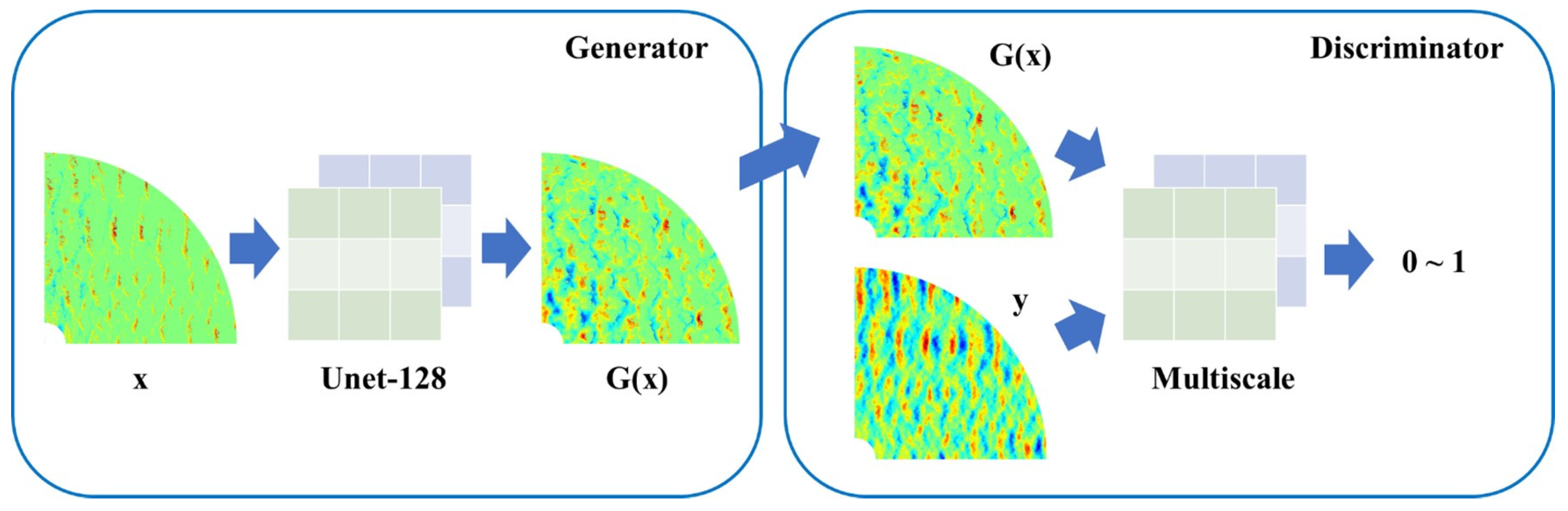
3.1. Simulated Wave Surface Retrieval

The model proposed in this study is compared against the traditional Pix2Pix model and the CNNSA model. The Pix2Pix model serves as the baseline, representing the original, unenhanced version, while the CNNSA model, introduced by Zuo et al. [23], provides an additional benchmark for evaluation.

An error analysis formula, derived from Section 2.3, is applied to compute error statistics using the test set data, which is categorized by sea state. The retrieval errors for each model are summarized in

Table 5. Statistical analysis of retrieval result errors for various models.

Sea State	Metrics	Atten-Pix2pix	Pix2pix	CNNSA
Level 3	MSE	34.215	38.861	41.325
	PSNR	35.155	32.236	31.868
	SSIM	0.9021	0.8738	0.8544
Level 4	MSE	40.214	42.657	45.364
	PSNR	32.215	32.021	31.235
	SSIM	0.8644	0.8242	0.7963
Level 5	MSE	46.025	49.754	53.215
	PSNR	31.897	31.235	30.440
	SSIM	0.8126	0.7754	0.7151
Level 6	MSE	51.332	58.484	67.558
	PSNR	31.026	30.460	29.792
	SSIM	0.7566	0.6563	0.6024

.

Based on the data presented in Table 5, it is evident that under four different sea state conditions, the proposed Atten-Pix2Pix model achieves the lowest MSE values and the highest PSNR values. Additionally, the SSIM metric approaches its ideal value of 1, underscoring the model’s exceptional performance across these evaluation metrics. In contrast, the CNNSA model demonstrates inferior performance compared to both competing models in all three metrics, highlighting its limitations for retrieval tasks. These shortcomings are particularly pronounced under level 6 sea state conditions.

For further analysis, the two vertical components, $k_x$ and $k_y$, of the wave number vector are derived using the Quadratic Fourier Transform of both the original wave surface and the wave surface reconstructed by the proposed model. To facilitate a comprehensive comparison of wave number spectra across sea states three to six, wave number spectrum images are generated by normalizing the two vertical components with respect to the input spectral peak wave number, $k_0$, as illustrated in Figure 11.

Additionally, a pixel-wise difference analysis is conducted between the reconstructed and original images, focusing on the relative height discrepancies between the predicted values and the actual measurements. The results are obtained by first simulating an idealized 3D wave surface using the methodology described in Section 2.1.1. Subsequently, modulated radar images are simulated using the principles in Section 2.1.2 to represent X-band marine radar images. These modulated radar images are then used as input to the Atten-Pix2Pix model, which performs retrieval to reconstruct the 3D wave surface. Finally, the reconstructed wave surface is compared against the idealized 3D wave surface using quantitative metrics to evaluate the model’s performance and accuracy. The results of this pixel-wise difference analysis are depicted in Figure 12.

In the wave number spectrum of level 3 sea states (Figure 11a), the overall fitting performance of the reconstructed wave surface meets expectations, demonstrating a high level of accuracy. Notably, the fitting accuracy within the wave number concentration region is exceptionally high. Additionally, the fitting results in the scattered wave number regions are generally satisfactory, though occasional data gaps are observed.

Under level 3 sea state conditions (Figure 12a), the relative height difference between the predicted wave surface and the original wave surface remains within a range of ±0.2 m. Near the radar center, this relative height difference approaches zero, while in regions farther from the radar center, both the frequency and magnitude of relative differences are minimal. A comprehensive analysis of elevation differences across all sea states indicates that the relative errors are smallest in sea state level 3, leading to enhanced prediction accuracy under these conditions.

In the wave number spectrum of the level 4 sea state (Figure 11b), the generated data exhibit a high degree of correlation with the original dataset, particularly in regions with concentrated wave number energy. However, in areas with lower wave numbers and sparse energy, the fitting performance is less accurate, leading to some missing data points. Despite this limitation, the overall representation of the wave surface remains largely unaffected, and the fitting results are deemed satisfactory.

As shown in Figure 12b, the relative height difference between the generated wave surface and the original wave surface is maintained within a range of ±0.3 m. Near the radar center, this difference is predominantly positive, while a mix of positive and negative differences is observed in regions farther from the radar center, resulting in slightly increased variation overall.

In the wave number spectrum of the level 5 sea state (Figure 11c), the overall fitting performance of the wave surface meets expectations and demonstrates commendable accuracy. This is particularly evident in the concentrated wave number region, where the fitting results are highly effective.

At sea state level 5 (Figure 12c), the relative error between the generated wave surface and the original wave surface is predominantly observed in regions farther from the radar center, with some pixel points exhibiting an error range within ±0.7 m. This phenomenon can be attributed to the increased complexity of the sea state conditions and the inherent randomness in data selection, both of which contribute to the observed variations.

In the wave number spectrum of the level 6 sea state (Figure 11d), the overall predictive fitting of the wave surface demonstrates a relatively high degree of accuracy. In regions where wave number energy is concentrated, the generated image closely aligns with the original image, achieving a highly accurate fitting effect. Conversely, in areas with scattered wave numbers, the fitting performance is less satisfactory, with some discrepancies observed. However, these discrepancies are minimal compared to those in concentrated regions, resulting in an overall commendable fitting performance.

At sea state level 6 (Figure 12d), the total wave height exhibits significant variation over a relatively wide range. Within the radar scan area, error distributions are observed, with the error range constrained to ±1.0 m. This variation can be attributed to two primary factors. First, the generation of linear waves involves inherent randomness, leading to individual data points that may not fully represent the overall characteristics of the dataset. Second, the higher effective wave height and increased complexity typical of level 6 sea states contribute to the observed discrepancies.

A longitudinal comparison of the wave number spectrum across different sea states reveals that the accuracy of the fit between the generated images and the original images progressively decreases with increasing sea state severity. This trend is observed in both regions of concentrated and sparse energy. Nonetheless, within each individual sea state, the model demonstrates commendable predictive capability, maintaining errors within an acceptable range.

Similarly, a longitudinal analysis of wave surface differences indicates that as the sea state intensifies, the discrepancies between the generated and original wave surfaces also increase. In other words, the fitting performance of the generated images deteriorates relative to the original images, consistent with the observations from the wave number spectrum analysis.

This phenomenon can be attributed to the increasing complexity associated with higher sea states. As sea conditions become more severe, nonlinear interactions and breaking waves exert a significant influence on the prediction results. Consequently, both the retrieval accuracy of the model and the fidelity of the measured wave surfaces are adversely affected.

3.2. Measured Wave Surface Retrieval

In this section, we conduct a 3D wave surface retrieval analysis using the proposed retrieval model described in Section 2.2, applied to measured sea clutter data. The data are sourced from sea clutter files (*.POL) collected by the WAMOS II radar system (OceanWaveS GmbH, Lüneburg, Germiny). These files are accessible via the WinWaMoS software (version 3.03) platform through its menu-based interface.

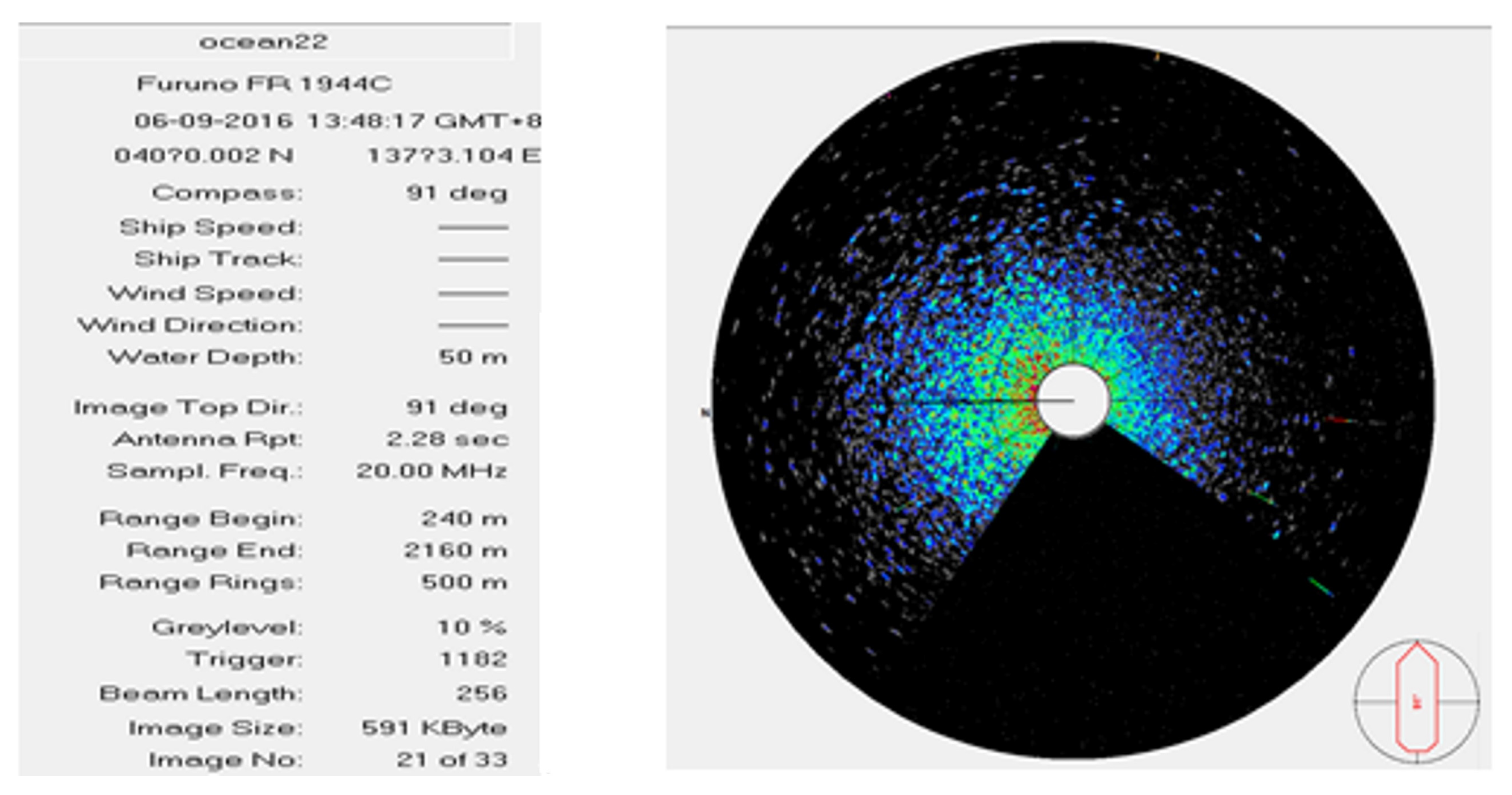
As shown in Figure 13, the sample data are collected on 9 June 2016 at 13:48:17 local time. The geographical coordinates of the data collection site are latitude 40°02′ S and longitude 137°03′104″ E. The recorded compass angle is 91°, with a bow angle of 1°. The water depth at the location is approximately 50 m.

The acquisition system is configured with an antenna rotation period of 2.28 s, a signal transmission frequency of 20 MHz, and a polar radius acquisition range spanning approximately 240 to 2160 m. Additionally, the signal image resolution is set to 256 pixels, with a tolerance of ±10%. Within each acquisition cycle, 33 groups of data are sampled over a range of $0$ to $3/2\pi$.

The collected Polar Data (POL) file consists of two primary components: the header and the image. The header includes essential WaMos configuration parameters, while the image is stored as a binary-encoded file.

Since the image data are stored in a range-to-azimuth format, it is necessary to construct a 3D array for effective interpretation. The first dimension corresponds to the data volume within a single cycle, while the third dimension represents the distance associated with each image. The second dimension is computed to accurately represent the azimuthal extent of the images.

Following the analysis of the POL file, a coherent color scheme is applied to generate both the original WAMOS II image and its corresponding MATLAB reproduction using the same POL file, as illustrated in Figure 14.

After processing and saving the sea clutter data in MATLAB, an angular range from 0 to $\pi /2$, centered on the ship’s heading, is selected. This selection enables the generation of a sequence diagram illustrating the sea clutter distribution relative to the ship’s heading, as depicted in Figure 15.

To validate the proposed method, the approach from Reference [28] is used as a benchmark to compare the retrieval accuracy of the three methods, as real-world tools for capturing full wave surfaces are currently unavailable. This benchmark predicts temporal and spatial wave evolution by calculating eigenvalues of the nonlinear Schrödinger (NLS) equation from measured wave height data using the inverse scattering transform of the third-order NLS equation.

First, a fixed point $[1000, 1000]$ is selected from the reconstructed three-dimensional wave surface as the monitoring point. A 100 s wave height time-history dataset is extracted from this point, and its upper and lower envelopes are identified.

The initial data and corresponding envelopes are then input into the NLS equation, where the model computes the eigenvalues of the equation. Using these eigenvalues, the model predicts the subsequent 400 s of wave height envelopes.

The 400 s wave height sequences at the monitoring point are predicted using the proposed model, the traditional Pix2Pix model, and the CNNSA model. These predictions are compared with the benchmark wave height envelopes, as shown in Figure 16. The Mean Square Error (MSE) between the predictions of each model and the benchmark is computed and summarized in

Table 6. Error of retrieval results for different models.

Model	MSE
Atten-Pix2pix	0.3215
Pix2pix	0.4437
CNNSA	0.5021

.

The analysis results indicate that the model proposed in this study demonstrates superior performance. As shown in Figure 16, the wave height predictions generated by the Atten-Pix2Pix model exhibit the highest degree of consistency with the envelope results derived from the NLS equation. Compared to the retrieval results obtained using the Schrödinger equation model, the proposed model achieves a Mean Square Error (MSE) of 0.3215, which is notably lower than that of the other two models. This result highlights the effectiveness and superiority of the proposed method in this study.

4. Conclusions

This study addresses the challenges of sea state observation and emergency requirements for ship navigation by proposing a wave retrieval methodology utilizing both simulated data and ship-borne WAMOS II radar system data. First, linear wave theory is employed to simulate realistic wave surfaces and generate paired modulated radar sea clutter data. Based on these numerical simulation data, a predictive model dataset is constructed, and an attention-based Pix2Pix model is applied to facilitate the retrieval of radar sea clutter data into sea wave surfaces. Finally, the proposed method is validated using measured radar image data, with the retrieved sea wave surfaces compared against those derived from the Schrödinger equation. The results demonstrate that the proposed method effectively establishes a mapping relationship between paired data sets and achieves strong consistency with predictions, enabling accurate retrieval from radar waves to 3D wave surfaces. This highlights the potential of the method for practical applications in wave retrieval and navigation safety.

Building on the findings of this study, future research could expand upon the analysis presented here, which forms the foundation for further developments aimed at improving the proposed method’s robustness and applicability. Specifically, the following directions are suggested for future work:

• Future research could include spatial radar signal attenuation in numerical simulations, considering both radar image attenuation along the wavefront and the effects of attenuation over long distances. This would significantly improve the accuracy of wave surface reconstruction under realistic ocean conditions. Such an analysis is crucial as radar signal attenuation can lead to errors in wave height retrieval, especially when the radar beam is parallel to the wavefront or when the observation distance is large.
• Further validation of the proposed method is needed beyond the JONSWAP spectrum, including tests with realistic wave spectra derived from experimental data. This would allow for a more comprehensive assessment of the method’s generalization and performance across various ocean environments, providing a better understanding of its limitations and potential improvements.
• An array of buoys on the sea surface could be deployed to measure three-dimensional wave surfaces, serving as a benchmark to validate the accuracy of the retrieval model. Using real-world buoy data to cross-validate the simulation results would provide essential insights into the method’s practical applicability.

These proposed future developments will not only validate the results obtained in this study but also address the influence of various environmental factors on wave surface retrieval, ensuring that the method performs well under realistic conditions.