Convenient Method for Large-Deformation Finite-Element Simulation of Submarine Landslides Considering Shear Softening and Rate Correlation Effects

Abstract

Submarine landslides pose a serious threat to the safety of underwater engineering facilities. To evaluate the safety of undersea structures, it is important to estimate and analyze the sliding processes of potential submarine landslides. In this study, a convenient model for simulating submarine landslide processes is established by using Abaqus Eulerian large deformation technology with an explicit finite element framework. The VUSDFLD Fortran subroutine is used to consider the strain-softening and rate-dependency characteristics of soil shear strength. The proposed method is validated by comparing its results with experimental data and those of mainstream numerical methods. Then, the results of a dynamic analysis of typical potential submarine landslides in the Shenhu sea area are analyzed using the proposed method. Case studies are carried out under different soil shear strength distributions, and the influence of initial stress is also analyzed. The shear strain-softening and rate-dependency effects are highly involved in the runout process. The simulated landslide’s failure mode is consistent with the geophysical interpretation of existing landslide characteristics.

1. Introduction

Submarine landslides are common in continental margins and island slope areas, and the large number of landslide mass movements, involving the movement of sand, clay, and gravel, can cause great damage to submarine pipelines, cables, and other underwater facilities [1,2,3,4,5]. Large submarine landslides even pose a risk of triggering catastrophic tsunamis [6,7]. How to reasonably simulate and predict the movement processes of submarine landslides has thus become a key aspect of assessing the risk of the impacts of submarine landslides [8], as well as in the study of the transport and sedimentation system of continental slope areas.

The study of the sliding process of submarine landslides includes multiple disciplines, such as geotechnical mechanics and fluid mechanics (as shown in Figure 1), making it difficult to simulate the entire process using a unified model [9].

As matters stand, the main methods for simulating the mass movement of submarine landslides are as follows: analytical methods based on rigid bodies [10,11], single-phase plastic fluid methods [12,13], multiphase flow methods [14,15,16,17], large deformation finite element methods [18], material point methods [19,20], discrete element methods/smoothed particle hydrodynamics [21,22], and CFD-DEM coupling methods [23,24].

Analytical methods based on rigid body assumption can achieve high efficiencies at low computational costs since they do not require complicated theoretical derivation. However, the sliding soils of most landslides actually undergo large deformation. Therefore, using a rigid body assumption would cause a certain degree of difference in the results.

Imran et al. [12] developed a numerical program (BING) to simulate the runout of submarine landslides, which incorporated the Bingham, Herschel–Bulkley, and bilinear rheologies of viscoplastic fluids. Using the depth-averaged method, the two-dimensional runout is essentially simplified as a one-dimensional problem. On this basis, the Bing program has been further expanded to include the whole submarine landslide process, consisting of four phases: the initial flow stage, the water wedge development stage, the hydroplaning stage, and the post-hydroplaning stage [13]. However, several artificially assumed parameters, which need to be subjectively assigned, were introduced to distinguish different stages. It is not clear if the program can be used for complex morphologies, as the sliding material might not be divided into the shear and plug layers [25].

Multiphase flow methods can handle interactions between sliding soil and the environmental water to a certain extent [14,15,16,17]. However, they cannot reasonably reflect the complex stress–strain relationship of the landslide mass, especially in the early phase of sliding. In the early and middle stages, the landslide mass is more aligned with the scope of soil mechanics. Multiphase flow methods cannot accurately describe the shear softening process of sliding soil. Discrete element methods (DEMs) and smoothed particle hydrodynamics (SPHs) can deal with mesh distortion problems well since they are mesh-free techniques. However, difficulties still exist in the determination of boundary conditions when they are applied to the simulation of actual landslide problems, and the artificial stress technology can lead to high stress [21,22]. Furthermore, CFD-DEM coupling methods have also been used for the runout simulation of submarine landslides [23,24], showing good prospects. However, their computational cost is high when particle size increases, especially in the case of real-scale submarine landslide simulations.

The shear strength of sliding soil plays an important role in the runout of submarine landslides. Cohesive marine soils, especially those with medium to high sensitivity, exhibit not only shear strength softening characteristics under shear loads but also rate-dependency effects during the mass movement of the submarine landslide [26,27,28]. The aforementioned studies did not take these complex shear characteristics into account quantitatively. The large deformation finite element method (RITSS) [18,29] and material point method (MPM) [19,20] are two prominent methods used in large deformation analysis. The RITSS approach is based on the “remeshing and interpolation technique with small strain.” It was initially proposed by Hu and Randolph [30] and was then extended to an Abaqus-based dynamic RITSS approach by Wang et al. [18]. In the dynamic RITSS approach, a small strain incremental analysis step is executed first; then, the configuration is updated by the new boundary node positions. After that, the new configuration is re-meshed, and all the variables, such as velocities, accelerations, stresses, and material properties, are mapped to the new mesh. The MPM originates from the particle-in-cell method in computational fluid dynamics [31]. The continua are discretized by Lagrangian particles moving over a fixed Eulerian background grid. The materials’ mechanical and kinematic properties (mass, volume, density, velocities, momentum, deformation gradients, and stresses) are recorded and updated within the particles, and the Eulerian mesh is only used for calculation at each incremental step. Both of these methods have been adopted and validated in runout simulations of submarine landslides in which the shear strain-softening and rate-dependency effects were also incorporated [18,19,20,29]. However, in these two methods, some key but unpublished in-house programs regarding remeshing, interpolation, and numerical algorithms are needed. This gap poses high theoretical and technical requirements for the engineering community.

This article proposes a convenient simulation method for the runout simulation of submarine landslides based on the Eulerian analysis technology of Abaqus/Explicit. The used Eulerian analysis technology provides a large deformation calculation method in an explicit finite element scheme [32]. In each incremental step of the Eulerian analysis, a Lagrangian calculation is first performed, and then the new variables are mapped to the fixed Eulerian background mesh to achieve material flow [33,34,35]. This technology is effective for applications involving extreme deformation, up to and including fluid flow. The VUSDFLD Fortran subroutine provided in Abaqus can be applied to conveniently take into account the complex stress–strain relationships. So, the dynamic runout process of submarine landslides involving the shear strain-softening and rate-dependency characteristics of sliding soil can be implemented with VUSDFLD. The proposed convenient method can facilitate the common engineers to quickly analyze the runout process of submarine landslides.

2. Materials and Methods

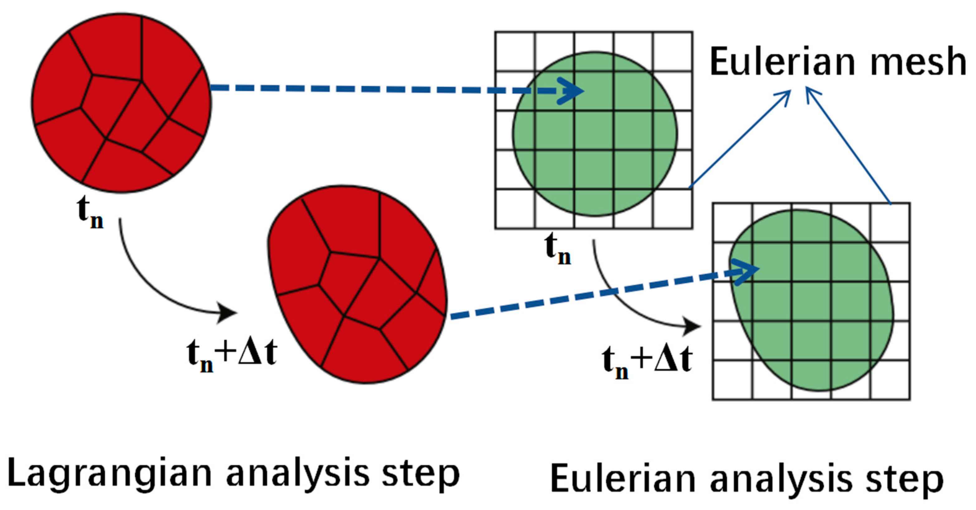
2.1. Eulerian Analysis Technique

The Eulerian large deformation analysis technique implemented in Abaqus/Explicit uses an explicit time integration scheme [32]. In each time increment, the Eulerian analysis is internally divided into two steps, a Lagrangian analysis step and an Eulerian analysis step; the steps are shown in Figure 2.

At the beginning of each time increment, Δt, a traditional Lagrangian analysis step is first performed, in which the movement of the continuum is treated as a function of the material coordinates and time. The nodes of the Lagrangian mesh move together with the material, and elements deform as the material deforms (see Figure 2, left side). At the end of the Lagrangian step, a tolerance is adopted to determine which elements are significantly deformed. Elements with little or no deformation will remain inactive during the Eulerian step to improve computational performance. In the Eulerian analysis step, an Eulerian reference mesh (see Figure 2 right side), which remains undistorted is used to trace the motion of the material in the Eulerian domain. Deformation is suspended during the Eulerian analysis step. The elements with significant deformation are automatically remeshed, and the corresponding material flow between neighboring elements is then computed.

The central difference rule is adopted for the solution of the non-linear differential equations. The unknown solution for the time $t+\Delta t$ can be calculated directly according to the solution at time t without iteration. Explicit calculations are not stringently stable, but their numerical stability can be guaranteed via the introduction of the critical time step size $\Delta t_{\mathrm{crit}}$. For Eulerian analysis, the stable time increment size is adjusted automatically to prevent material from flowing across more than one element in each increment. $\Delta t_{\mathrm{crit}}$ is calculated in each time step and can be described using the characteristic element length L_e and the dilatory wave speed c_d:

$$\Delta t_{\mathrm{crit}}=L_e/c_{\mathrm{d}}$$

(1)

Compared with the traditional Lagrangian method, the Eulerian analysis technique is more suitable for large deformation calculations. For the runout simulation of a submarine landslide, cohesive soils with medium to high sensitivity exhibit significant strength-softening characteristics under shear loads [26,27,28]. The strain-softening and rate-related effects of landslide soil should be taken into account quantitatively in the soil’s constitutive model. However, this feature is not directly provided in the Abaqus/Explicit module. Thus, this paper proposed a convenient method (more on that later) to achieve this function by using the VUSDFLD Fortran subroutine interface.

2.2. Detail Methodology

A long preset rectangular computational domain consisting of a soil domain and a void domain is first chosen to ensure that the submarine landslide mass cannot flow out of the boundary. The entire computational domain was set as the Eulerian part, and the first-order reduced integration hexahedral Eulerian element, EC3D8R, was used for calculation. The total stress method is adopted since EC3D8R does not involve pore pressure, and, therefore, the buoyant unit weight, ${\gamma }^{\prime }$, is used for the landslide soil. Velocity-constrained conditions are applied on the boundary of the Eulerian domain.

The Tresca soil model, which simulates linearly elasto-plastic behavior, was adopted to describe the mechanical properties of a submarine landslide mass. It can be defined by three parameters: undrained shear strength, S_u; elastic modulus, E; and Poisson’s ratio, υ. The undrained shear strength is governed by shear strain rate and soil remolding. The peak strength increases with the shearing rate but decreases with the absolute plastic shear strain. Then, the Tresca model can be considered through an enhanced Herschel–Bulkley (H-B) model [18,19,20,26,27,28]. During the runout process of a submarine landslide, the soil’s strength is gradually reduced as the absolute plastic shear strain accumulates. This process continues until a fully remolded condition is achieved. At the same time, the current undrained strength changes with the dynamic shear rate. The current undrained strength, S_u, at the Gauss points can be expressed in terms of shear strain rate, $\dot{\gamma }$, and accumulated absolute plastic shear strain, ξ:

$$s_u=s_{u0}\alpha \beta =s_{u0}\left[{\delta }_{rem}+\left(1-{\delta }_{rem}\right)e^{-3\xi /{\xi }_{95}}\right]\left\{1+\eta {\left(\frac{\dot{\gamma }}{{\dot{\gamma }}_{ref}}\right)}^n\right\}$$

(2)

where ${\delta }_{rem}$ is the inverse of the soil sensitivity, S_t, denoting the ratio between the fully remolded and initial shear strengths; ${\xi }_{95}$ is the accumulated shear strain when a 95% soil strength degradation occurs between the intact and fully remolded conditions; $\eta$ is the viscosity coefficient and n is the shear-thinning index; ${\dot{\gamma }}_{ref}$ is the reference shear strain rate; and $\alpha$, $\beta$ are the coefficients of the strain softening and the strain rate dependency, respectively.

The shear strain-softening and rate-dependency model (Equation (2)) was incorporated into ABAQUS based on the Tresca soil constitutive model using the user subroutine VUSDFLD. Because the field variables of Eulerian element EC3D8R cannot be called directly in VUSDFLD, the temperature, as a dummy variable, is called in the VUSDFLD subroutine as an initial state variable to allow a variation in temperature that is identical to the initial undrained shear strength, S_u0. This approach has been used in the study of the penetration resistance of bucket foundations and has proven to be effective [35]. In the computational domain, an initial temperature field that is identical to S_u0 is provided by an “*initial conditions” keyword, while in the void domain, the temperature is zero. The accumulated absolute plastic shear strain, ξ, in Equation (2) is given by the sum of the accumulated absolute plastic shear strain, Δε_p1 − Δε_p3. Δε_p1 and Δε_p3 are the cumulative major and minor plastic shear strains, respectively, in each increment (dt). The shear strain rate, $\dot{\gamma }$, in Equation (1) can be computed using Equation (3):

$$\dot{\gamma }=\frac{\left(\Delta {\epsilon }_1-\Delta {\epsilon }_3\right)}{\Delta t}$$

(3)

where $\Delta {\epsilon }_1$ and $\Delta {\epsilon }_3$ are the cumulative major and minor principal strains over the duration of $\Delta t$. All involved strain components and temperature dummy variables can be obtained using the utility routine VGETVRM. The variations in ξ and $\dot{\gamma }$ can be captured through simple algebraic operations with the help of state variables.

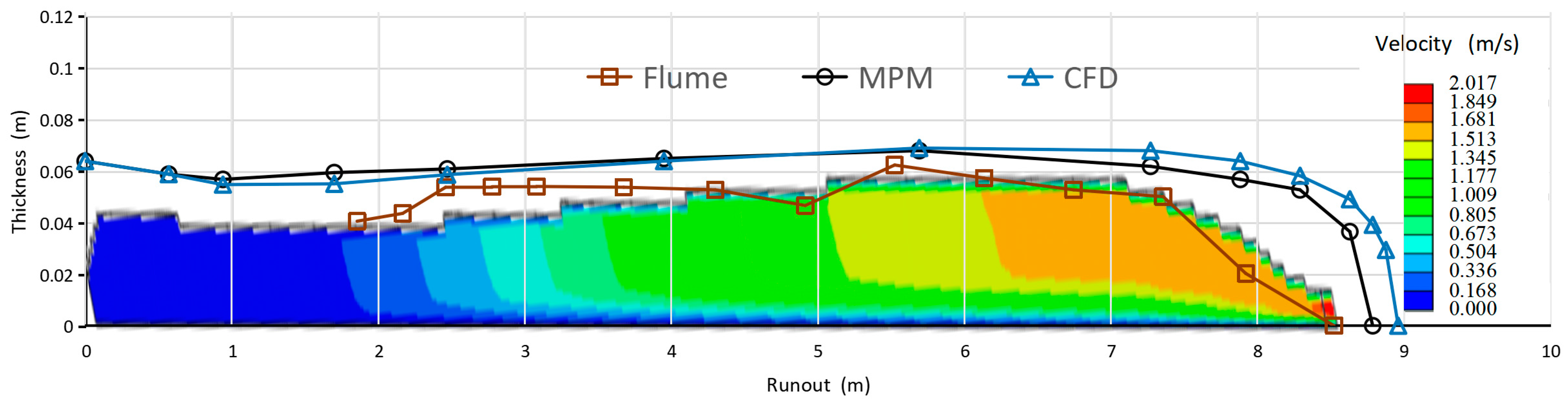
2.3. Approach Validation

A flume experiment (Case 1) and a numerical model (Case 2) are chosen for the validation of the proposed approach.

A laboratory study of slurry runout induced by a dam break was carried out by Wright and Krone [36] by instantaneously releasing a bentonite slurry from an upstream reservoir into a rectangular flume with a constant slope of 3.44°. The initial length of the slurry was 1.8 m; the initial height was 0.3 m; the yield strength s_u0 was 42.5 Pa; Young’s modulus was taken as 100s_u0; the slurry density was 1073 kg/m³; and the reference strain rate was 193.2 s^–1, which can be expressed by the yield strength divided by the dynamic viscosity. The base of the flume was assumed to be a no-slip boundary. The model parameters for Equation (2) in Case 1 are shown in

Table 1. Model parameters of simulation cases.

Case	θ/(°)	Su0/kPa	η	n	${\dot{\mathit{\gamma }}}_{\mathit{r}\mathit{e}\mathit{f}}$	St	${\mathit{\xi }}_{95}$	τ/kPa	V0/m.s−1	${\mathit{\gamma }}^{\prime }$/kN.m−3
1	3.44	0.0425	1	1	193.2	1	-	0.0425	0	10.73
2	2	5	0	-	-	5	10	1.0	1.0	6.0

. The element sizes of 0.005 m, 0.004 m, and 0.0025 m show almost the same results, so the element size 0.005 m with the time step t = 3.3 × 10⁻⁴ s can satisfy the computing requirement.

Figure 3 shows that the runout results predicted by the proposed approach agreed reasonably well with the experimental observation and the numerical results of MPM and CFD [18]. The divergence is 3.3% compared with the experimental data and 8.6% compared with the CFD results.

A simple designed submarine landslide case, which has also been used in other studies [18,19,20], is adopted here for model validation (Case 2). The simulation results are then compared with those of the RITSS method [18]. The geometry of the submarine landslide (showed in Figure 4) is trapezoidal and is preset on a slope with an inclination angle θ = 30°. The height and base width of the trapezoidal landslide are 5 m and 48.66 m, respectively. The seabed is modeled as a rigid body. The contact between the seabed and sliding soil is implemented as “general contact,” with a frictional strength, τ, on the seabed–sliding mass interface. Young’s modulus was taken as 500s_u0. The soil strength parameters of the landslides used in the validation model are shown in Table 1. The element sizes of 0.25 m, 0.2 m, and 0.15 m show almost the same results, so the 0.25 m element size with the time step t = 3.86 × 10⁻⁴ s can satisfy the computing requirements. The comparison of the results of the two case studies is shown in Figure 5. The simulated runout basically presents a similar trend to the RITSS method, with a maximum divergence of 10.7% at the final runout distance. Figure 6 shows the softened effect of soil due to the shear disturbance during the sliding process. The softening ratio distribution is also consistent with that of the RITSS method. The inclusion of soil softening causes wedges to form at a 45-degree inclination, with the shearing becoming concentrated within the weakened soil between the wedges. Both Case 1 and Case 2 indicate that the proposed method can provide reasonable simulation results.

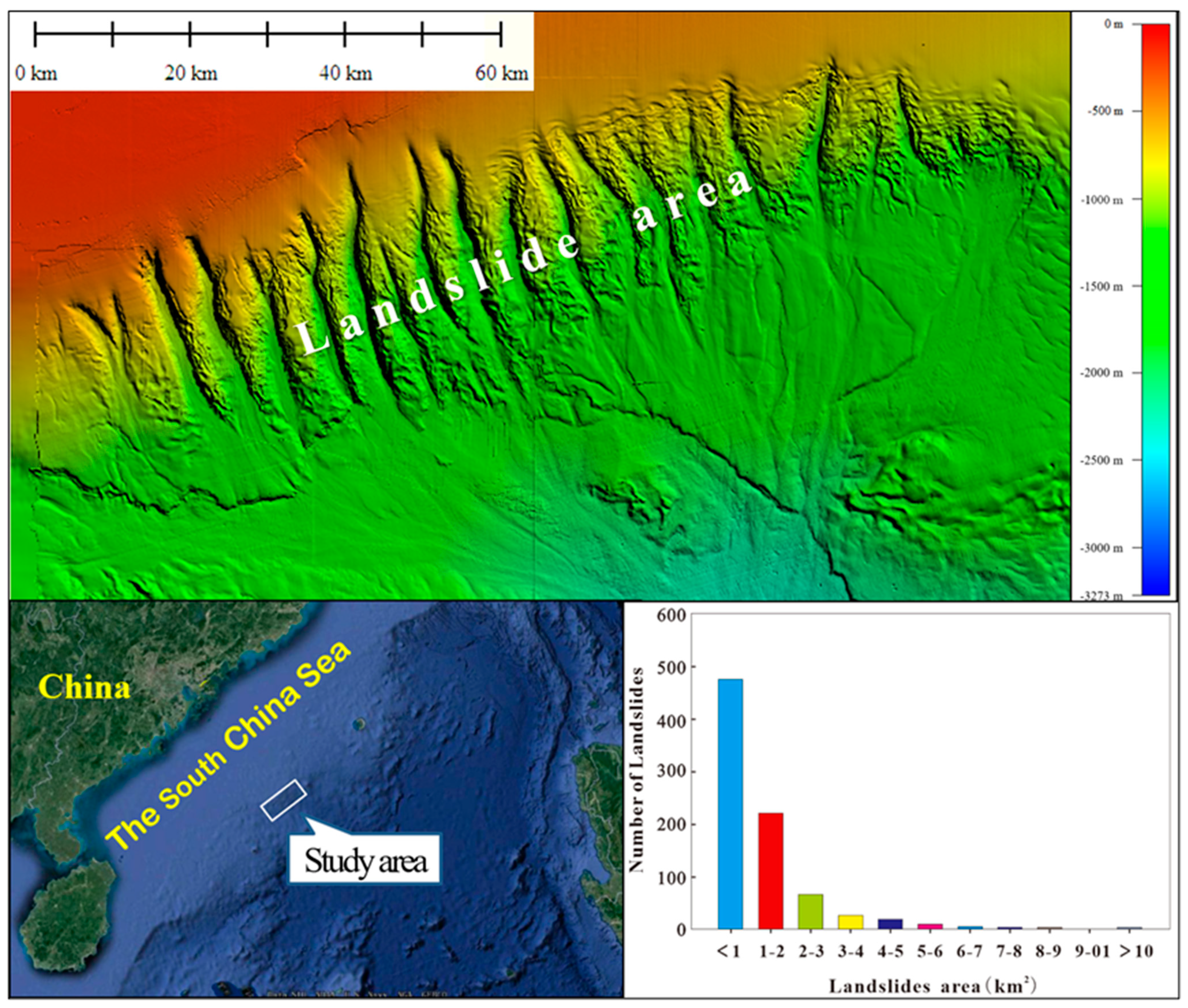
3. Numerical Modeling of Submarine Landslide in Shenhu Sea Area

3.1. Engineering Geological Conditions

The Shenhu sea area, which is on the northern slope of the South China Sea, is not only rich in oil and gas resources [37] but also prone to submarine landslides [38,39,40]. A great number of small submarine landslides have been identified in this area [41,42]. The great potential for submarine landslides would pose a great threat to the safety of undersea pipelines across this area, as shown in Figure 7. Multibeam topography has shown that the heights of the landslide scarps, which are mainly located at the sidewall and the interfluve of the canyon, are basically between 8 and 125 m, and the maximum local slope can reach 26.6° [43]. The soil in the Shenhu sea area has medium or high soil sensitivity based on the drilling test and the in situ CPT test [44,45], and the undrained shear strength exhibits linear and segmented linear growth with increasing burial depth. The intact undrained shear strength of the soil, S_u0, can be expressed as

S_u0 = S_um + kz

(4)

where S_um is the shear strength at the mudline, k is the shear strength gradient, and z is the burial depth.

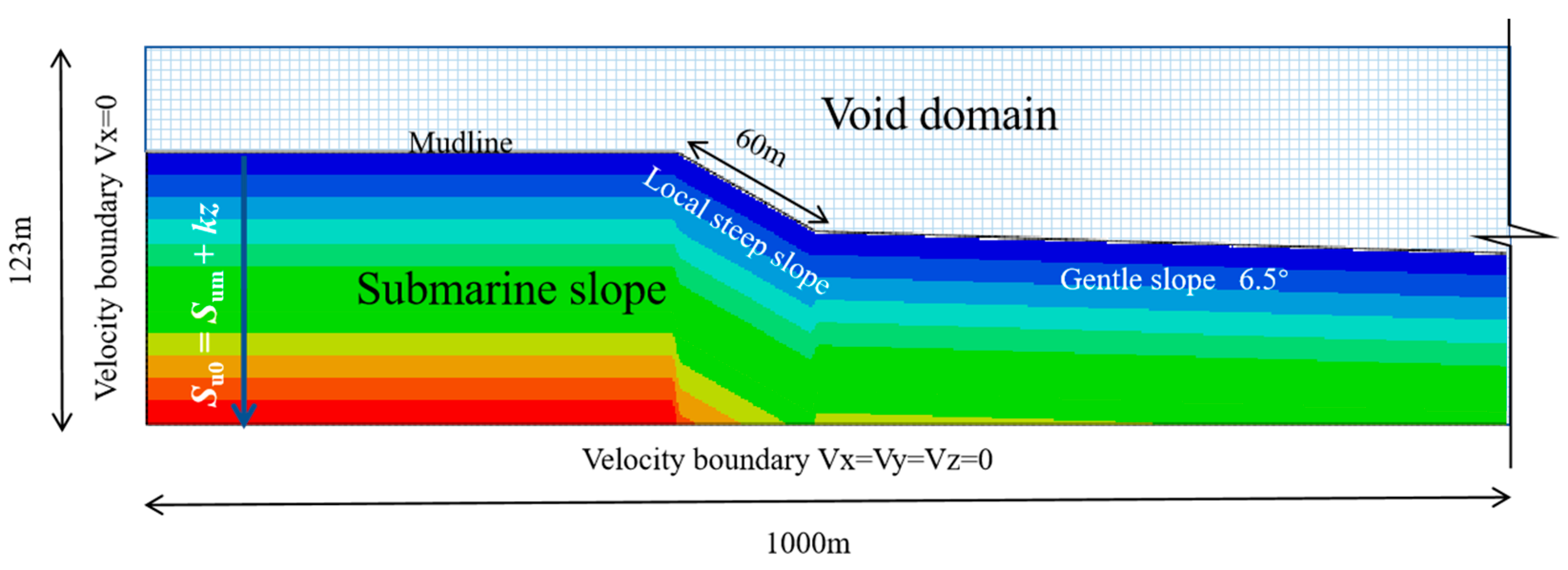
3.2. Numerical Modeling of Typical Submarine Landslides

According to the geological engineering background of the Shenhu sea area, a typical submarine landslide model is chosen for runout analysis. The terrain includes horizontal sections, local steep slope sections, and gentle slope sections. A 6.5° gentle slope is used to simulate the regional terrain slope. Local steep slopes are generally located at the landslide scarp. Here, a 30° slope to the horizontal (23.5° compared to the 6.5° seabed), which is close to the maximum local slope of 26.6°, is used to simulate a slope erosion trigger mechanism. The initial submarine slope adopted here is actually in an unstable state (i.e., it has a slope stability coefficient less than 1.0), since otherwise, a submarine landslide will not occur. Thus, the stability analysis of the submarine slope has not been performed here. A schematic diagram of the submarine landslide model is presented in Figure 8.

The Eulerian element size is 1 m × 1 m × 1 m, with the time step t = 4.0 × 10⁻⁴ s. The intact undrained strength at the mudline is S_um = 2~5 kPa; the shear strength gradient is k = 1.15~1.25 kPa/m; the soil sensitivity, S_t, is chosen as 2.0, 3.0, 4.0, and 5.0, corresponding to medium sensitivity to extra-high sensitivity, respectively; the elastic modulus is E = 500 S_u; and Poisson’s ratio is υ = 0.49. The shear-softening and rate-dependency parameters are η = 0.3, n = 0.5, and ${\xi }_{95}$ = 10.0. A soil density ρ_s = 600 kg/m³ (ρ_s = Saturation density – water density) is used in the model, so the weight of the soil is actually the submerged weight. In this study, we conducted runout simulations of various cases based on the typical submarine landslide model. The following section presents a detailed analysis and discussion of the results obtained.

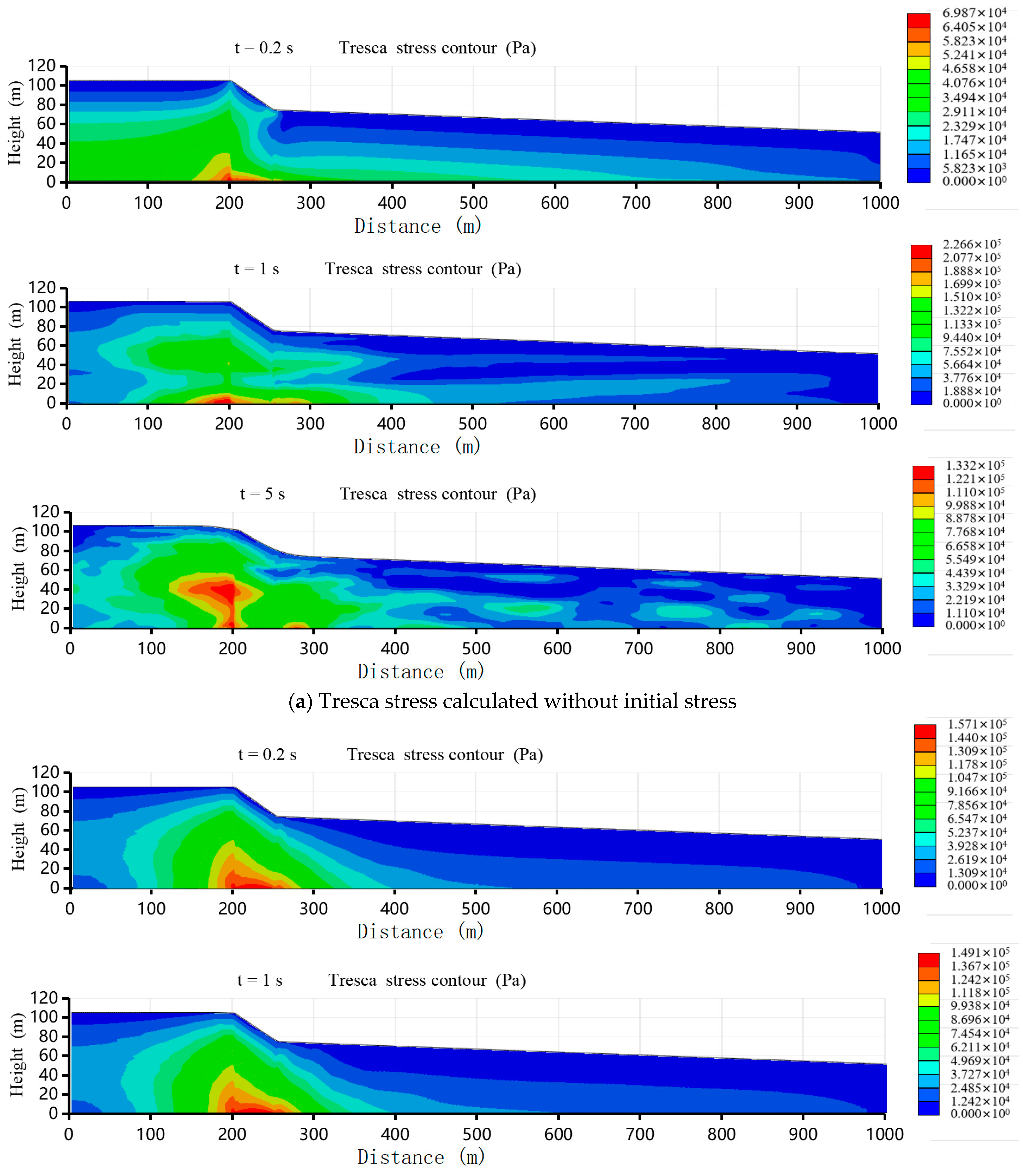
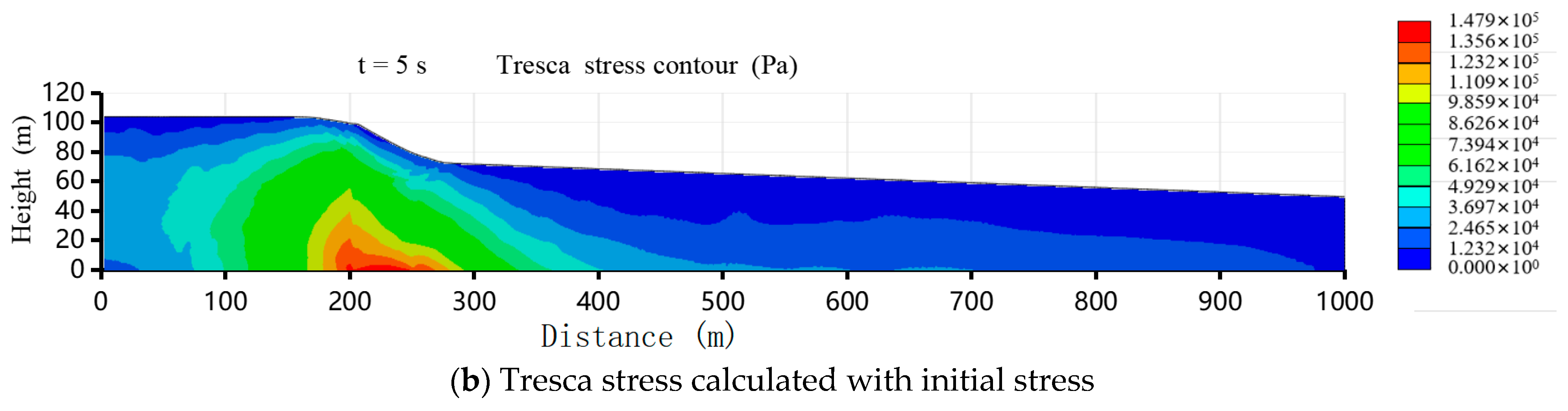
4. Results and Discussion

The initial in situ stress distribution in the seabed may have an impact on a landslide’s mass movement process. In this paper, the in situ stress field under self-weight is taken as the initial stress. In order to illustrate this, two cases with and without in situ stress are first calculated. Figure 9 and Figure 10 show the Tresca stress and velocity distributions at different time points, respectively, in the case of S_um = 5 kPa, K = 1.15 kPa/m, and S_t = 4.0. It can be seen that both cases show a shallow landslide failure mode, which is consistent with the stability analysis of the submarine slope and the geophysical interpretation of existing landslide characteristics [16,40,41,42,45]. In the case that the initial stress has not been taken into account, the self-weight load can lead to large fluctuations in the stress field. The additional stress fluctuation in turn has a negative effect on the accuracy of the velocity field. As shown in Figure 10, the velocity of the landslide in the early stage (for example, t = 1 s) is higher than when initial stress is considered. This is because the gravitational load poses an overall dynamic vertical additional velocity at early stages. However, the velocity decreases quickly over time due to the subsequent stress oscillations, eventually leading to a rather smaller landslide runout distance. Therefore, in the subsequent calculations, an initial stress field is adopted to balance the influence of the gravitational load.

Figure 11 shows the equivalent plastic strain during the landslide process for the cases both with and without the strain-softening and rate-dependency effects. It can be seen that when the strain-softening and rate-dependency effects are incorporated, a distinct difference can be seen in the submarine landslide runout process, although both cases have almost the same initial landslide sliding surface depth (about 25 m). The shear zone presents similar features in the early stage (for example, t = 1 s). As time goes on, the strain-softening and rate-dependency effects gradually come into play, corresponding to the accumulation of absolute plastic shear strain and the shear strain rate. The sliding soil without the strain-softening and rate-dependency effects decelerates quickly after sliding down the local steep slope, and a much thicker deposit can be found. In contrast, the sliding soil with the strain-softening and rate-dependency effects shows much better ductility, which means a much larger runout distance. The distance from the slope toe to the front of the final mass transport deposition is 48 m and 166 m, respectively, for the two cases.

The accumulated absolute plastic shear strain induces a continuous downward trend in the soil’s shear strength (strain-softening), while the shear strain rate has a positive correlation with the shear strength. The shear strength of the sliding soil and the strain shear rate effect are shown in Figure 12 and Figure 13, respectively. It can be seen that S_u in the shear zone changes gradually with the shear remolding and shear strain rate-dependency. At the early stage of the landslide process, the soil accelerates at a high velocity when sliding down the local steep slope. At the same time, the accumulated absolute plastic shear strain of the soil is not large enough, and, therefore, a local high shear strength occurs in the shear zone due to the combination of a higher rate-dependency effect and a lower strain-softening effect. This also leads to a relatively small sliding velocity when the shear layer has not been significantly remolded. At the middle to late stages of the sliding process, the strain-softening effect caused by the shear disturbance gradually increases.

The shear strength distribution of the soil and the slope angle are the main controlling factors of the mass movement of a submarine landslide. The effect of the shear strength distribution on the landslide process is analyzed by comparison of different combinations of S_um and k, which is described by Equation (3), when the initial geometric configuration is the same. This is an approximate equivalence of submarine areas that have similar slope angles but different sediments. Figure 14 and Figure 15 show the shapes of the sliding soils at different time points. In Figure 14, the soil has the same mudline shear strength, S_um = 2 kPa, and three different shear strength gradients k are adopted. It can be seen that at a larger k, the landslide has a relatively shallow slide surface depth, as well as a relatively small runout distance at the time points of 15s and 30s. In Figure 15, the landslide has the same k = 1.15 kPa/m but a different S_um. The differences in the initial slide surfaces compared with those in Figure 14 are not obvious for the three cases of S_um. This is because the S_um in the cases in Figure 15 have a small range of variation, with the maximum difference being 3 kPa. Meanwhile, in Figure 14, the variation in k can result in a relatively larger range of variation in soil shear strength. For instance, k changing from 1.0 kPa/m to 1.25 kPa/m leads to a difference in shear strength from 2.5 kPa to 7.5 kPa linearly from a depth of 10 m to 30 m.

According to the simulation results of all the above cases, the sliding soil first accelerates along the local steep slope before a large proportion of the sliding soil deposits rapidly on the seabed of the lower slope near the slope’s toe due to the friction resistance of the seabed surface. The higher the soil’s shear strength is, the greater the proportion of the sliding soil deposited near the slope’s toe. When the shear strength of the upper sliding soil is low, it can still rapidly slide forward under the inertial effect. For example, in case S_um = 2 kpa and k = 1.15 kPa/m, after sliding down the steep slope, the upper soil with lower shear strength keeps sliding with a relatively high velocity. The maximum velocity occurs at the front part of the sliding soil, characterized by the elongation of the length of the slide and the subsequent reduction in thickness. During the elongation process, the shear-softening degree of the soil is continuously strengthened as the shear disturbance accumulates. This further increases the deformability of the soil, causing the upper soil to continue sliding on the low slope seabed. As can be seen from Figure 16, soils with a lower shear strength show a rapid sliding process with larger runout distance, while soils with a higher shear strength show a slow sliding process with a smaller runout distance.

Several combinations of parameters pertaining to shear softening and rate dependency, such as S_t ranging from 2.0 to 5.0, η from 0.3 to 0.5, and n from 0.3 to 0.5, are also calculated for comparison. However, the differences in numerical values between the combinations used here are not significant in our landslide model. However, this does not mean that the effects of shear softening and low rate dependency are not important in the runout process. The model used here is just for the runout of small landslides, and the mass movement tends to be of the slump type [41,42], which is also a common type in canyon head areas and terraces on canyon flanks. The typical mass transport deposits are shown in Figure 17.

It should be pointed out that a natural Eulerian material interface is adopted here for the interaction between the sliding soil and seabed. This is different from the “general contact” method [18,19,20], in which a frictional strength, τ, is used between the rigid seabed and sliding soil. The “general contact” method can provide a clear measure of friction resistance using common friction models. However, it does not involve the deformation of the seabed induced by the sliding soil. Therefore, an Eulerian-to-Eulerian material interface is more suitable for this situation. The friction resistance is calculated based on both the shear strength of the sliding soil and the seabed topsoil, since Abaqus adopts a single strain field when soils with different shear strengths exist within the same element. The two methods each have their own strengths and weaknesses. A method reaching a compromise between the methods studied here can be considered to obtain a better simulation result, for example, by applying the two methods in different parts of the model. As this is not the focus of this study, we will not discuss this idea in detail here.

5. Conclusions

The mass movements of submarine landslides pose a great threat to undersea pipelines, cables, and other facilities. A convenient method for simulating submarine landslide processes is proposed in this work. The convenient model is established by using Eulerian large deformation analysis technology in the Abaqus/Explicit finite element framework. The strain-softening and rate-dependency characteristics of the soil shear strength are taken into account in the simple user subroutine VUSDFLD, employing the help of a dummy temperature field variable and several state variables.

A flume experiment and a simple submarine landslide case are used to validate the proposed model. The simulation results of this paper demonstrate good consistency with those of the flume experiment and other widely validated numerical methods. Focusing on the potential mass movements of submarine landslides in the Shenhu sea area on the northern slope of the South China Sea, the runout process is analyzed under different combinations of soil parameters cases by using the convenient method proposed. Typical examples indicated that the landslide failure model in the Shenhu sea area can mainly be manifested as shallow landslides, which is consistent with the stability analysis of the slope in the region and the geophysical interpretation and identification results of existing landslide characteristics.

The proposed convenient method poses relatively low technical requirements compared to the MPM and RITSS methods. It can help the engineering community to easily determine the mass movement of submarine landslides. The interaction between the sliding soil and the seabed can be simulated by using the “general contact” method or an Eulerian-to-Eulerian material interface according to the physical demands. Multiple materials are allowed in Eulerian elements, which gives the proposed method further potential to model the interaction between landslide and seawater. However, Abaqus adopts a single strain field when materials with different shear strengths exist within a single element. This means that no slip would occur on the two-phase interface, which could cause some deviation in the case of obvious interface sliding. In addition, Eulerian elements cannot provide material spatial displacement directly, and materials just flow through the elements with nodes fixed in space. Therefore, the runout distance is obtained using an additional calculation based on the original grid position and the updated spatial shape of the slidi”g so’l. This can lead to a certain degree of error. To improve the calculation accuracy, a small element size Is needed. However, the incremental time step would then reduce with the decrease in the element size. The element size should therefore be considered to balance the accuracy and computational cost of the solution.

References

1. Hance, J.J. Submarine Slope Stability; The University of Texas: Austin, TX, USA, 2003. [Google Scholar]
2. Canals, M.; Lastras, R.G.; Urgeles Casamora, J.L.; Mienert, J.; Cattaneo, A.; De Batist, M.; Haflidason, H.; Imbo, Y.; Laberg, J.S.; Locat, J.; et al. Slope failure dynamics and impacts from seafloor and shallow sub-seafloor geophysical data: Case studies from the COSTA project. Mar. Geol. 2004, 213, 9–72. [Google Scholar] [CrossRef]
3. Liu, X.; Wang, Y.; Zhang, H.; Guo, X. Susceptibility of typical marine geological disasters: An overview. Geoenviron. Disasters 2023, 10, 1–31. [Google Scholar] [CrossRef]
4. Mosher, D.C.; Moscardelli, L.; Shipp, R.C.; Chaytor, J.D.; Baxter, C.D.P.; Lee, H.J.; Urgeles, R. Submarine mass movements and their consequences. In Submarine Mass Movements and Their Consequences; Mosher, D.C., Shipp, R.C., Moscardelli, L., Chaytor, J.D., Baxter, C.D.P., Lee, H.J., Urglese, R., Eds.; Springer: Berlin, Germany, 2010; pp. 1–8. [Google Scholar]
5. Guo, X.; Liu, X.; Li, M.; Lu, Y. Lateral force on buried pipeline scaused by seabed slides using a CFD method with a shear interface weakening model. Ocean Eng. 2023, 280, 114663. [Google Scholar] [CrossRef]
6. Sun, Y.; Huang, B. A Potential Tsunami impact assessment of submarine landslide at Baiyun Depression in Northern South China Sea. Geoenviron. Disasters 2014, 1, 1–7. [Google Scholar]
7. Sun, Q.L.; Wang, Q.; Shi, F.Y.; Alves, T.; Gao, S.; Xie, X.N.; Wu, S.G.; Li, J.B. Runup of landslide-generated tsunamis controlled by paleogeography and sea-level change. Commun. Earth Environ. 2022, 3, 244. [Google Scholar] [CrossRef]
8. Vanneste, M.; Sultan, N.; Garziglia, S.; Forsberg, C.F.; L’Heureux, J.-S. Seafloor instabilities and sediment deformation processes: The need for integrated, multi-disciplinary investigations. Mar. Geol. 2014, 352, 183–214. [Google Scholar] [CrossRef]
9. Locat, J.; Lee, H.J. Submarine landslides: Advances and challenges. Can. Geotech. J. 2002, 39, 193–212. [Google Scholar] [CrossRef]
10. Harbitz, C.B.; Parker, G.; Elverhøi, A.; Marr, J.G.; Mohrig, D.; Harff, P.A. Hydroplaning of subaqueous debris flows and glide blocks: Analytical solutions and discussion. J. Geophys. Res. 2003, 108, 2349. [Google Scholar] [CrossRef]
11. Bradshaw, A.S.; Tappin, D.R.; Rugg, D. The kinematics of a debris avalanche on the sumatra margin. In Submarine Mass Movements and Their Consequences; Mosher, D.C., Shipp, R.C., Moscardelli, L., Chaytor, J.D., Baxter, C.D.P., Lee, H.J., Urglese, R., Eds.; Springer: Berlin, Germany, 2010; pp. 117–125. [Google Scholar]
12. Imran, J.; Harff, P.; Parker, G. A numerical model of submarine debris flow with graphical user interface. Comput. Geosci. 2001, 27, 717–729. [Google Scholar] [CrossRef]
13. De Blasio, F.V.; Engvik, L.; Harbitz, C.B.; Elverhøi, A. Hydroplaning and submarine debris flows. J. Geophys. Res. 2004, 109, C01002.1–C01002.15. [Google Scholar] [CrossRef]
14. Gauer, P.; Elverhøi, A.; Issler, D.; De Blasio, F.V. On numerical simulations of subaqueous slides: Back-calculations of laboratory experiments. Nor. J. Geol. 2006, 86, 295–300. [Google Scholar]
15. Zakeri, A.; Høeg, K.; Nadim, F. Submarine debris flow impact on pipelines—Part II: Numerical analysis. Coast. Eng. 2009, 56, 1–10. [Google Scholar] [CrossRef]
16. Xiu, Z.X.; Liu, L.J.; Xie, Q.H.; Li, J.G.; Hu, G.H.; Yang, J.H. Runout prediction and dynamic characteristic analysis of potential submarine landslide in Liwan 3-1 gas field. Acta Oceanol. Sin. 2015, 34, 116–122. [Google Scholar] [CrossRef]
17. Xie, Q.H.; Xiu, Z.X.; Liu, L.J.; Li, X.S.; Li, J.G.; Hu, G.H.; Zhao, Y. Back analysis of large-scale submarine landslides in the northwest waters of Sumatra Island. Eng. Mech. 2006, 33, 241–247. [Google Scholar]
18. Wang, D.; Randolph, M.F.; White, D.J. A dynamic large deformation finite elementmethod based on mesh regeneration. Comput. Geotech. 2013, 54, 192–201. [Google Scholar] [CrossRef]
19. Dong, Y.K.; Wang, D.; Randolph, M.F. Runout of submarine landslide simulated with material point method. J. Hydrodyn. 2017, 29, 438–444. [Google Scholar] [CrossRef]
20. Dong, Y.; Wang, D.; Cui, L. Assessment of depth-averaged method in analysing runout of submarine landslide. Landslides 2020, 17, 543–555. [Google Scholar] [CrossRef]
21. Onyelowe, K.C.; Sujatha, E.R.; Aneke, F.I.; Ebid, A.M. Solving geophysical flow problems in Luxembourg: SPH constitutive review. Cogent Eng. 2022, 9, 2122158.1–2122158.15. [Google Scholar] [CrossRef]
22. Dai, Z.L.; Li, X.F.; Lan, B.S. Three-Dimensional Modeling of Tsunami Waves Triggered by Submarine Landslides Based on the Smoothed Particle Hydrodynamics Method. J. Mar. Sci. Eng. 2023, 11, 2015. [Google Scholar] [CrossRef]
23. Jiang, M.J.; Sun, C.; Crosta, G.B.; Zhang, W.C. A study of submarine steep slope failures triggered by thermal dissociation of methane hydrates using a coupled CFD-DEM approach. Eng. Geol. 2015, 190, 1–16. [Google Scholar] [CrossRef]
24. Nian, T.K.; Zhang, F.; Zheng, D.F.; Li, D.Y.; Shen, Y.Q.; Lei, D.Y. Numerical simulation on the movement behavior of viscous submarine landslide based on coupled CFD-DEM method. Rock Soil Mech. 2022, 43, 3174–3184. [Google Scholar]
25. Pastor, M.; Haddad, B.; Sorbino, G.; Cuomo, S.; Drempetic, V. A depth-integrated, coupled SPH model for flow-like landslides and related phenomena. Int. J. Numer. Anal Methods Geomech. 2009, 33, 143–172. [Google Scholar] [CrossRef]
26. Einav, I.; Randolph, M.F. Combining upper bound and strain path methods for evaluating penetration resistance. Int. J. Numer. Methods Eng. 2005, 63, 1991–2016. [Google Scholar] [CrossRef]
27. Zhou, H.; Randolph, M.F. Computational techniques and shear band development for cylindrical and spherical penetrometers in strain-softening clay. Int. J. Geomech. 2007, 7, 287–295. [Google Scholar] [CrossRef]
28. Boukpeti, N.; White, D.; Randolph, M.; Low, H. Strength of fine-grained soils at the solid–fluid transition. Géotechnique 2012, 62, 213–226. [Google Scholar] [CrossRef]
29. Shan, Z.G.; Zhang, W.C.; Wang, D.; Wang, L.Z. Numerical investigations of retrogressive failure in sensitive clays: Revisiting 1994 Sainte-Monique slide, Quebec. Landslides 2021, 18, 1327–1336. [Google Scholar] [CrossRef]
30. Hu, Y.X.; Randolph, M.F. A practical numerical approach for large deformation problems in soil. Int. J. Numer. Anal. Methods Géoméch. 1998, 22, 327–350. [Google Scholar] [CrossRef]
31. Harlow, F.H. The particle-in-cell computing method for fluid dynamics. Methods Comput. Phys. 1964, 3, 319–343. [Google Scholar]
32. Dassault Systèmes. Abaqus Analysis Users’ Manual; Simula Corp: Providence, RI, USA, 2010. [Google Scholar]
33. Qiu, G.; Henke, S.; Grabe, J. Application of a Coupled Eulerian–Lagrangian approach on geomechanical problems involving large deformations. Comput. Geotech. 2011, 38, 30–39. [Google Scholar] [CrossRef]
34. Tho, K.K.; Leung, C.F.; Chow, Y.K.; Swaddiwudhipong, S. Eulerian finite element simulation of spudcan -pile interaction. Can. Geotech. J. 2013, 50, 595–608. [Google Scholar] [CrossRef]
35. Xiao, Z.; Fu, D.F.; Zhou, Z.F.; Lu, Y.M.; Yan, Y. Effects of strain softening on the penetration resistance of offshore bucket foundation in nonhomogeneous clay. Ocean. Eng. 2019, 193, 106594.1–106594.16. [Google Scholar] [CrossRef]
36. Wright, V.G.; Krone, R.B. Laboratory study of mud flows. In Proceedings of the National Conference on Hydraulic Engineering, New York, NY, USA, 3–7 August 1987; pp. 237–242. [Google Scholar]
37. Wu, N.Y.; Zhang, G.X.; Liang, J.Q.; Su, Z.; Wu, D.D.; Lu, H.L.; Lu, J.A.; Sha, Z.B.; Fu, S.Y. Progress of gas hydrate research in Northern South China Sea. Adv. New Renew. Energy 2013, 1, 80–94. [Google Scholar]
38. Feng, W.K.; Shi, Y.H.; Chen, L.H. Research for seafoor landslide stability on the outer continental shelf and the upper continental slope in the northern South China Sea. Mar. Geol. Quat. Geol. 1994, 14, 81–94. (In Chinese) [Google Scholar]
39. Chen, J.R.; Yang, M.Z. Research on the potential factors for geologic hazards in the South China Sea. J. Eng. Geol. 1996, 4, 34–39. (In Chinese) [Google Scholar]
40. Yang, J.H.; Wu, Q.Y.; Zhou, Y. Engineering geological zoning and evaluation along the deep water segment of the pipeline route in LW3-1 gasfled. China Offshore Oil Gas 2014, 26, 82–87. (In Chinese) [Google Scholar]
41. Li, X.S.; Liu, L.J.; Li, J.G.; Gao, S.; Zhou, Q.J.; Su, T.Y. Mass movements in small canyons in the northeast of Baiyun deepwater area, north of the South China Sea. Acta Oceanol. Sin. 2015, 34, 35–42. [Google Scholar] [CrossRef]
42. Zhou, Q.J.; Li, X.S.; Zhou, H.; Liu, L.J.; Xu, Y.Q.; Gao, S.; Ma, L. Characteristics and genetic analysis of submarine landslides in the northern slope of the South China Sea. Mar. Geophys. Res. 2018, 40, 303–314. [Google Scholar] [CrossRef]
43. He, Y.; Zhong, G.; Wang, L.L.; Kuang, Z.G. Characteristics and occurrence of submarine canyon-associated landslides in the middle of the northern continental slope, South China Sea. Mar. Pet. Geol. 2014, 57, 546–560. [Google Scholar] [CrossRef]
44. Wang, S.L.; Zhou, S.W.; Yao, S.L.; Shen, Z.M.; Wang, H.G.; Hu, X.M.; Dai, S.J.; Jiang, Z.B.; Zheng, X.Y.; Jiang, B.F.; et al. Geological Survey of Deep Water Oil and Gas Fields on the Northern Slope of the South China Sea (Liwan 3-1 and Surrounding Areas)—Engineering Geological Survey Results Report Tianjin; China Oilfield Services Co., Ltd.: Beijing, China, 2015; pp. 17–50. [Google Scholar]
45. Xiu, Z.X.; Liu, L.J.; Li, X.S.; Xie, Q.H.; Li, J.G.; Hu, G.H. Stability Analysis of Submarine Canyon Slope of Liwan 3-1 Gas Field Pipeline Route. J. Eng. Geol. 2016, 24, 535–541. [Google Scholar]
Figure 1. Classification of submarine mass movements (modified from Locat and Lee, 2002 [9]).
Jmse 12 00081 g001
Figure 2. Deformation of a continuum in an Eulerian analysis.
Jmse 12 00081 g002
Figure 3. Runout of Case 1 at t = 4.1 s.
Jmse 12 00081 g003
Figure 4. Schematic diagram of landslide geometric model.
Jmse 12 00081 g004
Figure 5. Runout of the front toe at different time points.
Jmse 12 00081 g005
Figure 6. Typical variable distribution of Case 2 at different time points.
Jmse 12 00081 g006
Figure 7. Multibeam topography and submarine landslides in the Shenhu sea area.
Jmse 12 00081 g007
Figure 8. Typical submarine landslide model.
Jmse 12 00081 g008
Figure 9. Tresca stress during the landslide process.
Jmse 12 00081 g009aJmse 12 00081 g009b
Figure 10. Soil velocity during the landslide process.
Jmse 12 00081 g010aJmse 12 00081 g010b
Figure 11. Equivalent plastic strain during the landslide process.
Jmse 12 00081 g011aJmse 12 00081 g011b
Figure 12. Shear strength distribution at different time points.
Jmse 12 00081 g012
Figure 13. Strain shear rate at different time points.
Jmse 12 00081 g013
Figure 14. Runout morphologies with Sum = 2 kPa, St = 4.0.
Jmse 12 00081 g014
Figure 15. Runout morphologies with k = 1.15 kPa/m, St = 4.0.
Jmse 12 00081 g015
Figure 16. Runout of different Sum and k.
Jmse 12 00081 g016
Figure 17. Slump-type submarine landslides derived from SBP data.
Jmse 12 00081 g017