Inspection Operations and Hole Detection in Fish Net Cages through a Hybrid Underwater Intervention System Using Deep Learning Techniques ^†

Abstract

Net inspection in fish-farm cages is a daily task for divers. This task represents a high cost for fish farms and is a high-risk activity for human operators. The total inspection surface can be more than 1500 m${}^2$, which means that this activity is time-consuming. Taking into account the severe restrictions for human operators in such hostile underwater conditions, this activity represents a significant area for improvement. A platform for net inspection is proposed in this work. This platform includes a surface vehicle, a ground control station, and an underwater vehicle (BlueROV2 heavy) which incorporates artificial intelligence, trajectory control procedures, and the necessary communications. In this platform, computer vision was integrated, involving a convolutional neural network trained to predict the distance between the net and the robot. Additionally, an object detection algorithm was developed to recognize holes in the net. Furthermore, a simulation environment was established to evaluate the inspection trajectory algorithms. Tests were also conducted to evaluate how underwater wireless communications perform in this underwater scenario. Experimental results about the hole detection, net distance estimation, and the inspection trajectories demonstrated robustness, usability, and viability of the proposed methodology. The experimental validation took place in the CIRTESU tank, which has dimensions of 12 × 8 × 5 m, at Universitat Jaume I.

1. Introduction

1.1. Motivation

Nowadays, the increase in the world’s population represents a challenge for the food industry. Environmental considerations in food production are one of the main challenges. Livestock activities generate a significant quantity of greenhouse gas emissions, not to mention excessive water consumption and land use. To address these environmental challenges, exploring alternatives outside of traditional land-based solutions becomes crucial. The ocean, with its abundant resources, can provide one promising avenue. Seafood, mainly fish, is a high-quality protein source with high nutritional, excellent amino acid scores, and great digestibility characteristics [1]. Current fishing activities need to be applied sustainably, otherwise this will lead to environmental degradation and will generate a negative impact on the wild fish population. This is where fish farms can help to reduce the impact of fishing by offering an alternative source of seafood.

Currently, fish farms play a significant role in the food industry. According to the Food and Agriculture Organization (FAO), aquaculture represented 49.2% of global fish production in 2020, nearly half of the quantity of wild-caught fish [2]. The European Commission [3] states that fish-farming activities directly employ 70,000 people. The sector consists of 15,000 enterprises, primarily small businesses or microenterprises in coastal and rural areas. Currently, the prevailing trend is to expand fish farms and promote sustainable fishing methods, as described in [4].

Fish farms are predominantly sea-based and primarily consist of floating net cages. These net cages are typically built using circular plastic structures with diameters greater than 20 m and depths varying from 15 m to 48 m [5]. The working environment of a fish farm is hostile, it involves physically demanding tasks, exposure to low-water-quality environments, working in confined spaces, and continuous exposure to various hazards and safety risks. Certain operations and tasks, such as cleaning the net mooring, inspecting the nets, repairing the structures supporting the nets, or collecting fish carcasses are some of the most performed on a daily basis. According to a study conducted in Norway, there have been 34 recorded fatalities and multiple accidents from 1982 to 2015 [6].

Therefore, it is necessary to continue bringing more comfort and safety to fish-farm activities so that people are not exposed to hazards, and the work can be done in a more efficient and secure way.

1.2. Related Work

The demand for robots in aquaculture environments is growing because of the needs of the industry. Robots can offer accuracy in repetitive tasks, real-time inspection, monitoring, and they can also reduce the manual labor of workers [7].

Activities such as cleaning the net mooring, inspecting the nets, repairing the structures supporting the nets, or collecting fish carcasses represent a significant expense for fish farms, primarily because of the specialized training, certifications, and equipment required for scuba divers working in this environment. Additionally, the limited time divers can spend underwater and the need for multiple divers to perform a mission due to safety reasons (as the Aquaculture Safety Code of Practice establishes [8]) increase the complexity and costs of the operations. However, advances in technology have introduced potential solutions, such as remotely operated vehicles (ROVs), which can minimize the exposure of scuba divers to hazards. Solutions like [9], where the authors developed an analysis of a novel autonomous underwater robot for biofouling prevention and inspection can help to reduce the use of scuba divers in complex and dangerous missions.

Some problems that have been addressed using autonomous underwater vehicles (AUVs) are net inspection, net cleaning, removal of objects from the net, and gathering fish carcasses from the net cages. Examples of solutions and tools for each task are described next. In [10], an inexpensive underwater robotic arm was created to collect objects and fish carcasses from the nets. For the net cleaning task, AUVs have been used to reduce and clean biofouling in the cage structure. Furthermore, a modeling analysis of a spherical underwater robot for aquaculture biofouling cleaning was developed by Amran et al. [11]. That paper focused on the mechanical design and the finite element analysis, showing that the designed shape produced a low friction coefficient. Finally, the net inspection problem and the other problems mentioned are significant challenges due to different factors such as the size and location of the nets. Additionally, unexpected incidents can occur that may damage the nets, complicating the task. Moreover, the safety and risks for human operators cannot be overlooked.

The net inspection problem at fish farms is a captivating issue that experts have addressed in the literature. The net inspection task can be divided into different subtopics, starting with mechatronics and the robotic platform or focusing on the underwater robot trajectory and computer vision for detecting holes or any other anomalies. The most commonly used robotic platform for the net inspection is a ROV or an AUV equipped with a high-definition camera, embedded computer vision algorithms, localization techniques using proper sensors (such as Doppler velocity log (DVL), ultrashort baseline (USBL), and an inertial measurement unit (IMU)) and a trajectory-tracking algorithm. Some works go further in the solution and include a surface vehicle or a floating platform to increase communications and facilitate the ROV launch, control, and recovery. For instance, Osen et al. [12] designed a floating station. That floating station could serve as a robotic platform capable of omnidirectional movement as well as provide a ROV docking and locking mechanism, along with a winch used to lift and control the umbilical cable of the ROV.

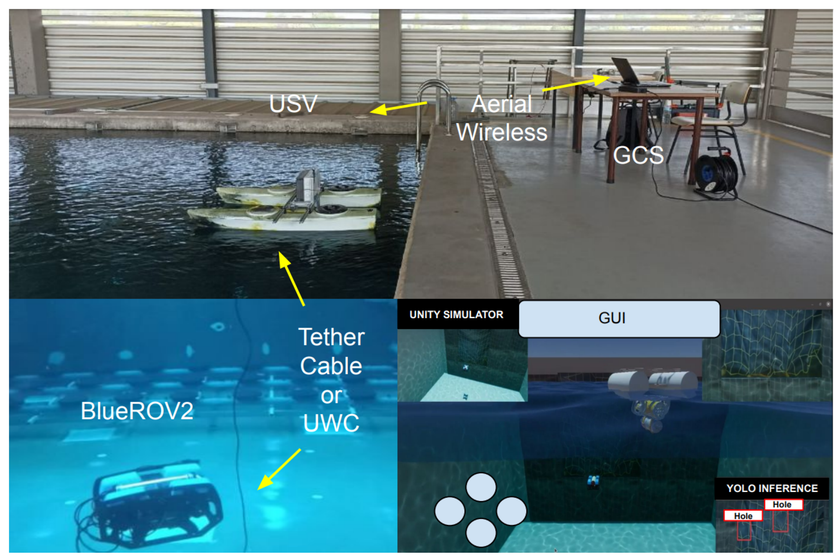
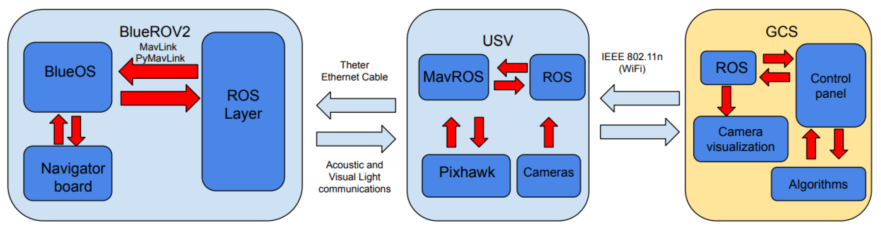
Communication plays a significant role in this application. The restrictions of underwater communications has led to the development of a floating platform or a unmanned surface vehicle (USV) that can serve as a link between the underwater robot and the ground station. Examples such as in [13], where a platform composed of USV swarms was used for real-time monitoring. That platform proposed a simultaneous multicommunication technology in a synchronized approach using LoRa, IEEE 802.11n (WiFi), and Bluetooth as a way of creating a multirange communication channel. It is important to note that it was designed to work in aquaculture environments. In this case, as in most of the works in the literature, the connection between the ROV and the surface vehicle was achieved with a tether cable, but some works such as [14] proved that optical and acoustic communications could be used to establish a wireless communication link between the underwater robot and the surface vehicle. We have performed several experiments to cope with underwater wireless communications (UWC). Acoustic and optical modems have been used to deal with this issue.

After introducing the robotic platform concept and going further into the specific inspection trajectory, some underwater localization concepts are presented. It is well known that robot localization in underwater environments is not as simple as in air, mainly because of the nonfunctioning of the Global Position System (GPS). Su et al. [15] conducted a review of the state of the art for underwater localization techniques, algorithms, and challenges. The authors pointed out that the most popular sensors used in small environments like a fish farm that allow the positioning of the robot are acoustic-based, including sonars, DVL, and USBL. Evidence of this can be found in the research conducted by Karlsen et al. [16], where an implementation of an autonomous mission control system for unmanned underwater vehicle operations in aquaculture showed the performance of the localization and trajectory tracking of an AUV using a DVL, an IMU, and an USBL as sensors. The last referenced work discussed the use of a finite state machine to ensure the complete inspection of the net and proved that even when the data from the DVL were not available for different parts of the trajectory, the AUV could complete the trajectory. Furthermore, Amundsen et al. [17] conducted research where an autonomous ROV inspection of aquaculture net cages was conducted using a DVL. In that application, the DVL was mounted on the bow of the ROV and the desired distance of the net was fixed to 2 m. The real experiments proved that the system followed a circular trajectory inside the net cage with some unknown ocean currents. However, the authors reported that velocity gains had to be low because of the noise measurements of the DVL.

Computer vision can be an alternative for positioning in confined environments. Evidence of this can be found in [18], where an intelligent navigation and control of an AUV for automated inspection of aquaculture net pen cages was developed using an optical camera. In that case, some markers were attached to the net. By using computer vision, an IMU, and a depth sensor, the AUV could develop an inspection trajectory. The pose of the AUV in a net fish cage was also estimated with a monocular camera in the work of C. Schellewald [19], where the input image was processed, and a squared region of interest was analyzed to detect regular peaks in the Fourier transform indicating the presence of a fish net. Once the fish net was detected and knowing the camera parameters, the position and orientation from the ROV to the net could be computed. The algorithm was tested with real fish-farm images containing salmons, and it could detect the region of interest and estimate the pose.

A. Duda et al. [20] proposed an algorithm for pose estimation, “the X junction”, which could detect the fish-net knots and their topology from camera images. After detecting the knots, the pose of the camera was estimated. The authors estimated the distance between the fish net, roll, pitch, and yaw with high accuracy at low distances (15 cm to 65 cm). A visual servoing scheme for autonomous aquaculture net pens’ inspection using a ROV was developed by Akram et al. [21]. The referenced work proposed the use of ropes attached to the net to estimate the relative position of the ROV between the net using computer vision. In a related context, ref. [22] introduced another monocular visual odometry work where the authors developed a real-time monocular visual odometry algorithm for turbid and dynamic underwater environments; the work compared the drift against the level of noise, depending on the turbidity of the water.

Most of these works that just depend on a monocular camera are sensible to low-light or high-turbidity water environments. To overcome that, Hoosang L. et al. [23] proposed an autonomous underwater vehicle control for fish-net inspection in turbid water environments. The authors trained a convolutional neural network (CNN) to predict the ideal net distance and the yaw set point to control the AUV.

Research involving net hole detection was conducted by Lin et al. [24], where an omnidirectional surface vehicle (OSV) for fish-net inspection was designed. The work also incorporated AI (artificial intelligence) planning methods for inspecting the whole net surface or focusing on an interesting area. The omnidirectional surface vehicle presented in [24] has an onboard camera with adjustable depth. That camera is used to take images from the net. In fish farms, nets can be larger than 20 m, and having only a surface vehicle limits the area of inspection; this means that having an underwater vehicle plays a significant role when inspecting the total net area.

Underwater imaging involves big challenges principally due to the environmental properties. Light scattering, light absorption, or water turbidity are some examples of phenomena that affect underwater images. To overcome this problem, traditional computer vision and deep learning techniques are applied. In [25], an underwater object detection review is presented. The most used architectures and detection algorithms are exposed in that work, such as CNNs, recurrent convolutional neural networks (RCNNs) and the You Look Only Once (YOLO) algorithm versions.

There are few works that use traditional computer vision methods like the Otsu threshold, the Hough transform, and convex hull algorithms that are used in [26] to reconstruct and detect holes in fish nets from a fish farm cage. The authors report a 79% of accuracy when examining net damages.

Deep learning techniques are the most used algorithms when detecting underwater objects, and these algorithms do not work the same in air as in underwater environments due to the environmental properties mentioned before. Works like [27] proposed a method for improving object detection in underwater environments based on an improved EfficientDet. That method modified the structure of the neural network and the results showed that the mean average precision (mAP) reached 92.82%. Also, the processing speed showed an increase reaching 37.5 FPS. This was important due to the onboard robot hardware characteristics.

As mentioned before, YOLO is one of the most used detection algorithms. In [28], the fifth version of that algorithm was tested and compared versus other algorithms such as faster RCNN or a fully convolutional one-stage (FCOS) method, and the results showed that the small version of YOLOv5 reached an mAP of 62.7% and around 50 FPS showing the best-combined results of the YOLOv5 versions.

1.3. Main Contribution

In this work, a robotic platform is presented, composed of a surface vehicle and an underwater vehicle embedded with artificial intelligence cooperating to develop an inspection task and hole detection in a controlled environment. The main contribution of this work lies in the integration and cooperation of underwater robotics. By employing control trajectory-tracking algorithms and a self-customized CNN to adjust inspection distances, the system is capable of inspecting cylindrical and planar-shaped nets. It can simultaneously detect holes within the net using a pretrained YOLOv8 algorithm with a dataset created from images captured in a real water-tank environment. This represents a step towards inspecting underwater environments, such as fish farms in this specific case, but it could also cover port facilities, large vessels, or marine reefs. Experiments were developed at a water tank of 12 × 8 × 5 m at the CIRTESU lab, UJI, Spain, where three different knot-size real fish nets were installed. These facilities allowed us to reduce the complexity of the environment and test algorithms in a previous stage. The experiments are a second stage and an extended version of the results presented at the international conferences Oceans 2023 and MarTech 2023, refs. [29,30], respectively. Also, a simulation scenario was developed to guarantee repeatability and increase the performance of the algorithms. The rest of the paper is organized as follows: Section 2 describes the foundations and methodological aspects. Section 3 exposes the experimental validation, where the experiments and the approach to follow are described. Section 4 shows the performance results and discussions of the experiments, and finally, Section 5 presents the conclusions of the presented work.

2. Foundations and Methodological Aspects

This section introduces the model of the surface and underwater vehicles. Then, the concept of convolutional neural networks is presented focusing on the object detection and classification problem. Finally, the classic proportional, integral, and derivative (PID) controller algorithm is described.

2.1. Vehicles’ Modeling

The most popular model in the literature for modeling marine vehicles is the one described by Fossen [31]. This model states that there is a reference system with respect to the Earth and another reference system with respect to the vehicle. There is also a way to express position, orientation, moments, and forces, which is endorsed by the Society of Naval Architects and Marine Engineers. The respective equations are shown below.

$$\eta ={(x,y,z,\phi ,\theta ,\psi )}^T$$

(1)

$$\upsilon ={(u,v,w,p,q,r)}^T$$

(2)

$$\tau ={(X,Y,Z,K,M,N)}^T$$

(3)

where $\eta$ represents the position and Euler rotation angles, $\upsilon$ represents linear and angular velocities, and the vector $\tau$ represents forces and moments. Figure 1 graphically depicts the reference system with respect to a surface vehicle. For a surface vehicle, the movements are restricted to a 2D plane. This means that only 3 degrees of freedom are taken into account (x, y, $\psi$); the same happens with the velocities (u, v, r) and forces (X, Y, N).

An underwater vehicle can be modeled in essentially the same way, but considering 6 DOFs. Equations (1)–(3) also express the position, orientation moments, and forces of an underwater robot. Regarding the motion dynamics of a vehicle, the model can be described using the Newton–Euler equilibrium laws. The adaptation for a maritime vehicle model is as follows:

$$M\dot{v}+C\left(v\right)\dot{v}+D\left(v\right)v+g\left(\eta \right)=\tau +w$$

(4)

$$\tau =B\ast u$$

(5)

In the above equation, the variable M represents the inertial mass matrix and added mass, C represents the rigid body matrix and added mass with Coriolis and centripetal values, D represents the hydrodynamic damping, B represents the position of the marine vehicle’s propellers, g represents the restoring forces, u represents the forces generated by the propellers, w represents disturbances due to ocean currents, and finally, $\tau$ represents the vector with the controller outputs.

Regarding the vehicle dynamics, two considerations are made: the vehicle is a rigid body, and the reference frame with the Earth is an inertial system. Based on these two principles, the rotational and translational movements that relate the vehicle’s reference system to the fixed system on Earth can be developed. This information was summarized from Chapter II of the book Guidance and Control of Ocean Vehicles [32].

2.2. Computer Vision and Intelligent Algorithms

In the area of computer vision and artificial intelligence, the CNN algorithm has been one of the most used techniques for object detection. A convolutional neural network is a type of artificial neural network that is commonly applied to analyze images. A CNN is basically composed of 4 types of layers: convolutional, pooling, flattening, and fully connected layers. The convolutional and pooling layers can be used more than once before using the flattening layer; this decreases the computational size and is one of the principles of a CNN. Figure 2 shows a diagram of a convolutional neural network.

The input of a CNN can be an RGB image; this image consists of three channels: red, green, and blue. Each channel has the same size as the image; the size of the image is determined by the number of width pixels by the height pixels. The value of each pixel depends on the color depth; in most cases, images have an 8-bit color depth, which means that the value of each pixel in each channel is in the range from 0 to 255. Using the 3D matrix of the image, a convolutional layer is applied.

The main objective of the convolutional layer is to extract the high-level features of the image. This layer consists of a smaller matrix, which is often called kernel or filter. Using this filter, a convolutional operation is computed on each channel of the 3D input image. The values of the pixels from the filter are called weights. In the training phase using the gradient descent method [33], the weights of the filter are adjusted to detect specific features of the desired detection object. After the convolutional operation, the size of the image has to be decreased using a pooling operation.

The pooling operation is responsible for reducing the size of the matrix. This reduces computational power by extracting the dominant features from the output of the convolutional layer. Similar to the convolutional layer, a mask is moved along a matrix, and at each step, a pooling operation is performed. There are two types of pooling, average and max-pooling. Average pooling consists of computing the average of the pixels where the pooling filter is located. The max-pooling operation takes the maximum value of the mask; this type of pooling is often more commonly used because it suppresses noise.

The flattening layer consists of processing a three-dimensional array that comes from a pooling layer and transforming it into a one-dimensional vector without losing any data. This output feeds a fully connected layer. It is important at that point that the size of the vector is not too large, as this would mean that the convolution and pooling layers are extracting the more important features.

Finally, the fully connected layer takes the output of the flatten layer as input and computes the output of each neuron of the next layer. In this type of neural network, each neuron is connected to every neuron of the previous layer. The weights associated with each connection are adjusted during the training phase. The purpose of this layer is to capture complex patterns and relationships in the data to make a prediction or decision. At the last layer of a fully connected neural network, the output is a probability of the detection of an object.

YOLO [34] is a real-time object detection and image segmentation model that is based on the convolutional neural network principle. It offers unparalleled performance in terms of speed and accuracy. This open-source algorithm offers detection, segmentation, pose estimation, tracking, and classification. For training this algorithm, there are different datasets available in the literature, but it is also possible to label a new dataset using tools like labelimg [35] or roboflow [36].

The YOLO algorithm has different versions; Ultralytics’s available versions are from YOLOv3 to YOLOv8. The main differences between YOLOv8 and the previous versions are an improvement in the feature extraction, object detection performance, accuracy, balance between accuracy and speed, and a variety of pretrained models, as its documentation states [37]. The 8th version consists of different sizes: nano, small, medium, large, and extralarge. Each size has different performance values, so the balance between speed and accuracy has to be taken into account when selecting a model.

2.3. Control Algorithms

A PID controller is a linear controller. This means that the performance for first-order systems is good, but for high-order nonlinear systems, the error can increase considerably. The controller consists of 3 parts: The proportional part multiplies the position error by a constant. The derivative part multiplies the velocity error; this part of the controller is indispensable when dealing with trajectory-tracking algorithms. Finally, the integral part of the controller tries to reduce the steady-state error. Equation (6) shows the control law of a PID controller.

$$\tau =k_p\ast e_p\left(t\right)+K_d\ast e_v\left(t\right)+k_i{\int }_0^t{e}_p\left(t\right)\mathrm{d}t$$

(6)

where ${\mathit{K}}_{\mathit{p}}$, ${\mathit{K}}_{\mathit{d}}$, and ${\mathit{K}}_{\mathit{i}}$ represent the proportional, derivative, and integral gain, respectively. ${\mathit{e}}_{\mathit{p}}$ means the position error, ${\mathit{e}}_{\mathit{v}}$ is the velocity error, and finally, $\tau$ represents the control action. Figure 3 shows a block diagram of a feedback controller.

3. Experimental Validation

In this section, an overview of the fish-net inspection problem and its proposed solution is presented. The development of the solution includes a detailed description of its components. Components such as the surface vehicle, autonomous underwater vehicle, and ground station are described. Finally, the “approach to follow” subsection describes the strategy and methodology employed to tackle the presented problem, detailing the step-by-step process adopted for its resolution. This subsection also includes the communications, computer vision, and artificial intelligence algorithms utilized for robot pose control and hole detection.

The proposed algorithms in this work were tested in a controlled environment where underwater currents, wind, waves, turbid water, significant variations in light, and objects obstructing the camera could affect algorithm performance. To test these algorithms, reducing the complexity of an environment like a fish farm was necessary to make progress. However, these feedback-based algorithms exhibited a certain degree of robustness when faced with the aforementioned phenomena. Proof of this is that the artificial vision algorithms for hole detection and net distance estimation were trained under different lighting conditions, making the algorithm more robust. In the future work section, a research line is described to extend these algorithms to a more challenging environment, such as aquaculture facilities in their final stage.

3.1. Experimental Setup

3.1.1. Net Inspection Problem

The problem we aimed to address is the inspection of a fish-farm net. This work focused on a specific section of the net, for the purposes of implementation in a water tank. To tackle this challenge, we propose an integrated system with a surface robot, an underwater robot, a GCS, and a user interface. A diagram of the main building blocks (hardware and software) integrating the complete system under development can be observed in Figure 4.

The primary objective was to have an underwater robot able to execute an inspection trajectory through the net, while simultaneously running a hole detection algorithm. All data collected by the underwater robot were transmitted using an umbilical cable to the surface robot; subsequently, the surface robot transmitted all the data to the ground control station (GCS). At the GCS, the user had control over the inspection process, which was a blend of automatic and remote operations.

3.1.2. Surface Vehicle

The surface vehicle used in this work was a new version of that presented in [38]. This surface vehicle had 4 thrusters similar to the original used in the previous version, which allowed omnidirectional movement. Also, this vehicle was embedded with two low-light HD USB cameras, Sony IMX322/323 (Sony, 1 Chome-7-1 Konan, Minato City, Tokyo 108-0075, Japan) one underwater, and the other one at the surface. The vehicle is shown in Figure 1.

3.1.3. Underwater Vehicle

The underwater robot used in the experiments was the BlueROV2 in its heavy configuration, (BlueRobotics Inc., 2740 California St, Torrance, CA 90503, USA [39]). This configuration allowed us to have a 6-DOF control of the robot. Communication with the robot was established using a tether cable, the Mavlink protocol [40], and the PyMavlink library [41]. Figure 5 shows the body and the earth frame of the underwater vehicle as in [42], where the author explains the kinematic and hydrodynamic model considering 6 degrees of freedom.

3.1.4. Ground Control Station

The GCS consisted of a MSI GE 76 RAIDER (901 Canada Court, City of Industry, CA, USA) with Ubuntu 20.04 installed, Intel i7 processor, 16 GB of RAM, and QgroundControl software version v4.2.4 [43], ROS noetic, and the PyMavlink library. Here, the user interface can help the operator visualize the cameras and telemetry data and allow them to intrude into the loop and take decisions. The user interface is under development.

3.2. Simulation Environment

A simulation was created using the 2023.1 HDRP version of the Unity game engine [44] (30 3rd Street, San Francisco, CA, USA) and the robotic package. The simulation included a real-dimension 3D model of the water tank from the CIRTESU lab, a 3D model of the 2 robots (surface and underwater), and pictures from a real underwater environment. Figure 6 presents the simulation environment.

Communications with the simulation were based on the Unity Robotics Hub. This means that the simulation published the sensors of the robot via ROS topics, and the robots navigated using a command velocity ROS topic. It is important to mention that the simulation did not include any disturbances.

The purpose of the simulation was to test all the elements needed to develop the inspection task, such as net distance control, trajectory tracking, hole detection, and hole positioning. In conclusion, a simulation was developed in which the virtual robot inspected the net, maintaining a desired distance, while simultaneously following an inspection trajectory and executing a hole detection algorithm.

3.3. CIRTESU Water Tank

The experiments were conducted in the CIRTESU water tank, which measures 12 × 8 × 5 m. In this controlled environment, three fish nets were installed for the study, each one with different knot distances (30, 20 and 10 mm). Nets were courtesy of AVRAMAR, an aquaculture company, with several fishing farms along the Valencian coast, including Burriana, near the UJI Campus. Figure 7 shows the nets used.

Figure 8 shows the complete setup, where a 2 × 2 m piece of the net was positioned at the center of the tank, and both surface and underwater robots performed the inspection task.

Three experiments were devised in the water tank: hole detection, hole positioning, and net distance keeping. These three experiments are explained next.

3.3.1. Hole Detection

In this experiment, the hole detection algorithm was evaluated in the real tank. The robot tried to detect ten holes of different sizes in each of the three nets, situated at three different distances.

3.3.2. Hole Positioning

For this test, the robot had to position itself in front of the hole; a proportional feedback controller was used. The x and y axis were controlled using the pixels of the camera, and the distance between the robot and the hole was controlled using the area of the hole.

3.3.3. Net Distance Estimation

In this test, a convolutional neural network predicted if the robot’s position was far or close to the net. This helped with the inspection trajectory, because if the distance was too close, the inspection would be time-consuming, but if the distance was too far, the hole detection algorithm would not be accurate.

3.4. Approach to Follow and Algorithms

Using the robotic platform described in the experimental setup subsection, the underwater robot had to inspect the net while the surface vehicle provided a communication link to the control station. To develop this task, communications, computer vision, position control, and intelligent algorithms were needed. In the rest of this subsection, these algorithms and communications are explained.

3.4.1. Communications

Basically, all the components of the platform used ROS. The ground station used ROS noetic, and the surface vehicle used ROS melodic and the MavROS package, which allowed communication between the Raspberry Pi and the Pixhawk (the flight controller). Communications with the BlueROV2 were different, principally because that version of the BlueROV2 used BlueOS, which is an operative system that is installed over the Raspbian OS of the Raspberry Pi. Thus, to be able to communicate with the robot, the PyMavlink library was used. Figure 9 shows a diagram of the communications of the robotic platform.

Tests related to UWC were conducted simultaneously with the tether cable. As physical and link layers, we had two different communication media (parallel to the tether), an acoustic modem Evologics Wise S2R 18/34 [45], which can perform at a bandwidth of up to 13 Kbps with range distances of up to 3500 m, and an optical modem Luma X from Hydromea [46], which works up to 10 Mbps at a maximum distance of 50 m. The idea was to perform the inspection tasks using low-bandwidth communications by means of the acoustic modem. When a high bandwidth was required, we could switch to the optical fast-communication system; in such a case, the BlueROV2 and the surface vehicle had to move close to each other, at a maximum of around 5 m.

A region of interest was used to adapt the size of the images sent by the BlueROV2 according to the available bandwidth; this adapted the quantity of data to be sent according to the available bandwidth.

Communications between the surface vehicle and the ground station were performed by means of a high-speed WiFi connection, although several other alternatives are available.

3.4.2. Net Distance Keeping

A previous version of this work was presented at the International Congress Oceans 2023, where a convolutional neural network was trained to identify if the robot was close or far to the net, only using the image from the camera. The architecture of that neural network was custom-designed specifically for the current problem, with the goal of achieving the highest possible estimation frequency without sacrificing performance. This customization was intended to increase the performance of the controller. On the other hand, for the task of detecting holes, a high precision in hole detection is crucial. That is why a detection algorithm such as YOLO was employed. Basically, a CNN was built using the TensorFlow library and Keras. The architecture of the neural network started with an input and a normalization layer, followed by a series of 2D convolutions and max-pooling layers. The architecture used the rectified linear unit (Re-LU) as the activation function. Finally, a flattened layer was followed by two dense layers: 64 neurons in the first and an output neuron using a sigmoid function as an activation function. This means that the final layer produced an output value ranging between 0 and 1, which reflected the distance towards the net. A prediction of 0 indicated that the robot was near the net and a prediction closer to 1 meant that the robot was far away from the net. In simple terms, this value provided an estimation of how far or close the robot was to the net. Figure 10 shows a block diagram of the net’s architecture.

The neural network was trained over 15 epochs and some features are:

• A total of 849 total images, captured from different nets and distances.
• A total of 680 training images, 169 validation images.
• A total of 200 testing images, taken at different times and in different conditions.
• Different lighting conditions.
• Bach size of 32.
• Two classes, far and close.
• Training accuracy of 97%.
• Validation accuracy of 94%.
• Testing accuracy of 92%.
• Testing loss of 0.2560.

The dataset was created using images from a real environment. Random flips and rotations were used as data augmentation techniques, and no synthetic data were used in the training process. Nonetheless, the CNN results demonstrated its usability in both simulation and real environment. The results of the training over the epochs can be seen in Figure 11. In the graph, the validation accuracy and the validation loss fluctuated with respect to the training accuracy and training loss. However, after 15 epochs, the validation loss decreased from 0.9 to 0.2, and the validation accuracy achieved more than 94%.

3.4.3. Hole Detection

This subtask has to run parallel to the trajectory inspection. First, a dataset was created with images of the experimental setup. Some characteristics of the dataset are mentioned below:

• A total of 847 images with different holes and different nets.
• Different light conditions, some of them using the lights of the underwater robot and others without the lights.
• Data augmentation such as rotations, crop, blur, and noise was applied.
• More than 2000 images for the training set (after data augmentation) and 170 images for the validation set.

The dataset can be accessed using the link (accessed on 24 December 2023): https://universe.roboflow.com/salvador-lpez-barajas/realholes. Second, the detection algorithm used was YOLOv8 in its nano version. This version was chosen because the detection model had to run on a Jetson nano, which can be embedded in the robot platform.

The most important training parameters are described in

Table 1. Learning strategy.

Parameter	Value
Optimizer	SGD
IOU	0.7
LR0	0.01
LRF	0.01
Momentum	0.937
Weight decay	0.0005
Dropout	0.0

, and the training was based on the default values of the next colab notebook (accessed on 24 December 2023) https://github.com/roboflow/notebooks/blob/main/notebooks/train-yolov8-object-detection-on-custom-dataset.ipynb. Data from 100 epochs of training and an image size of 640 showed that the training losses and the validation losses graphs were quite similar; there was just a small increase in the validation. The precision and recall metrics showed the performance of the algorithm when detecting net holes, with values around 90%. Finally, the mAP50 and mAP50-95 pointed out that the model’s average precision at the 0.5 intersection over union rate (IoU) was high, but it decreased significantly when the IoU increased from 0.50 to 0.95. Graphs are presented in Figure 12, where the training and validation losses of the bounding box, class, and distribution focal loss demonstrate the learning process, and the metrics exhibit the performance of the algorithm.

3.4.4. Hole Positioning

Once a hole is detected, the next step is to fix it. However, the previous step before the manipulation task is hole positioning, which consists of moving the robot autonomously and positioning it in front of the hole. Using the pixel coordinates and the area of the hole as set points, a feedback control was implemented. In this case, the image used for this task was a 640 × 480 image, so the set point was fixed at (320, 240) pixels, and the distance from the net was controlled using the area of the bounding box. The position was measured with an ArUco marker attached beside the hole. Other sensors such as a DVL or a sonar can be used to measure the distance to the net; in future work, these sensors will be used to design a position controller using nonlinear control methods. Figure 13 shows how the ArUco marker was attached to the net.

The controller was a proportional feedback controller; this controller was chosen as a proof of concept, but in future work, nonlinear control techniques such as sliding modes or neural networks will be used to increase the robustness of the controller. Some of the considerations when developing the experiment were:

• The robot was in the stabilizing mode of the QGround Control app.
• The communication with the robot was performed using Mavlink and a different endpoint from the one of Qground Control.
• The maximum control signal was from the 1415 to 1585 ESC PWM input value (microseconds).
• Because of the nature of the problem, small gains were applied.

The parameters of the controller are shown in

Table 2. PID parameters of the hole-positioning algorithm.

Axis of Movement	Proportional Gain	Set Point
Depth	0.01	320
Yaw	0.03	0
Lateral axis	0.01	240
Frontal axis (hole distance)	0.00005	40,000

.

Once the controller gain was computed, it was limited to a range between −1 and 1; finally, this value was multiplied by 85 (the controller range was from 1415 $\mathsf{\mu }$s to 1585 $\mathsf{\mu }$s).

4. Results

This section is divided into the different subtasks that constitute the inspection operation. First, the UWC results are described. Secondly, the hole detection algorithm results are presented. Then, a subtask where the robot position itself automatically in front of the hole is presented; this represents the step before performing a manipulation task to repair the hole. Repairing the hole was out of the scope of this work. After that, the results of the net distance estimation algorithms are presented. Finally, videos from the simulator are presented in the trajectory control subsection; these videos represent an overview of an inspection operation of a fish-farm net with all the tools mentioned before.

4.1. Underwater Wireless Communication

A multimodal communication system was tested in parallel to the tether cable to communicate with the BlueROV2 and the surface vehicle. The acoustic modem was used during the net inspection, and when a high bandwidth was required, the BlueROV2 and surface vehicle came closer to each other in order to be able to use the optical modem. In our experiments, we obtained an average of 549.36 bps using the acoustic modem, which was far from the 13 kbps that the builder claimed. This lack of bandwidth may have been caused by the refraction in the water tank. Regarding the optical modem, we reached speeds up to 5 Mbps with distances of 9 m and clear water. A more detailed description of the low-level communications can be found in [47].

Regarding semantic compression, the images were compressed using the JPEG 2000 standard, which allowed us to reduce the dimension and quality of the images. According to the available bandwidth, an algorithm performed the compression to send images at a specified ratio (fps) specified by the system operator. In

Table 3. Image size, in bytes, according to the percentage of compression in dimension and quality.

	20% Dimension	50% Dimension	90% Dimension	100% Dimension
5% Quality	317	474	845	965
20% Quality	416	945	2099	2444
60% Quality	627	1986	5248	6628
100% Quality	2828	15,675	48,098	41,451

, the different sizes of images are shown according to their dimension and quality. The image size varied from its maximum size of 41,451 bytes to 317 bytes with maximum compression in size and quality.

Using the multimodal communications model and semantic compression, we developed an UWC platform which dynamically took advantage of the available bandwidth in order to communicate with the BlueROV2 and the surface vehicle. In the worst-case scenario, using the acoustic modem, we could transfer a low-dimension and low-quality image every five seconds, but in normal situations, one frame per second was transmitted, which was more than enough for the inspection tasks.

4.2. Hole Detection

To test the algorithm, 10 different hole sizes were created in each fish net. The hole sizes ranged from a single broken mesh to a final horizontal hole spanning 10 meshes. Then, the robot inspected the net at three different distances: near, medium, and far distances. The near distance was approximately 70 cm, while the medium distance was around 150 cm, and the far distance extended to around 300 cm. After that, the confidence level of detection was measured for each hole.

Table 4. Detection confidence of holes at the 10 mm knot size net.

Hole Size (Broken Meshes)	Near Distance (70 cm)	Medium Distance (150 cm)	Far Distance (300 cm)
1	No detection	No detection	No detection
2	0.49	0.55	No detection
3	0.49	0.51	No detection
4	0.47	0.66	0.59
5	0.70	0.65	No detection
6	0.66	0.69	0.58
7	0.73	0.70	0.62
8	0.69	0.70	0.66
9	0.71	0.69	0.72
10	0.82	0.73	0.66

,

Table 5. Detection confidence of holes at the 20 mm knot size net.

Hole Size (Broken Meshes)	Near Distance (70 cm)	Medium Distance (150 cm)	Far Distance (300 cm)
1	No detection	No detection	No detection
2	0.48	No detection	No detection
3	0.53	No detection	No detection
4	0.56	0.46	0.50
5	0.56	0.50	0.61
6	0.62	0.58	0.66
7	0.67	0.59	0.64
8	0.62	0.49	0.49
9	0.72	0.66	0.69
10	0.77	0.47	0.57

and

Table 6. Detection confidence of holes at the 30 mm knot size net.

Hole Size (Broken Meshes)	Near Distance (70 cm)	Medium Distance (150 cm)	Far Distance (300 cm)
1	No detection	No detection	No detection
2	0.50	0.5	0.48
3	No detection	0.53	No detection
4	0.67	0.59	0.56
5	0.66	0.54	0.62
6	0.69	0.56	0.55
7	0.77	0.70	0.74
8	0.74	0.59	0.63
9	0.82	0.77	0.63
10	0.87	0.79	0.61

display the results of the detection algorithm at various distances and with different hole sizes. It can be observed that the precision decreased as the robot moved farther away from the net when detecting small holes; in other words, the confidence increased when the detection was performed at near distances. Larger holes could be detected easily at larger distances, but this also depended on the water and lighting conditions.

Results showed that the larger the size of the hole, the more confident the algorithm, but this could also be affected by the background. In our case, the walls of the water tank had some white stains, and in some frames, this influenced the predictions. The results also showed that there were some holes that were not detected by the algorithms; these holes were mainly small holes at larger distances. This shows where the limit lies in terms of the distance at which the inspection must be carried out. It is important to remember that while inspecting the net from a greater distance will reduce the route and inspection time, the precision with which the algorithm detects holes will also decrease. That is why finding a balance is crucial. To detect holes from a greater distance, one option can be to increase the camera quality and develop a larger dataset. However, this would also increase the time for each prediction, decreasing the speed at which the robot can perform the inspection. Figure 14 shows three images from different distances from the 20 mm knot distance net.

4.3. Hole Positioning

Once the hole is detected, the robot has to position itself autonomously at a manipulation distance. To start the experiment, the robot was located at a distance where the hole could be identified, then the autonomous positioning algorithm was launched. Figure 15 shows a graph of the position of the robot, in centimeters, with respect to the hole. And, Figure 16 shows the control in pixels over time.

The graphs indicate that the control system was stable. When the robot came closer to the hole, it is important to note that the accuracy of the x and y axes did not decrease; instead, it improved. However, the area estimation varied considerably, primarily due to inaccuracies in the neural network’s bounding-box predictions. Consequently, this led to some instability in the distance with the net. The results also demonstrated a significant reduction in distance from 3 m to approximately 17 cm (when the distance controller was turned on, after 20 s of centering the hole), within which a robotic arm could be utilized to perform the hole-repairing task. The videos of the experiment can be found at the next links (accessed on 24 December 2023); in these videos, the ArUco marker was removed. External view: https://drive.google.com/file/d/1R3C0NmwVhxG_ZHJxNoIzJUI_qfcwc3O7/view?usp=sharing Robot Camera: https://drive.google.com/file/d/1ia7NRBBDcCv5CZaaBUPB_67LnHAgrmRk/view?usp=sharing.

4.4. Net Distance Estimation

Figure 17 shows two predictions of the convolutional neural network.

A proportional controller was used to maintain the position of the underwater robot with respect to the net. The set point of the controller was set at 0.5 (approximately 80 cm) and the proportional gain was set to 0.2 in the simulator and 200 in the real robot. This means that the PWM range from the MAVLink channel was from 1400 $\mathsf{\mu }$s to 1600 $\mathsf{\mu }$s assuming that the maximum error could be $\pm 0.5$ as a result of the output of the CNN (1500 $\mathsf{\mu }$s was the nonmovement value). The results of this experiment are shown in the next Figure 18.

4.5. Trajectory Control

4.5.1. Simulation Planar Trajectory

A simulation with a PID control trajectory tracking was designed to test the algorithm of net-distance control and hole detection. This trajectory consisted of a horizontal movement and then a vertical motion. For this test, the Unity simulation was used, and a PID controller was designed using Python and ROS. The constants of the PID controller are shown in

Table 7. PID parameters of planar prototype of the net cage trajectory.

Axis of Movement	P	I	D
Depth	0.3	0.1	0.1
Yaw	0.03	0	0
Lateral axis	0.8	0.1	0.3
Net distance	0.2	0	0

.

A video of the results and the future aim of the whole robotic platform can be found at the link (accessed on 24 December 2023): https://drive.google.com/file/d/1y8joBCl2bz41zCEtu2Q23mXy3KWAYcIW/view?usp=drive_link.

4.5.2. Trajectory on the Prototype of the Net Cage

This test was conducted on the simulator, and it is important to mention that there were no disturbances applied, but the trajectory in the x and y coordinates was influenced by the net-distance algorithm. Figure 19 shows the complete trajectory, in red, the desired set-point trajectory and in blue, the real trajectory. The depth controller showed great performance and the cylindrical trajectory could be appreciated.

The phenomenon of the movement due to the net-distance algorithm can be seen in Figure 20, where each iteration of the circular movement was a little different than the other. This drift was mainly because of the added noise of the simulated IMU; this caused an error in the orientation’s proportional controller. This drift in the trajectory was overcome by the net-estimation algorithm, which is one of the main contributions of this article.

Figure 21 shows the position error of the cylindrical trajectory, where the maximum error was about 60 cm.

This experiment is where all the previous net inspection experiments join, and from the results presented here, it is clear that this approach can be followed and improved to achieve a robust net inspection system. This is a step in the direction of developing a complete, autonomous, untethered robot capable of inspecting the entire area of a net cage while simultaneously making intelligent decisions. This means that the robot can autonomously inspect a portion of a net cage using a control trajectory and an obstacle-avoidance algorithm (to prevent entanglement or collisions). Subsequently, it can navigate to a safe data transfer location near the surface vehicle, and finally, using the VCL link, it can transfer all the information gathered during the inspection. This process can be repeated as many times as necessary. The video of this experiment is available at the link (accessed on 24 December 2023): https://drive.google.com/file/d/1TOAPJGtmtLUAWRS785P4kL7LrQSDdd5Y/view?usp=drive_link.

4.6. Discussion

Referring to hole detection, the results validate that the use of a convolutional neural network, such as YOLO, allows the detection of different holes at different distances from the net. However, detecting different types and sizes of holes requires a large quantity of training data. These data can be gathered from a controlled environment like the one presented in this work, but it would be beneficial if it could be for real holes at a real fish farm. Also, other anomalies can be detected with the same CNN; detecting the level of deterioration can be an example of taking the detection algorithm to the next level.

Regarding the hole positioning, the results prove that the robot was stable while staying in position in front of the hole. However, it is important to mention that the experiment was conducted in a controlled environment without any disturbances, such as water currents or fish swimming around. For this experiment, the controller used was a proportional feedback controller, but in a more realistic environment, a nonlinear controller will be needed. This is important when performing the manipulation and repairing the hole.

Concerning the net distance keeping using CNN experiments, the results show that our algorithm is capable of adjusting the set-point inspection distance. our algorithm makes sure that the quality of the captured images is correct. However, future experiments will include a stereo camera to measure the net distance. Using a stereo camera does not mean that the proposed algorithm will be discarded; quite the opposite, the algorithm will be improved to detect if the robot orientation is not perpendicular to the net. By mixing the distance measured using the stereo camera, the orientation, and set-point adjustment, the robot pose with respect to the net will be improved.

The autonomous underwater vehicle trajectory was a task that was tested in the simulation and in a simplified version in the tank. To develop a complete trajectory, a positioning system such as a DVL is strongly needed. Positioning can also be improved by combining the DVL sensor with an USBL, but the system has to be tested to make sure there are no acoustic reflections because of the environment. Additionally, the robot must have a reliable IMU, and an orientation controller has to be developed to adjust the orientation of the robot to be orthogonal to the net.

Using UWC could help eliminate the use of a tether cable, preventing it from snagging on the cages. We dealt with the low bandwidth of acoustic modems by using semantic perception and a high-speed low-distance optical modem.

5. Conclusions

A robotic platform consisting of an autonomous underwater vehicle connected to a surface vehicle either through a tether cable or underwater wireless communications was proven to be a highly effective method when developing an underwater inspection. In this setup, the USV established a communication link between the GCS and the AUV while conducting inspections of the net.

The results suggest that YOLOv8 is a robust algorithm for detecting holes in fish-farm nets. This statement holds true under favorable lighting conditions and moderate water turbidity, enabling the underwater robot to capture high-quality images. The findings revealed that the algorithm effectively identified larger holes (exceeding 15 cm) at a moderate distance of approximately 150 cm. The detection distance decreased to around 70 cm for smaller holes (less than 15 cm). A controller was designed to maneuver the AUV in alignment with the hole using a hole detection algorithm. This experiment demonstrated the robot’s ability to stabilize itself at a manipulation distance of 17 cm from the hole. In an undisturbed scenario, the hole could be precisely centered within the image.

Furthermore, the net distance estimation algorithm, coupled with the proportional controller, demonstrated the ability to regulate the distance between the autonomous underwater vehicle and the net. With a set point of 0.5, the dataset indicated a controlled distance of approximately 80 cm, providing sufficient proximity to conduct inspections and detect small holes effectively. Finally, the simulated trajectories validated the net distance estimation algorithm’s versatility in inspecting both planar and cylindrical nets, showcasing its capability to adjust distances as needed.

The UWC system, composed of two communication media, acoustic and optical, was very challenging. When a high speed was required, the optical modem could be used at the cost of repositioning both the BlueROV2 and the surface vehicle. Otherwise, in normal inspecting situations, semantic perception allowed us to take advantage of the whole acoustic modem bandwidth.

Future work can be divided into different research lines.

• Improving the pose and inspection trajectory control using a DVL and nonlinear control techniques such as sliding modes.
• Developing a user interface.
• Improving the UWC and integrating the multimodal communications with semantic compression in ROS.
• Repairing the hole using a manipulation arm.

Regarding the hole repairing, it is worth noting that the IRS-Lab at UJI has developed over the last 15 years a strong know-how in the underwater robotic manipulation context (e.g., the TWINBOT project [48]). The main goal of this field is to find a way to repair a hole using the Reach Alpha manipulator from Reach Robotics [49]. Figure 22 shows the experimental setup and one of the first underwater manipulation tests.

References

1. Hosomi, R. Seafood Consumption and Components for Health. Glob. J. Health Sci. 2012, 3, 72–86. [Google Scholar] [CrossRef] [PubMed]
2. FAO. The State of World Fisheries and Aquaculture 2022—Towards Blue Transformation; FAO: Rome, Italy, 2022. [Google Scholar] [CrossRef]
3. Overview of EU Aquaculture (Fish Farming). Available online: https://oceans-and-fisheries.ec.europa.eu/ocean/blue-economy/aquaculture/overview-eu-aquaculture-fish-farming_en#aquaculture-production (accessed on 7 July 2023).
4. Cámara, A.; Santero-Sánchez, R. Economic, Social, and Environmental Impact of a Sustainable Fisheries Model in Spain. Sustainability 2019, 11, 6311. [Google Scholar] [CrossRef]
5. Holen, S.M.; Utne, I.B.; Holmen, I.M.; Aasjord, H. Occupational safety in aquaculture—Part 1: Injuries in Norway. Mar. Policy 2018, 96, 184–192. [Google Scholar] [CrossRef]
6. Holen, S.M.; Utne, I.B.; Holmen, I.M.; Aasjord, H. Occupational safety in aquaculture—Part 2: Fatalities in Norway 1982–2015. Mar. Policy 2018, 96, 193–199. [Google Scholar] [CrossRef]
7. Autonomous Robots Will Change the Fish Farming Industry. Available online: https://www.innovationnewsnetwork.com/autonomous-robots-will-change-the-fish-farming-industry/11682/ (accessed on 24 December 2023).
8. Diving Safety. Available online: https://thefishsite.com/articles/diving-safety (accessed on 24 December 2023).
9. Ohrem, S.J.; Kelasidi, E.; Bloecher, N. Analysis of a novel autonomous underwater robot for biofouling prevention and inspection in fish farms. In Proceedings of the 28th Mediterranean Conference on Control and Automation (MED), Saint-Raphaël, France, 16–18 September 2020; pp. 1002–1008. [Google Scholar] [CrossRef]
10. Vasileiou, M.; Manos, N.; Kavallieratou, E. IURA: An Inexpensive Underwater Robotic Arm for Kalypso ROV. In Proceedings of the 2022 International Conference on Electrical, Computer, Communications and Mechatronics Engineering (ICECCME), Malé, Maldives, 16–18 November 2022; pp. 1–6. [Google Scholar] [CrossRef]
11. Amran, I.Y.; Isa, K. Modelling Analysis of Spherical Underwater Robot for Aquaculture Biofouling Cleaning. In 12th National Technical Seminar on Unmanned System Technology 2020; Lecture Notes in Electrical Engineering; Springer: Singapore, 2020; Volume 770. [Google Scholar] [CrossRef]
12. Osen, O.L.; Leinan, P.M.; Blom, M.; Bakken, C.; Heggen, M.; Zhang, H. A Novel Sea Farm Inspection Platform for Norwegian Aquaculture Application. In Proceedings of the OCEANS 2018 MTS/IEEE Charleston, Charleston, SC, USA, 22–25 October 2018; pp. 1–8. [Google Scholar] [CrossRef]
13. Sousa, D.; Hernandez, D.; Oliveira, F.; Luís, M.; Sargento, S. A Platform of Unmanned Surface Vehicle Swarms for Real Time Monitoring in Aquaculture Environments. In Proceedings of the OCEANS 2010 IEEE SYDNEY, Sydney, NSW, Australia, 24–27 May 2010; pp. 1–6. [Google Scholar] [CrossRef]
14. Farr, N.; Bowen, A.; Ware, J.; Pontbriand, C.; Tivey, M. An integrated, underwater optical/acoustic communications system. Sensors 2019, 19, 4695. [Google Scholar] [CrossRef]
15. Su, X.; Ullah, I.; Liu, X.; Choi, D. A Review of Underwater Localization Techniques, Algorithms, and Challenges. Hindawi J. Sens. 2020, 2020, 6403161. [Google Scholar] [CrossRef]
16. Karlsen, H.Ø.; Amundsen, H.B.; Caharija, W.; Ludvigsen, M. Autonomous Aquaculture: Implementation of an autonomous mission control system for unmanned underwater vehicle operations. In Proceedings of the OCEANS 2021, Porto, San Diego, CA, USA, 20–23 September 2021; pp. 1–10. [Google Scholar] [CrossRef]
17. Amundsen, H.B.; Caharija, W.; Pettersen, K.Y. Autonomous ROV Inspections of Aquaculture Net Pens Using DVL. IEEE J. Ocean. Eng. 2022, 47, 1–19. [Google Scholar] [CrossRef]
18. Livanos, G.; Zervakis, M.; Chalkiadakis, V.; Moirogiorgou, K.; Giakos, G.; Papandroulakis, N. Intelligent Navigation and Control of a Prototype Autonomous Underwater Vehicle for Automated Inspection of Aquaculture net pen cage. In Proceedings of the 2018 IEEE International Conference on Imaging Systems and Techniques (IST), Krakow, Poland, 16–18 October 2018; pp. 1–6. [Google Scholar] [CrossRef]
19. Schellewald, C.; Stahl, A.; Kelasidi, E. Vision-based pose estimation for autonomous operations in aquacultural fish farms. IFAC-PapersOnLine 2021, 54, 438–443. [Google Scholar] [CrossRef]
20. Duda, A.; Schwendner, J.; Stahl, A.; Rundtop, P. Visual pose estimation for autonomous inspection of fish pens. In Proceedings of the OCEANS 2015-Genova, Genova, Italy, 18–21 May 2015; pp. 1–6. [Google Scholar] [CrossRef]
21. Akram, W.; Casavola, A.; Kapetanović, N.; Miškovic, N. A Visual Servoing Scheme for Autonomous Aquaculture Net Pens Inspection Using ROV. Sensors 2022, 22, 3525. [Google Scholar] [CrossRef] [PubMed]
22. Ferrera, M.; Moras, J.; Trouvé-Peloux, P.; Creuze, V. Real-Time Monocular Visual Odometry for Turbid and Dynamic Underwater Environments. Sensors 2019, 19, 687. [Google Scholar] [CrossRef] [PubMed]
23. Lee, H.; Jeong, D.; Yu, H.; Ryu, J. Autonomous Underwater Vehicle Control for Fishnet Inspection in Turbid Water Environments. Int. J. Control Autom. Syst. 2022, 20, 3383–3392. [Google Scholar] [CrossRef]
24. Lin, T.X.; Tao, Q.; Zhang, F. Planning for Fish Net Inspection with an Autonomous OSV. In Proceedings of the 2020 International Conference on System Science and Engineering (ICSSE), Kagawa, Japan, 31 August–3 September 2020; pp. 1–5. [Google Scholar] [CrossRef]
25. Syed, F.; Showkat Ahmad, P.; Ghulam Jeelani, Q. Underwater object detection: Architectures and algorithms—A comprehensive review. Multimed. Tools Appl. 2022, 81, 20871–20916. [Google Scholar] [CrossRef]
26. Betancourt, J.; Coral, W.; Colorado, J. An integrated ROV solution for underwater net-cage inspection in fish farms using computer vision. SN Appl. Sci. 2020, 11, 1946. [Google Scholar] [CrossRef]
27. Jia, J.; Fu, M.; Liu, X.; Zheng, B. Underwater Object Detection Based on Improved EfficientDet. Remote Sens. 2022, 14, 4487. [Google Scholar] [CrossRef]
28. Wang, H.; Sun, S.; Wu, X.; Li, L.; Zhang, H.; Li, M.; Ren, P. A YOLOv5 Baseline for Underwater Object Detection. In Proceedings of the OCEANS 2021, Porto, CA, USA, 20 September 2021; pp. 1–4. [Google Scholar]
29. López-Barajas, S.; González, J.; Sandoval, P.J.; Gómez-Espinosa, A.; Solis, A.; Marín, R.; Sanz, P.J. Automatic Visual Inspection of a Net for Fish Farms by Means of Robotic Intelligence. In Proceedings of the OCEANS 2023-Limerick, Limerick, Ireland, 5–8 June 2023; pp. 1–5. [Google Scholar] [CrossRef]
30. López Barajas, S.; González, J.; Solis Jiménez, A.; Gómez Espinosa, A.; Marín Prades, R.; Sanz Valero, P.J. Towards automatic hole detection of a net for fish farms by means of robotic intelligence. Instrum. Viewp. 2023, 22, 76. [Google Scholar]
31. Fossen, T.I. Introduction. In Handbook of Marine Craft Hydrodynamics and Motion Control; John Wiley & Sons, Ltd.: Chichester, UK, 2011; pp. 3–12. ISBN 9781119994138. [Google Scholar]
32. Fossen, T.I. Modeling of Marine Vehicles. In Guidance and Control of Ocean Vehicles; John Wiley & Sons, Ltd.: Chichester, UK, 1999; pp. 6–55. ISBN 0471941131. [Google Scholar]
33. What Is Gradient Descent? Available online: https://www.ibm.com/topics/gradient-descent#:~:text=Gradient%20descent%20is%20an%20optimization,each%20iteration%20of%20parameter%20updates (accessed on 17 July 2023).
34. Ultralytics YOLOv8 Docs. Available online: https://docs.ultralytics.com/ (accessed on 12 July 2023).
35. Heartexlabs LabelImg. Available online: https://github.com/heartexlabs/labelImg (accessed on 12 July 2023).
36. Roboflow. Available online: https://app.roboflow.com/ (accessed on 12 July 2023).
37. YOLOv8 Overview. Available online: https://docs.ultralytics.com/models/yolov8/ (accessed on 17 July 2023).
38. López, S.; Marqués, P.; Marín, J.; del Olmo, C.; Fornas, S.; Solis, A.; Echagüe, J.; Martí, J.V.; Marín, R.; Sanz, P.J. Experiencias Educativas de Grado y Máster en Robótica y Automática Marina: El Robot de Superficie y la Competición MIR. In Proceedings of the Jornadas Nacionales de Robótica y Bioingeniería, Madrid, Spain, 14–16 June 2023; pp. 209–216. [Google Scholar] [CrossRef]
39. BlueROV2 Heavy Configuration Retrofit Kit. Available online: https://bluerobotics.com/store/rov/bluerov2-upgrade-kits/brov2-heavy-retrofit/ (accessed on 17 July 2023).
40. MAVLink. Available online: https://ardupilot.org/dev/index.html (accessed on 12 July 2023).
41. Pymavlink. Available online: https://www.ardusub.com/developers/pymavlink.html (accessed on 12 July 2023).
42. González-García, J.; Narcizo-Nuci, N.A.; Gómez-Espinosa, A.; García-Valdovinos, L.G.; Salgado-Jiménez, T. Finite-Time Controller for Coordinated Navigation of Unmanned Underwater Vehicles in a Collaborative Manipulation Task. Sensors 2023, 23, 239. [Google Scholar] [CrossRef] [PubMed]
43. QgroundControl. Available online: http://qgroundcontrol.com/ (accessed on 25 July 2023).
44. Unity. Available online: https://unity.com/ (accessed on 26 July 2023).
45. Evologics. Available online: https://evologics.de/acoustic-modem/18-34 (accessed on 15 November 2023).
46. Evologics. Available online: https://www.hydromea.com/underwater-wireless-communication (accessed on 15 November 2023).
47. Gonzalez, J.; Marin, R.; Echague, J.; Lunghi, G.; Martí, J.V.; Solis, A.; Pino, A.; Sanz, P.J. Preliminary Telerobotic Experiments of an Underwater Mobile Manipulator Via Sonar. In Proceedings of the OCEANS 2023-Limerick, Limerick, Ireland, 5–8 June 2023; pp. 1–4. [Google Scholar] [CrossRef]
48. Pi, R.; Cieślak, P.; Ridao, P.; Sanz, P.J. TWINBOT: Autonomous Underwater Cooperative Transportation. IEEE Access 2021, 9, 37668–37684. [Google Scholar] [CrossRef]
49. Reach Alpha. Available online: https://reachrobotics.com/products/manipulators/reach-alpha/ (accessed on 24 December 2023).
Figure 1. Reference system with respect to the surface vehicle.
Jmse 12 00080 g001
Figure 2. Convolutional neural network diagram.
Jmse 12 00080 g002
Figure 3. Block diagram of a PID feedback controller.
Jmse 12 00080 g003
Figure 4. Diagram showing the complete system: USV, BlueROV2, GCS, and GUI.
Jmse 12 00080 g004
Figure 5. Reference system with respect to the underwater robot.
Jmse 12 00080 g005
Figure 6. Simulation environment developed in Unity.
Jmse 12 00080 g006
Figure 7. Different types of nets; knot distances of 30 mm (left), 20 mm (center), and 10 mm (right).
Jmse 12 00080 g007
Figure 8. Experimental setup at the CIRTESU tank.
Jmse 12 00080 g008
Figure 9. Communications diagram of the robotic platform.
Jmse 12 00080 g009
Figure 10. CNN architecture.
Jmse 12 00080 g010
Figure 11. Results of the training of the net-distance model.
Jmse 12 00080 g011
Figure 12. Training data after 100 epochs. The image shows the parameters box, cls, and dfl loss from the training and validation on the left, and on the right, the precision, recall, mAP50, and mAp50-95 metrics.
Jmse 12 00080 g012
Figure 13. ArUco marker attached beside the hole to serve as ground truth.
Jmse 12 00080 g013
Figure 14. Hole detection algorithm results at different distances: near, medium, and far.
Jmse 12 00080 g014
Figure 15. Hole positioning graph over time in pixels. From top to bottom robot position in X axis, Y axis and Z axis.
Jmse 12 00080 g015
Figure 16. Hole positioning graph over time in cm. From top to bottom robot position in X axis, Y axis and Z axis.
Jmse 12 00080 g016
Figure 17. Output of the CNN displaying the prediction results for two images: on the left, when the robot is near the net, and on the right, when the robot is far from the net.
Jmse 12 00080 g017
Figure 18. Net-distance-keeping experiment.
Jmse 12 00080 g018
Figure 19. Results of the simulated cylindrical trajectory.
Jmse 12 00080 g019
Figure 20. Results of the simulated cylindrical trajectory from the top view.
Jmse 12 00080 g020
Figure 21. Position error vs. time.
Jmse 12 00080 g021
Figure 22. Underwater robot with a manipulator arm mounted for hole repairing.
Jmse 12 00080 g022